Depthwise Convolution is All You Need for Learning Multiple Visual Domains

Abstract

There is a growing interest in designing models that can deal with images from different visual domains. If there exists a universal structure in different visual domains that can be captured via a common parameterization, then we can use a single model for all domains rather than one model per domain. A model aware of the relationships between different domains can also be trained to work on new domains with less resources. However, to identify the reusable structure in a model is not easy. In this paper, we propose a multi-domain learning architecture based on depthwise separable convolution. The proposed approach is based on the assumption that images from different domains share cross-channel correlations but have domain-specific spatial correlations. The proposed model is compact and has minimal overhead when being applied to new domains. Additionally, we introduce a gating mechanism to promote soft sharing between different domains. We evaluate our approach on Visual Decathlon Challenge, a benchmark for testing the ability of multi-domain models. The experiments show that our approach can achieve the highest score while only requiring 50% of the parameters compared with the state-of-the-art approaches.

Introduction

Deep convolutional neural networks (CNN) (?; ?) have been the state-of-the-art methods for tackling vision tasks. The existing CNN models are powerful but mostly designed for dealing with images from a specific visual domain (e.g. digits, animals, or flowers) (?; ?; ?). This limits the applications of current approaches, as each time the network needs to be retrained when new tasks arrive. In sharp contrast to such CNN models, humans can easily generalize to new domains based on the acquired knowledge (?; ?; ?; ?). Previous works (?; ?) show that images from different domains may have a universal structure that can be captured via a common parameterization. A natural question then arises:

Can we build a single neural network that can deal with images across different domains?

The question motivates the field called multi-domain learning, where we target designing a common feature extractor that can capture the universal structure in different domains and reducing the overhead of adding new tasks to the model. With multi-domain learning, the visual models are vested with the ability to work well on different domains with minimal or no domain-specific parameters.

There are two challenges in multi-domain learning. The first one is to identify a common structure among different domains. As shown in Fig 1, images from different domains are visually different, it is challenging to design a single feature extractor for all domains. Another challenge is to add new tasks to the model without introducing additional parameters. Existing neural network based multi-domain learning approaches (?; ?; ?; ?) mostly focus on the architecture design while ignoring the structural regularity hidden in different domains which leads to sub-optimal solutions.

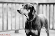
(a) Animals

(b) Textures

(c) Signs

(d) Omniglot

(e) Digits

(f) Aircraft

(g) Flowers

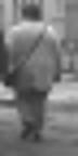
(h) Pedestrian

Figure 1: Image examples from different domains.

In this paper, we propose a multi-domain learning approach based on depthwise separable convolution. Depthwise separable convolution has been proved to be a powerful variation of standard convolution for many applications, such as image classification (?), natural language processing (?) and embedded vision applications (?). To the best of our knowledge, this is the first work that explores depthwise separable convolution for multi-domain learning. The proposed multi-domain learning model is compact and easily extensible. To promote knowledge transfer between different domains we further introduce a softmax gating mechanism. We evaluate our method on Visual Decathlon Challenge (?), a benchmark for testing multi-domain learning models. Our method can beat the state-of-the-art models with only 50% of the parameters.

Summary and contributions: The contributions of this paper are summarized below:

• We propose a novel multi-domain learning approach by exploiting the structure regularity hidden in different domains. The proposed approach greatly reduces the number of parameters and can be easily adapted to work on new domains.

• The proposed approach is based on the assumption that images in different domains share cross-channel correlations while having domain-specific spatial correlations. We validate the assumption by analyzing the visual concepts captured by depthwise separable convolution using network dissection (?).

• Our approach outperforms the state-of-the-art results on Visual Decathlon Challenge with only 50% of the parameters.

Related Work

Multi-Domain Learning Multi-domain learning aims at creating a single neural network to perform image classification tasks in a variety of domains. (?) showed that a single neural network can learn simultaneously several different visual domains by using an instance normalization layer. (?; ?) proposed universal parametric families of neural networks that contain specialized problem-specific models which differ only by a small number of parameters. (?) proposed a method called Deep Adaptation Networks (DAN) that constrains newly learned filters for new domains to be linear combinations of existing ones. Multi-domain learning can promote the application of deep learning based vision models since it reduces engineers’ effort to train new models for new images.

Multi-Task Learning The goal of multi-task learning (?; ?; ?; ?) is to extract different features from a single input to simultaneously perform classification, object recognition, edge detection, etc. Various applications can be benefited from a multi-task learning approach since the training signals can be reused among related tasks (?; ?).

Transfer Learning The goal of transfer learning is to improve the performance of a model on a target domain by leveraging the information from a related source domain (?; ?; ?). Transfer learning has wide applications in a variety of areas, such as computer vision (?), sentiment analysis (?) and recommender systems (?; ?). Different from transfer learning, multi-domain learning aims at maximizing the performance of the model across multiple domains rather than focusing on a specific target domain.

Preliminary

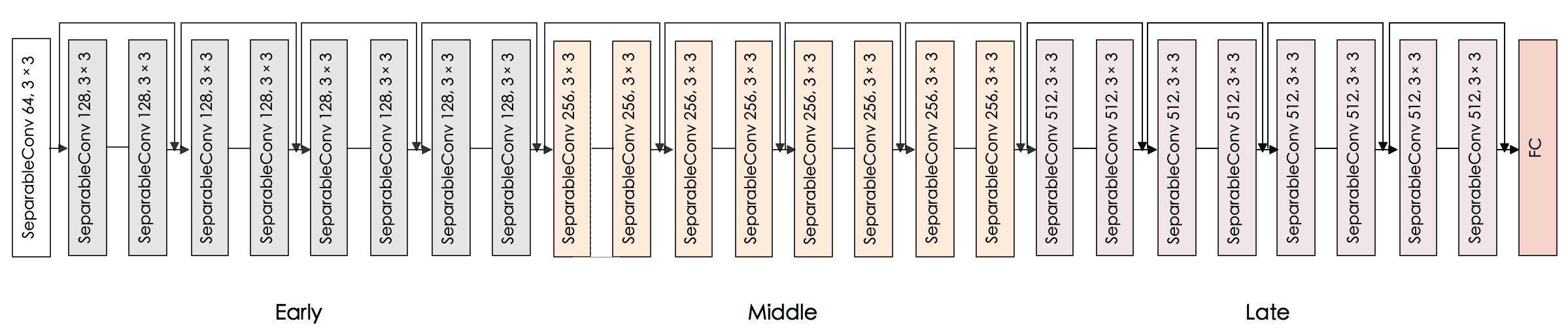
Figure 2: ResNet-26 with depthwise separable convolution.

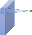
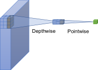
Figure 3: Standard convolution and depthwise separable convolution.

Problem Definition and Notations

Consider a set of image domains $\{D_{1},D_{2},...,D_{T}\}$, each domain $D_{i}$ consists of a triplet $\{X_{i},Y_{i},P_{i}\}$. $X_{i}\in\mathbb{R}^{C_{i}\times H_{i}\times W_{i}}$ is the input image space and $Y_{i}\in\{1,2,...,L_{i}\}$ is the output label space. Let $x\in X_{i}$ and $y\in Y_{i}$ be a pair of objects. The joint probabilistic distribution $P_{i}(x,y)$ describes the frequency of encountering $(x,y)$ in domain $D_{i}$. For a neural network $g_{i}(x)$: $\mathbb{R}^{C_{i}\times H_{i}\times W_{i}}\rightarrow\{1,2,...,L_{i}\}$ and a given loss function $l$, the risk of $g_{i}(x)$ can be measured as below,

$$R_{i}=\mathbb{E}[l(y,g_{i}(x)]=\int l(y,g_{i}(x))dP_{i}(x,y)$$ (1)

In multi-domain learning, our goal is to design neural network architectures that can work well on all the domains simultaneously. Let $\mathcal{E}_{(D_{i})}$ be the domain-specific parameters for domain $D_{i}$ and $\mathcal{C}$ be the sharable portion of the neural network. For $x\in X_{i}$, the output of the network can be calculated as,

$$\hat{y}=(\mathcal{E}_{(D_{i})}\circ\mathcal{C})(x)$$ (2)

The average risk of the neural network across all the domains can be expressed as,

$$R=\frac{1}{T}\sum_{i=1}^{T}\mathbb{E}[l(y,(\mathcal{E}_{(D_{i})}\circ\mathcal{C})(x)]$$ (3)

The goals of multi-domain learning include: (1) minimize the average risk across different domains; (2) maximize the size of sharing part $\mathcal{C}$; (3) minimize the size of the domain-specific part $\mathcal{E}_{(D_{i})}$.

Depthwise Separable Convolution

Our proposed approach is based on depthwise separable convolution that factorizes a standard $3\times 3$ convolution into a $3\times 3$ depthwise convolution and a $1\times 1$ pointwise convolution. While standard convolution performs the channel-wise and spatial-wise computation in one step, depthwise separable convolution splits the computation into two steps: depthwise convolution applies a single convolutional filter per each input channel and pointwise convolution is used to create a linear combination of the output of the depthwise convolution. The comparison of standard convolution and depthwise separable convolution is shown in Fig. 3.

Consider applying a standard convolutional filter $K$ of size $W\times W\times M\times N$ on an input feature map $F$ of size $D_{f}\times D_{f}\times M$ and produces an output feature map $O$ is of size $D_{f}\times D_{f}\times N$,

$$O_{k,l,n}=\sum_{i,j,m}K_{i,j,m,n}\cdot F_{k+i-1,l+j-1,m}$$ (4)

In depthwise separable convolution, we factorize above computation into two steps. The first step applies a $3\times 3$ depthwise convolution $\hat{K}$ to each input channel,

$$\hat{O}_{k,l,m}=\sum_{i,j}\hat{K}_{i,j,m}\cdot F_{k+i-1,l+j-1,m}$$ (5)

The second step applies $1\times 1$ pointwise convolution $\tilde{K}$ to combine the output of depthwise convolution,

$$O_{k,l,n}=\sum_{m}\tilde{K}_{m,n}\cdot\hat{O}_{k-1,l-1,m}$$ (6)

Depthwise convolution and pointwise convolution have different roles in generating new features: the former is used for capturing spatial correlations while the latter is used for capturing channel-wise correlations.

Most the previous works (?; ?; ?) focus on the computational aspect of depthwise separable convolution since it requires less parameters than standard convolution and is more computationally effective. In (?), the authors proposed the “Inception hypothesis” stating that mapping cross-channel correlations and spatial correlations separately is more efficient than mapping them at once. In this paper, we provide further evidence to support this hypothesis in the setting of multi-domain learning. We validate the assumption that images from different domains share cross-channel correlations but have domain-specific spatial correlations. Based on this idea, we develop a highly efficient multi-domain learning method. We further analyze the visual concepts captured by depthwise convolution and pointwise convolution based on network dissection (?). The visualization results show that while having less parameters depthwise convolution captures more concepts than pointwise convolution.

Proposed Approach

Network Architecture

For the experiments, we use the same ResNet-26 architecture as in (?). This allows us to fairly compare the performance of the proposed approach with previous ones. This original architecture has three macro residual blocks, each outputting 64, 128, 256 feature channels. Each macro block consists of 4 residual blocks. Each residual block has two convolutional layers consisting of 3 $\times$ 3 convolutional filters. The network ends with a global average pooling layer and a softmax layer for classification.

Different from (?), we replace each standard convolution in the ResNet-26 with depthwise separable convolution and increase the channel size. The modified network architecture is shown in Fig. 2. This choice leads to a more compact model while still maintaining enough network capacity. The original ResNet-26 has over 6M parameters while our modified architecture has only half the amount of parameters. In the experiments we found that the reduction of parameters does no harm to the performance of the model. The use of depthwise separable convolution allows us to model cross-channel correlations and spatial correlations separately. The idea behind our multi-domain learning method is to leverage the different roles of cross-channel correlations and spatial correlations in generating image features by sharing the pointwise convolution across different domains.

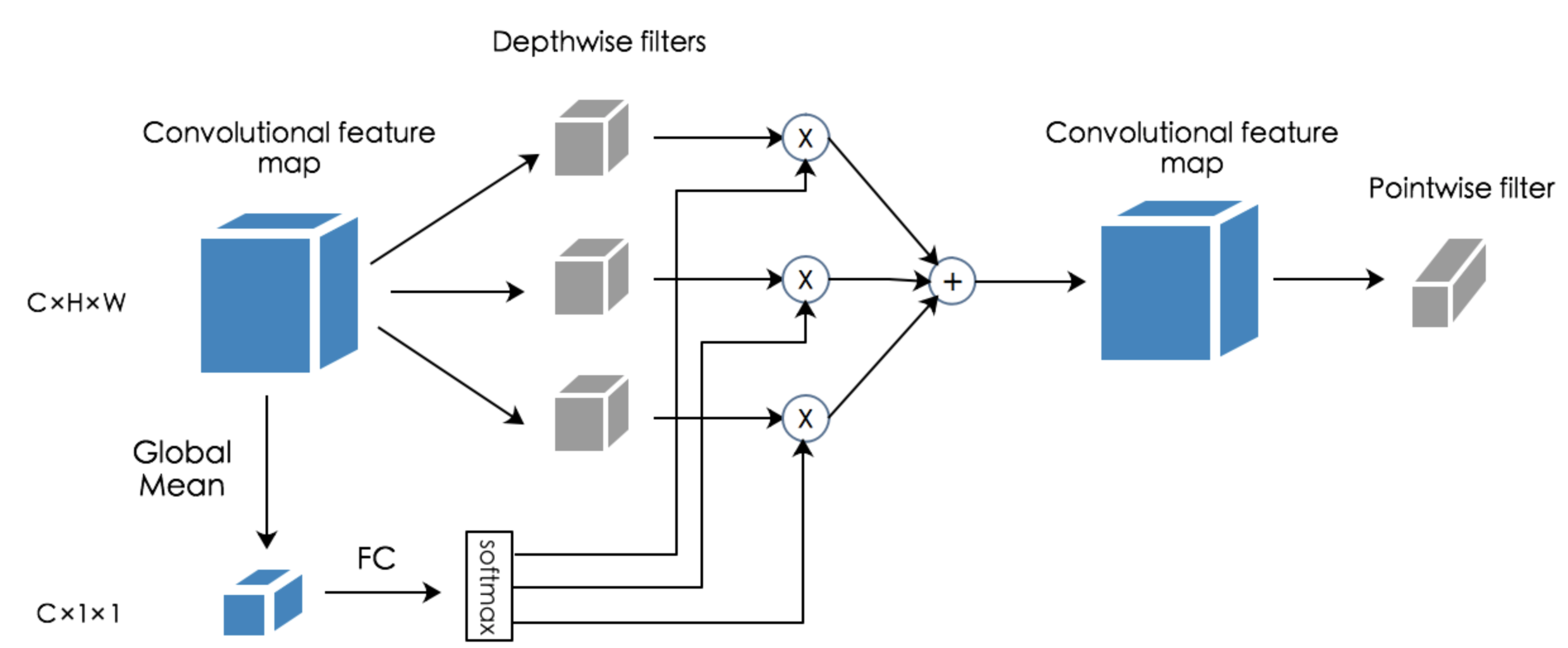
Figure 4: The proposed soft-sharing approach for sharing spatial correlations.

Learning Multiple Domains

For multi-domain learning, it is essential to have a set of universally sharable parameters that can generalize to unseen domains. To get a good starting set of parameters, we first train the modified ResNet-26 on ImageNet. After we obtain a well-initialized network, each time when a new domain arrives, we add a new output layer and finetune the depth-wise convolutional filters. The pointwise convolutional filters are shared accross different domains. Since the statistics of the images from different domains are different, we also allow domain-specific batch normalization parameters. During inference, we stack the trained depthwise convolutional filters for all domains as a 4D tensor and the output of domain $d$ can be calculated as,

$$\hat{O}_{k,l,m,d}=\sum_{i,j}\hat{K}_{i,j,m,d}\cdot F_{k+i-1,l+j-1,m,d}$$ (7)

The adoption of depthwise separable convolution provides a natural separation for modeling cross-channel correlations and spatial correlations. Experimental evidence (?) suggests the decouple of cross-channel correlations and spatial correlations would result in more useful features. We take one step further to develop a multi-domain domain method based on the assumption that different domains share cross-channel correlations but have domain-specific spatial correlations. Our method is based on two observations: model efficiency and interpretability of hidden units in a deep neural network.

Model efficiency Table 1 shows the comparison of standard $3\times 3$ convolution, $3\times 3$ depthwise convolution (Dwise) and $1\times 1$ pointwise convolution (Pwise). Clearly, standard convolution has far more parameters than both depthwise convolution ($\times c_{2}$) and pointwise convolution ($\times 9$). Typically, pointwise convolution has more parameters than depthwise convolution. In the architecture shown in Fig 2, pointwise convolution accounts for 80% of the parameters in the convolutional layers. The choice of sharing pointwise convolution and adding depthwise convolution induces minimal additional parameters when dealing with new domains. In the experiments we found that only by adding depthwise convolution leads to a network with limited number of free parameters which cannot handle some large datasets. To increase the network capacity, we allow the last convolutional layer to be specific for each domain. Based on this modification, each new domain averagely introduces 0.3M additional parameters which is 10% of the modified ResNet-26.

Interpretability While depthwise convolution typical has less paramaters, by using the technique of network dissection (?), we found it captures more visual concepts than pointwise convolution. Meanwhile, the results in the same convolutional layer show that depthwise convolution captures higher level concepts such as wheel and grass while pointwise convolution can only detect dots or honeycombed. This observation suggests that pointwise convolution can be generally shared between different image domains since it is typically used for dealing with lower level features.

Input	Operator	Output	Parameters
$c_{1}\times h\times w$	$3\times 3\textnormal{ Conv2d}$	$c_{2}\times h\times w$	$3\times 3\times c_{1}\times c_{2}$
$c_{1}\times h\times w$	$3\times 3\textnormal{ Dwise }$	$c_{1}\times h\times w$	$3\times 3\times c_{1}$
$c_{1}\times h\times w$	$1\times 1\textnormal{ Pwise }$	$c_{2}\times h\times w$	$1\times 1\times c_{1}\times c_{2}$

Table 1: Comparison of standard $3\times 3$ convolution, $3\times 3$ depthwise convolution (Dwise) and $1\times 1$ pointwise convolution (Pwise).

Soft Sharing of Trained Depthwise Filters

In addition to the proposed sharing pointwise filters (cross-channel correlations) for multi-domain learning, we also investigate whether the depthwise filters (spatial correlations) learned from other domains can be transferred to the target domain. We introduce a novel soft sharing approach in the multi-domain setting to allow the sharing of depthwise convolution. We first train domain-specific depthwise filters. Then we stack all the domain-specific filters as in Fig 4. During soft-sharing, we train each domain one by one. All the domain-specific depthwise filters and pointwise filters (trained on ImageNet) are fixed during soft sharing. We only train the feedforward network that controls the softmax gate. For a specific target domain, the softmax gate allows a soft sharing of trained depthwise filters with other domains. It can be denoted as follows: for each domain $D_{j}$, consider a network with $L$ depthwise separable convolutional layers $S_{1},...,S_{L}$, the input to the pointwise convolution in layer $l$ is defined as,

$$\hat{O}^{l}=\sum_{i=1}^{T}s^{l}_{i}\hat{O}^{l}_{i},\quad\textnormal{with}\sum_{i=1}^{T}s^{l}_{i}=1$$ (8)

where $\hat{O}^{l}_{i}$ is the output of the depthwise convolution of domain $i$ in the layer $l$ if we use images in domain $D_{j}$ as input. $s^{l}_{i}$ denotes a learned scale for the depthwise convolution of domain $i$ in the layer $l$. The scales $s_{1},...,s_{T}$ are the output of a softmax gate. The input to the softmax gate is the convolutional feature map $X_{l-1}\in\mathbb{R}^{C\times H\times W}$ produced by the previous layer. Similar to (?), we only consider global channel-wise features. In particular, we perform global average pooling to compute channel-wise means,

$$M_{c}=\frac{1}{H\times W}\sum_{i=1}^{H}\sum_{j=1}^{W}X_{c,i,j}$$ (9)

The output is a 3-dimensional tensor of size $C\times 1\times 1$. To achieve a lightweight design, we adopt a simple feedforward network consisting of two linear layers with ReLU activations to apply a nonlinear transformation on the channel-wise means and feed the output to the softmax gate. All the convolutional filters are freezed during soft sharing. The scales $s_{1},...,s_{T}$ and the parameters of the feedforward networks are learnt jointly via backpropagation.

It is widely believed that early layers in a convolutional neural network are used for detecting lower level features such as textures while later layers are used for detecting parts or objects. Based on this observation, we partition the network into three regions (early, middle, late) as shown in Figure 2 and consider different placement of the softmax gate which allows us to compare a variety of sharing strategies.

Experiment

Datasets and evaluation metrics

We evaluate our approach on Visual Domain Decathlon Challenge (?). It is a challenge to test the ability of visual recognition algorithms to cope with images from different visual domains. There are a total of 10 datasets: (1) ImageNet (2) CIFAR-100 (3) Aircraft (4) Daimler pedestrian classification (5) Describable textures (6) German traffic signs (7) Omniglot (8) SVHN (9) UCF101 Dynamic Images (10) VGG-Flowers. The detailed statistics of the datasets can be found at http://www.robots.ox.ac.uk/~vgg/decathlon/.

The performance is measured in terms of a single scalar score $S=\sum_{i=1}^{10}\alpha_{i}\textnormal{max}\{0,E_{i}^{\textnormal{max}}-E_{i}\}^{\gamma_{i}}$,where $E_{i}=\frac{1}{D_{i}^{\textnormal{test}}}\sum_{(x,y)\in D_{i}^{\textnormal{test}}}1\{y\neq(\mathcal{E}_{(D_{i})}\circ\mathcal{C})(x)\}$. $E_{i}$ is the average test error of domain $D_{i}$. $E_{i}^{\textnormal{max}}$ is the error of a reasonable baseline algorithm. The exponent $\gamma_{i}$ is set to be 2 for all domains. The coefficient $\alpha_{i}$ is $1000(E_{i}^{\textnormal{max}})^{-\gamma_{i}}$ then a perfect classifier receives 1000. The maximum score achieved across 10 domains is 10000.

Baselines

We consider the following baselines in the experiments,

1. Individual Network: The simplest baseline we consider is Individual Network. We finetune the pretrained modified ResNet-26 on each domain which leads to 10 models altogether. This approach results in the largest model size since there is no sharing between different domains.

2. Classifier Only: We freeze the feature extractor part of the pretrained modified ResNet-26 on ImageNet and train domain-specific classifier layer for each domain.

3. Depthwise Sharing: Rather than sharing pointwise convolution, we consider an alternative approach of multi-domain extension of depthwise separable convolution which shares the depthwise convolution between different domains.

4. Residual Adapters: Residual Adapters (?; ?) are the state-of-the-art approaches for multi-domain learning which include Serial Residual Adapter (?) and Parallel Residual Adapter (?).

5. Deep Adaptation Networks (DAN): In (?) the authors propose Deep Adaptation Networks (DAN) that constrains newly learned filters for new domains to be linear combinations of existing ones via controller modules.

6. PiggyBack: In (?) the authors present PiggyBack for adding multiple tasks to a single network by learning domain-specific binary masks. The main idea is derived from network quantization (?; ?) and pruning.

Model	#par	ImNet	Airc.	C100	DPed	DTD	GTSR	Flwr	OGlt	SVHN	UCF	mean	S
# images		1.3m	7k	50k	30k	4k	40k	2k	26k	70k	9k
Serial Res. Adapt.	$2\times$	59.67	61.87	81.20	93.88	57.13	97.57	81.67	89.62	96.13	50.12	76.89	2621
Parallel Res. Adapt.	$2\times$	60.32	64.21	81.91	94.73	58.83	99.38	84.68	89.21	96.54	50.94	78.07	3412
DAN	$2.17\times$	57.74	64.12	80.07	91.30	56.64	98.46	86.05	89.67	96.77	49.38	77.01	2851
Piggyback	$1.28\times$	57.69	65.29	79.87	96.99	57.45	97.27	79.09	87.63	97.24	47.48	76.60	2838
Individual Network	$5\times$	63.99	65.71	78.26	88.29	52.19	98.76	83.17	90.04	96.84	48.35	76.56	2756
Classifier Only	$0.6\times$	63.99	51.04	75.32	94.49	54.21	98.48	84.47	86.66	95.14	43.75	74.76	2446
Depthwise Sharing	$4\times$	63.99	67.42	74.46	95.60	54.85	98.52	87.34	89.88	96.62	50.39	77.91	3234
Proposed Approach	$1\times$	63.99	61.06	81.20	97.00	55.48	99.27	85.67	89.12	96.16	49.33	77.82	3507

Table 2: Top-1 classification accuracy and the Visual Decathlon Challenge score (S) of the proposed approach and baselines. #par is the number of parameters w.r.t. the proposed approach.

Model	ImNet	Airc.	C100	DPed	DTD	GTSR	Flwr	OGlt	SVHN	UCF	mean	S
# images	1.3m	7k	50k	30k	4k	40k	2k	26k	70k	9k
early	63.99	58.69	81.01	95.44	55.75	98.75	84.90	88.80	96.18	48.86	77.23	3102
middle	63.99	59.11	80.93	95.33	54.74	98.71	85.42	88.93	96.09	48.91	77.21	3086
late	63.99	58.81	80.93	96.63	54.74	98.91	84.79	89.35	96.30	49.01	77.88	3303

Table 3: Top-1 classification accuracy and the Visual Decathlon Challenge score (S) of different soft sharing strategies.

Implementation details

All networks were implemented using Pytorch and trained on 2 NVIDIA V100 GPUs. For the base network trained on ImageNet we use SGD with momentum as the optimizer. We set the momentum rate to be 0.9, the initial learning rate to be 0.1 and use a batch size of 256. We train the network with a total of 120 epochs and the learning rate decays twice at 80th and 100th epoch with a factor of 10. To prevent overfitting, we use a weight decay (L2 regularization) rate of 0.0001.

For the multi-domain extension of depthwise separable convolution, we keep the same optimization settings as training the base network. We train the network with a total of 100 epochs and the learning rate decays twice at 60th and 80th epoch by a factor of 10. We apply weight decay (L2 regularization) to prevent overfitting. Since the size of the datasets are highly unbalanced, we use different weight decay parameters for different domains. Similar to (?), higher weight decay parameters are used for smaller datasets. In particular, 0.002 for DTD, 0.0005 for Aircraft, CIFAR100, Daimler pedestrain, Omniglot and UCF101, and 0.0003 for GTSTB, SVHN and VGG-Flowers.

For soft sharing, we train the network with a total of 10 epochs and the learning rate decays once at the 5th epoch with a factor of 10. Other settings are kept the same as training multi-domain models.

Results and Analysis

Quantitative Results

The results of the proposed approach and the baselines on Visual Decathlon Challenge are shown in Table 2. Our approach achieves the highest score among all the methods while requiring the least amount of parameters. In particular, the proposed approach improves the current state-of-the-art approaches by 100 points with only 50% of the parameters. The ResNet-26 with depthwise separable convolution surpasses the performance of the original ResNet-26 by a large margin on ImageNet (63.99 vs 60.32). On other smaller datasets, our approach still achieves better or comparable performance to the baselines. The improvement can be attributed to the sharing of pointwise convolution that has a regularization effect and allows the training signals in ImageNet to be reused when training new domains.

Compared with other variations of the modified ResNet-26, our approach still achieves the highest score. Our approach obtains a remarkable improvement (3507 vs 2756) with only 20% of the parameters compared with Individual Network. One reason for the improvement is that the proposed approach is more robust to overfitting, especially for some small datasets. While only training domain-specific classifier layers leads to the smallest model, the score is about 1000 points lower than the proposed approach. Compared with Depthwise Sharing, the assumption of sharing pointwise convolution leads to a more compact and efficient model (3507 vs 3234). This validates our assumption that it is preferable to share pointwise convolution rather than depthwise convolution in the setting of mutli-domain learning. We provide more qualitative results in the next section to support this claim.

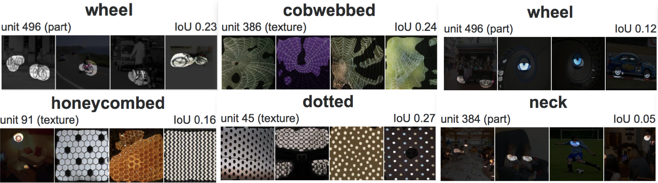
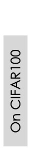
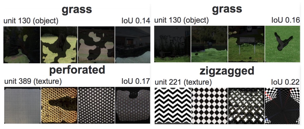
Figure 5: A comparison of visual concepts identified by network dissection in ResNet-26 with depthwise separable convolution trained on ImageNet and CIFAR100. The first two rows demonstrate the results on ImageNet and the last two rows demonstrate the results on CIFAR100. The columns show the results in different layers. The highest-IoU matches among hidden units of each layer are shown. The hidden units of the pointwise convolution in the 18th layer detect no visual concepts.

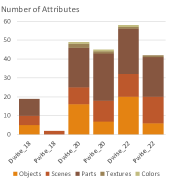
(a) On ImageNet

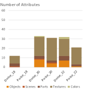
(b) On CIFAR100

Figure 6: Number of attributes captured by the hidden units of depthwise convolution and pointwise convolution in the 18th, 20th and 22th convolutional layer.

Qualitative Results

This section presents our visualization results of deptwise convolution and pointwise convolution based on network dissection (?). Network dissection is a general framework for quantifying the interpretability of deep neural networks by evaluating the alignment between individual hidden units and a set of semantic concepts. The accuracy of unit $k$ in detecting concept $c$ is denoted as $IoU_{k,c}$. If the value of $IoU_{k,c}$ exceeds a threshold then we consider the unit $k$ as a detector for the concept $c$. The details of calculating $IoU_{k,c}$ is omited due to space limitation.

In the experiments, we use the individual networks trained on ImageNet and CIFAR100 as examples. We visualize the hidden units in the 18th, 20th, 22th convolutional layers. Fig 5 shows the interpretability of units of the depthwise convolution and pointwise convolution in the corresponding layer. The highest-IoU matches among hidden units of each layer are shown. We observe that the hidden units in depthwise convolution detect higher level concepts than the units in pointwise convolution. The units in the depthwise convolution can capture part or object while the units in pointwise convolution can only detect textures. Moreover, Fig 6 shows the number of attributes captured by the units in depth convolution and pointwise convolution. The results demonstrate that depthwise convolution consistently detects more attributes than pointwise convolution. These observations imply that pointwise convolution are mostly used for capturing low level features which can be generally shared across different domains.

Soft Sharing of Trained Depthwise Filters

Table 3 shows the results of soft sharing. Regardless of the different placements of the softmax gate, the base approach without sharing still achieves the highest score on Visual Decathlon Challenge. One possible reason is that the datasets are from very different domains, sharing information between them may not generally improve the performance. However, for some specific datasets, we still observe some improvement. In particular, by sharing early layers we can obtain a slightly higher accuracy on DTD and SVHN. Another observation is that sharing later layers leads to a higher score than other alternatives. This implies that although images in different domain may not share similar low level features, they can still be benefited from each other by transfering information in later layers.

Conclusion

In this paper, we present a multi-domain learning approach based on depthwise separable convolution. The proposed approach is based on the assumption that images from different domains share the same channel-wise correlation but have domain-specific spatial-wise correlation. We evaluate our approach on Visual Decathlon Challenge and achieve the highest score among the current approaches. We further visualize the concepts detected by the hidden units in depthwise convolution and pointwise convolution. The results reveal that depthwise convolution captures more attributes and higher level concepts than pointwise convolution.

References

- [Bau et al. 2017] Bau, D.; Zhou, B.; Khosla, A.; Oliva, A.; and Torralba, A. 2017. Network dissection: Quantifying interpretability of deep visual representations. arXiv preprint arXiv:1704.05796.
- [Bengio 2012] Bengio, Y. 2012. Deep learning of representations for unsupervised and transfer learning. In Proceedings of ICML Workshop on Unsupervised and Transfer Learning, 17–36.
- [Bilen and Vedaldi 2016] Bilen, H., and Vedaldi, A. 2016. Integrated perception with recurrent multi-task neural networks. In Advances in neural information processing systems, 235–243.
- [Bilen and Vedaldi 2017] Bilen, H., and Vedaldi, A. 2017. Universal representations: The missing link between faces, text, planktons, and cat breeds. arXiv preprint arXiv:1701.07275.
- [Caruana 1997] Caruana, R. 1997. Multitask learning. Machine learning 28(1):41–75.
- [Chollet 2017] Chollet, F. 2017. Xception: Deep learning with depthwise separable convolutions. In 2017 IEEE Conference on Computer Vision and Pattern Recognition (CVPR), 1800–1807. IEEE.
- [Cichon and Gan 2015] Cichon, J., and Gan, W.-B. 2015. Branch-specific dendritic ca2+ spikes cause persistent synaptic plasticity. Nature 520(7546):180–185.
- [Courbariaux et al. 2016] Courbariaux, M.; Hubara, I.; Soudry, D.; El-Yaniv, R.; and Bengio, Y. 2016. Binarized neural networks: Training deep neural networks with weights and activations constrained to+ 1 or-1. arXiv preprint arXiv:1602.02830.
- [Doersch and Zisserman 2017] Doersch, C., and Zisserman, A. 2017. Multi-task self-supervised visual learning. In The IEEE International Conference on Computer Vision (ICCV).
- [Glorot, Bordes, and Bengio 2011] Glorot, X.; Bordes, A.; and Bengio, Y. 2011. Domain adaptation for large-scale sentiment classification: A deep learning approach. In Proceedings of the 28th international conference on machine learning (ICML-11), 513–520.
- [Guo, Wang, and Xu 2015] Guo, Y.; Wang, X.; and Xu, C. 2015. Crorank: cross domain personalized transfer ranking for collaborative filtering. In Data Mining Workshop (ICDMW), 2015 IEEE International Conference on Data Mining, 1204–1212. IEEE.
- [Guo 2018] Guo, Y. 2018. A survey on methods and theories of quantized neural networks. arXiv preprint arXiv:1808.04752.
- [Hayashi-Takagi et al. 2015] Hayashi-Takagi, A.; Yagishita, S.; Nakamura, M.; Shirai, F.; Wu, Y. I.; Loshbaugh, A. L.; Kuhlman, B.; Hahn, K. M.; and Kasai, H. 2015. Labelling and optical erasure of synaptic memory traces in the motor cortex. Nature 525(7569):333.
- [He et al. 2016] He, K.; Zhang, X.; Ren, S.; and Sun, J. 2016. Deep residual learning for image recognition. In Proceedings of the IEEE conference on computer vision and pattern recognition, 770–778.
- [Howard et al. 2017] Howard, A. G.; Zhu, M.; Chen, B.; Kalenichenko, D.; Wang, W.; Weyand, T.; Andreetto, M.; and Adam, H. 2017. Mobilenets: Efficient convolutional neural networks for mobile vision applications. arXiv preprint arXiv:1704.04861.
- [Hu, Lu, and Tan 2015] Hu, J.; Lu, J.; and Tan, Y.-P. 2015. Deep transfer metric learning. In Proceedings of the IEEE Conference on Computer Vision and Pattern Recognition, 325–333.
- [Kaiser, Gomez, and Chollet 2017] Kaiser, L.; Gomez, A. N.; and Chollet, F. 2017. Depthwise separable convolutions for neural machine translation. arXiv preprint arXiv:1706.03059.
- [Kirkpatrick et al. 2017] Kirkpatrick, J.; Pascanu, R.; Rabinowitz, N.; Veness, J.; Desjardins, G.; Rusu, A. A.; Milan, K.; Quan, J.; Ramalho, T.; Grabska-Barwinska, A.; et al. 2017. Overcoming catastrophic forgetting in neural networks. Proceedings of the national academy of sciences 201611835.
- [Kokkinos 2017] Kokkinos, I. 2017. Ubernet: Training a universal convolutional neural network for low-, mid-, and high-level vision using diverse datasets and limited memory. In 2017 IEEE Conference on Computer Vision and Pattern Recognition (CVPR), 5454–5463. IEEE.
- [Krizhevsky, Sutskever, and Hinton 2012] Krizhevsky, A.; Sutskever, I.; and Hinton, G. E. 2012. Imagenet classification with deep convolutional neural networks. In Advances in neural information processing systems, 1097–1105.
- [Li and Hoiem 2017] Li, Z., and Hoiem, D. 2017. Learning without forgetting. IEEE Transactions on Pattern Analysis and Machine Intelligence.
- [Mallya and Lazebnik 2018] Mallya, A., and Lazebnik, S. 2018. Piggyback: Adding multiple tasks to a single, fixed network by learning to mask. arXiv preprint arXiv:1801.06519.
- [Pan et al. 2010] Pan, W.; Xiang, E. W.; Liu, N. N.; and Yang, Q. 2010. Transfer learning in collaborative filtering for sparsity reduction.
- [Pan, Yang, and others 2010] Pan, S. J.; Yang, Q.; et al. 2010. A survey on transfer learning. IEEE Transactions on knowledge and data engineering 22(10):1345–1359.
- [Raina et al. 2007] Raina, R.; Battle, A.; Lee, H.; Packer, B.; and Ng, A. Y. 2007. Self-taught learning: transfer learning from unlabeled data. In Proceedings of the 24th international conference on Machine learning, 759–766. ACM.
- [Rebuffi, Bilen, and Vedaldi 2017] Rebuffi, S.-A.; Bilen, H.; and Vedaldi, A. 2017. Learning multiple visual domains with residual adapters. In Advances in Neural Information Processing Systems, 506–516.
- [Rebuffi, Bilen, and Vedaldi 2018] Rebuffi, S.-A.; Bilen, H.; and Vedaldi, A. 2018. Efficient parametrization of multi-domain deep neural networks. In IEEE Conference on Computer Vision and Pattern Recognition (CVPR).
- [Rosenfeld and Tsotsos 2017] Rosenfeld, A., and Tsotsos, J. K. 2017. Incremental learning through deep adaptation. arXiv preprint arXiv:1705.04228.
- [Sandler et al. 2018] Sandler, M.; Howard, A.; Zhu, M.; Zhmoginov, A.; and Chen, L.-C. 2018. Inverted residuals and linear bottlenecks: Mobile networks for classification, detection and segmentation. arXiv preprint arXiv:1801.04381.
- [Veit and Belongie 2017] Veit, A., and Belongie, S. 2017. Convolutional networks with adaptive computation graphs. arXiv preprint arXiv:1711.11503.
- [Wang, He, and Gupta 2017] Wang, X.; He, K.; and Gupta, A. 2017. Transitive invariance for selfsupervised visual representation learning. In Proc. of Int’l Conf. on Computer Vision (ICCV).
- [Gan et al. 2017] Gan, C.; Li, Y.; Li, H.; Sun, C.; and Gong, B. 2017. Vqs: Linking segmentations to questions and answers for supervised attention in vqa and question-focused semantic segmentation. In The IEEE International Conference on Computer Vision (ICCV).
- [Long et al. 2018] Long, X.; Gan, C.; de Melo, G.; Liu, X.; Li, Y.; Li, F.; and Wen, S. 2018. Multimodal keyless attention fusion for video classification. In Thirty-Second AAAI Conference on Artificial Intelligence.
- [Li et al. 2018] Li, Y.; Wang, L.; Yang, T.; and Gong, B. 2018. How local is the local diversity? reinforcing sequential determinantal point processes with dynamic ground sets for supervised video summarization. In The European Conference on Computer Vision (ECCV).
- [Zamir et al. 2018] Zamir, A. R.; Sax, A.; Shen, W.; Guibas, L.; Malik, J.; and Savarese, S. 2018. Taskonomy: Disentangling task transfer learning. In Proceedings of the IEEE Conference on Computer Vision and Pattern Recognition, 3712–3722.