Approximation of the first passage time distribution for the birth–death processes

Abstract

We propose a general method to obtain approximation of the first passage time distribution for the birth–death processes. We rely on the general properties of birth–death processes, Keilson’s theorem and the concept of Riemann sum to obtain closed–form expressions. We apply the method to the three selected birth–death processes and the sophisticated order–book model exhibiting long–range memory. We discuss how our approach contributes to the competition between spurious and true long–range memory models.

1 Introduction

Markov chains, and more specifically birth–death processes, are of great interest in the modeling of biological and socio–economic systems [1, 2, 3]. While usually birth–death processes converge to some fixed point, in which birth and death rates are approximately equal, there are also a few examples which do not converge and system–wide fluctuations persist [4, 5, 6]. This strand of research is important and present in various fields of science, because it could provide an answer to Axelrod’s question about the persistence of diversity in social systems [7, 8]. The question of diversity, and especially the collapses of diversity, is also important to the financial markets. Some recent financial agent–based models (abbr. ABMs) have demonstrated that power–law distributions emerge, when the diversity breaks down and agents start to behave similarly [9, 10, 11, 12, 13, 14]. One of the approaches, based on the birth–death process, [9] has explicitly shown that the long–range memory phenomenon could emerge due to the same underlying reasons.

Long–range memory phenomenon can be reproduced using non–linear Markov processes [15, 16] and models with embedded memory, such as ones built using fractional Brownian motion [17, 18, 19, 20, 21], CTRW framework [22, 23, 24, 25, 26, 27] or ARCH framework [28, 29, 30]. Though these models are able to reproduce few similar statistical features, they differ in their first passage times [17, 31, 32]. It is known that first passage time probability density function (PDF) of fractional Brownian motion have a region with power–law dependence with exponent $H-2$ [17], while first passage time PDF of one–dimensional Markov processes has power–law exponent of $-3/2$ [31, 32]. Which naturally suggests a method to determine whether the observed long–range memory phenomenon is spurious or not.

The problem arises, because the current knowledge describes the asymptotic behavior of the first passage time PDFs in very broad terms. There is an alternative description using Laplace transforms, yet these are often expressed using infinite sums and special functions [33]. With a few notable exceptions, usually such Laplace transforms are not invertible and even if they are invertible they might not have explicit closed–forms. Consequently there has been numerical efforts to approximate the inverses [34].

Here we propose a general method to analytically approximate specific first passage times of birth–death processes. We build upon our previous work [35] in which we have obtained an approximation for a specific first passage time, called inter–burst duration, PDF of the continuous Bessel process. We have shown that the approximation could be applied to a diffusion process transformable into Bessel process (with stochastic process described in [36] provided as an example). Notably the approximation had a divergence problem for short times, which we now solve by proposing to study birth–death processes with finite and discrete state space.

The paper is organized as follows. In Section 2 we introduce the concept of the bursting statistics in the context of the continuous Bessel process. In Section 3 we introduce approximation method based on Keilson’s theorem [37] and the results reported in [35]. In Section 4 we approximate bursting statistics of a few selected birth–death processes: Bessel–like, Ornstein–Uhlenbeck and imitation processes. In Section 5 we demonstrate that this approach can be used to fit the bursting statistics of a sophisticated model. Concluding remarks are provided in Section 6.

2 Bursting statistics of the continuous Bessel process

In [35, 38, 39, 40] we have considered burst durations and inter–burst durations of empirical time series and time series generated by stochastic processes. We have defined burst duration $\tau_{h}$ as a time spent above the certain threshold $h$:

$$\tau_{h}=\mathrm{Inf}\left\{t>0:F\left(t\right)\leq h|F\left(0\right)=h+\epsilon\right\},$$ (1)

here $F\left(t\right)$ describes time evolution of a stochastic process or an empirical time series, while $\epsilon$ is an infinitesimally small positive number. In a similar fashion we have defined inter–burst duration $\theta_{h}$ as a time spent below the threshold:

$$\theta_{h}=\mathrm{Inf}\left\{t>0:F\left(t\right)\geq h|F\left(0\right)=h-\epsilon\right\}.$$ (2)

In Fig. 1 we have illustrated these concepts on a sample time series. This sample contains a single example of a burst duration and a single example of an inter–burst duration.

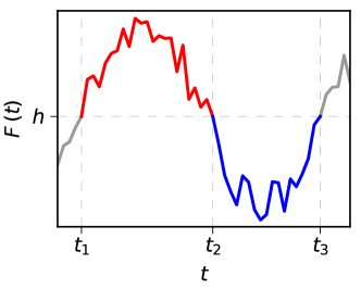
Figure 1: (color online) Sample time series (gray curve) with one time period fully spent above the threshold (highlighted in red) and one time period fully spent below the threshold (highlighted in blue). Duration $t_{2}-t_{1}$ is by definition a sample of burst duration $\tau_{h}$, while duration $t_{3}-t_{2}$ is by definition a sample of inter–burst duration $\theta_{h}$.

In [35] we have obtained an approximation for the PDF of $\theta_{h}$ for the continuous Bessel process. This was possible, because first passage times from $y_{0}$ to $h$ (with $0<y_{0}<h$) for the continuous Bessel process are known [33]:

$$p_{y_{0},h}^{\left(\nu\right)}\left(\theta_{h}\right)=\frac{h^{\nu-2}}{y_{0}^{\nu}}\sum_{k=1}^{\infty}\frac{j_{\nu,k}J_{\nu}\left(\frac{y_{0}}{h}j_{\nu,k}\right)}{J_{\nu+1}\left(j_{\nu,k}\right)}\exp\left(-\frac{j_{\nu,k}^{2}}{2h^{2}}\theta_{h}\right),$$ (3)

here $\nu$ is the index of the continuous Bessel process, $J_{\nu}\left(x\right)$ is a Bessel function of a first kind and $j_{\nu,k}$ is $k$-th zero of $J_{\nu}\left(x\right)$.

Let $y_{0}=h-\epsilon$, where $\epsilon$ is an infinitesimally small positive number, then Eq. (3) can be approximated by an integral:

$$p\left(\theta_{h}\right) \approx C_{1}\sum_{k=1}^{\infty}j_{\nu,k}^{2}\exp\left(-\frac{j_{\nu,k}^{2}}{2h_{y}^{2}}\theta_{h}\right)\approx C_{2}\int_{j_{\nu,1}}^{\infty}x^{2}\exp\left(-\frac{x^{2}}{2h_{y}^{2}}\theta_{h}\right)\mathrm{d}x=$$

$$=C_{2}\left[\frac{h_{y}^{2}j_{\nu,1}\exp\left(-\frac{j_{\nu,1}^{2}}{2h_{y}^{2}}\theta_{h}\right)}{\theta_{h}}+\sqrt{\frac{\pi}{2}}\frac{h_{y}^{3}\mathrm{erfc}\left(\frac{j_{\nu,1}}{\sqrt{2}h_{y}}\sqrt{\theta_{h}}\right)}{\theta_{h}^{3/2}}\right].$$ (4)

This approximation is possible only because $j_{\nu,k}$ grow almost linearly with $k$. For various $\nu$ only the first few values deviate from this tendency. In this case we can treat the sum as if it was a Riemann sum and replace the sum by integral. As we can see in Fig. 2 this approximation works rather well for the continuous Bessel process.

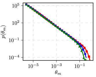
Figure 2: (color online) Inter–burst duration PDF of the continuous Bessel process with three distinct indices, $\nu=0.5$ (red squares), $1.5$ (blue circles) and $2.5$ (green triangles), at level $h=0.7$. Numerical results are approximated by Eq. (4) (respectively colored curves).

The normalization of this approximation diverges unless some minimum value of $\theta_{h}$ is assumed. To keep the expression general we have left the normalization constants denoted by $C_{i}$. While the minimum value of $\theta_{h}$ can be easily justified from empirical point of view, assuming equivalence to the discretization period, such assumption isn’t as transparent in case of a continuous model.

Note that the asymptotic behavior of Eq. (4) is consistent with what would be expected of a one–dimensional Markov processes [31]. For the small $\theta_{h}$the second term is the largest and therefore power lay decay is observed with exponent $-3/2$. For the larger $\theta_{h}$ the first term becomes the largest and the exponential cutoff is observed.

It is not possible to obtain approximation for $\tau_{m}$ of the continuous Bessel process, because for the most $\nu$ the Bessel process escapes towards infinity and therefore does not always hit $h$. Consequently there is no general formula for the hitting times of the Bessel process for $0<h<y_{0}$ case [33].

It is important to note that Eq. (4) applies to any process, which can be transformed into Bessel process by means of Lamperti transformation. Though if the Lamperti transformation stipulates inverse relationship between processes, then Eq. (4) would approximate burst duration PDF of that process instead. In [35] we have considered one such case. We have transformed a non–linear stochastic process exhibiting long–range memory [41] into Bessel process by means of Lamperti transformation. We have shown that Eq. (4) provides a good fit for the burst duration PDF of numerical simulations of the non–linear stochastic process exhibiting spurious long–range memory.

3 Approximation of inter–burst duration for any birth–death process

Through Keilson’s theorem [37, 42] it is well known that Laplace transform of a first passage time from state $k$ to state $n$, with $0<k<n$, is given by:

$$\left\langle e^{-sT_{k,n}}\right\rangle=\frac{\prod{}_{i=1}^{n}\frac{\lambda_{i}^{\left(n\right)}}{s+\lambda_{i}^{\left(n\right)}}}{\prod{}_{i=1}^{k}\frac{\lambda_{i}^{\left(k\right)}}{s+\lambda_{i}^{\left(k\right)}}},\quad s\geq 0.$$ (5)

In the above $\lambda_{i}^{\left(n\right)}$ are the sorted positive eigenvalues of negative birth–death process generator matrix truncated at rank $n$. Inverse Laplace transforms of this expression is not feasible for many reasonable values of $n$ and $k$. Yet we have observed that for some small $n$ and $k=n-1$ inverse Laplace transform yields a sum of exponents whose rates are given by $\lambda_{i}^{\left(n\right)}$. As this sum has a similar form to the one in Eq. (4) we propose to apply the same approximation method:

$$p\left(\theta_{h}\right) \approx\frac{1}{\sqrt{\lambda_{n}^{\left(n\right)}}-\sqrt{\lambda_{1}^{\left(n\right)}}}\int{}_{\sqrt{\lambda_{1}^{\left(n\right)}}}^{\sqrt{\lambda_{n}^{\left(n\right)}}}x^{2}\exp\left(-x^{2}\theta_{h}\right)\mathrm{d}x=$$

$$=\frac{1}{4\left(\sqrt{\lambda_{n}^{\left(n\right)}}-\sqrt{\lambda_{1}^{\left(n\right)}}\right)}\left[2\frac{\sqrt{\lambda_{1}^{\left(n\right)}}\exp\left(-\lambda_{1}^{\left(n\right)}\theta_{h}\right)-\sqrt{\lambda_{n}^{\left(n\right)}}\exp\left(-\lambda_{n}^{\left(n\right)}\theta_{h}\right)}{\theta_{h}}+\right.$$ (6)

$$\left.+\sqrt{\pi}\frac{\mathrm{erfc}\left(\sqrt{\lambda_{1}^{\left(n\right)}\theta_{h}}\right)-\mathrm{erfc}\left(\sqrt{\lambda_{n}^{\left(n\right)}\theta_{h}}\right)}{\theta_{h}^{3/2}}\right]=I\left(\theta_{h},\lambda_{1}^{\left(n\right)},\lambda_{n}^{\left(n\right)}\right),$$

here $\lambda_{1}^{\left(n\right)}$ is the first (smallest) positive eigenvalue, $\lambda_{n}^{\left(n\right)}$ is the last (largest) positive eigenvalue and we introduce $I\left(\theta_{h},\lambda_{1}^{\left(n\right)},\lambda_{n}^{\left(n\right)}\right)$ to simplify further notation. Similar truncation idea was used in [43] to approximate asymptotic behavior of diffusion processes. This approximation will be valid as long as $\sqrt{\lambda_{i}^{\left(n\right)}}$ grows linearly in wide range of $i$. It is worth to note that this also seems to be the only way to obtain $p\left(\theta_{h}\right)\propto\theta_{h}^{-3/2}$, which is a general result for any one–dimensional Markov process. Therefore it seems that every birth–death process should have a reasonably wide region in which $\sqrt{\lambda_{i}^{\left(n\right)}}$ grow linearly.

Note that the first order approximation, Eq. (6), is usually insufficient to approximate the PDF of $\theta_{h}$, because usually the impact of $\lambda_{1}$ term becomes undervalued. To improve the overall approximation we propose to use integral approximation from the second term in the sum onwards and to account for the first term separately. Then the second order approximation of the inter–burst duration PDF would have the following form:

$$p\left(\theta_{h}\right)\approx\rho\lambda_{1}^{\left(n\right)}\exp\left[-\lambda_{1}^{\left(n\right)}\theta_{h}\right]+\left(1-\rho\right)I\left(\theta_{h},\lambda_{2}^{\left(n\right)},\lambda_{n}^{\left(n\right)}\right).$$ (7)

Here $\rho$ is used to estimate the relative impact of the first eigenvalue term. It is evaluated by comparing the contributions to the resulting first moments, $\bar{\theta}_{t}$, of the first exponent (first term) and of the PDF approximated by the integral (second term). Then the exact first moment of the respective hitting time of a birth–death process ($\bar{\theta}_{h}$ on the right hand side of the equation):

$$\bar{\theta}_{h}=\rho\cdot\frac{1}{\lambda_{1}^{\left(n\right)}}+\left(1-\rho\right)\cdot\frac{1}{\sqrt{\lambda_{2}^{\left(n\right)}\lambda_{n}^{\left(n\right)}}}\quad\Rightarrow\quad\rho=\frac{\lambda_{1}\left(1-\sqrt{\lambda_{2}^{\left(n\right)}\lambda_{n}^{\left(n\right)}}\bar{\theta}_{h}\right)}{\lambda_{1}-\sqrt{\lambda_{2}^{\left(n\right)}\lambda_{n}^{\left(n\right)}}}.$$ (8)

Note that $\bar{\theta}_{h}$ as well as the other moments of hitting times for any birth–death process is known explicitly and can be obtained exactly (see [44] for more details). Thus if there is a need to further improve the approximation, then one could split more terms from the sum and estimate their relative impact based on the higher moments. Here we limit ourselves just to the first moment as this proves sufficient in the examples we have selected.

4 Bursting statistics of the selected birth–death processes

In this section we will explore bursting statistics of a few selected birth–death processes. We will consider Bessel–like, Ornstein–Uhlenbeck and imitation processes. Using these three examples we will show that the proposed approximation method works rather well.

While these three examples are rather different, they share one property – their states are equivalent in statistical sense:

$$X\overset{s.s.}{\equiv}N-X.$$ (9)

This property means that the burst duration and the inter–burst duration are also equivalent in statistical sense:

$$\theta_{h}\overset{s.s.}{\equiv}\tau_{1-h}.$$ (10)

Thus knowing the PDF of $\theta_{h}$ also gives us a PDF for $\tau_{1-h}$.

4.1 The birth–death Bessel–like process

Let us define the transition rates for the birth–death Bessel–like process:

$$\lambda_{b}^{+}=\frac{N^{2}}{2}\left(1+\frac{\nu_{1}+\frac{1}{2}}{X}-\frac{\nu_{2}+\frac{1}{2}}{N-X}\right),\quad\lambda_{b}^{-}=\frac{N^{2}}{2}\left(1-\frac{\nu_{1}+\frac{1}{2}}{X}+\frac{\nu_{2}+\frac{1}{2}}{N-X}\right),$$ (11)

here $N$ is the number of the available states, $X$ is the current state, $\nu_{1}$ and $\nu_{2}$ are the indices of the process. To keep these rates well behaved let us require that $\nu_{i}=\frac{1}{2}+n$ with $n\in\mathbb{N}_{0}$. With $\nu_{1}>-\frac{1}{2}$ and $\nu_{2}>-\frac{1}{2}$, in the continuous limit $N\rightarrow\infty$ (defining $x=X/N$), we get a stochastic process trapped between $x=0$ and $x=1$:

$$\mathrm{d}x=\left(\nu+\frac{1}{2}\right)\frac{2x-1}{x(1-x)}\mathrm{d}t+\mathrm{d}W.$$ (12)

Two special cases with unequal indices deserve out attention. In the continuous limit with $\nu_{1}=\nu$ and $\nu_{2}=-\frac{1}{2}$ we recover SDE of the continuous Bessel process:

$$\mathrm{d}x=\left(\nu+\frac{1}{2}\right)\frac{\mathrm{d}t}{x}+\mathrm{d}W.$$ (13)

Similar birth–death process was proposed in [45] and shown to asymptotically approach the continuous Bessel process. While with $\nu_{1}=-\frac{1}{2}$ and $\nu_{2}=\nu$ we get a stochastic process, whose potential is a shifted reflection of the Bessel process potential. In this case the potential is defined for $x\in\left(-\infty;1\right)$ instead of $\left(0;+\infty\right)$ as for the Bessel process. The corresponding SDE is given by:

$$\mathrm{d}x=-\left(\nu+\frac{1}{2}\right)\frac{\mathrm{d}t}{1-x}+\mathrm{d}W.$$ (14)

Here, seeking to retain equivalence properties Eqs. (9) and (10), we will consider only the symmetric version of this birth–death process assuming that $\nu_{1}=\nu_{2}=\nu$.

In Fig. 3 we show that burst and inter–burst durations in the symmetric version of this model are indeed equivalent in statistical sense, as blue squares and red circles trace the same shape. Furthermore the approximation by Eq. (7) provides rather good approximation for that shape. Also in Fig. 3 (d) we show that the square root of the eigenvalue spectrum indeed grows linearly in a certain region.

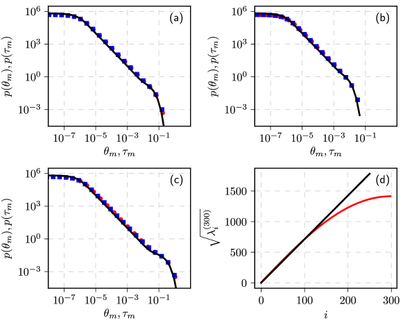
Figure 3: (color online) Burst and inter–burst duration PDFs ((a), (b) and (c)) for the symmetric case of birth–death Bessel–like process and square root of its eigenvalue spectrum (sub–figure (d)). In (a), (b) and (c) red circles represent numerical inter–burst duration PDF, blue squares represent numerical burst duration PDF, while black curve was obtained by evaluating Eq. (7). In (d) red curve represents a square roots of the eigenvalues, while black curve show the best linear fit. Parameters of the process were set as follows: (a) $\nu=0.5$, $N=10^{3}$, $h=0.3$ (for inter–burst duration) and $0.7$ (for burst duration), (b) $\nu=1.5$, $N=10^{3}$, $h=0.2$ (for inter–burst duration) and $0.8$ (for burst duration), (c) $\nu=2.5$, $N=10^{3}$, $h=0.7$ (for inter–burst duration) and $0.3$ (for burst duration), (d) was obtained with same parameters as (a).

4.2 The birth–death Ornstein–Uhlenbeck process

Let us define the transition rates for the birth–death Ornstein–Uhlenbeck process:

$$\lambda_{ou}^{+}=N^{2}\left(1-\frac{X}{N}\right),\quad\lambda_{ou}^{-}=N^{2}\cdot\frac{X}{N}.$$ (15)

For these rates the corresponding SDE is given by:

$$\mathrm{d}x=2N\left(\frac{1}{2}-x\right)\mathrm{d}t+\mathrm{d}W,$$ (16)

which describes an Ornstein–Uhlenbeck process with the relaxation rate $\theta=2N$ to the resting point $\mu=1/2$. Due to the form of these rates this process is defined for $x\in\left[0,1\right]$ (alternatively $X\in\left[0,N\right]$).

In Fig. 4 we show that burst and inter–burst durations in this model are indeed equivalent in statistical sense, as blue squares and red circles trace the same shape. Furthermore the approximation by Eq. (7) provides rather good approximation for that shape. Also in Fig. 4 (d) we show that the square root of the eigenvalue spectrum indeed grows linearly in a certain region.

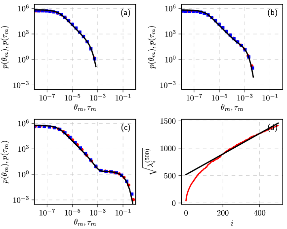
Figure 4: (color online) Burst and inter–burst duration PDFs ((a), (b) and (c)) for the Ornstein–Uhlenbeck process and square root of its eigenvalue spectrum (sub–figure (d)). In (a), (b) and (c) red circles represent numerical inter–burst duration PDF, blue squares represent numerical burst duration PDF, while black curve was obtained by evaluating Eq. (7). In (d) red curve represents a square roots of the eigenvalues, while black curve show the best linear fit. Parameters of the process were set as follows: (a) $N=10^{3}$, $h=0.45$ (for inter–burst duration) and $0.55$ (for burst duration), (b) $\varepsilon=1$, $N=10^{3}$, $h=0.5$ (for inter–burst and burst duration), (c) $N=10^{3}$, $h=0.55$ (for inter–burst duration) and $0.45$ (for burst duration), (d) was obtained with same parameters as (b).

4.3 The imitation process

Another birth–death process we consider in this paper is inspired by Kirman’s model [46]. This process is of particular interest, because it is known to exhibit long–range memory when applied to model financial markets [9]. The rates of this imitation process are given by:

$$\lambda_{k}^{+}=\left(N-X\right)\left(\varepsilon+X\right),\quad\lambda_{k}^{-}=X\left[\varepsilon+\left(N-X\right)\right].$$ (17)

This process can be interpreted as follows. $N$ agents switch between two states independently with rate $\varepsilon$ and also due to pairwise interactions, which happen at unit rate. Note that here we use simplified rates, while a more sophisticated forms can be also assumed to give the process a richer behavior [9].

In continuous limit from these rates we recover the following SDE:

$$\mathrm{d}x=\varepsilon\left(1-2x\right)\mathrm{d}t+\sqrt{2x(1-x)}\mathrm{d}W.$$ (18)

In Fig. 5 we show that burst and inter–burst durations in this model are indeed equivalent in statistical sense, as blue squares and red circles trace the same shape. Furthermore the approximation by Eq. (7) provides rather good approximation for that shape. Also in Fig. 5 (d) we show that the square root of the eigenvalue spectrum indeed grows linearly in a certain region.

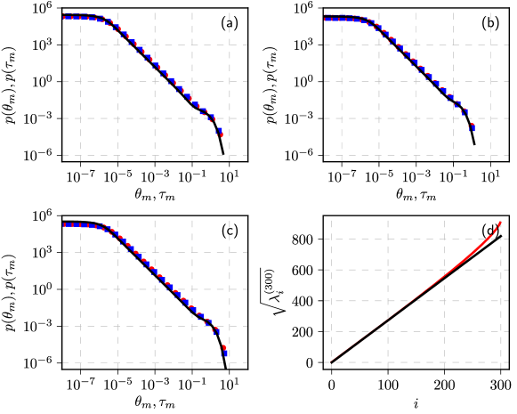
Figure 5: (color online) Burst and inter–burst duration PDFs ((a), (b) and (c)) for the imitation process and square root of its eigenvalue spectrum (sub–figure (d)). In (a), (b) and (c) red circles represent numerical inter–burst duration PDF, blue squares represent numerical burst duration PDF, while black curve was obtained by evaluating Eq. (7). In (d) red curve represents a square roots of the eigenvalues, while black curve show the best linear fit. Parameters of the process were set as follows: (a) $\varepsilon=0.5$, $N=10^{3}$, $h=0.3$ (for inter–burst duration) and $0.7$ (for burst duration), (b) $\varepsilon=1$, $N=10^{3}$, $h=0.2$ (for inter–burst duration) and $0.8$ (for burst duration), (c) $\varepsilon=1.5$, $N=10^{3}$, $h=0.7$ (for inter–burst duration) and $0.3$ (for burst duration), (d) was obtained with same parameters as (a).

5 Bursting statistics of the order book model exhibiting long–range memory

In this section we use Eq. (7) to fit bursting statistics obtained from the order book model exhibiting long–range memory [47]. From this model we have obtained numerical absolute return time series. We have treated the series using standard deviation filter with $10$ minute window as described in [38]. By setting the threshold level at $3$ standard deviations we have obtained burst and inter–burst duration PDFs, which are shown in Fig. 6 as red circles and blue squares.

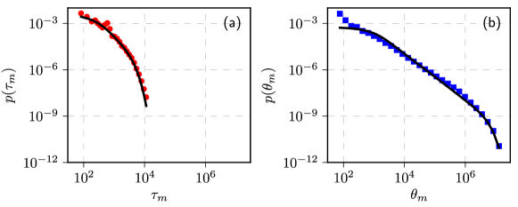
Figure 6: Burst (a) and inter–burst (b) duration PDFs of the numerical absolute return time series. Numerical absolute return time series were obtained by evaluating the order book model exhibiting long–range memory using parameter values fitting the statistical properties of Bitcoin time series best [47]. Threshold level was set at $3$ standard deviations of the numerical time series. Numerical burst duration PDF is given by red circles in (a) and numerical inter–burst duration PDF is given by blue squares in (b), while black curves provide the best fits according to Eq. (7). Parameters of the fits were set as follows: (a) $\rho=0.15$, $\lambda_{1}=9.1\cdot 10^{-4}$, $\lambda_{2}=8.4\cdot 10^{-3}$ and $\lambda_{m}=1.45\cdot 10^{-3}$, (b) $\rho=0.012$, $\lambda_{1}=5.1\cdot 10^{-7}$, $\lambda_{2}=9.4\cdot 10^{-7}$ and $\lambda_{m}=1.87\cdot 10^{-3}$.

As you can see in Fig. 6 the fit provided by black curves, which represent best fits according to Eq. (7), is rather good. The parameters of the fits were obtained by matching four empirical moments (mean, variance, third and fourth central moments) against the same moments calculated for Eq. (7). In both cases estimate of $\lambda_{m}$ was found to be reasonably close to $\frac{1}{600}$, which coincides with the standard deviation filter window we have used.

6 Conclusions

Here we have proposed a method to approximate the first passage time PDF between the successive states for any birth–death process. We have shown that the method works on a three distinct birth–death processes. As our derivation relies only on the general properties of birth–death process and on the concept of Riemann sum, we believe that the approximation should be applicable to any other birth–death process. Furthermore first passage times are invariant to variable transformations, thus the approximation method should be applicable to any one–dimensional diffusive process, which can be transformed into a birth–death process.

It is worth to note that our derivation suggests that all birth–death processes should share a peculiar property. The square root of their eigenvalue spectrum, $\sqrt{\lambda_{i}^{\left(n\right)}}$, should grow linearly for a wide range of ranks, $i$. This property must hold in order to be able to obtain power–law PDF with exponent $-3/2$, which is a known result for all one–dimensional Markov processes [31].

We have also used the proposed method to fit burst and inter–burst duration PDFs of the order book model exhibiting long–range memory [47]. This model is based on a birth–death process, but is significantly more sophisticated with other source of randomness embedded into the model. While this model is not a one–dimensional Markov process, but the approximation method seems to work reasonably well. This example is also particularly interesting, because it is able to reproduce power–law statistical properties of the Bitcoin time series. Including the presence of long–range memory. The fact that we are able to fit its burst and inter–burst duration PDFs suggests that the considered order book model exhibits spurious long–range memory, which could also be the nature of empirically observed long–range memory phenomenon. Indeed one could use a similar fitting method to fit the empirical burst and inter–burst duration PDFs. Yet to fully undertake the empirical fitting one first needs to find reliable methods to remove noise inherent to the empirical series.

References

- [1] A. L. Lloyd and R. M. May, “How viruses spread among computers and people,” Science, vol. 292, p. 1316, 2001.
- [2] M. C. Gonzalez, C. A. Hidalgo, and A. L. Barabasi, “Understanding individual human mobility patterns,” Science, vol. 453, p. 779, 2008.
- [3] V. Sundarapandian, Probability, Statistics and Qeueing Theory. New Delhi: PHI Learning Private Limited, 2009.
- [4] S. Alfarano and M. Milakovic, “Network structure and N-dependence in agent-based herding models,” Journal of Economic Dynamics and Control, vol. 33, no. 1, pp. 78–92, 2009.
- [5] A. Flache and M. W. Macy, “Local convergence and global diversity: From interpersonal to social influence,” Journal of Conflict Resolution, vol. 55, no. 6, pp. 970–995, 2011.
- [6] A. Kononovicius and J. Ruseckas, “Continuous transition from the extensive to the non-extensive statistics in an agent-based herding model,” European Physics Journal B, vol. 87, no. 8, p. 169, 2014.
- [7] R. Axelrod, “The dissemination of culture a model with local convergence and global polarization,” Journal of Conflict Resolution, vol. 41, no. 2, pp. 203–226, 1997.
- [8] A. Flache, M. Mas, T. Feliciani, E. Chattoe-Brown, G. Deffuant, S. Huet, and J. Lorenz, “Models of social influence: Towards the next frontiers,” The Journal of Artificial Society and Social Simulation, vol. 20, no. 4, p. 2, 2017.
- [9] A. Kononovicius and V. Gontis, “Agent based reasoning for the non-linear stochastic models of long-range memory,” Physica A, vol. 391, no. 4, pp. 1309–1314, 2012.
- [10] T. Kaizoji, M. Leiss, A. Saichev, and D. Sornette, “Super-exponential endogenous bubbles in an equilibrium model of fundamentalist and chartist traders,” Journal of Economic Behavior & Organization, vol. 112, pp. 289–310, 2015.
- [11] L. Cocco, G. Concas, and M. Marchesi, “Using an artificial financial market for studying a cryptocurrency market,” Journal of Economic Interaction and Coordination, vol. 12, no. 2, pp. 345–365, 2017.
- [12] A. E. Biondo, “Order book microstructure and policies for financial stability,” Studies in Economics and Finance, vol. 35, pp. 196–218, 2018.
- [13] R. Franke and F. Westerhoff, “Different compositions of animal spirits and their impact on macroeconomic stability.” Working Paper at University of Bamberg.
- [14] B. Llacay and G. Peffer, “Using realistic trading strategies in an agent-based stock market model,” Computational and Mathematical Organization Theory, vol. 24, no. 3, pp. 308–350, 2018.
- [15] B. Kaulakys, M. Alaburda, and J. Ruseckas, “1/f noise from the nonlinear transformations of the variables,” Modern Physics Letters B, vol. 29, no. 34, p. 1550223, 2015.
- [16] A. Kononovicius and J. Ruseckas, “Nonlinear GARCH model and 1/f noise,” Physica A, vol. 427, pp. 74–81, 2015.
- [17] M. Ding and W. Yang, “Distribution of the first return time in fractional Brownian motion and its application to the study of on-off intermittency,” Physical Review E, vol. 52, p. 207, 1995.
- [18] A. B. Dieker and M. Mandjes, “On spectral simulation of fractional Brownian motion,” Probability in the Engineering and Informational Sciences, vol. 17, no. 3, pp. 417–434, 2003.
- [19] K. E. Bassler, G. H. Gunaratne, and J. L. McCauley, “Markov processes, Hurst exponents, and nonlinear diffusion equations: With application to finance,” Physica A, vol. 369, no. 2, pp. 343–353, 2006.
- [20] J. L. McCauley, G. H. Gunaratne, and K. E. Bassler, “Hurst exponents, Markov processes, and fractional Brownian motion,” Physica A, vol. 379, no. 1, pp. 1 – 9, 2007.
- [21] J. L. McCauley, K. E. Bassler, and G. H. Gunaratne, “Martingales, detrending data, and the efficient market hypothesis,” Physica A, vol. 387, no. 1, pp. 202 – 216, 2008.
- [22] A. Kasprzak, R. Kutner, J. Perello, and J. Masoliver, “Higher-order phase transitions on financial markets,” The European Physical Journal B, vol. 76, p. 513, 2010.
- [23] R. Hilfer, “Mathematical analysis of time flow,” Analysis, vol. 36, no. 1, pp. 49–64, 2015.
- [24] M. Denys, M. Jagielski, T. Gubiec, R. Kutner, and H. E. Stanley, “Statistical collapse of excessive market losses,” Acta Physica Polonica A, vol. 129, no. 5, pp. 913–916, 2016.
- [25] M. O. Caceres, “On the quantum CTRW approach,” The European Physical Journal B, vol. 90, p. 74, 2017.
- [26] T. Gubiec and R. Kutner, “Continuous-Time Random Walk with multi-step memory: an application to market dynamics,” The European Physical Journal B, 2017.
- [27] R. Kutner and J. Masoliver, “The continuous time random walk, still trendy: fifty-year history, state of art and outlook,” The European Physical Journal B, vol. 90, p. 50, 2017.
- [28] L. Giraitis, R. Leipus, and D. Surgailis, “ARCH() models and long memory,” in Handbook of Financial Time Series (T. G. Anderson, R. A. Davis, J. Kreis, and T. Mikosh, eds.), pp. 71–84, Berlin: Springer Verlag, 2009.
- [29] L. Giraitis, H. L. Koul, and D. Surgailis, Large sample inference for long memory processes. World Scientific, 2012.
- [30] M. Tayefi and T. V. Ramanathan, “An overview of FIGARCH and related time series models,” Austrian Journal of Statistics, vol. 41, pp. 175–196, 2012.
- [31] S. Redner, A guide to first-passage processes. Cambridge University Press, 2001.
- [32] R. Metzler, G. Oshanin, and S. Redner, First-Passage Phenomena and Their Applications. Singapore: World Scientific, 2014.
- [33] A. N. Borodin and P. Salminen, Handbook of Brownian motion. Basel, Switzerland: Birkhauser, 2012.
- [34] J. Abate and W. Whitt, “A unified framework for numerically inverting Laplace transforms,” INFORMS Journal on Computing, vol. 18, no. 4, pp. 408–421, 2006.
- [35] V. Gontis, A. Kononovicius, and S. Reimann, “The class of nonlinear stochastic models as a background for the bursty behavior in financial markets,” Advances in Complex Systems, vol. 15, no. supp01, p. 1250071, 2012.
- [36] J. Ruseckas and B. Kaulakys, “1/f noise from nonlinear stochastic differential equations,” Physical Review E, vol. 81, p. 031105, 2010.
- [37] J. Keilson, “Markov chain models – rarity and exponentiality,” Applied Mathematical Sciences, vol. 28, 1979.
- [38] V. Gontis and A. Kononovicius, “Burst and inter-burst duration statistics as empirical test of long-range memory in the financial markets,” Physica A, vol. 483, pp. 266–272, 2017.
- [39] V. Gontis and A. Kononovicius, “Spurious memory in non-equilibrium stochastic models of imitative behavior,” Entropy, vol. 19, no. 8, p. 387, 2017.
- [40] V. Gontis and A. Kononovicius, “The consentaneous model of the financial markets exhibiting spurious nature of long-range memory,” Physica A, vol. 505, pp. 1075–1083, 2018.
- [41] J. Ruseckas and B. Kaulakys, “Tsallis distributions and 1/f noise from nonlinear stochastic differential equations,” Physical Review E, vol. 84, no. 5, p. 051125, 2011.
- [42] Y. Gong, Y.-H. Mao, and C. Zhang, “Hitting time distributions for denumerable birth and death processes,” Journal of Theoretical Probability, vol. 25, no. 4, pp. 950–980, 2012.
- [43] A. Dassios and L. Li, “Explicit asymptotics on first passage times of diffusion processes.” Available as arXiv:1806.08161 [math.PR].
- [44] O. Jouini and Y. Dallery, “Moments of first passage times in general birth-death processes,” Mathematical Methods of Operations Research, vol. 68, pp. 49–76, 2008.
- [45] M. Kounta, “First passage time of a Markov chain that converges to Bessel process,” Abstract and Applied Analysis, vol. 2017, p. 7189826, 2017.
- [46] A. P. Kirman, “Ants, rationality and recruitment,” Quarterly Journal of Economics, vol. 108, pp. 137–156, 1993.
- [47] A. Kononovicius and J. Ruseckas, “Order book model with herding behavior exhibiting long-range memory.” Available as arXiv: 1809.02772 [q-fin.ST].