Recycled Two-Stage Estimation in Nonlinear Mixed Effects Regression Models

Abstract

We consider a re-sampling scheme for estimation of the population parameters in the mixed effects nonlinear regression models of the type use for example in clinical pharmacokinetics, say. We provide an estimation procedure which recycles, via random weighting, the relevant two-stage parameters estimates to construct consistent estimates of the sampling distribution of the various estimates. We establish the asymptotic normality of the resampled estimates and demonstrate the applicability of the recycling approach in a small simulation study and via example.

Keywords: Bootstrapping; resampling; random weights; hierarchical nonlinear models; random effects.

1 Introduction

Hierarchical mixed-effects nonlinear regression models are widely used nowadays to analyze repeated measures observations. Data consisting of repeated measurements taken on each of a number of individuals arise commonly in biological and biomedical applications. Such models provide a natural settings for the analysis of data from pharmacokinetic studies obtained from a group of individuals which assumed to constitute a random sample from a relevant population of interest.

The hierarchical nonlinear model can be considered as an extension of the ordinary nonlinear regression models constructed to handle data obtained from several individuals. Modeling this kind of data usually involves a “functional” relationship between at least one of the predictor variables, $x$, and the measured response, $y$, within the individual’s data. As it often the case, the assumed ’functional’ model between the response $y$ and the predictor $x$, is based on some on physical or mechanistic grounds and is usually nonlinear in its parameters. These parameters are typically estimated from the data by some techniques suitable for nonlinear regression.

Figure 1 below shows drug concentration by time profiles for a study of the anti-asthmatic drug, Theophylline, as reported in Boeckmann, Sheiner and Beal (1994). Same dose of the drug was orally administered to 12 subjects, and over the subsequent 24 hour, serum concentrations were measured at ten time points per subject. For each subject, the pattern is of a rapid increase (post-drug) up to a to a peak concentration, followed by an apparent exponential decay. A common pharmacokinetics model to describe this relation following an oral administration of the Theophylline is the one-compartment model with first-order absorption and elimination rates (see for Example Davidian and Giltinan (1995)) .

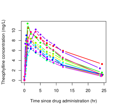
Figure 1: Drug concentrations for 12 participants in the Theophylline pharmacokinetics study

As we can see from this figure, this type of data involves within-subject variability as well as between-subject variability from an assumed population pharmacokinetic model. In such an hierarchical population model, fixed-effect parameters quantify the population average kinetics of the drug whereas inter-individual random effect parameters quantify the magnitude of inter-individual variability.

The basic hierarchical linear regression model was pioneered by Sheiner, Rosenberg and Melmon (1972), which accounted for both types of variations; of within and between subjects. The nonlinear case received widespread attention in later developments. Lindstrom and Bates (1990) proposed a general nonlinear mixed effects model for repeated measures data and proposed estimators combined least squares estimators and maximum likelihood estimators (under specific normality assumption). Vonesh and Carter (1992) discussed nonlinear mixed effects model for unbalanced repeated measures. Additional related references include: Mallet (1986), Davidian and Gallant (1993), Davidian and Giltinan (1993, 1995).

In all, the standard approach for statistical inference in hierarchical nonlinear models, is typically based on full distributional assumptions for both, the intra and inter individual random components. The most common assumption is that both random components are considered to be normally distributed. However, this can be a questionable assumption in many cases. Our main results in this work are built on more generalized assumptions in which the normally distributed random terms are not required.

One of the main approaches for estimation in such hierarchical ’population’ models is the two-stage estimation methods. At the first stage to estimate the ’individual’-level parameters and then to combine them by some manner to obtain the ’population’-level parameters. However, the main challenge to such two-stage estimation methods is to obtain the sampling distributions of the final estimators in order to evaluate performance, especially when there is no sufficient data available or whenever existing asymptotic results are not accurate. For most part, the performance of these estimation methods can only be evaluated empirically, primarily via the so-called Monte-Carlo simulations– see related references including: Sheiner and Beal (1981, 1982, 1983) and Davidian and Giltinan (1995, 2003). Hence, an alternate and more data oriented methodology should be considered. Bar-Lev and Boukai (2015) proposed a variant of the random weighting technique, which is termed herein recycling, as a valuable and valid alternative methodology for evaluation and comparison of the estimation procedure. Boukai and Zhang (2018) studied the asymptotic properties (asymptotic consistency and normality) of the recycled estimated in a one-layered nonlinear regression model.

In this paper we extend to the hierarchical nonlinear regression models the approach of Bar-Lev and Boukai (2015) to include general random weights and with minimal (only moments) assumptions on the random error-terms/effects. In Section 2, we introduce and study the standard two-stage (STS) estimates in the hierarchical settings of nonlinear mixed effect models, and establish the asymptotic consistency and asymptotic normality of the STS estimators in such general settings. As far as we know, these are the first provably valid asymptotic distributional results concerning the STS estimation procedure in the context of hierarchical nonlinear regression. Furthermore, in Section 3 we introduce a specialized re-sampling scheme to obtain the recycled version of the STS estimators and demonstrate their the asymptotic consistency and normality as well. The results of extensive simulation studies and a couple of detailed illustrations are provided in Section 4. The proofs of our main results along with many other technical details are provided in Section 5.

2 The Basic Hierarchical (Population) Model

Consider a study involving a random sample of $N$ individuals, where the nonlinear regression model (as in Boukai and Zhang (2018)) is assumed to hold for each of the $i$-th individuals. That is, for each $i$, $i=1,2,\dots,N$, we have available the $n_{i}$ (repeated) observations (with $n_{i}>p$) on the response variable in the form of ${\bf y}_{i}:=(y_{i1},y_{i2},\dots,y_{in_{i}})^{\bf t}$, where

$$y_{ij}=f({\bf x}_{ij};\,\bm{\theta}_{i})+\epsilon_{ij},\ \ \ \ j=1,\dots,n_{i},$$ (1)

and ${\bf x}_{ij}$ is the $j$-th fixed input (or condition) for the $i$-th individual, which gives rise to the response, $y_{ij}$, for $j=1,\dots,n_{i}$ and $i=1,\dots,N$. Here, $f(\cdot)$ is a given nonlinear function and $\epsilon_{ij}$ denote some $i.i.d.$ $(0,\sigma^{2})$ error-terms. That is, if we set ${\bm{\epsilon}}_{n_{i}}:=(\epsilon_{i1},\epsilon_{i2},\dots,\epsilon_{in_{i}})^{\bf t}$, then

$$E({\bm{\epsilon}}_{n_{i}})={\bf 0}\ \ \ \text{and}\ \ Var({\bm{\epsilon}}_{n_{i}})\equiv Cov({\bm{\epsilon}}_{n_{i}}{\bm{\epsilon}}^{\bf t}_{n_{i}})=\sigma^{2}\bf I_{n_{i}}.$$

In the current context, the parameter vector $\bm{\theta}=(\theta_{1},\theta_{2},\dots,\theta_{p})^{\bf t}\in\Theta\subset{I\!\!R}$ can vary from individual to individual, so that $\bm{\theta}_{i}$ is seen as the individual-specific realization of $\bm{\theta}$. More specifically, it is assumed that, independent of the error terms, ${\bm{\epsilon}}_{n_{i}}$,

$$\bm{\theta}_{i}:=\bm{\theta}_{0}+{\bf b}_{i},$$

where $\bm{\theta}_{0}:=(\theta_{01},\theta_{02},\dots,\theta_{0p})^{\bf t}$, is a fixed population parameter, though unknown, and ${\bf b}_{i}=(b_{i1},b_{i2},\dots,b_{ip})^{\bf t}$ is a $p\times 1$ vector representing the random effects associated with $i$-th individual. It is assumed that the random effects, ${\bf b}_{1},{\bf b}_{2},\dots,{\bf b}_{N}$ are independent and identically distributed random vectors satisfying,

$$E({\bf b}_{i})={\bf 0}\ \ \ \text{and}\ \ \ Var({\bf b}_{i})\equiv Cov({\bf b}_{i},{\bf b}_{i}^{t})={\bf D}.$$

Thus, $\bm{\theta}_{1},\bm{\theta}_{2},\dots,\bm{\theta}_{N}$ are $i.i.d.$ random vectors with

$$E(\bm{\theta}_{i})={\bf 0}\ \ \ \text{and}\ \ \ Var(\bm{\theta}_{i})={\bf D}.$$

In the simple hierarchical modeling it is often assumed that ${\bf D}$ is some diagonal matrix of the form ${\bf D}=Diag(\lambda_{1}^{2},\lambda_{2}^{2},\dots,\lambda_{p}^{2})$ or even simpler, as ${\bf D}=\lambda^{2}\bf I_{p}$ for some $\lambda>0$, and that both, the error terms ${\bm{\epsilon}}_{n_{i}}$, and the random effects ${\bf b}_{i}$ are normally distributed, so that,

$${\bm{\epsilon}}_{n_{i}}\sim{\cal N}_{n_{i}}({\bf 0},\sigma^{2}\bf I_{n_{i}}),\ \ \text{and}\ \ \ {\bf b}_{i}\sim{\cal N}_{p}({\bf 0},{\bf D}),$$

for each $=i=1,\dots,N$. In the more complex hierarchical modeling, more general structures of the within individual variability $Var({\bm{\epsilon}}_{n_{i}})=\Gamma_{i}$ (for some $\Gamma_{i}$) and of the between individuals variability, ${\bf D}$, are possible. However, even in the simplest structure, the available estimation methods for these model’s parameters, $\bm{\theta}_{0},\sigma^{2}$ and ${\bf D}$ are typically highly iterative in their nature and are based on the variations of the least squares estimation, and when available under some specific distributional assumptions, also on the maximum likelihood estimation procedures. In fact, many of the available results in the literature hinge on the specific normality assumption and on the ability to effectively ’linearize’ the regression function $f(\cdot)$ (see for example Bates and Watts (2007)). We point out that here we require no specific distributional assumptions (such as normality) on either ${\bm{\epsilon}}_{n_{i}}$ nor ${\bf b}_{i}$. However, we focus attention on the Standard Two Stage (STS) estimation procedure advocated by Steimer, Golmard and Boisvieux (1984).

3 The Two-Stage Estimation Procedure

For each $i=1,\dots,N$, let ${\bf f}_{i}(\bm{\theta})$ denote the $n_{i}\times 1$ vectors whose elements are $f({\bf x}_{ij},\bm{\theta}),j=1,\dots,n_{i}$ then model (1) can be written more succinctly as

$${\bf y}_{i}={\bf f}_{i}(\bm{\theta}_{i})+{\bm{\epsilon}}_{n_{i}}$$ (2)

Accordingly, the STS estimation procedure can be described as follows:

• On Stage I:   For each $i=1,\dots,N$ obtain $\hat{\bm{\theta}}_{ni}$ as the minimizer of

  $$Q_{i}(\bm{\theta}):=({\bf y}_{i}-{\bf f}_{i}(\bm{\theta}))({\bf y}_{i}-{\bf f}_{i}(\bm{\theta}))^{\bf t}\equiv\sum_{j=1}^{n_{i}}(y_{ij}-f({\bf x}_{ij},\bm{\theta}))^{2},$$ (3)

  so as to form $\hat{\bm{\theta}}_{n1},\hat{\bm{\theta}}_{n2},\dots,\hat{\bm{\theta}}_{nN}$, based on all the $M:=\sum_{i}^{N}n_{i}$ available observations. Next, estimate the within-individual variability component, $\sigma^{2}$, by

  $$\hat{\sigma}_{M}^{2}:=\frac{1}{M-pN}\sum_{i=1}^{N}Q_{i}({{\bm{{\hat{\theta}}_{n}}}_{i}}).$$

• On Stage II:   Estimate the ‘population’ parameter $\bm{\theta}_{0}$ by

  $$\bm{\hat{\theta}}_{{}_{STS}}:=\frac{1}{N}\sum_{i=1}^{N}{\bm{{\hat{\theta}}_{n}}}_{i}.$$ (4)

  Next, estimate $Var(\bm{\hat{\theta}}_{{}_{STS}})$ by ${\bf S}^{2}(\bm{\hat{\theta}})/N$, where

  $${\bf S}^{2}(\bm{\hat{\theta}}):=\sum_{i=1}^{N}({\bm{{\hat{\theta}}_{n}}}_{i}-\bm{\hat{\theta}}_{{}_{STS}})({\bm{{\hat{\theta}}_{n}}}_{i}-\bm{\hat{\theta}}_{{}_{STS}})^{\bf t}.$$

  Finally estimate the between-individual variability component, ${\bf D}$, by

  $$\bm{\hat{D}}={\bf S}^{2}(\bm{\hat{\theta}})-\min(\hat{\nu},\hat{\sigma}_{M}^{2}){\bm{\hat{\Sigma}}}_{N},$$ (5)

  where ${\bm{\hat{\Sigma}}}_{N}:=\frac{1}{N}\sum_{i=1}^{N}{\bm{\Sigma}}_{n_{i}}({\bm{{\hat{\theta}}_{n}}}_{i})$, with ${\bm{\Sigma}}^{-1}_{n_{i}}$ defined as,

  $$\bm{\Sigma}^{-1}_{n}(\bm{\theta}):=\frac{1}{n}\sum_{i=1}^{n}\nabla f_{i}(\bm{\theta})\nabla f_{i}(\bm{\theta})^{\bf t},$$ (6)

  and where $\hat{\nu}$ is the smallest root of the equation $|{\bf S}^{2}_{{}_{STS}}-\nu{\bm{\hat{\Sigma}}}_{N}|=0$, see Davidian and Giltinan (2003) for details.

Bar-Lev and Boukai (2015) provided a numerical study of this two-stage estimation procedure in the context of pharmacokinetics (hierarchical) modeling under the normality assumption. They also proposed a corresponding two-stage resampling (or recycling) algorithm, but based on ${\cal{D}}irichlet(\bm{1})$ random weights. However, in this paper we consider a more general framework for the random weights to be used.

For each $n\geq 1$, we let the random weights, ${\bf w}_{n}=(w_{1:n},w_{2:n},\dots,w_{n:n})^{\bf t}$, be a vector of exchangeable nonnegative random variables with $E(w_{i:n})=1$ and $Var(w_{i:n}):=\tau_{n}^{2}$, and let $W_{i}\equiv W_{1:n}=(w_{i:n}-1)/\tau_{n}$ be the standardized version of $w_{i:n}$, $i=1,\dots,n$. In addition we also assume, in similarity to Boukai and Zhang (2018) that,

Assumption W: The underlying distribution of the random weights ${\bf w}_{n}$ satisfies

1. For all $n\geq 1$, the random weights ${\bf w}_{n}$ are independent of $(\epsilon_{1},\epsilon_{2},\dots,\epsilon_{n})^{\bf t}$;

2. $\tau^{2}_{n}=o(n)$, $E(W_{i}W_{j})=O(n^{-1})$ and $E(W_{i}^{2}W_{j}^{2})\to 1$ for all $i\neq j$, $E(W_{i}^{4})<\infty$ for all $i$.

With such general random weights, the recycled version of the STS estimation procedure described in 3-6 above is:

• On Stage I^∗:   For each $i=1,\dots,N$, independently generate random weights, ${\bf w}_{i}=(w_{i1},w_{i2},\dots,w_{in_{i}})^{\bf t}$ that satisfy Assumption W with $Var(w_{ij})=\tau^{2}_{n_{i}}$ and obtain ${\bm{{\hat{\theta}}_{n}^{*}}}_{i}$ as the minimizer of

  $$Q_{i}^{*}(\bm{\theta}):=\sum_{j=1}^{n_{i}}w_{ij}(y_{ij}-f({\bf x}_{ij},\bm{\theta}))^{2},$$ (7)

  so as to form ${{\bm{{\hat{\theta}}_{n}^{*}}}_{1}},{\bm{{\hat{\theta}}_{n}^{*}}}_{2},\dots,{\bm{{\hat{\theta}}_{n}^{*}}}_{N}$.

• On Stage II^∗:  Independent of Step I^∗, generate random weights, ${\bf u}=(u_{1},u_{2},\dots,u_{N})^{\bf t}$ that satisfy Assumption W with $Var(u_{i})=\tau^{2}_{N}$, and obtained the recycled version of $\bm{\hat{\theta}}_{{}_{STS}}$ as:

  $$\bm{\hat{\theta}}_{{}_{STS}}^{*}:=\frac{1}{N}\sum_{i=1}^{N}u_{i}{\bm{{\hat{\theta}}_{n}^{*}}}_{i}$$ (8)

  The recycled version ${\bf D}^{*}$ of ${\bf D}$ can be subsequently obtained as described in Step II above.

4 Consistency of the Recycled STS Estimation Procedure

In this section we present some asymptotic results that establish and validate the consistency of the recycled STS estimator for general random weights satisfying the premises of Assumption W. We establish there results without the ’typical’ normality assumption on the within-individual error terms, $\epsilon_{ij}$, nor on the between-individual random effects ${\bf b}_{i}$. However, for simplicity of the exposition, we state these results in the case of $p=1$, so that $\Theta\in{I\!\!R}$. With that in mind, we denote for each $i=1,\dots,N$,

$$f_{ij}(\theta)\equiv f(x_{ij},\theta),\ \ \text{for}\ \ j=1,\dots,n_{i}.$$

Accordingly, the least squares criterion in (1), becomes

$$Q_{ni}(\theta):=\sum_{j=1}^{n_{i}}(y_{ij}-f_{ij}(\theta))^{2},$$

and the LS estimator $\hat{\theta}_{ni}$ is readily seen as the solution of

$$Q_{ni}^{\prime}(\theta):=2\sum_{j=1}^{n_{i}}\phi_{ij}(\theta)=0$$ (9)

where,

$$\phi_{ij}(\theta):=-(y_{ij}-f_{ij}(\theta))f^{{}^{\prime}}_{ij}(\theta),\ \ \ \$$ (10)

with $f^{{}^{\prime}}_{ij}(\theta):=df_{ij}(\theta)/d\theta$, for $j=1\dots,n_{i}$ and for each $i=1\dots,N$. We write $f^{{}^{\prime\prime}}_{ij}(\theta):=df^{\prime}_{ij}(\theta)/d\theta$ and $\phi^{\prime}_{ij}(\theta):=d\phi_{ij}(\theta)/d\theta$, etc. As in Boukai and Zhang (2018), we also assume that $f_{ij}^{{}^{\prime}}(\theta)$ and $f_{ij}^{{}^{\prime\prime}}(\theta)$ exist for all $\theta$ near $\theta_{0}$. However, to account for the inclusion of the $(0,\lambda^{2})$ random effect term, $b_{i}$, in the model, we also assume that,

Assumption A: For each $i=1,\dots,N$

1. $a_{n_{i}}^{2}:=\sigma^{2}\sum_{j=1}^{n_{i}}E(f^{{}^{\prime}2}_{ij}(\theta_{0}+b_{i}))\to\infty\ \ as\ \ n_{i}\to\infty$, ;

2. $\underset{n_{i}\to\infty}{\limsup}\ \ a_{n_{i}}^{-2}\sum_{j=1}^{n_{i}}\underset{|\theta-\theta_{0}-b_{i}|\leq\delta}{\sup}f_{ij}^{{}^{\prime\prime}2}(\theta)<\infty$

3. $a_{n_{i}}^{-2}\sum_{j=1}^{n_{i}}f_{ij}^{{}^{\prime}2}(\theta)\to\frac{1}{\sigma^{2}}$ uniformly in $|\theta-\theta_{0}-b_{i}|\leq\delta$.

In the following two Theorems we establish, under the conditions of Assumption A, the asymptotic consistency and normality of $\hat{\theta}_{{}_{STS}}$. Their proofs and some related technical results are given in Section 6.1 below.

Theorem 1

Suppose that Assumption A holds, then there exists a sequence $\hat{\theta}_{ni}$ of solutions of (9) such that

$$\hat{\theta}_{ni}=\theta_{0}+b_{i}+a_{ni}^{-1}T_{ni}$$

where $|T_{ni}|<K$ in probability, for each $i=1,2,\dots,N$. Further, there exists a sequence $\hat{\theta}_{{}_{STS}}$ as expressed in (4) such that

$$\hat{\theta}_{{}_{STS}}-\theta_{0}\overset{p}{\to}0,$$

as $n_{i}\to\infty$, for $i=1,2,\dots,N$, and as $N\to\infty$.

Theorem 2

Suppose that Assumption A holds. If

$$\underset{N,ni\to\infty}{\lim}N/a_{ni}^{2}<\infty,$$

for all $i=1,2,\dots,N$, then there exists a sequence $\hat{\theta}_{{}_{STS}}$ as expressed in (4) such that

$$\hat{\theta}_{{}_{STS}}-\theta_{0}=\frac{1}{N}\sum_{i=1}^{N}b_{i}-\psi_{{}_{N},n_{i}},$$

where $\sqrt{N}\psi_{{}_{N},n_{i}}\overset{p}{\to}0$ . Further,

$${\cal{R}_{N}}:=\frac{\sqrt{N}}{\lambda}(\hat{\theta}_{{}_{STS}}-\theta_{0})\Rightarrow{\cal N}(0,1)$$

as $n_{i}\to\infty$, for $i=1,2,\dots,N$, and as $N\to\infty$.

For the recycled STS estimation procedure as described in Section 3 above, the recycled version $\hat{\theta}^{*}_{ni}$ of $\hat{\theta}_{ni}$ is the minimizer of (7), or alternatively, the direct solution of

$$Q_{i}^{*\prime}(\theta):=2\sum_{j=1}^{n_{i}}w_{ij}\phi_{ij}(\theta)=0,$$ (11)

where ${\bf w}_{i}=(w_{i1},w_{i2},\dots,w_{in_{i}})^{\bf t}$ are the randomly drawn weights (satisfying Assumption W), for the $i$th individual, $i=1,2,\dots,N$. For establishing comparable results to those given in Theorems 1 and 2 for the recycled version, $\hat{\theta}^{*}_{{}_{STS}}=\sum_{i=1}^{N}u_{i}\hat{\theta}^{*}_{ni}/N$ of $\hat{\theta}_{{}_{STS}}=\sum_{i=1}^{N}\hat{\theta}_{ni}/N$, with the random weights ${\bf u}=(u_{1},u_{2},\dots,u_{N})^{\bf t}$ as in Stage II^∗, we need the following additional assumptions.

Assumption B: In addition to Assumption A, we assume that $E(\epsilon_{ij}^{4})<\infty$ and that for each $i=1,2,\dots,N$,

1. $\underset{n_{i}\to\infty}{\limsup}\ \ a_{n_{i}}^{-2}\sum_{j=1}^{n_{i}}\underset{|\theta-\theta_{0}-b_{i}|\leq\delta}{\sup}f_{ij}^{{}^{\prime}4}(\theta)<\infty$,

2. $\underset{n_{i}\to\infty}{\limsup}\ \ a_{n_{i}}^{-2}\sum_{j=1}^{n_{i}}\underset{|\theta-\theta_{0}-b_{i}|\leq\delta}{\sup}f_{ij}^{{}^{\prime\prime}4}(\theta)<\infty$,

3. As $n_{i}\to\infty$,   ${n_{i}}{a_{n_{i}}^{-2}}\to c_{i}\geq 0$ .

In Theorems 3 and 4 below we establish, under the conditions of Assumptions A and B, the asymptotic consistency and normality of the recycled estimator $\hat{\theta}^{*}_{{}_{STS}}$. Their proofs and some related technical results are given in Section 6.2 below.

Theorem 3

Suppose that Assumptions A and B hold. Then there exists a sequence $\hat{\theta}_{ni}^{*}$ as the solution of (11) such that

$$\hat{\theta}_{ni}^{*}=\hat{\theta}_{ni}+a_{ni}^{-1}T^{*}_{ni}$$

where $|T_{ni}^{*}|<K\tau_{n_{i}}$ in probability, for $i=1,\dots,N$. Further for any $\epsilon>0$, we have

$$P^{*}(|\hat{\theta}^{*}_{{}_{STS}}-\theta_{0}|>\epsilon)=o_{p}(1),$$

as $n_{i}\to\infty$, for $i=1,2,\dots,N$, and as $N\to\infty$.

Theorem 4

Suppose that Assumptions A and B hold. If for each $i=1,2,\dots,N$,

$$\frac{\tau_{n_{i}}}{\tau_{{}_{N}}}=o(\sqrt{n_{i}}),$$

then we have

$$\hat{\theta}^{*}_{{}_{STS}}-\hat{\theta}_{{}_{STS}}=\frac{1}{N}\sum_{i=1}^{N}(u_{i}-1)\hat{\theta}_{ni}-\psi^{*}_{{}_{N},n_{i}},$$

where $\frac{\sqrt{N}}{\tau_{{}_{N}}}\psi^{*}_{{}_{N},n_{i}}\overset{p^{*}}{\to}0$ as $N,n_{i}\to\infty$. Additionally,

$${\cal{R}^{*}_{N}}:=\frac{\sqrt{N}}{\lambda\tau_{{}_{N}}}(\hat{\theta}^{*}_{{}_{STS}}-\hat{\theta}_{{}_{STS}})\Rightarrow{\cal N}(0,1),$$

as $n_{i}\to\infty$, for $i=1,2,\dots,N$, and as $N\to\infty$.

The proofs of Theorems 3 and 4 and some related technical results are given in Section 6.2 below. The following corollary is an immediate consequence of the above results. It suggest that the sampling distribution of $\hat{\theta}_{{}_{STS}}$ can be well approximated by that of the recycled or re-sampled version of it, $\hat{\theta}^{*}_{{}_{STS}}$.

Corollary 5

For all $t\in I\!\!R$, let

$${\cal{H}}_{N}(t)=P\left({\cal{R}_{N}}\leq t\right),\ \ \ \text{and}\ \ \ \ {\cal{H}}_{N}^{*}(t)=P^{*}\left({\cal{R}^{*}_{N}}\leq t\right),$$

denote the corresponding c.d.f of ${\cal{R}_{N}}$ and ${\cal{R}^{*}_{N}}$, respectively. Then by Theorems 2 and 4,

$$\underset{t}{\sup}|{\cal{H}}_{n}^{*}(t)-{\cal{H}}_{n}(t)|\to 0\ \ \ in\ \ probability.$$

5 Implementation and Numerical Results

5.1 Illustrating the STS Estimation Procedure

To illustrate the main results of Section 4 for the hierarchical nonlinear regression model and the corresponding STS estimation procedure as described in 3-6 above, we consider a typical compartmental modeling from pharmacokinetics. In characterizing the pharmacokinetics of a drug disposition in the body, it is common to represent the body as a system of compartments and to assume that rates of transfer between compartments follow first-order or linear kinetics. Standard solution of the resulting differential equations shows that the relationship between drug concentration, as measured in the plasma and time (since administration of the drug to the body) may be described by a sum of exponential terms. For the standard two-compartment model, this relationship between the measure drug concentration $C(t)$ and the post-dosage time $t$, (following an intravenous administration), can be described through the nonlinear function of the form:

$$f(t;{\bm{\eta}})=Ae^{-\alpha t}+Be^{-\beta t},$$

with ${\bm{\eta}}:=(A,\alpha,B,\beta)^{\prime}$ is a parameter representing the various kinetics rate constants, such as the rate of elimination, rate of absorption, clearance, volume, etc. Since these constants (i.e. parameters) must be positive, we re-parametrize the model with $\bm{\theta}\equiv\log(\bm{\eta})$, so that with $t>0$,

$$f(t;\bm{\theta})=exp(\theta_{1})exp\{-exp(\theta_{2})t\}+exp(\theta_{3})exp\{-exp(\theta_{4})t\},$$ (12)

with $\bm{\theta}=(\theta_{1},\theta_{2},\theta_{3},\theta_{4})^{\bf t}\in{I\!\!R}^{4}$. For the simulation stdy we conducted here, we consider a situation in which the (plasma) drug concentrations $\{y_{ij}\}$ of $N$ individuals were measure at post-dose times $t_{ij}$ and are related as in model (1) via the nonlinear regression model,

$$y_{ij}=f(t_{ij};\bm{\theta}_{i})+\epsilon_{ij},$$

for $j=1,\dots,n_{i}$ and $i=1,\dots,N$. Here, as in Section 4, $\epsilon_{ij}$ are the standard $(0,\sigma^{2})$ error terms and $\bm{\theta}_{i}=\bm{\theta}_{0}+{\bf b}_{i}$, where $\bf{b}_{i}$ are independent identically distributed random effects terms, with mean $\bf{0}$ and unknown variance $\lambda^{2}{\bm{I}}_{4\times 4}$. Accordingly, we have in all a total of 6 unknown parameters, namely, $\bm{\theta}_{0}=(\theta_{10},\theta_{20},\theta_{30},\theta_{40})^{\bf t},\ \sigma$ and $\lambda$.

Since $\sigma$ and $\lambda$ represent variation within and between individuals (respectively), different setting for these two lead to very different situations. For instance, Figure 1(a) below, depicts the situation for $N=5$ and $n_{i}\equiv n=15$, each, when $\sigma=0.1$ and $\lambda=0.1$, so that the variation between individuals are similar to variation within individuals. Figure 1(b) depicts the situation with $\sigma=0.05,\lambda=1$, so that the variation between individuals is much larger than variation within individuals.

For the simulation, we set $\bm{\theta}_{0}=(1,0.8,-0.5,-1)^{\bf t}$, and for each $i$, the times $t_{ij},j=1,\dots,n$ were generated uniformly from $[0,8]$ interval. To allow for different ’distributions’, the error terms, $\epsilon_{ij}$, as well as the random effect terms, ${\bf b}_{i}$, were generated either from the (a) Truncated Normal, (b) Normal and (c) Laplace distributions – all in consideration of Assumption A in our main results.

For each simulation run, with the Truncated Normal distribution for the error-terms and the random effects terms, we calculated the value of $\hat{\bm{\theta}}^{k}_{{}_{STS}}$ as an estimator of $\bm{\theta}_{0}$ and repeated this procedure $M=1,000$ times to calculate the corresponding Mean Square Error (MSE) as followed,

$$MSE=\frac{1}{M}\sum_{k=1}^{M}||\hat{\bm{\theta}}^{k}_{{}_{STS}}-\bm{\theta}_{0}||^{2}$$

The corresponding simulation results obtained for various values of $N$ and $n$, are presented in Table 1 for $\sigma=0.1,\lambda=0.1$ and in Table 2 for $\sigma=0.05,\lambda=1$.

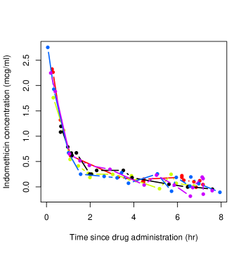
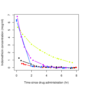
Figure 2: Drug plasma concentration vs time for (a) $\sigma=0.1,\lambda=0.1$; and for (b) $\sigma=0.05,\lambda=1$

	n=15	n=30	n=50	n=100	n=200
N=15	0.86616	0.22885	0.04651	0.01141	0.00632
N=30	0.57666	0.10713	0.02442	0.00573	0.00334
N=50	0.45840	0.08933	0.02097	0.00383	0.00195
N=100	0.37852	0.06918	0.01245	0.00216	0.00103
N=200	0.35059	0.05904	0.00891	0.00143	0.00058

Table 1: The MSE of STS estimates for truncated Normal error-terms/effects with $\sigma=0.1,\lambda=0.1$.

From these two table, we see that with $n$ and $N$ both increasing, the MSE is decreasing, as expected. However, $\sigma=0.05,\lambda=1$ as in Table 2, $n$ increasing for a fixed $N$, doesn’t contribute to smaller MSE, which is consistent with our main result Theorem 1, the STS estimate is not consistent with only $n_{i}\to\infty$, (this effect is more obvious in the case $\lambda$ is relatively large, as in the case of Table 2).

	n=15	n=30	n=50	n=100	n=200
N=15	1.00012	0.63825	0.56880	0.47304	0.46024
N=30	0.69974	0.39503	0.33145	0.35228	0.32632
N=50	0.55675	0.29437	0.25938	0.25004	0.23474
N=100	0.39821	0.22447	0.20213	0.19734	0.21995
N=200	0.34921	0.19447	0.17476	0.18824	0.19581

Table 2: The MSE of STS estimates for truncated Normal error-terms/effects with $\sigma=0.05,\lambda=1$.

For simulating the results of Theorem 2, we choose $\theta_{2}$ to be the unknown parameter, and use the main result to construct $95\%$ Confidence Interval as

$$(\hat{\theta}_{{}_{STS}}-1.96\frac{\hat{\lambda}}{\sqrt{N}},\ \hat{\theta}_{{}_{STS}}+1.96\frac{\hat{\lambda}}{\sqrt{N}}),$$

where

$$\hat{\lambda}^{2}=\frac{1}{N-1}\sum_{i=1}^{N}(\hat{\theta}_{ni}-\hat{\theta}_{{}_{STS}})^{2}.$$

The estimate for $\hat{\lambda}$ used here is the simple STS estimate, not the corrected one as in (5). M=1,000 replications of such simulations were executed to determine the percentage of times the true value of the parameter estimates was contained in the interval. We use $\sigma=0.5,\lambda=0.5$ and observed Coverage Percentages are provided in Table 3 below.

	n=15	n=30	n=50	n=100	n=200
N=15	0.903	0.934	0.933	0.931	0.931
N=30	0.896	0.940	0.940	0.943	0.944
N=50	0.883	0.941	0.959	0.944	0.944
N=100	0.828	0.948	0.946	0.941	0.944
N=200	0.759	0.943	0.932	0.935	0.949

Table 3: Coverage Percentage of the CI for the truncated Normal error-terms/effects with $\sigma=0.5,\lambda=0.5$.

From these results we can observe that with $n$ and $N$ both increase, the Coverage Percentage approximate to 0.95. While when $n$ is small (15), with $N$ increase, the Coverage Percentage is drifting farther away from the desired level of 0.95. This finding is consistent with our main result, the convergence require the condition $\underset{N,ni\to\infty}{\lim}N/a_{ni}^{2}<\infty$, which in this case becomes $\underset{n\to\infty}{\lim}\frac{1}{n}a_{n}^{2}/\sigma^{2}<\infty$, that is $\underset{N,n\to\infty}{\lim}N/n<\infty$ is required. Hence, when $N$ is much large than $n$, this condition does not hold. Although for this model, error terms that follow the normal distribution do not satisfy Assumption A, we used normal error terms in the simulations, and reported the resulting MSE and Coverage Percentage for 95% confidence interval is in Table 4 and Table 5. From the results we can observe that with $n$ and $N$ increasing, the MSE are smaller and Coverage Percentage are closer to 0.95.

	n=15	n=30	n=50	n=100	n=200
N=15	0.77176	0.17458	0.07880	0.01116	0.00615
N=30	0.55483	0.11852	0.02966	0.00605	0.00324
N=50	0.47721	0.09277	0.02164	0.00437	0.00195
N=100	0.38275	0.07416	0.01217	0.00231	0.00104
N=200	0.33843	0.05627	0.00892	0.00140	0.00059

Table 4: The MSE of STS estimates for Normal error-terms/effects with $\sigma=0.1,\lambda=0.1$.

	n=15	n=30	n=50	n=100	n=200
N=15	0.918	0.927	0.939	0.951	0.922
N=30	0.901	0.939	0.944	0.931	0.932
N=50	0.871	0.947	0.949	0.950	0.944
N=100	0.851	0.950	0.934	0.949	0.948
N=200	0.740	0.949	0.944	0.951	0.945

Table 5: Coverage Percentage of the CI for the Normal error-terms/effects with $\sigma=0.5,\lambda=0.5$.

We further considered simulations using the Laplace distributions for the error terms and random effects terms. The results are provided in Table 6 and Table 7. We can see the performance of STS estimates in Laplace error terms case is consistent with normal error case. We also illustrate the these simulation results in Figures 3 - 5. Figure 3 depicts the MSE of STS estimates for truncated Normal, Normal, Laplace error-terms/effects with $\sigma=0.1,\lambda=0.1$. Figure 4 depicts the MSE of STS estimates for truncated Normal error-terms/effects with $\sigma=0.05,\lambda=1$. Figure 5 illustrate the coverage percentage of the CI for the truncated Normal, Normal, Laplace error-terms/effects with $\sigma=0.5,\lambda=0.5$.

	n=15	n=30	n=50	n=100	n=200
N=15	1.03613	0.38643	0.12267	0.03157	0.01450
N=30	0.73469	0.23642	0.06831	0.01897	0.00756
N=50	0.63382	0.18683	0.04771	0.01161	0.00492
N=100	0.50973	0.14164	0.03378	0.00738	0.00288
N=200	0.48408	0.11612	0.02806	0.00532	0.00159

Table 6: The MSE of STS estimates for Laplace error-terms/effects with $\sigma=0.1,\lambda=0.1$.

	n=15	n=30	n=50	n=100	n=200
N=15	0.878	0.908	0.932	0.936	0.944
N=30	0.830	0.922	0.943	0.935	0.946
N=50	0.791	0.920	0.950	0.947	0.945
N=100	0.669	0.927	0.933	0.946	0.942
N=200	0.455	0.893	0.945	0.932	0.951

Table 7: Coverage Percentage of the CI for the Laplace error-terms/effects with $\sigma=0.5,\lambda=0.5$.

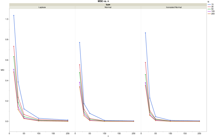
Figure 3: The MSE of STS estimates for truncated Normal, Normal, Laplace error-terms/effects with $\sigma=0.1,\lambda=0.1$.

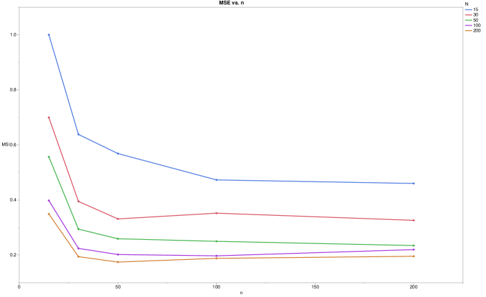
Figure 4: The MSE of STS estimates for truncated Normal error-terms/effects with $\sigma=0.05,\lambda=1$.

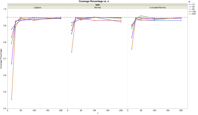
Figure 5: Coverage Percentage of the CI for the truncated Normal, Normal, Laplace error-terms/effects with $\sigma=0.5,\lambda=0.5$.

5.2 Illustrating the Recycled STS Estimation Procedure

In this section, we provide the results of the simulation studies corresponding to Theorem 3 and 4 concerning the recycled STS estimation procedure with $\hat{\theta}^{*}_{{}_{STS}}$. We considered the same compartmental model as given in the previous subsection, however again with $p=1$. Accordingly, we choose $\theta_{2}$ to represent the model’s unknown parameter and set, for the simulations, $\theta_{0}=0.8$, for each $i$. As before, we generated the values of $\{t_{ij},j=1,\dots,n\}$ uniformly from the $[0,8]$ interval, and draw the error terms, $\epsilon_{ij}$ and the random effects terms, $b_{i}$, from the truncated Normal distribution.

For each simulation run, we calculated the value of $\hat{\theta}_{{}_{STS}}$ as in section 4.2, then with $B=1,000$, we generated $B\times N$ independent replications of the random weights ${\bf w}_{i}=(w_{i1},w_{i2},\dots,w_{in})$ and $B=1,000$ independent replications of the random weight ${\bf u}=(u_{1},u_{2},\dots,u_{N})$, to obtain $\hat{\theta}^{*1}_{{}_{STS}}$, $\hat{\theta}^{*2}_{{}_{STS}}$, $\dots$, $\hat{\theta}^{*B}_{{}_{STS}}$. The correspond 95% Confidence Intervals were formed. With $\sigma=1$, $\lambda=1$ a total of $M=2000$ replications of such simulations were executed to determine the percentage of times the true value of the parameter estimates was contained in the interval and average confidence interval length was calculated. The Coverage Percentages with average confidence interval lengths are provided in Table 8 to Table 11.

Table 8 demonstrates the results of the asymptotic results of Section 4. Table 9 to 11 provide Coverage Percentages with average confidence interval lengths, with random weights set to be Multinomial, Dirichlet or Exponential distributed . From these results we can see with $N$ and $n$ both increase, the Coverage Percentages converges to 0.95 as expected. Also notice that Coverage Percentages derived from the recycled STS are more accurate (closer to 0.95) than the asymptotic result, especially when $n$ and $N$ are small.

	n=15	n=30	n=50	n=100
N=15	0.755	0.880	0.905	0.920
	0.999	1.004	1.009	1.038
N=30	0.590	0.860	0.930	0.955
	0.730	0.722	0.729	0.740
N=50	0.48	0.815	0.885	0.955
	0.566	0.576	0.568	0.573
N=100	0.170	0.680	0.895	0.935
	0.397	0.403	0.410	0.406

Table 8: Simulated Coverage Percentage of the CI for the truncated Normal error-terms/effects with $\sigma=1,\lambda=1$.

	n=15	n=30	n=50	n=100
N=15	0.860	0.910	0.930	0.940
	1.222	1.191	1.179	1.170
N=30	0.780	0.915	0.955	0.960
	0.881	0.855	0.851	0.832
N=50	0.760	0.890	0.940	0.940
	0.787	0.683	0.660	0.648
N=100	0.500	0.850	0.935	0.945
	0.478	0.473	0.471	0.458

Table 9: Coverage Percentage of the CI for the truncated Normal error-terms/effects with $\sigma=1,\lambda=1$ and with Multinomial random weights.

	n=15	n=30	n=50	n=100
N=15	0.810	0.905	0.930	0.950
	1.303	1.362	1.364	1.407
N=30	0.695	0.900	0.955	0.965
	0.936	0.965	0.993	1.001
N=50	0.605	0.870	0.930	0.965
	0.725	0.761	0.766	0.773
N=100	0.305	0.795	0.935	0.950
	0.509	0.534	0.550	0.546

Table 10: Coverage Percentage of the CI for the truncated Normal error-terms/effects with $\sigma=1,\lambda=1$ and with Dirichlet random weights.

	n=15	n=30	n=50	n=100
N=15	0.810	0.895	0.920	0.945
	1.296	1.351	1.347	1.397
N=30	0.680	0.890	0.960	0.965
	0.935	0.965	0.990	0.999
N=50	0.590	0.855	0.930	0.940
	0.729	0.765	0.765	0.771
N=100	0.300	0.805	0.935	0.950
	0.507	0.532	0.550	0.546

Table 11: Coverage Percentage of the CI for the truncated Normal error-terms/effects with $\sigma=1,\lambda=1$ and with Exponential random weights.

To complement of the simulations, we also considered the Laplace distribution for the error and random effects terms and present the corresponding simulation results Tables 12 - 15, below. Table 12 demonstrates the results from asymptotic result as in Section 4. Table 13 to 15 present Coverage Percentages with average confidence interval lengths with weights set to be according to the Multinomial, Dirichlet and the Exponential distributions. The results have similar performance as in normal random component case. Also notice that Coverage Percentages derived from the recycled STS method are also more accurate (closer to 0.95) than the asymptotic result, especially for smaller $n$ and $N$.. We also illustrate these simulation results in Figure 6 and 7. Figure 6 is coverage percentage of the CI for the truncated Normal error-terms/effects with $\sigma=1,\lambda=1$. Figure 7 is average length of the CI for the truncated Normal error-terms/effects with $\sigma=1,\lambda=1$. From this figure we can observe that with an increasing $N$, the average length of the CI is decreasing, however, with only $n$ increase the length will not decrease, which is consistent with our main results.

	n=15	n=30	n=50	n=100
N=15	0.790	0.895	0.910	0.895
	0.998	0.974	0.964	1.007
N=30	0.730	0.885	0.870	0.940
	0.714	0.726	0.715	0.714
N=50	0.475	0.840	0.925	0.940
	0.559	0.562	0.546	0.552
N=100	0.220	0.715	0.895	0.960
	0.395	0.388	0.390	0.397

Table 12: Simulated Coverage Percentage of the CI for the Laplace error-terms/effects with $\sigma=1,\lambda=1$.

	n=15	n=30	n=50	n=100
N=15	0.885	0.935	0.950	0.950
	1.205	1.182	1.160	1.171
N=30	0.905	0.960	0.915	0.955
	0.865	0.854	0.846	0.815
N=50	0.760	0.930	0.965	0.960
	0.677	0.670	0.653	0.637
N=100	0.620	0.825	0.935	0.965
	0.475	0.465	0.459	0.456

Table 13: Coverage Percentage of the CI for the Laplace error-terms/effects with $\sigma=1,\lambda=1$ and with Multinomial random weights.

	n=15	n=30	n=50	n=100
N=15	0.830	0.930	0.960	0.965
	1.309	1.350	1.367	1.422
N=30	0.815	0.935	0.910	0.965
	0.926	0.974	0.984	0.980
N=50	0.615	0.915	0.965	0.965
	0.721	0.758	0.757	0.768
N=100	0.440	0.800	0.940	0.985
	0.508	0.528	0.537	0.546

Table 14: Coverage Percentage of the CI for the Laplace error-terms/effects with $\sigma=1,\lambda=1$ and with Dirichlet random weights.

	n=15	n=30	n=50	n=100
N=15	0.845	0.930	0.950	0.960
	1.302	1.334	1.355	1.407
N=30	0.820	0.940	0.935	0.965
	0.923	0.969	0.982	0.979
N=50	0.600	0.910	0.965	0.955
	0.717	0.757	0.757	0.764
N=100	0.435	0.815	0.945	0.985
	0.507	0.526	0.537	0.544

Table 15: Coverage Percentage of the CI for the Laplace error-terms/effects with $\sigma=1,\lambda=1$ and with Exponential random weights.

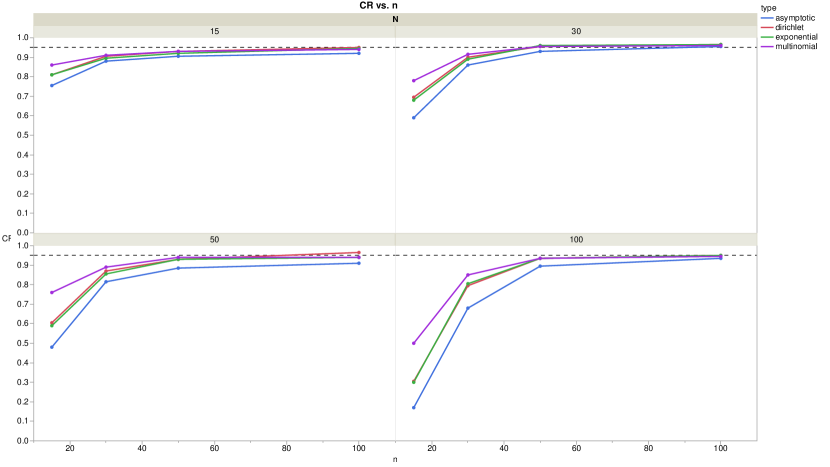
Figure 6: Coverage Percentage of the CI for the truncated Normal error-terms/effects with $\sigma=1,\lambda=1$.

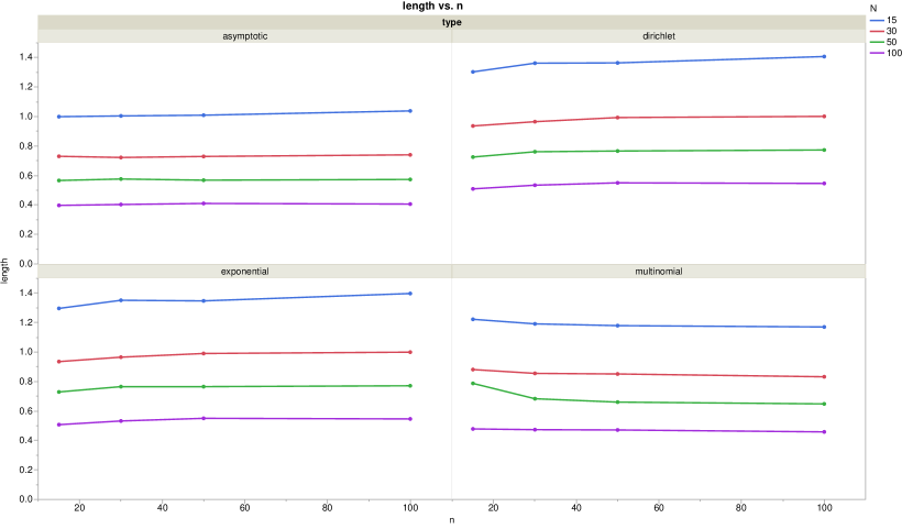
Figure 7: Average length of the CI for the truncated Normal error-terms/effects with $\sigma=1,\lambda=1$.

6 Technical Details and Proofs

6.1 Technical Details and Proofs – the STS Estimation Case

In this section we provide the technical results needed for the proofs of Theorems 1 and 2 on the STS estimator $\hat{\theta}_{{}_{STS}}$ in the hierarchical nonlinear regression model. In the sequel, we let $\phi_{1ij}(\theta):=\phi_{ij}^{{}^{\prime}}(\theta)$ (see (10)), and set $K$ to denote a generic constant. Recall that (see Assumption A(1)),

$$a_{n_{i}}^{2}:=\sigma^{2}\sum_{j=1}^{n_{i}}E(f^{{}^{\prime}2}_{ij}(\theta_{0}+b_{i}))\to\infty\ \ as\ \ n_{i}\to\infty.$$

Lemma 1

Under the conditions of Assumption A, for some $K>0$

$$a_{n_{i}}^{-2}\underset{|t|\leq K}{\sup}\sum_{j=1}^{n_{i}}\phi_{1ij}(b_{i1})-\frac{1}{\sigma^{2}}\to 0\ \ a.s.,$$

where $b_{i1}:=b_{1n_{i}}(t)$ is a sequence such that $\underset{|t|\leq K}{\sup}|b_{i1}-b_{i}-\theta_{0}|\to 0,\ \ \ a.s.,$ as $n_{i}\to\infty$.

Proof of Lemma 1: Since $\phi_{1ij}(\theta):=\phi_{ij}^{{}^{\prime}}(\theta)$, we have

$$\phi_{1ij}(\theta)\equiv f^{{}^{\prime}2}_{ij}(\theta)-\epsilon_{ij}f_{ij}^{{}^{\prime\prime}}(\theta)-(f_{ij}(\theta_{0}+b_{i})-f_{ij}(\theta))f_{ij}^{{}^{\prime\prime}}(\theta).$$

Accordingly, we first note that,

$$\left|a_{n_{i}}^{-2}\underset{|t|\leq K}{\sup}\sum_{j=1}^{n_{i}}\phi_{1ij}(b_{i1})-\frac{1}{\sigma^{2}}\right| \leq \left|a_{n_{i}}^{-2}\underset{|t|\leq K}{\sup}\sum_{j=1}^{n_{i}}f^{{}^{\prime}2}_{ij}(b_{i1})-\frac{1}{\sigma^{2}}\right|$$

$$+ a_{n_{i}}^{-2}\underset{|t|\leq K}{\sup}\left|\sum_{j=1}^{n_{i}}\epsilon_{ij}f_{ij}^{{}^{\prime\prime}}(b_{i1})\right|$$

$$+ a_{n_{i}}^{-2}\underset{|t|\leq K}{\sup}\left|\sum_{j=1}^{n_{i}}(f_{ij}(\theta_{0}+b_{i})-f_{ij}(b_{i1}))f_{ij}^{{}^{\prime\prime}}(b_{i1})\right|.$$

By Assumption A $(3)$, we have $a_{n_{i}}^{-2}\underset{|t|\leq K}{\sup}\sum_{j=1}^{n_{i}}f^{{}^{\prime}2}_{ij}(b_{i1})-\frac{1}{\sigma^{2}}\to 0\ \ a.s.,$ and by Assumption A $(2)$ and Corollary A in Wu (1981), we also have,

$$a_{n_{i}}^{-2}\underset{|t|\leq K}{\sup}\left|\sum_{j=1}^{n_{i}}\epsilon_{ij}f_{ij}^{{}^{\prime\prime}}(b_{i1})\right|\to 0\ \ a.s..$$

Finally, the last term converge to $0$ a.s. by Assumption A, an application of Cauchy-Schwarz inequality and Corollary A in Wu (1981). Thus we have

$$a_{n_{i}}^{-2}\underset{|t|\leq K}{\sup}\sum_{j=1}^{n_{i}}\phi_{1ij}(b_{i1})-\frac{1}{\sigma^{2}}\to 0\ \ a.s..$$

. Q.E.D.

Lemma 2

Let $X_{i}$ be a sequence of random variables bounded in probability and let $Y_{i}$ be a sequence of random variables which satisfies $\frac{1}{n}\sum_{i=1}^{n}|Y_{i}|\to 0$ in probability. Then $\frac{1}{n}\sum_{i=1}^{n}X_{i}Y_{i}\overset{p}{\to}0.$

Proof of Lemma 2: Since $X_{i}$ is bounded in probability, for any $\epsilon>0$, there is $K_{\epsilon}$ such that with sufficient large i, $P(|X_{i}|>K_{\epsilon})<\epsilon.$ Then

$$\underset{n\to\infty}{\lim}P(|\frac{1}{n}\sum_{i=1}^{n}X_{i}Y_{i}|>\epsilon) = \underset{n\to\infty}{\lim}\left[P(|\frac{1}{n}\sum_{i=1}^{n}X_{i}Y_{i}|>\epsilon,|X_{i}|<K_{\epsilon})\right]$$

$$+ \underset{n\to\infty}{\lim}\left[P(|\frac{1}{n}\sum_{i=1}^{n}X_{i}Y_{i}|>\epsilon,|X_{i}|>K_{\epsilon})\right]$$

$$\leq \underset{n\to\infty}{\lim}P(\frac{1}{n}\sum_{i=1}^{n}|\frac{X_{i}}{K_{\epsilon}}Y_{i}|>\frac{\epsilon}{K_{\epsilon}},|X_{i}|<K_{\epsilon})+\epsilon$$

$$\leq \underset{n\to\infty}{\lim}P(\frac{1}{n}\sum_{i=1}^{n}|Y_{i}|>\frac{\epsilon}{K_{\epsilon}},|X_{i}|<K_{\epsilon})+\epsilon=\epsilon,$$

from which the desired result follows. Q.E.D.

Lemma 3

There exists a $K>0$ such that for any $\epsilon>0$, for any $i$,

$$P\left[\left|a_{n_{i}}^{-1}\sum_{j=1}^{n_{i}}\phi_{ij}(\theta_{0}+b_{i})\right|>K\right]<\frac{\epsilon}{2}.$$

Proof of Lemma 3: Since $\epsilon_{ij}$ and $b_{i}$ are independent, for each $i=1,\dots,N$, we have that for any $j_{1}\neq j_{2}$,

$$E(\phi_{ij_{1}}(\theta_{0}+b_{i})\phi_{ij_{2}}(\theta_{0}+b_{i})) = E[E(\phi_{ij_{1}}(\theta_{0}+b_{i})\phi_{ij_{2}}(\theta_{0}+b_{i})|b_{i})]$$

$$= E[E(\epsilon_{ij_{1}}\epsilon_{ij_{2}}f^{{}^{\prime}}_{ij_{1}}(\theta_{0}+b_{i})f^{{}^{\prime}}_{ij_{2}}(\theta_{0}+b_{i})|b_{i})]$$

$$= E[E(\epsilon_{ij_{1}})E(\epsilon_{ij_{2}})f^{{}^{\prime}}_{ij_{1}}(\theta_{0}+b_{i})f^{{}^{\prime}}_{ij_{2}}(\theta_{0}+b_{i})]$$

$$= 0.$$

Similarly,

$$E(\phi_{ij_{1}}(\theta_{0}+b_{i})) = E[E(\epsilon_{ij_{1}}f^{{}^{\prime}}_{ij_{1}}(\theta_{0}+b_{i})|b_{i})]$$

$$= E[E(\epsilon_{ij_{1}})f^{{}^{\prime}}_{ij_{1}}(\theta_{0}+b_{i})]$$

$$= 0.$$

Hence, we have,

$$E(\phi_{ij_{1}}(\theta_{0}+b_{i})\phi_{ij_{2}}(\theta_{0}+b_{i}))=E(\phi_{ij_{1}}(\theta_{0}+b_{i}))E(\phi_{ij_{2}}(\theta_{0}+b_{i})).$$

To conclude that,

$$Var\left(\sum_{j=1}^{n_{i}}\phi_{ij}(\theta_{0}+b_{i})\right) = \sum_{j=1}^{n_{i}}Var(\phi_{ij}(\theta_{0}+b_{i}))$$

$$= \sum_{j=1}^{n_{i}}Var(\epsilon_{ij}f^{{}^{\prime}}_{ij}(\theta_{0}+b_{i}))$$

$$= \sum_{j=1}^{n_{i}}E(\epsilon^{2}_{ij})E(f^{{}^{\prime}2}_{ij}(\theta_{0}+b_{i}))$$

$$= \sigma^{2}\sum_{j=1}^{n_{i}}E(f^{{}^{\prime}2}_{ij}(\theta_{0}+b_{i}))\equiv a_{n_{i}}^{2}.$$

Accordingly, there exists a $K>0$ such that for any $\epsilon>0$, for any $i$,

$$P\left[\left|a_{n_{i}}^{-1}\sum_{j=1}^{n_{i}}\phi_{ij}(\theta_{0}+b_{i})\right|>K\right]<\frac{\epsilon}{2}.$$

Q.E.D.

Proof of Theorem 1: Let

$$S_{n_{i}}(t):=a_{n_{i}}^{-1}\sum_{j=1}^{n_{i}}\left[\phi_{ij}(\theta_{0}+b_{i}+a_{n_{i}}^{-1}t)-\phi_{ij}(\theta_{0}+b_{i})\right]-\frac{t}{\sigma^{2}}.$$ (13)

Next we will show for any given constant $K$,

$$\underset{|t|\leq K}{sup}|S_{n_{i}}(t)|\to 0\ \ a.s.$$ (14)

By a Taylor expansion, $\phi_{ij}(\theta_{0}+b_{i}+a_{n_{i}}^{-1}t)=\phi_{ij}(\theta_{0}+b_{i})+\phi_{1ij}(b_{i1})a_{n_{i}}^{-1}t,\ \$ where $b_{i1}=\theta_{0}+b_{i}+ca_{n_{i}}^{-1}t$ for some $0<c<1$. Accordingly we obtain that,

$$\underset{|t|\leq K}{\sup}|S_{n_{i}}(t)| = \underset{|t|\leq K}{\sup}\left|a_{n_{i}}^{-1}\sum_{j=1}^{n_{i}}\phi_{1ij}(b_{i1})a_{n_{i}}^{-1}t-\frac{t}{\sigma^{2}}\right|$$

$$= K\left|a_{n_{i}}^{-2}\underset{|t|\leq K}{\sup}\sum_{j=1}^{n_{i}}\phi_{1ij}(b_{i1})-\frac{1}{\sigma^{2}}\right|.$$

By Lemma 1, $a_{n_{i}}^{-2}\underset{|t|\leq K}{\sup}\sum_{j=1}^{n_{i}}\phi_{1ij}(b_{i1})-\frac{1}{\sigma^{2}}\to 0\ \ a.s.$ Thus, we have proved (14). Next, by (13),

$$A_{n_{i}}(t):=a_{n_{i}}^{-1}t\sum_{j=1}^{n_{i}}\phi_{ij}(\theta_{0}+b_{i}+a_{n_{i}}^{-1}t)=tS_{n_{i}}(t)+a_{n_{i}}^{-1}t\sum_{j=1}^{n_{i}}\phi_{ij}(\theta_{0}+b_{i})+\frac{t^{2}}{\sigma^{2}}.$$

Thus,

$$\underset{|t|=K}{\inf}A_{n_{i}}(t)\geq-K\underset{|t|=K}{\sup}|S_{n_{i}}(t)|-Ka_{n_{i}}^{-1}\left|\sum_{j=1}^{n_{i}}\phi_{ij}(\theta_{0}+b_{i})\right|+\frac{K^{2}}{\sigma^{2}}.$$

By lemma 3 there exists a $K>0$ such that for any $\epsilon>0$, for any $i$,

$$P\left[\left|a_{n_{i}}^{-1}\sum_{j=1}^{n_{i}}\phi_{ij}(\theta_{0}+b_{i})\right|>K\right]<\frac{\epsilon}{2}.$$ (15)

So that by (15) and (14) we may choose $K$ large enough such that for sufficiently large $n_{i}$,

$$P(\underset{|t|=K}{\inf}A_{n_{i}}(t)\geq 0) \geq P(\underset{|t|=K}{\sup}|S_{n_{i}}(t)|+a_{n_{i}}^{-1}\left|\sum_{j=1}^{n_{i}}\phi_{ij}(\theta_{0}+b_{i})\right|\leq\frac{K}{\sigma^{2}})$$

$$= 1-P(\underset{|t|=K}{\sup}|S_{n_{i}}(t)|+a_{n_{i}}^{-1}\left|\sum_{j=1}^{n_{i}}\phi_{ij}(\theta_{0}+b_{i})\right|>\frac{K}{\sigma^{2}})$$

$$\geq 1-P(\underset{|t|=K}{\sup}|S_{n_{i}}(t)|>\frac{K}{4\sigma^{2}})-P(a_{n_{i}}^{-1}\left|\sum_{j=1}^{n_{i}}\phi_{ij}(\theta_{0}+b_{i})\right|>\frac{K}{4\sigma^{2}})$$

$$\geq 1-\epsilon.$$

By the continuity of $\sum_{j=1}^{n_{i}}\phi_{ij}(\theta)$ in $\theta$, we have, for sufficiently large $n_{i}$, that there exists a constant $K$ such that the equation

$$\sum_{j=1}^{n_{i}}\phi_{ij}(\theta_{0}+b_{i}+a_{n_{i}}^{-1}t)=0,$$

has a root $t=T_{ni}$ in $|t|\leq K$ with probability larger than $1-\epsilon$. That is, we have

$$\hat{\theta}_{ni}=\theta_{0}+b_{i}+a_{ni}^{-1}T_{ni},$$

where $|T_{ni}|<K$ in probability. Thus, by Lemma 2,

$$\hat{\theta}_{{}_{STS}}-\theta_{0}=\frac{1}{N}\sum_{i=1}^{N}b_{i}+\frac{1}{N}\sum_{i=1}^{N}a_{ni}^{-1}T_{ni}\overset{p}{\to}0.$$

Q.E.D.

For establishing the asymptotic normality result as stated in Theorem 2, we need the following Lemma.

Lemma 4

Under the conditions of Assumptions A,

$$\frac{1}{\sqrt{N}}\sum_{i=1}^{N}a_{n_{i}}^{-2}\sum_{j=1}^{n_{i}}\phi_{ij}(\theta_{0}+b_{i})\overset{p}{\to}0.$$

Proof of Lemma 4: Let $X_{ni}:=a_{n_{i}}^{-1}\sum_{j=1}^{n_{i}}\phi_{ij}(\theta_{0}+b_{i}),$ where, by proof of Theorem 1 we have $E(X_{ni})=0$ and $Var(X_{ni})=1$. Thus,

$$\frac{1}{\sqrt{N}}\sum_{i=1}^{N}a_{n_{i}}^{-2}\sum_{j=1}^{n_{i}}\phi_{ij}(\theta_{0}+b_{i})=\frac{1}{\sqrt{N}}\sum_{i=1}^{N}a_{n_{i}}^{-1}X_{ni}.$$

Now, for any $\epsilon>0$,

$$P(\left|\frac{1}{\sqrt{N}}\sum_{i=1}^{N}a_{n_{i}}^{-1}X_{ni}\right|>\epsilon)\leq\frac{\sum_{i=1}^{N}\frac{1}{a_{ni}^{2}}}{N\epsilon^{2}}\to 0.$$

Accordingly, we have $\frac{1}{\sqrt{N}}\sum_{i=1}^{N}a_{n_{i}}^{-2}\sum_{j=1}^{n_{i}}\phi_{ij}(\theta_{0}+b_{i})\overset{p}{\to}0,$ as required. Q.E.D.

Proof of Theorem 2: We first note that by Lemma 1 and (13),

$$\hat{\theta}_{ni}-\theta_{0}-b_{i}=-a_{ni}^{-2}\sigma^{2}\sum_{j=1}^{n_{i}}\phi_{ij}(\theta_{0}+b_{i})-a_{n_{i}}^{-1}\sigma^{2}S_{n_{i}}(T_{ni}).$$

Thus,

$$\hat{\theta}_{{}_{STS}}-\theta_{0}=\frac{1}{N}\sum_{i=1}^{N}b_{i}-\frac{\sigma^{2}}{N}\sum_{i=1}^{N}a_{n_{i}}^{-2}\sum_{j=1}^{n_{i}}\phi_{ij}(\theta_{0}+b_{i})-\frac{\sigma^{2}}{N}\sum_{i=1}^{N}a_{n_{i}}^{-1}S_{n_{i}}(T_{ni}).$$

Recall that $\sum_{i=1}^{N}b_{i}/N\to E(b_{1})\equiv 0$. In view of (14) and since, $\underset{N,ni\to\infty}{\lim}N/a_{ni}^{2}<\infty$, we have

$$\frac{\sigma^{2}}{\sqrt{N}}\sum_{i=1}^{N}a_{n_{i}}^{-1}S_{n_{i}}(T_{ni})\to 0\ \ a.s..$$

Finally, from Lemma 4,

$$\frac{1}{\sqrt{N}}\sum_{i=1}^{N}a_{n_{i}}^{-2}\sum_{j=1}^{n_{i}}\phi_{ij}(\theta_{0}+b_{i})\overset{p}{\to}0.$$

Thus, it follows that $\lambda^{-1}\sqrt{N}(\hat{\theta}_{{}_{STS}}-\theta_{0})\Rightarrow{\cal{N}}(0,1).$ Q.E.D.

6.2 Technical Details and Proofs – the Recycled STS Estimation Case

In this section we provide the technical results needed for the proofs of Theorems 3 and 4 on the recycled STS estimator, $\hat{\theta}^{*}_{{}_{STS}}$, in the hierarchical nonlinear regression model. We begin with a re-statement of Lemma 2 from Boukai and Zhang (2018) which is concerned with the general random weights under Assumption W. .

Lemma 5

Let ${\bf w}_{n}=(w_{1:n},w_{1:n},\dots,w_{n:n})^{\bf t}$ be random weights that satisfy the conditions of Assumption W. Then With $W_{i}=(w_{i:n}-1)/\tau_{n},\ i=1\dots,n$ and $\bar{W}_{n}:=\frac{1}{n}\sum_{i=1}^{n}W_{i}$ we have, as $n\to\infty$, that $(i)\ \ \frac{1}{n}\sum_{i=1}^{n}W_{i}\overset{p^{*}}{\to}0$ $(ii)\ \ \frac{1}{n}\sum_{i=1}^{n}W_{i}^{2}\overset{p^{*}}{\to}1$ and hence $(iii)\ \ \frac{1}{n}\sum_{i=1}^{n}(W_{i}-\bar{W}_{n})^{2}\overset{p^{*}}{\to}1$.

Lemma 6

Under the conditions of Assumption W, $\frac{1}{n}\sum_{i=1}^{n}w_{i:n}-1\overset{p^{*}}{\to}0,$ Further, let ${\bf u}_{n}=(u_{1},u_{2},\dots,u_{n})^{\bf t}$ denote a vector of $n$ $i.i.d$ random variables that is independent of ${\bf w}_{n}$ with $E(u_{i})=0$, $E(u_{i}^{2})<\infty$. Then, conditional on the given value of the ${\bf u}_{n}$, we have $\frac{1}{n}\sum_{i=1}^{n}u_{i}w_{i:n}\overset{p^{*}}{\to}0$, as $n\to\infty$.

Proof of Lemma 6: We first note that

$$E^{*}(\frac{1}{n}\sum_{i=1}^{n}(w_{i:n}-1))^{2} = E^{*}(\frac{\tau_{n}}{n}\sum_{i=1}^{n}W_{i})^{2}$$

$$= \frac{\tau_{n}^{2}}{n^{2}}\sum_{i=1}^{n}E^{*}(W_{i}^{2})+\frac{\tau_{n}^{2}}{n^{2}}\underset{i_{1}\neq i_{2}}{\sum}E^{*}(W_{i_{1}}W_{i_{2}})$$

$$= \frac{\tau_{n}^{2}}{n}+\frac{\tau_{n}^{2}}{n^{2}}n(n-1)O(\frac{1}{n})\to 0,\ \ \ \text{as}\ \ n\to\infty.$$

To conclude that, $\frac{1}{n}\sum_{i=1}^{n}w_{i}-1\overset{p^{*}}{\to}0$, as $n\to\infty$. As for the second assertion, we note that since

$$\frac{1}{n}\sum_{i=1}^{n}u_{i}w_{i:n}=\frac{\tau_{n}}{n}\sum_{i=1}^{n}u_{i}W_{i}+\frac{1}{n}\sum_{i=1}^{n}u_{i},$$

and since $\sum_{i=1}^{n}u_{i}/n\to 0$, as $n\to\infty$, we may only consider the first term. To that end, we note that

$$E^{*}(\frac{\tau_{n}}{n}\sum_{i=1}^{n}u_{i}W_{i})^{2} = \frac{\tau_{n}^{2}}{n^{2}}\sum_{i=1}^{n}E^{*}(u_{i}^{2}W_{i}^{2})+\frac{\tau_{n}^{2}}{n^{2}}\underset{i_{1}\neq i_{2}}{\sum}E^{*}(W_{i_{1}}W_{i_{2}}u_{i_{1}}u_{i_{2}})$$

$$\leq \left[1+(n-1)O(\frac{1}{n})\right]\frac{\tau_{n}^{2}}{n^{2}}\sum_{i=1}^{n}u_{i}^{2}\to 0,$$

as $n\to\infty$. We therefore conclude that $\frac{1}{n}\sum_{i=1}^{n}u_{i}w_{i:n}\overset{p^{*}}{\to}0,$ as required. Q.E.D.

Lemma 7

Under the conditions of Assumptions A and B, we have that $a_{n_{i}}^{-2}\sum_{j=1}^{n_{i}}\phi^{2}_{ij}(\hat{\theta}_{ni})\overset{p}{\to}1,$ for all $i=1,2,\dots,N$.

Proof of Lemma 7: Since $\hat{\theta}_{ni}\overset{p}{\to}\theta_{0}$, we have

$$a_{n_{i}}^{-2}\sum_{j=1}^{n_{i}}\phi^{2}_{ij}(\hat{\theta}_{ni}) = a_{n_{i}}^{-2}\sum_{j=1}^{n_{i}}(y_{ij}-f_{ij}(\hat{\theta}_{ni}))^{2}f^{{}^{\prime}2}_{ij}(\hat{\theta}_{ni})$$

$$= a_{n_{i}}^{-2}\sum_{j=1}^{n_{i}}\epsilon_{ij}^{2}f_{ij}^{{}^{\prime}2}(\hat{\theta}_{ni})+a_{n_{i}}^{-2}\sum_{j=1}^{n_{i}}(f_{ij}(\theta_{0}+b_{i})-f_{ij}(\hat{\theta}_{ni}))^{2}f^{{}^{\prime}2}_{ij}(\hat{\theta}_{ni})$$

$$+ 2a_{n_{i}}^{-2}\sum_{j=1}^{n_{i}}\epsilon_{ij}(f_{ij}(\theta_{0}+b_{i})-f_{ij}(\hat{\theta}_{ni}))f^{{}^{\prime}2}_{ij}(\hat{\theta}_{ni})$$

$$\equiv B_{1}+B_{2}+B_{3}.$$

Write,

$$B_{1}=a_{n_{i}}^{-2}\sum_{j=1}^{n_{i}}(\epsilon_{ij}^{2}-\sigma^{2})f^{{}^{\prime}2}_{ij}(\hat{\theta}_{ni})+a_{n_{i}}^{-2}\sigma^{2}\sum_{j=1}^{n_{i}}f^{{}^{\prime}2}_{ij}(\hat{\theta}_{ni}).$$

The first term in $B_{1}$ converges to $0$ by Assumption A (3), and Corollary A of Wu (1981) while the second term in $B_{1}$ converges to 1 by Assumption A (3). Hence $B_{1}\overset{p}{\to}1$. As for the second and third terms, $B_{2}$ and $B_{3}$, it follows by a direct application of the Cauchy-Schwarz inequality ogether with Assumption B (1), that $B_{2}\overset{p}{\to}0$ and $B_{3}\overset{p}{\to}0$. Accordingly, it follows that $a_{n_{i}}^{-2}\sum_{j=1}^{n_{i}}\phi^{2}_{ij}(\hat{\theta}_{ni})\overset{p}{\to}1,$ as required. Q.E.D.

Lemma 8

Under the conditions of Assumptions A and B, for all $i$,

$$E^{*}\big{[}\tau_{n_{i}}a_{n_{i}}^{-2}\underset{|t|\leq K\tau_{n_{i}}}{\sup}\sum_{j=1}^{n_{i}}W_{ij}\phi_{1ij}(b^{*}_{i1})\big{]}^{2}\to 0$$

where $b^{*}_{i1}=\hat{\theta}_{ni}+ca_{n_{i}}^{-1}t$ for some $0<c<1$, as $n_{i}\to\infty$.

Proof of Lemma 8: We first note that since by Theorem 1, we have $\hat{\theta}_{ni}-b_{i}-\theta_{0}\overset{p}{\to}0$, and since

$$|b^{*}_{i1}-b_{i}-\theta_{0}| = |\hat{\theta}_{ni}-b_{i}-\theta_{0}+ca_{n_{i}}^{-1}t|$$

$$\leq |\hat{\theta}_{ni}-b_{i}-\theta_{0}|+\frac{c\tau_{n_{i}}}{\sqrt{n_{i}}}\frac{\sqrt{n_{i}}}{a_{n_{i}}}\frac{|t|}{\tau_{n_{i}}},$$

it follows under Assumption B (3) that with $|t|\leq K\tau_{n_{i}}$, we have $b^{*}_{i1}-b_{i}-\theta_{0}\overset{p}{\to}0.$ Thus,

$$E^{*}[\tau_{n_{i}}a_{n_{i}}^{-2}\underset{|t|\leq K\tau_{n_{i}}}{\sup}\sum_{j=1}^{n_{i}}W_{ij}\phi_{1ij}(b^{*}_{i1})]^{2}$$

$$\leq \tau_{n_{i}}^{2}a_{n_{i}}^{-4}\underset{|t|\leq K\tau_{n_{i}}}{\sup}[\sum_{j=1}^{n_{i}}\phi^{2}_{1ij}(b^{*}_{i1})+O(\frac{1}{n_{i}})\sum_{j_{1}\neq j_{2}}\phi_{1ij_{1}}(b^{*}_{i1})\phi_{1ij_{2}}(b^{*}_{i1})]$$

$$\leq \tau_{n_{i}}^{2}a_{n_{i}}^{-4}\underset{|t|\leq K\tau_{n_{i}}}{\sup}[\sum_{j=1}^{n_{i}}\phi^{2}_{1ij}(b^{*}_{i1})+O(\frac{1}{n_{i}})(n_{i}-1)\sum_{j=1}^{n_{i}}\phi^{2}_{1ij}(b^{*}_{i1})]$$

$$= \tau_{n_{i}}^{2}a_{n_{i}}^{-4}[O(\frac{1}{n_{i}})(n_{i}-1)+1]\underset{|t|\leq K\tau_{n_{i}}}{\sup}\sum_{j=1}^{n_{i}}\phi^{2}_{1ij}(b^{*}_{i1}).$$

In light of Assumption B (2-3) , and that $\tau_{n_{i}}^{2}/n_{i}\to 0$, we only need to show, in order to complete the prrof of Lemma 8, that

$$\underset{n_{i}\to\infty}{\lim}\ \ a_{n_{i}}^{-2}\underset{|t|\leq K\tau_{n_{i}}}{\sup}\sum_{j=1}^{n_{i}}\phi^{2}_{1ij}(b^{*}_{i1})<\infty.$$

Toward that end, we note that,

$$a_{n_{i}}^{-2}\underset{|t|\leq K\tau_{n_{i}}}{\sup}\sum_{j=1}^{n_{i}}\phi^{2}_{1ij}(b^{*}_{i1})$$

$$= a_{n_{i}}^{-2}\underset{|t|\leq K\tau_{n_{i}}}{\sup}\sum_{j=1}^{n_{i}}(f^{{}^{\prime}2}_{ij}(b^{*}_{i1})-(y_{ij}-f_{ij}(b^{*}_{i1}))f^{{}^{\prime\prime}}_{ij}(b^{*}_{i1}))^{2}$$

$$\leq a_{n_{i}}^{-2}\underset{|t|\leq K\tau_{n_{i}}}{\sup}\sum_{j=1}^{n_{i}}f^{{}^{\prime}4}_{ij}(b^{*}_{i1})+a_{n_{i}}^{-2}\underset{|t|\leq K\tau_{n_{i}}}{\sup}\sum_{j=1}^{n_{i}}(y_{ij}-f_{ij}(b^{*}_{i1}))^{2}f^{{}^{\prime\prime}2}_{ij}(b^{*}_{i1})$$

$$+ 2a_{n_{i}}^{-2}\underset{|t|\leq K\tau_{n_{i}}}{\sup}\left|\sum_{j=1}^{n_{i}}f^{{}^{\prime}2}_{ij}(b^{*}_{i1})(y_{ij}-f_{ij}(b^{*}_{i1}))f^{{}^{\prime\prime}}_{ij}(b^{*}_{i1})\right|$$

$$\equiv I_{1}+I_{2}+I_{3}.$$

It is straight forward to see that by Assumption B (1), $\underset{n_{i}\to\infty}{\lim}I_{1}<\infty$, and that by Cauchy-Schwarz inequality $\underset{n_{i}\to\infty}{\lim}I_{3}<\infty$. Finally we write

$$I_{2} = a_{n_{i}}^{-2}\underset{|t|\leq K\tau_{n_{i}}}{\sup}\sum_{j=1}^{n_{i}}(\epsilon_{ij}^{2}-\sigma^{2})f^{{}^{\prime\prime}2}_{ij}(b^{*}_{i1})+a_{n_{i}}^{-2}\underset{|t|\leq K\tau_{n_{i}}}{\sup}\sum_{j=1}^{n_{i}}\sigma^{2}f^{{}^{\prime\prime}2}_{ij}(b^{*}_{i1})$$

$$+ a_{n_{i}}^{-2}\underset{|t|\leq K\tau_{n_{i}}}{\sup}\sum_{j=1}^{n_{i}}(f_{ij}(\theta_{0}+b_{i})-f_{ij}(b^{*}_{i1}))^{2}f^{{}^{\prime\prime}2}_{ij}(b^{*}_{i1})$$

$$+ 2a_{n_{i}}^{-2}\underset{|t|\leq K\tau_{n_{i}}}{\sup}\left|\sum_{j=1}^{n_{i}}\epsilon_{ij}(f_{ij}(\theta_{0}+b_{i})-f_{ij}(b^{*}_{i1}))f^{{}^{\prime\prime}2}_{ij}(b^{*}_{i1})\right|.$$

The first term converges to 0 in probability by Assumption B (2) and Corollary A of Wu (1981). Then, according to Assumption A (2),

$$\underset{n_{i}\to\infty}{\lim}a_{n_{i}}^{-2}\underset{|t|\leq K\tau_{n_{i}}}{\sup}\sum_{j=1}^{n_{i}}\sigma^{2}f^{{}^{\prime\prime}2}_{ij}(b^{*}_{i1})<\infty.$$

The third term in $I_{2}$ converges to $0$ in probability by an application of the Cauchy-Schwarz inequality combined with Assumption B (1) & (2). Finally, the fourth term in $I_{2}$, converges to $0$ in probability again, by an application of the Cauchy-Schwarz inequality. Thus we have $\underset{n_{i}\to\infty}{\lim}I_{2}<\infty$. Accordingly, we have established that as $n_{i}\to\infty$,

$$E^{*}\left[\tau_{n_{i}}a_{n_{i}}^{-2}\underset{|t|\leq K\tau_{n_{i}}}{\sup}\sum_{j=1}^{n_{i}}W_{ij}\phi_{1ij}(b^{*}_{i1})\right]^{2}\to 0.$$

Q.E.D.

Lemma 9

Under the conditions of Assumptions A and B, there exists a $K>0$ such that for any $\epsilon>0$,

$$P^{*}\left[\left|a_{n_{i}}^{-1}\sum_{j=1}^{n_{i}}W_{ij}\phi_{ij}(\hat{\theta}_{ni})\right|>K\right]<\frac{\epsilon}{2}.$$

Proof of Lemma 9: By Lemma 7,

$$V^{*}(a_{ni}^{-1}\sum_{j=1}^{n_{i}}W_{ij}\phi_{ij}(\hat{\theta}_{ni}))$$

$$= a_{ni}^{-2}\sum_{j=1}^{n_{i}}\phi^{2}_{ij}(\hat{\theta}_{ni})+a_{ni}^{-2}O(\frac{1}{n_{i}})\underset{j_{1}\neq j_{2}}{\sum}\phi_{ij_{1}}(\hat{\theta}_{ni})\phi_{ij_{2}}(\hat{\theta}_{ni})$$

$$= a_{ni}^{-2}\sum_{j=1}^{n_{i}}\phi^{2}_{ij}(\hat{\theta}_{ni})+a_{ni}^{-2}O(\frac{1}{n_{i}})(\sum_{j=1}^{n_{i}}\phi_{ij}(\hat{\theta}_{ni}))^{2}-a_{ni}^{-2}O(\frac{1}{n_{i}})\sum_{j=1}^{n_{i}}\phi^{2}_{ij}(\hat{\theta}_{ni})$$

$$\leq a_{ni}^{-2}(1-O(\frac{1}{n_{i}}))\sum_{j=1}^{n_{i}}\phi^{2}_{ij}(\hat{\theta}_{ni})\overset{p}{\to}1.$$

Hence we obtain,

$$P^{*}(\left|a_{ni}^{-1}\sum_{j=1}^{n_{i}}W_{ij}\phi_{ij}(\hat{\theta}_{ni})\right|>K)\leq\frac{V^{*}(a_{ni}^{-1}\sum_{j=1}^{n_{i}}W_{ij}\phi_{ij}(\hat{\theta}_{ni}))}{K^{2}}\overset{p}{\to}\frac{1}{K^{2}}.$$

Accordingly, there exists a $K>0$ such that for any $\epsilon>0$,

$$P^{*}\left[\left|a_{n_{i}}^{-1}\sum_{j=1}^{n_{i}}W_{ij}\phi_{ij}(\hat{\theta}_{ni})\right|>K\right]<\frac{\epsilon}{2}.$$

Q.E.D.

Proof of Theorem 3: Let

$$S^{*}_{n_{i}}(t):=a_{n_{i}}^{-1}\sum_{j=1}^{n_{i}}w_{ij}\left[\phi_{ij}(\hat{\theta}_{ni}+a_{n_{i}}^{-1}t)-\phi_{ij}(\hat{\theta}_{ni})\right]-\frac{t}{\sigma^{2}}.$$ (16)

First, we will show that for any given $K>0$,

$$E^{*}\left[\tau_{n_{i}}^{-1}\underset{|t|\leq K\tau_{n_{i}}}{\sup}|S^{*}_{n_{i}}(t)|\right]^{2}\overset{p^{*}}{\to}0.$$ (17)

By a Taylor expansion we have that $\phi_{ij}(\hat{\theta}_{ni}+a_{n_{i}}^{-1}t)=\phi_{ij}(\hat{\theta}_{ni})+\phi_{1ij}(b^{*}_{i1})a_{n_{i}}^{-1}t,$ where as before, $b^{*}_{i1}=\hat{\theta}_{ni}+ca_{n_{i}}^{-1}t$ for some $0<c<1$. Accordingly we obtain,

$$\tau_{n_{i}}^{-1}\underset{|t|\leq K\tau_{n_{i}}}{\sup}|S^{*}_{n_{i}}(t)| = \tau_{n_{i}}^{-1}\underset{|t|\leq K\tau_{n_{i}}}{\sup}\left|a_{n_{i}}^{-1}\sum_{j=1}^{n_{i}}w_{ij}\phi_{1ij}(b^{*}_{i1})a_{n_{i}}^{-1}t-\frac{t}{\sigma^{2}}\right|$$

$$= K\left|a_{n_{i}}^{-2}\underset{|t|\leq K\tau_{n_{i}}}{\sup}\sum_{j=1}^{n_{i}}w_{ij}\phi_{1ij}(b^{*}_{i1})-\frac{1}{\sigma^{2}}\right|$$

$$\leq K\left|\tau_{n_{i}}a_{n_{i}}^{-2}\underset{|t|\leq K\tau_{n_{i}}}{\sup}\sum_{j=1}^{n_{i}}W_{ij}\phi_{1ij}(b^{*}_{i1})\right|+K\left|a_{n_{i}}^{-2}\underset{|t|\leq K\tau_{n_{i}}}{\sup}\sum_{j=1}^{n_{i}}\phi_{1ij}(b^{*}_{i1})-\frac{1}{\sigma^{2}}\right|.$$

Further,

$$E^{*}\left[\tau_{n_{i}}^{-1}\underset{|t|\leq K\tau_{n_{i}}}{\sup}|S^{*}_{n_{i}}(t)|\right]^{2} \leq K^{2}E^{*}\left|\tau_{n_{i}}a_{n_{i}}^{-2}\underset{|t|\leq K\tau_{n_{i}}}{\sup}\sum_{j=1}^{n_{i}}W_{ij}\phi_{1ij}(b^{*}_{i1})\right|^{2}$$

$$+ K^{2}E^{*}\left|a_{n_{i}}^{-2}\underset{|t|\leq K\tau_{n_{i}}}{\sup}\sum_{j=1}^{n_{i}}\phi_{1ij}(b^{*}_{i1})-\frac{1}{\sigma^{2}}\right|^{2}$$

$$+ K^{2}E^{*}\left|\tau_{n_{i}}a_{n_{i}}^{-2}\underset{|t|\leq K\tau_{n_{i}}}{\sup}\sum_{j=1}^{n_{i}}W_{ij}\phi_{1ij}(b^{*}_{i1})\right|\left|a_{n_{i}}^{-2}\underset{|t|\leq K\tau_{n_{i}}}{\sup}\sum_{j=1}^{n_{i}}\phi_{1ij}(b^{*}_{i1})-\frac{1}{\sigma^{2}}\right|.$$

By Lemma 8 and Lemma 1, we have

$$E^{*}\left|\tau_{n_{i}}a_{n_{i}}^{-2}\underset{|t|\leq K\tau_{n_{i}}}{\sup}\sum_{j=1}^{n_{i}}W_{ij}\phi_{1ij}(b^{*}_{i1})\right|^{2}\to 0,$$

and

$$E^{*}\left|a_{n_{i}}^{-2}\underset{|t|\leq K\tau_{n_{i}}}{\sup}\sum_{j=1}^{n_{i}}\phi_{1ij}(b^{*}_{i1})-\frac{1}{\sigma^{2}}\right|^{2}\to 0.$$

Thus, by an application of the Cauchy-Schwarz inequality we have proved (17). Next, in light of (16) we define

$$A^{*}_{n_{i}}(t):=a_{n_{i}}^{-1}t\sum_{j=1}^{n_{i}}w_{ij}\phi_{ij}(\hat{\theta}_{ni}+a_{n_{i}}^{-1}t)=tS^{*}_{n_{i}}(t)+a_{n_{i}}^{-1}t\sum_{j=1}^{n_{i}}w_{ij}\phi_{ij}(\hat{\theta}_{ni})+\frac{t^{2}}{\sigma^{2}}.$$

Accordingly,

$$\underset{|t|=K\tau_{n_{i}}}{\inf}A^{*}_{n_{i}}(t)\geq-K\tau_{n_{i}}\underset{|t|=K\tau_{n_{i}}}{\sup}|S^{*}_{n_{i}}(t)|-K\tau_{n_{i}}a_{n_{i}}^{-1}\left|\sum_{j=1}^{n_{i}}w_{ij}\phi_{ij}(\hat{\theta}_{ni})\right|+\frac{K^{2}\tau_{n_{i}}^{2}}{\sigma^{2}}.$$

Recall that by Lemma 9, there exists a $K>0$ such that for any $\epsilon>0$,

$$P^{*}\left[\left|a_{n_{i}}^{-1}\sum_{j=1}^{n_{i}}W_{ij}\phi_{ij}(\hat{\theta}_{ni})\right|>K\right]<\frac{\epsilon}{2}.$$ (18)

Accordingly, by (18) and (17) we may choose large enough $K$ such that for sufficiently large $n_{i}$,

$$P^{*}\left(\underset{|t|=K\tau_{n_{i}}}{\inf}A_{n_{i}}(t)\geq 0\right) \geq P^{*}\left[\underset{|t|=K\tau_{n_{i}}}{\sup}|S^{*}_{n_{i}}(t)|+a_{n_{i}}^{-1}\left|\sum_{j=1}^{n_{i}}w_{ij}\phi_{ij}(\hat{\theta}_{ni})\right|\leq\frac{K\tau_{n_{i}}}{\sigma^{2}}\right]$$

$$= P^{*}\left[\underset{|t|=K\tau_{n_{i}}}{\sup}|S^{*}_{n_{i}}(t)|+a_{n_{i}}^{-1}\tau_{n_{i}}\left|\sum_{j=1}^{n_{i}}W_{ij}\phi_{ij}(\hat{\theta}_{ni})\right|\leq\frac{K\tau_{n_{i}}}{\sigma^{2}}\right]$$

$$= 1-P^{*}\left[\underset{|t|=K\tau_{n_{i}}}{\sup}|S^{*}_{n_{i}}(t)|+a_{n_{i}}^{-1}\tau_{n_{i}}\left|\sum_{j=1}^{n_{i}}W_{ij}\phi_{ij}(\hat{\theta}_{ni})\right|>\frac{K\tau_{n_{i}}}{\sigma^{2}}\right]$$

$$\geq 1-P^{*}\left[\tau_{n_{i}}^{-1}\underset{|t|=K\tau_{n_{i}}}{\sup}|S^{*}_{n_{i}}(t)|>\frac{K}{4\sigma^{2}}\right]-P^{*}\left[a_{n_{i}}^{-1}\left|\sum_{j=1}^{n_{i}}W_{ij}\phi_{ij}(\hat{\theta}_{ni})\right|>\frac{K}{4\sigma^{2}}\right]$$

$$\geq 1-\epsilon.$$

From the continuity of $\sum_{j=1}^{n_{i}}\phi_{ij}(\theta)$ in $\theta$, we have for sufficiently large $n_{i}$, that there exists a $K$ such that the equation $\sum_{j=1}^{n_{i}}w_{ij}\phi_{ij}(\hat{\theta}_{ni}+a_{n_{i}}^{-1}t)=0,$ has a root, $t=T^{*}_{ni}$ in $|t|\leq K\tau_{n_{i}}$, with a probability larger than $1-\epsilon$. That is, we have

$$\hat{\theta}_{ni}^{*}=\hat{\theta}_{ni}+a_{ni}^{-1}T^{*}_{ni},$$

where $|\tau_{n_{i}}^{-1}T^{*}_{ni}|<K$ in probability. Accordingly we may rewrite $\hat{\theta}^{*}_{{}_{STS}}$ as,

$$\hat{\theta}^{*}_{{}_{STS}} = \frac{1}{N}\sum_{i=1}^{N}u_{i}\hat{\theta}_{ni}+\frac{1}{N}\sum_{i=1}^{N}u_{i}a_{ni}^{-1}T^{*}_{ni}$$

$$= \frac{1}{N}\sum_{i=1}^{N}u_{i}(\theta_{0}+b_{i}+a_{ni}^{-1}T_{ni})+\frac{1}{N}\sum_{i=1}^{N}u_{i}a_{ni}^{-1}T^{*}_{ni}$$

$$= \frac{1}{N}\sum_{i=1}^{N}u_{i}\theta_{0}+\frac{1}{N}\sum_{i=1}^{N}u_{i}b_{i}+\frac{1}{N}\sum_{i=1}^{N}u_{i}a_{ni}^{-1}T_{ni}+\frac{1}{N}\sum_{i=1}^{N}u_{i}a_{ni}^{-1}T^{*}_{ni}.$$

That is,

$$\hat{\theta}^{*}_{{}_{STS}}-\theta_{0}=\frac{1}{N}\sum_{i=1}^{N}(u_{i}-1)\theta_{0}+\frac{1}{N}\sum_{i=1}^{N}u_{i}b_{i}+\frac{1}{N}\sum_{i=1}^{N}u_{i}a_{ni}^{-1}T_{ni}+\frac{1}{N}\sum_{i=1}^{N}u_{i}a_{ni}^{-1}T^{*}_{ni}.$$

Additionally, by Lemma 6, we have $\frac{1}{N}\sum_{i=1}^{N}(u_{i}-1)\overset{p^{*}}{\to}0,$ as well as, $\frac{1}{N}\sum_{i=1}^{N}u_{i}b_{i}\overset{p^{*}}{\to}0$. Further, we also have that

$$\frac{1}{N}\sum_{i=1}^{N}u_{i}a_{ni}^{-1}T_{ni}=\frac{1}{N}\sum_{i=1}^{N}(u_{i}-1)a_{ni}^{-1}T_{ni}+\frac{1}{N}\sum_{i=1}^{N}a_{ni}^{-1}T_{ni}.$$

Now by Lemma 2 and the fact $T_{ni}=O_{p}(1)$, we obtain, with $U_{i}:=(u_{i}-1)/\tau_{N}$, that

$$E^{*}(\frac{1}{N}\sum_{i=1}^{N}(u_{i}-1)a_{ni}^{-1}T_{ni})^{2} = E^{*}(\frac{\tau_{N}}{N}\sum_{i=1}^{N}U_{i}a_{ni}^{-1}T_{ni})^{2}$$

$$\leq \frac{\tau_{N}^{2}}{N^{2}}\sum_{i=1}^{N}a_{ni}^{-2}T^{2}_{ni}+(N-1)O(\frac{1}{N})\frac{\tau_{N}^{2}}{N^{2}}\sum_{i=1}^{N}a_{ni}^{-2}T^{2}_{ni}\overset{p}{\to}0,$$

as well as, $\frac{1}{N}\sum_{i=1}^{N}a_{ni}^{-1}T_{ni}\overset{p}{\to}0$. That is, we have established that, $E^{*}(\frac{1}{N}\sum_{i=1}^{N}u_{i}a_{ni}^{-1}T_{ni})^{2}\overset{p}{\to}0$. Accordingly we conclude, $P^{*}(|\frac{1}{N}\sum_{i=1}^{N}u_{i}a_{ni}^{-1}T_{ni}|>\epsilon)=o_{p}(1)$. Similarly,

$$\frac{1}{N}\sum_{i=1}^{N}u_{i}a_{ni}^{-1}T^{*}_{ni}=\frac{1}{N}\sum_{i=1}^{N}(u_{i}-1)a_{ni}^{-1}T^{*}_{ni}+\frac{1}{N}\sum_{i=1}^{N}a_{ni}^{-1}T^{*}_{ni},$$

where by Lemma 2, Assumption B (3) and the fact $\tau_{n_{i}}^{-1}T^{*}_{ni}=O_{p^{*}}(1)$, we obtain,

$$E^{*}(\frac{1}{N}\sum_{i=1}^{N}(u_{i}-1)a_{ni}^{-1}T^{*}_{ni})^{2} = E^{*}(\frac{\tau_{N}}{N}\sum_{i=1}^{N}U_{i}a_{ni}^{-1}T^{*}_{ni})^{2}$$

$$\leq \frac{\tau_{N}^{2}}{N^{2}}\sum_{i=1}^{N}a_{ni}^{-2}T^{*2}_{ni}+(N-1)O(\frac{1}{N})\frac{\tau_{N}^{2}}{N^{2}}\sum_{i=1}^{N}a_{ni}^{-2}T^{*2}_{ni}$$

$$= (1+(N-1)O(\frac{1}{N}))\frac{\tau_{N}^{2}}{N^{2}}\sum_{i=1}^{N}\frac{\tau^{2}_{n_{i}}}{a_{ni}^{2}}\tau_{n_{i}}^{-2}T^{*2}_{ni}\overset{p}{\to}0.$$

Finally, by Lemma 2,

$$\frac{1}{N}\sum_{i=1}^{N}a_{ni}^{-1}T^{*}_{ni} = \frac{1}{N}\sum_{i=1}^{N}\frac{\tau_{n_{i}}}{a_{ni}}\tau_{n_{i}}^{-1}T^{*}_{ni}\to 0.$$

Accordingly we also conclude that, $P^{*}(|\frac{1}{N}\sum_{i=1}^{N}u_{i}a_{ni}^{-1}T^{*}_{ni}|>\epsilon)=o_{p}(1)$. Hence, we have proved that $P^{*}(|\hat{\theta}^{*}_{{}_{STS}}-\theta_{0}|>\epsilon)=o_{p}(1)$. Q.E.D.

For the related asymptotic normality results as stated in Theorem 4, we need the following two Lemmas.

Lemma 10

Suppose that the conditions of Assumptions A and B hold. If $\frac{\tau_{n_{i}}}{\tau_{N}}=o(\sqrt{n_{i}})$ then as $n_{i}\to\infty$ and $N\to\infty$,

$$\frac{\tau_{N}^{-1}}{\sqrt{N}}\sum_{i=1}^{N}u_{i}a_{n_{i}}^{-2}\sum_{j=1}^{n_{i}}w_{ij}\phi_{ij}(\hat{\theta}_{ni})\overset{p^{*}}{\to}0.$$

Proof of Lemma 10: Let

$$X^{*}_{ni}:=\tau_{n_{i}}^{-1}a_{n_{i}}^{-1}\sum_{j=1}^{n_{i}}w_{ij}\phi_{ij}(\hat{\theta}_{ni})=a_{n_{i}}^{-1}\sum_{j=1}^{n_{i}}W_{ij}\phi_{ij}(\hat{\theta}_{ni}).$$

Clearly $E^{*}(X^{*}_{ni})=0$, and $X^{*}_{n_{i}}$ are independent for $i$ in $1,2,\dots,N$. Further, by Lemma 7 we have, as $n_{i}\to\infty$, that

$$E^{*}(X^{*2}_{ni}) = E^{*}(a_{n_{i}}^{-1}\sum_{j=1}^{n_{i}}W_{ij}\phi_{ij}(\hat{\theta}_{ni}))^{2}$$

$$= a_{n_{i}}^{-2}\left[\sum_{j=1}^{n_{i}}\phi^{2}_{ij}(\hat{\theta}_{ni})+O(\frac{1}{n_{i}})\underset{j_{1}\neq j_{2}}{\sum}\phi_{ij_{1}}(\hat{\theta}_{ni})\phi_{ij_{2}}(\hat{\theta}_{ni})\right]$$

$$= a_{n_{i}}^{-2}\left[\sum_{j=1}^{n_{i}}\phi^{2}_{ij}(\hat{\theta}_{ni})+O(\frac{1}{n_{i}})\left(\sum_{j=1}^{n_{i}}\phi_{ij}(\hat{\theta}_{ni})\right)^{2}-O(\frac{1}{n_{i}})\sum_{j=1}^{n_{i}}\phi^{2}_{ij}(\hat{\theta}_{ni})\right]$$

$$= (1-O(\frac{1}{n_{i}}))a_{n_{i}}^{-2}\sum_{j=1}^{n_{i}}\phi^{2}_{ij}(\hat{\theta}_{ni})\to 1.$$

Thus, with $U_{i}=(u_{i}-1)/\sqrt{\tau_{N}}$,

$$\frac{\tau_{N}^{-1}}{\sqrt{N}}\sum_{i=1}^{N}u_{i}a_{n_{i}}^{-2}\sum_{j=1}^{n_{i}}w_{ij}\phi_{ij}(\hat{\theta}_{ni}) = \frac{\tau_{N}^{-1}}{\sqrt{N}}\sum_{i=1}^{N}u_{i}a_{n_{i}}^{-1}\tau_{n_{i}}X^{*}_{ni}$$

$$= \frac{1}{\sqrt{N}}\sum_{i=1}^{N}U_{i}a_{n_{i}}^{-1}\tau_{n_{i}}X^{*}_{ni}+\frac{\tau_{N}^{-1}}{\sqrt{N}}\sum_{i=1}^{N}a_{n_{i}}^{-1}\tau_{n_{i}}X^{*}_{ni}.$$

Since $U_{i}$ and $X^{*}_{ni}$ are independent, we obtain,

$$E^{*}(\frac{1}{\sqrt{N}}\sum_{i=1}^{N}U_{i}a_{n_{i}}^{-1}\tau_{n_{i}}X^{*}_{ni})^{2} = \frac{1}{N}\sum_{i=1}^{N}E^{*}(U_{i}^{2}a_{n_{i}}^{-2}\tau_{n_{i}}^{2}X^{*2}_{ni})$$

$$+ \underset{i_{1}\neq i_{2}}{\sum}E^{*}(U_{i_{1}}U_{i_{2}}a_{n_{i_{1}}}^{-1}a_{n_{i_{2}}}^{-1}\tau_{n_{i_{1}}}\tau_{n_{i_{2}}}X^{*}_{ni_{1}}X^{*}_{ni_{2}})$$

$$= \frac{1}{N}\sum_{i=1}^{N}a_{n_{i}}^{-2}\tau_{n_{i}}^{2}E^{*}(X^{*2}_{ni})\to 0.$$

Finally, since $\frac{\tau_{n_{i}}}{\tau_{N}}=o(\sqrt{n_{i}})$, we also have,

$$E^{*}(\frac{\tau_{N}^{-1}}{\sqrt{N}}\sum_{i=1}^{N}a_{n_{i}}^{-1}\tau_{n_{i}}X^{*}_{ni})^{2} = \frac{\tau_{N}^{-2}}{N}\sum_{i=1}^{N}a_{n_{i}}^{-2}\tau_{n_{i}}^{2}E^{*}(X^{*2}_{ni})$$

$$= \frac{1}{N}\sum_{i=1}^{N}\frac{\tau_{n_{i}}^{2}}{\tau_{N}^{2}}a_{n_{i}}^{-2}E^{*}(X^{*2}_{ni})\to 0.$$

Accordingly we obtain that,

$$\frac{\tau_{N}^{-1}}{\sqrt{N}}\sum_{i=1}^{N}u_{i}a_{n_{i}}^{-2}\sum_{j=1}^{n_{i}}w_{ij}\phi_{ij}(\hat{\theta}_{ni})\overset{p^{*}}{\to}0.$$

Q.E.D.

Lemma 11

Suppose that the conditions of Assumptions A and B hold. If $\frac{\tau_{n_{i}}}{\tau_{N}}=o(\sqrt{n_{i}})$ then as $n_{i}\to\infty$ and $N\to\infty$,

$$\frac{\lambda^{-1}\tau_{N}^{-1}\sigma^{2}}{\sqrt{N}}\sum_{i=1}^{N}u_{i}a_{n_{i}}^{-1}S_{n_{i}}(T^{*}_{ni})\overset{p^{*}}{\to}0.$$

Proof of Lemma 11: We first write

$$\frac{\lambda^{-1}\tau_{N}^{-1}\sigma^{2}}{\sqrt{N}}\sum_{i=1}^{N}u_{i}a_{n_{i}}^{-1}S_{n_{i}}(T^{*}_{ni})=\frac{\lambda^{-1}\sigma^{2}}{\sqrt{N}}\sum_{i=1}^{N}U_{i}a_{n_{i}}^{-1}S_{n_{i}}(T^{*}_{ni})+\frac{\lambda^{-1}\tau_{N}^{-1}\sigma^{2}}{\sqrt{N}}\sum_{i=1}^{N}a_{n_{i}}^{-1}S_{n_{i}}(T^{*}_{ni}).$$

By Lemma 2, Assumption B (3) and the fact $\tau_{N}^{-1}S_{n_{i}}(T^{*}_{ni})\overset{p^{*}}{\to}0$,

$$\frac{\lambda^{-1}\tau_{N}^{-1}\sigma^{2}}{\sqrt{N}}\sum_{i=1}^{N}a_{n_{i}}^{-1}S_{n_{i}}(T^{*}_{ni})\overset{p^{*}}{\to}0.$$

Further, it can be seen that,

$$E^{*}(\frac{1}{\sqrt{N}}\sum_{i=1}^{N}U_{i}a_{ni}^{-1}S_{n_{i}}(T^{*}_{ni}))^{2} \leq \frac{1}{N}\left[1+(N-1)O(\frac{1}{N})\right]\sum_{i=1}^{N}a_{ni}^{-2}E^{*}(S^{2}_{n_{i}}(T^{*}_{ni}))\to 0.$$

Thus we have,

$$\frac{\lambda^{-1}\tau_{N}^{-1}\sigma^{2}}{\sqrt{N}}\sum_{i=1}^{N}u_{i}a_{n_{i}}^{-1}S_{n_{i}}(T^{*}_{ni})\overset{p^{*}}{\to}0.$$

Q.E.D.

Proof of Theorem 4: By Theorem 3 and (16) we express,

$$\hat{\theta}_{ni}^{*}-\hat{\theta}_{ni}=-a_{ni}^{-2}\sigma^{2}\sum_{j=1}^{n_{i}}w_{ij}\phi_{ij}(\hat{\theta}_{ni})-a_{n_{i}}^{-1}\sigma^{2}S_{n_{i}}(T^{*}_{ni}).$$

Accordingly we have,

$$\hat{\theta}^{*}_{{}_{STS}}-\hat{\theta}_{{}_{STS}}=\frac{1}{N}\sum_{i=1}^{N}(u_{i}-1)\hat{\theta}_{ni}-\frac{\sigma^{2}}{N}\sum_{i=1}^{N}u_{i}a_{n_{i}}^{-2}\sum_{j=1}^{n_{i}}w_{ij}\phi_{ij}(\hat{\theta}_{ni})-\frac{\sigma^{2}}{N}\sum_{i=1}^{N}u_{i}a_{n_{i}}^{-1}S_{n_{i}}(T^{*}_{ni}),$$

where $|T^{*}_{ni}|<K\tau_{n_{i}}$ in probability. Further,

$$\lambda^{-1}\tau_{N}^{-1}\sqrt{N}(\hat{\theta}^{*}_{{}_{STS}}-\hat{\theta}_{{}_{STS}}) = \frac{\lambda^{-1}\tau_{N}^{-1}}{\sqrt{N}}\sum_{i=1}^{N}(u_{i}-1)\hat{\theta}_{ni}$$

$$- \frac{\lambda^{-1}\tau_{N}^{-1}\sigma^{2}}{\sqrt{N}}\sum_{i=1}^{N}u_{i}a_{n_{i}}^{-2}\sum_{j=1}^{n_{i}}w_{ij}\phi_{ij}(\hat{\theta}_{ni})$$

$$- \frac{\lambda^{-1}\tau_{N}^{-1}\sigma^{2}}{\sqrt{N}}\sum_{i=1}^{N}u_{i}a_{n_{i}}^{-1}S_{n_{i}}(T^{*}_{ni})$$

$$\equiv I_{1}+I_{2}+I_{3}.$$

By Lemma 10, $I_{2}\overset{p^{*}}{\to}0$, and by Lemma 11, $I_{3}\overset{p^{*}}{\to}0$, and therefore it remains only to consider $I_{1}$. Now, observe that,

$$I_{1}:=\frac{\lambda^{-1}\tau_{N}^{-1}}{\sqrt{N}}\sum_{i=1}^{N}(u_{i}-1)\hat{\theta}_{ni}=\frac{\lambda^{-1}}{\sqrt{N}}\sum_{i=1}^{N}U_{i}(b_{i}+\theta_{0})+\frac{\lambda^{-1}}{\sqrt{N}}\sum_{i=1}^{N}U_{i}a_{n_{i}}^{-1}T_{ni}.$$

By Lemma 2,

$$E^{*}(\frac{1}{\sqrt{N}}\sum_{i=1}^{N}U_{i}a_{ni}^{-1}T_{ni})^{2} \leq \frac{1}{N}\sum_{i=1}^{N}a_{ni}^{-2}T^{2}_{ni}+(N-1)O(\frac{1}{N})\frac{1}{N}\sum_{i=1}^{N}a_{ni}^{-2}T^{2}_{ni}\overset{p}{\to}0.$$

Further by Lemma 5,

$$\bar{U}_{N}:=\frac{1}{N}\sum_{i=1}^{N}U_{i}\equiv\frac{1}{N}\sum_{i=1}^{N}\frac{u_{i}-1}{\tau_{N}}\overset{p^{*}}{\to}0,$$

and clearly, $\sqrt{N}(\bar{b}+\theta_{0})\Rightarrow{\cal{N}}(\theta_{0},\lambda^{2})$. Accordingly we have, $\frac{\lambda^{-1}}{N}\sum_{i=1}^{N}(b_{i}-\bar{b})^{2}\to 1\ \ a.s.$ as well as $\sqrt{N}\bar{U}(\bar{b}+\theta_{0})\overset{p^{*}}{\to}0$. Further, by Lemma 4.6 of Praestgaard and Wellner (1993), we have that

$$\frac{\lambda^{-1}}{\sqrt{N}}\sum_{i=1}^{N}U_{i}(b_{i}+\theta_{0})\Rightarrow{\cal N}(0,1).$$

Thus we have

$$\frac{\lambda^{-1}\tau_{N}^{-1}}{\sqrt{N}}\sum_{i=1}^{N}(u_{i}-1)\hat{\theta}_{ni}\Rightarrow{\cal{N}}(0,1).$$

Finally we conclude that as $n_{i}\to\infty$ and $N\to\infty$,

$$\lambda^{-1}\tau_{N}^{-1}\sqrt{N}(\hat{\theta}^{*}_{{}_{STS}}-\hat{\theta}_{{}_{STS}})\Rightarrow{\cal{N}}(0,1).$$

Q.E.D.

References

- [1] Bar-Lev, S. K. and Boukai, B. (2015). Recycled estimation of population pharmacokinetics models, Advances and Applications in Statistics, 47, 247-263.
- [2] Bates, D. M. and Watts, D. G., Nonlinear Regression Analysis and its Applications, Wiley, New York, 2007.
- [3] Bickel, P. J. and Freedman, D. A. (1981). Some asymptotic theory for the bootstrap, Ann. Statist., 9, 1196-1217.
- [4] Boeckmann, A. J., Sheiner, L. B. and Beal, S. L. (1994), NONMEM Users Guide: Part V, NONMEM Project Group, University of California, San Francisco.
- [5] Boukai, B. and Zhang, Y. (2018). Recycled Least Squares Estimation in Nonlinear Regression. arXiv Preprint (2018) ArXiv:1812.06167 [stat.ME].
- [6] Chatterjee, S. and Bose, A. (2005). Generalized bootstrap for estimating equations, Ann. Statist., 33, 414-436.
- [7] Davidian, M. and Gallant, A. R. (1993). The non-linear mixed effects model with a smooth random effects density. Biometrika 80, 475-488.
- [8] Davidian, M. and Giltinan, D. M. (1993). Some simple methods for estimating intra-individual variability in non-linear mixed effects models. Biometrics 49, 59-73.
- [9] Davidian, M. and Giltinan, D. M. (1995), Nonlinear models for repeated measurements data, Monographs on Statistics and Applied Probability, Chapman Hall, London.
- [10] Davidian, M. and Giltinan, D. M. (2003), Nonlinear models for repeated measurement data: an overview and update, J. Agric. Biol. Environ. Stat., 8, 387-419.
- [11] Davison, A. C. and Hinkley, D. V. (1997). Bootstrap Methods and Their Application. Cambridge University Press.
- [12] Efron, B. (1979). Bootstrap Methods: Another Look at the Jackknife, Ann. Statist., 7, 1-26.
- [13] Efron, B., & Tibshirani, R. (1994). An introduction to the bootstrap. New York: Chapman & Hall.
- [14] Eicker, F. (1963). Asymptotic Normality and Consistency of the Least Squares Estimators for Families of Linear Regressions, Ann. Math. Statist., 34, 447-456.
- [15] Flachaire, E. (2005). Bootstrapping Heteroskedastic Regression Models: Wild Bootstrap vs. Pairs Bootstrap, CSDA, 49, 361-476.
- [16] Fan, J. and Mei, C. (1991). The convergence rate of randomly weighted approximation for errors of estimated parameters of AR(I) models, Xian Jiaotong DaXue Xuebao, 25, 1-6.
- [17] Freedman, D. A. (1981). Bootstrapping Regression Models, Ann. Statist., 9, 1218-1228.
- [18] Hartigan, J. A. (1969). Using subs ample values as typical value, J. Amer. Statist. Assoc., 64, 1303-1317.
- [19] Ito, K. and Nisio, M. (1968). On the convergence of sums of independent Banach space valued random variables, Osaka J. Math., 5, 33-48.
- [20] Jennrich, I. R. (1969). Asymptotic properties of non-linear least squares estimatiors. Ann. Statist., 40, 633-643.
- [21] Lo, A. Y. (1987). A Large Sample Study of the Bayesian Bootstrap, Ann. Statist., 15, 360-375.
- [22] Lo, A. Y. (1991). Bayesian bootstrap clones and a biometry function, Sankhya A, 53, 320-333.
- [23] Lindstrom, M. J. and Bates, D. M. (1990). Non-linear mixed effects models for repeated measures data. Biometrics 46, 673-687.
- [24] Mallet, A. (1986). A maximum likelihood estimation method for random coefficient regression models. Biometrika 73, 645-656.
- [25] Mammen, E. (1989). Asymptotics with increasing dimension for robust regression with applications to the bootstrap. Ann. Statist., 17, 382-400.
- [26] Mason, D. M. and Newton, M. A. (1992), A Rank Statistics Approach to the Consistency of a General Bootstrap, Ann. Statist., 20, 1611-1624.
- [27] Newton, M. A. and Raftery, A. E. (1994). Approximate Bayesian inference with the weighted likelihood bootstrap (with discussion). J. Roy. Statist. Soc. Ser. B, 56, 3-48.
- [28] Praestgaard, J. and Wellner, J. A. (1993). Exchangeably Weighted Bootstraps of the General Empirical Process, Ann. Probab., 21, 2053-2086.
- [29] Quenouille, M. (1949). Approximate tests of correlation in time-series. Mathematical Proceedings of the Cambridge Philosophical Society, 45(03), 483.
- [30] R Core Team (2012). R: A language and environment for statistical computing. R Foundation for Statistical Computing, Vienna, Austria. ISBN 3-900051-07-0, URL http://www.R-project.org/
- [31] Rao, C. R. and Zhao, L. (1992). Approximation to the distribution of Mestimates in linear models by randomly weighted bootstrap, Sankhya A , 54, 323-331.
- [32] Rubin, D. B. (1981). The Bayesian bootstrap, Ann. Statist., 9, 130-134.
- [33] Shao, J. and Tu, D.S. (1995). The Jackknife and Bootstrap. Springer-Verlag, New York. Singh, K. (1981). On the asymptotic accuracy of Efron’s bootstrap, Ann. Statist., 9, 1187-1195.
- [34] Sheiner, L. B., Rosenberg, B., and Melmon, K. L. (1972). Modelling of individual pharmacokinetics for computer-aided drug dosage. Computers and Biomedical Research 5, 441-459.
- [35] Sheiner, L. B. and Beal, S. L. (1981). Evaluation of methods for estimating population pharmacokinetic parameters. II. Bioexponential model: routine clinical pharmacokinetic data, J. Pharmacokinetics and Biopharmaceutics 9, 635-651.
- [36] Sheiner, L. B. and Beal, S. L. (1982) Bayesian individualization of pharmacokinetics: simple implementation and comparison with non-Bayesian methods, J. Pharm. Sci. 71(12), 1344-1348.
- [37] Sheiner, L. B. and Beal, S. L. (1983) Evaluation of methods for estimating population pharmacokinetic parameters. III. Monoexponential model: routine clinical pharmacokinetic data, J. Pharmacokinetics and Biopharmaceutics 11, 303-319.
- [38] Singh, K. (1981). On the asymptotic accuracy of Efron’s bootstrap, Ann. Statist., 9, 1187-1195.
- [39] Steimer, J. L., Mallet, A., Golmard, J. L., and Boisvieux, J. F. (1984). Alternative approaches to estimation of population pharmacokinetic parameters: Comparison with the non-linear mixed effect model. Drug Metabolism Reviews 15, 265-292.
- [40] Vonesh, E. F. and Carter, R. L. (1992). Mixed effects non-linear regression for unbalanced repeated measures. Biometrics 48, 1-17.
- [41] Weng, C. S. (1989). On a second order property of the Bayesian bootstrap, Ann. Statist., 17, 705-710.
- [42] Wu, C. F (1981). Asymptotic Theory of Nonlinear Least Squares Estimation, Ann. Statist., 9, 501-513.
- [43] Wu, C. F. J. (1986). Jackknife, bootstrap and other resampling methods in regression analysis (with discussions), Ann. Statist., 14, 1261-1350.
- [44] Yu, K. (1988). The random weighting approximation of sample variance estimates with applications to sampling survey, Chinese J. Appl. Prob. Statist., 3, 340-347.
- [45] Zheng, Z. (1987). Random weighting methods, Acta Math. Appl. Sinica, 10, 247-253.
- [46] Zheng, Z. and Tu, D. (1988). Random weighting method in regression models. Sci. Sinica, Ser. A.