A Relational Tucker Decomposition for Multi-Relational Link Prediction

Abstract

We propose the Relational Tucker3 (RT) decomposition for multi-relational link prediction in knowledge graphs. We show that many existing knowledge graph embedding models are special cases of the RT decomposition with certain predefined sparsity patterns in its components. In contrast to these prior models, RT decouples the sizes of entity and relation embeddings, allows parameter sharing across relations, and does not make use of a predefined sparsity pattern. We use the RT decomposition as a tool to explore whether it is possible and beneficial to automatically learn sparsity patterns, and whether dense models can outperform sparse models (using the same number of parameters). Our experiments indicate that—depending on the dataset–both questions can be answered affirmatively.

1 Introduction

Knowledge graphs (KG) [15, 24] represent facts as subject-relation-object triples, e.g., (London, capital_of, UK). KG embedding (KGE) models embed each entity and each relation of a given KG into a latent semantic space such that important structure of the KG is retained. A large number of KGE models has been proposed in the literature; applications include question answering [2, 1], semantic search [3], and recommendation [34, 30].

Many of the available KGE models can be expressed as bilinear models, on which we focus throughout. Examples include RESCAL [21], DistMult [29], ComplEx [28], Analogy [16], and CP [13]. KGE models assign a “score” to each subject-relation-object triple; high-scoring triples are considered more likely to be true. In bilinear models, the score is computed using a relation-specific linear combination of the pairwise interactions of the embeddings of the subject and the object. The models differ in the kind of interactions that are considered: RESCAL is dense in that it considers all pairwise interactions, whereas all other of the aforementioned models are sparse in that they consider only a small, hard-coded subset of interactions (and learn weights only for this subset). As a consequence, these later models have fewer parameters. They empirically show state-of-the-art performance [17, 28, 13] for multi-relational link prediction tasks.

In this paper, we propose the Relational Tucker3 (RT) decomposition, which tailors the standard Tucker3 decomposition [29] to the relational domain. The RT decomposition is inspired by RESCAL, which specialized the Tucker2 decomposition in a similar way. We use the RT decomposition as a tool to to explore (1) whether we can automatically learn which interactions should be considered instead of using hard-coded sparsity patterns, (2) whether and when this is beneficial, and finally (3) whether sparsity is indeed necessary to learn good representations.

In a nutshell, RT decomposes the KG into an entity embedding matrix, a relation embedding matrix, and a core tensor. We show that all existing bilinear models are special cases of RT under different viewpoints: the fixed core tensor view and the constrained core tensor view. In both cases, the differences between different bilinear models are reflected in different (fixed a priori) sparsity patterns of the associated core tensor. In contrast to bilinear models, RT offers a natural way to decouple entity and relation embedding sizes and allows parameter sharing across relations. These properties allow us to learn state-of-the-art dense representations for KGs. Moreover, to study the questions raised above, we propose and explore a sparse RT decomposition, in which the core tensor is encouraged to be sparse, but without using a predefined sparsity pattern.

We conducted an experimental study on common benchmark datasets to gain insight into the dense and sparse RT decompositions and to compare them with state-of-the-art models. Our results indicate that dense RT models can outperform state-of-the-art sparse models (when using the same number of parameters), and that it is possible and sometimes beneficial to learn sparsity patterns via a sparse RT model. We found that the best-performing method is dataset-dependent.

2 Background

Multi-relational link prediction.

Given a set of entities $\mathcal{E}$ and a set of relations $\mathcal{R}$, a knowledge graph $\mathcal{K}\subseteq\mathcal{E}\times\mathcal{R}\times\mathcal{E}$ is a set of triples $(i,k,j)$, where $i,j\in\mathcal{E}$ and $k\in\mathcal{R}$. Commonly, $i$, $k$ and $j$ are referred to as the subject, relation, and object, respectively. A knowledge base can be viewed as a labeled graph, where each vertex corresponds to an entity, each label to a relation, and each labeled edge to a triple. The goal of multi-relational link prediction is to determine correct but unobserved triples $t^{\prime}\in(\mathcal{E}\times\mathcal{R}\times\mathcal{E})\backslash\mathcal{K}$ based on $\mathcal{K}$. The task has been studied extensively in the literature [22]. The main approaches include rule-based methods [14, 8, 20], knowledge graph embeddings [4, 28, 21, 23, 16, 6], and combined methods such as [9].

KG embedding (KGE) models.

A KGE model associates with each entity $i$ and relation $k$ an embedding ${\mathbf{e}}_{i}\in\mathbb{R}^{d_{e}}$ and ${\mathbf{r}}_{k}\in\mathbb{R}^{d_{r}}$ in a low-dimensional vector space, respectively. Here $d_{e},d_{r}\in\mathbb{N}^{+}$ are hyper-parameters that refer to the size of the entity embeddings and relation embeddings, respectively. Each model uses a scoring function $s:\mathcal{E}\times\mathcal{R}\times\mathcal{E}\rightarrow\mathbb{R}$ to associate a score $s(i,k,j)$ to each triple $(i,k,j)\in\mathcal{E}\times\mathcal{R}\times\mathcal{E}$. The scoring function depends on $i$, $k$, and $j$ only through their respective embeddings ${\mathbf{e}}_{i}$, ${\mathbf{r}}_{k}$, and ${\mathbf{e}}_{j}$. Triples with high scores are considered more likely to be true than triples with low scores.

Embedding models roughly can be classified into translation-based models [4, 32], factorization models [27, 16], and neural models [25, 6]. Many of the available KGE models can be expressed as bilinear models [31], in which the scoring function takes form

$$s(i,k,j)={\mathbf{e}}_{i}^{T}{\mathbf{M}}_{k}{\mathbf{e}}_{j},$$ (1)

where ${\mathbf{e}}_{i},{\mathbf{e}}_{j}\in\mathbb{R}^{d_{e}}$ and ${\mathbf{M}}_{k}\in\mathbb{R}^{d_{e}\times d_{e}}$. We refer to matrix ${\mathbf{M}}_{k}$ as the mixing matrix for relation $k$; ${\mathbf{M}}_{k}$ is derived from ${\mathbf{r}}_{k}$ using a model-specific mapping $\mathbb{R}^{d_{r}}\to\mathbb{R}^{d_{e}\times d_{e}}$. Existing bilinear models differ from each other mainly in this mapping. We summarize some of the most prevalent models in what follows. We use $\circ$ for the Hadamard product (i.e., elementwise multiplication), $\operatorname{vec}(\cdot)$ for the vectorization of a matrix from its columns, ${\mathbf{I}}_{K}$ for the $K\times K$ identity matrix, $\operatorname{diag}\left(\cdot\right)$ for the diagonal matrix built from the arguments, and $[n]$ for $\{1,2,\dots,n\}$. By convention, vectors of form ${\mathbf{a}}_{i}$ refer to rows of some matrix ${\mathbf{A}}$ (as a column vector) and scalars $a_{ij}$ to individual entries.

RESCAL [21].

RESCAL is an unconstrained bilinear model and directly learns the mixing matrices $\left\{\,{\mathbf{M}}_{k}\,\right\}$. In our notation, RESCAL sets $d_{r}=d_{e}^{2}$ and uses

$${\mathbf{M}}_{k}^{\text{RESCAL}}=\operatorname{vec}^{-1}({\mathbf{r}}_{k}).$$

All of the bilinear models discussed below can be seen as constrained variants of RESCAL; constraints are used to facilitate learning and reduce the number of parameters.

DistMult [33].

DistMult puts a diagonality constraint on the mixing matrices. The relation embeddings ${\mathbf{r}}_{k}$ hold the values on the diagonal, i.e., $d_{r}=d_{e}$ and

$${\mathbf{M}}^{\text{DistMult}}_{k}=\operatorname{diag}\left({\mathbf{r}}_{k}\right).$$

Since each mixing matrix is symmetric, we have $s(i,k,j)=s(j,k,i)$ so that DistMult can only model symmetric relations. DistMult is equivalent to the INDSCAL tensor decomposition [5].

CP [13].

CP is another classical tensor decomposition [12] and has recently shown good results for KGE. Here CP associates two embeddings ${\mathbf{e}}_{i}^{\text{sub}}$ and ${\mathbf{e}}_{i}^{\text{obj}}$ with each entity and uses scoring function of form $s(i,k,j)=({\mathbf{e}}_{i}^{\text{sub}})^{T}\operatorname{diag}\left({\mathbf{r}}_{k}\right){\mathbf{e}}_{j}^{\text{obj}}$. The CP decomposition can be expressed as a bilinear model using mixing matrix

$${\mathbf{M}}^{\text{CP}}_{k}=\begin{pmatrix}{\mathbf{0}}_{\frac{d_{e}}{2}\times\frac{d_{e}}{2}}&\operatorname{diag}\left({\mathbf{r}}_{k}\right)\\ {\mathbf{0}}_{\frac{d_{e}}{2}\times\frac{d_{e}}{2}}&{\mathbf{0}}_{\frac{d_{e}}{2}\times\frac{d_{e}}{2}}.\end{pmatrix},$$

where $d_{e}$ is even, $d_{r}=d_{e}/2$, and thus ${\mathbf{r}}_{k}\in\mathbb{R}^{d_{e}/2}$. To see this, observe that if we set ${\mathbf{e}}=\begin{pmatrix}{\mathbf{e}}_{i}^{\text{sub}}\\ {\mathbf{e}}_{i}^{\text{obj}}\end{pmatrix}$, then ${\mathbf{e}}_{i}^{T}{\mathbf{M}}^{\text{CP}}_{k}{\mathbf{e}}_{j}=({\mathbf{e}}_{i}^{\text{sub}})^{T}\operatorname{diag}\left({\mathbf{r}}_{k}\right){\mathbf{e}}_{j}^{\text{obj}}$. Note that CP can model symmetric and asymmetric relations.

ComplEx [28] .

ComplEx is currently one of the best-performing KGE models (see also Sec. 4.5). Let $d_{e}$ be even, set $d_{r}=d_{e}$, and denote by ${\mathbf{r}}_{k}^{\text{left}},$ and ${\mathbf{r}}_{k}^{\text{right}}$ the first and last $d_{e}/2$ entries of ${\mathbf{r}}_{k}$. ComplEx then uses mixing matrix

$${\mathbf{M}}^{\text{ComplEx}}_{k}=\begin{bmatrix}\text{diag}({\mathbf{r}}_{k}^{\text{left}})&\text{diag}({\mathbf{r}}_{k}^{\text{right}})\\ -\text{diag}({\mathbf{r}}_{k}^{\text{right}})&\text{diag}({\mathbf{r}}_{k}^{\text{left}})\end{bmatrix}.$$

As CP, ComplEx can model both symmetric (${\mathbf{r}}_{k}^{\text{right}}=\mathbf{0}$) and asymmetric (${\mathbf{r}}_{k}^{\text{right}}\neq\mathbf{0}$) relations.

ComplEx can be expressed in a number of equivalent ways [11]. In their original work, Trouillon et al. [28] use complex embeddings (instead of real ones) and scoring function $s(i,k,j)=\operatorname{Re}({\mathbf{e}}_{i}^{T}\operatorname{diag}\left({\mathbf{r}}_{k}\right){\mathbf{e}}_{j})$, where $\operatorname{Re}(\cdot)$ extracts the real part of a complex number. Likewise, HolE [23] is equivalent to ComplEx [10]. HolE uses the scoring function $s(i,k,j)={\mathbf{r}}_{k}^{T}({\mathbf{e}}_{i}\star{\mathbf{e}}_{j})$, where $\star$ refers to the circular correlation between ${\mathbf{e}}_{i}$ and ${\mathbf{e}}_{j}\in\mathbb{R}^{d_{e}}$ (i.e., $({\mathbf{e}}_{i}\star{\mathbf{e}}_{j})_{k}=\sum_{t=1}^{d_{r}}e_{it}e_{j((k+t-2\mod d_{r})+1)}$). The idea of using circular correlation relates to associative memory [23]. HolE uses as ${\mathbf{M}}^{\text{HolE}}_{k}$ the circumvent matrix resulting from ${\mathbf{r}}_{k}$. In the remainder of this paper, we use the formulation using ${\mathbf{M}}^{\text{ComplEx}}_{k}$ given above.

Analogy [17].

Analogy uses block-diagonal mixing matrices ${\mathbf{M}}_{k}^{\text{Analogy}}$, where each block is either (1) a real scalar $x$ or (2) a $2\times 2$ matrix of form $\begin{pmatrix}x&-y\\ y&x\end{pmatrix}$, where $x,y\in\mathbb{R}$ refer to entries of ${\mathbf{r}}_{k}$ and each entry of ${\mathbf{r}}_{k}$ appears in exactly one block. We have $d_{r}=d_{e}$. Analogy aims to capture commutative relational structure: the constraint ensures that ${\mathbf{M}}_{k_{1}}^{\text{Analogy}}{\mathbf{M}}_{k_{2}}^{\text{Analogy}}={\mathbf{M}}_{k_{2}}^{\text{Analogy}}{\mathbf{M}}_{k_{1}}^{\text{Analogy}}$ for all $k_{1},k_{2}\in\mathcal{R}$. Both DistMult (only first case allowed) and ComplEx (only second case allowed) are special cases of Analogy.

3 The Relational Tucker3 Decomposition

In this section, we introduce the Relational Tucker3 (RT) decomposition, which decomposes the KG into entity embeddings, relation embeddings, and a core tensor. We show that each of the existing bilinear models can be viewed (1) as an unconstrained RT decomposition with a fixed (sparse) core tensor or (2) as a constrained RT decomposition with fixed relation embeddings. In contrast to bilinear models, the RT decomposition allows parameters sharing across different relations, and it decouples the entity and relation embedding sizes. Our experimental study (4) suggests that both properties can be beneficial. We also introduce a sparse variant of RT called SRT to approach the question of whether we can learn sparsity patterns of the core tensor from the data.

In what follows, we make use of the tensor representation of KGs. In particular, we represent knowledge graph $\mathcal{K}$ via a binary tensor $\mathbfcal{X}\in\{0,1\}^{N\times N\times K}$, where $x_{ijk}=1$ if and only if $(i,k,j)\in\mathcal{K}$. Note that if $x_{ijk}=0$, we assume that the truth value of triple $(i,k,j)$ is missing instead of false. The scoring tensor of a particular embedding model $m$ of $\mathcal{K}$ is the tensor $\mathbfcal{S}\in\mathbb{R}^{N\times N\times K}$ of all predicted scores, i.e., with $s_{ijk}=s^{m}(i,k,j)$. We use ${\mathbf{A}}_{k}$ to refer to the $k$-th frontal slice of a 3-way tensor $\mathbfcal{A}$. Note that ${\mathbf{X}}_{k}$ contains the data for relation $k$, and that scoring matrix ${\mathbf{S}}_{k}$ contains the respective predicted scores. Generally, embedding models aim to construct scoring tensors $\mathbfcal{S}$ that suitably approximate $\mathbfcal{X}$ [22].

3.1 Definition

We start with the classicial Tucker3 decomposition [29], focusing on 3-way tensors throughout. The Tucker3 decomposition decomposes a given data tensor into three factor matrices (one per mode) and a core tensor, which stores the weights of the three-way interactions. The decomposition can be can be viewed as a form of higher-order PCA [12]. In more detail, given a tensor $\mathbfcal{D}\in\mathbb{R}^{I\times J\times K}$ and sufficiently large parameters $d_{a},d_{b},d_{c}\in\mathbb{N}$, the Tucker3 decomposition factorizes $\mathbfcal{D}$ into factor matrices ${\mathbf{A}}\in\mathbb{R}^{I\times d_{a}}$, ${\mathbf{B}}\in\mathbb{R}^{J\times d_{b}}$, ${\mathbf{C}}\in\mathbb{R}^{K\times d_{c}}$, and core tensor $\mathbfcal{H}\in\mathbb{R}^{d_{a}\times d_{b}\times d_{c}}$ such that

$$d_{ijk}={\mathbf{a}}_{i}^{T}[\mathbfcal{H}\times_{3}{\mathbf{c}}_{k}]{\mathbf{b}}_{j},$$

where $\mathbfcal{H}\times_{3}{\mathbf{c}}_{k}\in\mathbb{R}^{d_{a}\times d_{b}}$ refers to the mode-3 tensor product defined as

$$\mathbfcal{H}\times_{3}{\mathbf{c}}_{k}=\sum_{l=1}^{d_{c}}c_{kl}{\mathbf{H}}_{l},$$

i.e., a linear combination of the frontal slices of $\mathbfcal{H}$. If $d_{a},d_{b},d_{c}$ are smaller than $I,J,K$, core tensor $\mathbfcal{H}$ can be interpreted as a compressed version of $\mathbfcal{D}$. It is well-known that the CP decomposition [12] corresponds to the special case where $d_{a}=d_{b}=d_{c}$ and ${\mathbf{H}}$ is fixed to the $d_{a}\times d_{a}\times d_{a}$ tensor with $h_{ijk}=1$ iff $i=j=k$, else 0. The RT decomposition, which we introduce next, allows us to view existing bilinear models as decompositions with a fixed core tensor as well.

In particular, in KG embedding models, we associate each entity with a single embedding, which we use to represent the entity in both subject and object position. The relational Tucker3 (RT) decomposition applies this approach to the Tucker3 decomposition by enforcing ${\mathbf{A}}={\mathbf{B}}$. In particular, given embedding sizes $d_{e}$ and $d_{r}$, the RT decomposition is parameterized by an entity embedding matrix ${\mathbf{E}}\in\mathbb{R}^{N\times d_{e}}$, a relation embedding matrix ${\mathbf{R}}\in\mathbb{R}^{K\times d_{r}}$, and a core tensor $\mathbfcal{G}\in\mathbb{R}^{d_{e}\times d_{e}\times d_{r}}$. As in the standard Tucker3 decomposition, RT composes mixing matrices from the frontal slices of the core tensor, i.e.,

$${\mathbf{M}}_{k}^{\text{RT}}=\sum_{l=1}^{d_{r}}r_{kl}{\mathbf{G}}_{l}.$$

The scoring tensor has entries

$$s_{ijk} ={\mathbf{e}}_{i}^{T}(\mathbfcal{G}\times_{3}{\mathbf{r}}_{k}){\mathbf{e}}_{j}={\mathbf{e}}_{i}^{T}{\mathbf{M}}_{k}^{\text{RT}}{\mathbf{e}}_{j}.$$ (2)

Note that the mixing matrices for different relations share parameters through the frontal slices of the core tensor.

The RT decomposition can represent any given tensor, i.e., the restriction on a single embedding per entity does not limit expressiveness. To see this, suppose that we are given a Tucker3 decomposition ${\mathbf{A}},{\mathbf{B}},{\mathbf{C}},\mathbfcal{H}$ of some tensor. Now consider the RT decomposition given by

$${\mathbf{E}}=\begin{pmatrix}{\mathbf{A}}&{\mathbf{B}}\end{pmatrix},\ {\mathbf{R}}={\mathbf{C}},\ \text{and}\ {\mathbf{G}}_{k}=\begin{pmatrix}\mathbf{0}_{d_{a}\times d_{a}}&{\mathbf{H}}_{k}\\ \mathbf{0}_{d_{b}\times d_{a}}&\mathbf{0}_{d_{b}\times d_{b}}\end{pmatrix}.$$

We can verify that both decompositions produce the same tensor. Note that we used a similar construction in Sec. 2 to represent the CP decomposition as a bilinear model.

3.2 The Fixed Core Tensor View

$\begin{pmatrix}1&0\\ 0&0\end{pmatrix}$	$\begin{pmatrix}0&1\\ 0&0\end{pmatrix}$	$\begin{pmatrix}0&0\\ 1&0\end{pmatrix}$	$\begin{pmatrix}0&0\\ 0&1\end{pmatrix}$
${\mathbf{G}}_{1}$	${\mathbf{G}}_{2}$	${\mathbf{G}}_{3}$	${\mathbf{G}}_{4}$

Figure 1: Fixed core tensor view of RESCAL ($d_{e}=2$)

$\begin{pmatrix}1&0&0&0\\ 0&0&0&0\\ 0&0&1&0\\ 0&0&0&0\end{pmatrix}$	$\begin{pmatrix}0&0&0&0\\ 0&1&0&0\\ 0&0&0&0\\ 0&0&0&1\end{pmatrix}$	$\begin{pmatrix}0&0&1&0\\ 0&0&0&0\\ -1&0&0&0\\ 0&0&0&0\end{pmatrix}$	$\begin{pmatrix}0&0&0&0\\ 0&0&0&1\\ 0&0&0&0\\ 0&-1&0&0\end{pmatrix}$
${\mathbf{G}}_{1}$	${\mathbf{G}}_{2}$	${\mathbf{G}}_{3}$	${\mathbf{G}}_{4}$

Figure 2: Fixed core tensor view of ComplEx ($d_{e}=4$)

The RT decomposition gives rise to a new interpretation of the bilinear models of Sec. 2: We can view them as RT decompositions with a fixed core tensor and unconstrained entity and relation embedding matrices.

Intuitively, in this fixed core tensor view, the relation embedding ${\mathbf{r}}_{k}$ carries the relation-specific parameters as before, and the core tensor describes where to “place” these parameters in the mixing matrix. For example, in RESCAL, we have $d_{r}=d_{e}^{2}$, and each entry of ${\mathbf{r}}_{k}$ is placed at a separate position in the mixing matrix. We can express this placement via a fixed core tensor $\mathbfcal{G}^{\text{RESCAL}}\in\mathbb{R}^{d_{e}\times d_{e}\times d_{r}}$ with

$$g_{ijk}^{\text{RESCAL}}=\begin{cases}1&\text{if $i=\left\lfloor\frac{k-1}{d_{e}}\right\rfloor+1$ and $j=(k-1\bmod d_{e})+1$}\\ 0&\text{otherwise}\end{cases}.$$

The frontal slices of $\mathbfcal{G}^{\text{RESCAL}}$ for $d_{e}=2$ (and thus $d_{r}=4$) are shown in Fig. 1. As another example, we can use a similar construction for ComplEx, where we use $\mathbfcal{G}^{\text{ComplEx}}\in\mathbb{N}^{d_{e}\times d_{e}\times d_{e}}$ with

$$g_{ijk}^{\text{ComplEx}}=\begin{cases}1&\text{if $1\leq k\leq\frac{d_{e}}{2}$ and $i=j=k$,}\\ &\text{or $1\leq k\leq\frac{d_{e}}{2}$ and $i=j=k+\frac{d_{e}}{2}$,}\\ &\text{or $\frac{d_{e}}{2}+1\leq k\leq d_{e}$ and $i=k-\frac{d_{e}}{2}$ and $j=k$}\\ -1&\text{if $\frac{d_{e}}{2}+1\leq k\leq d_{e}$, $i=k$, and $j=k-\frac{d_{e}}{2}$}\\ 0&\text{otherwise}.\end{cases}$$

The corresponding frontal slices for $d_{e}=4$ are illustrated in Fig. 2.

If we express prior bilinear models via the fixed core tensor viewpoint, we obtain extremely sparse core tensors. The sparsity pattern of the core tensor is fixed though, and differs across bilinear models. A natural question is whether or not we we can learn the sparsity pattern from the data instead of fixing it a priori, and whether and when such an approach is beneficial. We empirically approach this question in our experimental study in Sec 4.

3.3 The Constrained Core Tensor View

An alternate viewpoint of existing bilinear models is in terms of a constrained core tensor. In this viewpoint, the relation embedding matrix is fixed to the $K\times K$ identity matrix, the entity embedding matrix is unconstrained. We have

$$s_{ijk}={\mathbf{e}}_{i}^{T}[\mathbfcal{G}\times_{3}{\mathbf{i}}_{k}]{\mathbf{e}}_{j}={\mathbf{e}}_{i}^{T}{\mathbf{G}}_{k}{\mathbf{e}}_{j}.$$

The core tensor thus contains the mixing matrices directly, i.e., ${\mathbf{M}}_{k}={\mathbf{G}}_{k}$. The various bilinear models can be expressed by constraining the frontal slices of the core tensor appropriately (as in Sec 2).

3.4 Discussion

One of the main difference of both viewpoints is that in the fixed core tensor viewpoint, $d_{r}$ is determined by $d_{e}$ (e.g., $d_{r}=d_{e}$ for ComplEx) and generally independent of the number of relations $K$. If $d_{r}<K$, we perform compression along the third mode (corresponding to relations). In contrast, in the constrained core tensor viewpoint, we have $d_{r}=K$ so that no compression of the third mode is performed.

In a general RT decomposition, there is no a priori coupling between the entity embedding size $d_{e}$ and the relation embedding size $d_{r}$, which allows us to choose $d_{r}$ freely. Moreover, since the core tensor is shared across relations, different mixing matrices depend on shared parameters. This property can be beneficial if dependencies exists between relations. To illustrate this point, assume a relational dataset containing the three relations parent ($p$), mother ($m$), and father ($f$). Since generally $\textit{parent}(i,j)\iff\textit{mother}(i,j)\vee\textit{father(i,j)}$, the relations are highly dependent. Suppose for simplicity that there exists mixing matrices ${\mathbf{M}}_{m}$ and ${\mathbf{M}}_{f}$ that perfectly reconstruct the data in that ${\mathbf{e}}_{i}^{T}{\mathbf{M}}_{m}{\mathbf{e}}_{j}=x_{ijm}$ (likewise $f$). If we set ${\mathbf{M}}_{p}={\mathbf{M}}_{m}+{\mathbf{M}}_{f}$, then $x_{ijp}\geq 0\iff{\mathbf{e}}_{i}^{T}{\mathbf{M}}_{p}{\mathbf{e}}_{j}\geq 0$, i.e., we can reconstruct the parent relation without additional parameters. We can express this with an RT decomposition with $d_{r}=2<3=K$, where ${\mathbf{r}}_{m}=\begin{pmatrix}1&0\end{pmatrix}$, ${\mathbf{r}}_{f}=\begin{pmatrix}0&1\end{pmatrix}$, ${\mathbf{r}}_{p}=\begin{pmatrix}1&1\end{pmatrix}$, ${\mathbf{G}}_{1}={\mathbf{M}}_{m}$, and ${\mathbf{G}}_{2}={\mathbf{M}}_{f}$. By choosing $d_{r}<K$, we thus compress the frontal slices and force the model to discover commonalities between the various relations.

Since the mixing matrix of each relation is determined by both the relation embeddings ${\mathbf{R}}$ and the core tensor $\mathbfcal{G}$, an RT decomposition can have many more parameters per relation than $d_{r}$. To effectively compare various models, we define the effective relation embedding size $d_{r}^{*}$ of a given RT decomposition as the average number of parameters per relation. More precisely, we set

$$d_{r}^{*}=\frac{\operatorname{nnfp}(\mathbfcal{G})+\operatorname{nnfp}({\mathbf{R}})}{K},$$

where $\operatorname{nnfp}$ refers to the number of non-zero free parameters in its argument. This definition ensures that the effective relation embedding size of a bilinear model is identical under both the fixed and the constrained core tensor interpretation (even though $d_{r}$ differs). Consider, for example, a ComplEx model. Under the fixed core tensor viewpoint, we have $\operatorname{nnfp}(\mathbfcal{G})=0$ and $\operatorname{nnfp}({\mathbf{R}})=Kd_{e}$ so that $d_{r}^{*}=d_{e}$. In the constrained core tensor viewpoint, we have $\operatorname{nnfp}({\mathbf{R}})=0$ and $\operatorname{nnfp}(\mathbfcal{G})=Kd_{e}$ so that $d_{r}^{*}=d_{e}$ as well (although $d_{r}=K$). For RESCAL, we have $d_{r}^{*}=d_{e}^{2}$. For a fixed entity embedding size $d_{e}$, it is plausible that the suitable choice of $d_{r}^{*}$ is data-dependent. In the RT decomposition, we can control $d_{r}^{*}$ via $d_{r}$, and thus also decouple the entity embedding size from the effective relation embedding sizes. The effective number of parameters of an RT model is given by

$$\operatorname{nnfp}(\mathbfcal{G})+\operatorname{nnfp}({\mathbf{R}})+\operatorname{nnfp}({\mathbf{E}}).$$

3.5 Sparse Relational Tucker Decomposition

In bilinear models such as ComplEx, DistMult, Analogy, or the CP decomposition, the core tensor is extremely sparse under both interpretations. In a general RT decomposition, this may not be the case and, in fact, the core tensor can become excessively large if it is dense and $d_{e}$ and $d_{r}$ are large (it has $d_{e}^{2}d_{r}$ entries). On the other hand, the RT decomposition allows to share parameters across relations so that we may use significantly smaller values of $d_{r}$ to obtain suitable representations. In our experimental study, we found that this was indeed the case in certain settings.

To explore the question of whether and when we can learn sparsity patterns from the data instead of fixing them upfront, we make use of a sparse RT (SRT) decomposition, i.e., an RT decomposition with a sparse core tensor. Let ${\mathbf{\theta}}=\{{\mathbf{E}},{\mathbf{R}},\mathbfcal{G}\}$ be the parameter set and $\mathcal{L}$ be a loss function. In SRT, we add an additional $l_{0}$ regularization term on the core tensor and optimize

$$\mathcal{R}({\mathbf{\theta}})=\mathcal{L}(X,{\mathbf{\theta}})+\lambda\|\mathbfcal{G}\|_{0}.$$ (3)

where $\lambda$ is an regularization hyper-parameter. Solving Eq. (3) exactly is NP-hard. In practice, to obtain an approximate solution, we apply the hard concrete approximation [19, 18], which has shown good results on sparsifying neural networks. This approach also allows us to maintain a sparse model during the training process. In contrast to prior models, the frontal slices of the learned core tensor can have different sparsity patterns, capturing the distinct shared components.

4 Experiments

We conducted an experimental study on common benchmark datasets to gain insight into the RT decompositon and its comparison to the state-of-the-art model ComplEx. Our main goal was empirically study whether and when we can learn sparsity patterns from the data, and whether sparsity is necessary. We compared dense RT (DRT) decompositions, sparse RT (SRT) decompositions, and ComplEx w.r.t. (1) best prediction performance overall, (2) the relationship between entity embedding size and prediction performance, and (3) the relationship between model size (in terms of effective number of parameters) and prediction performance.

We found that an SRT can perform similar or better than ComplEx, indicating that it is sometimes possible and even beneficial to learn the sparsity pattern. Likewise, we observed that a DRT can outperform both SRT and ComplEx with a similar effective number of parameters and with only a fraction of the entity embedding size. This is not always the case, though: the best model generally depends on the dataset and model size requirements.

4.1 Experiment Setup

Data and evaluation.

We followed the widely adopted entity ranking evaluation protocol [4] on two benchmark datasets: FB15K-237 and WN18RR [26, 6]. The datasets are subsets of the larger WN18 and FB15K datasets, which are derived from WordNet and Freebase respectively [4]. Since WN18 and FB15K can be modeled well by simple rules [6, 20], FB15K-237 and WN18RR were constructed to be more challenging. See Tab. 4.1 for key statistics. In entity ranking, we rank entities for test queries of the form $k(?,e)$ or $k(e,?)$. We report the mean reciprocal rank (MRR) and HITS@k in the filtered setting, in which predictions that correspond to tuples in the training or validation datasets are discarded (so that only new predictions are evaluated).

Table 1: Dataset statistics

Dataset
FB15K-237	14,505	237	272,115	17,535	20,466
WN18RR	40,559	11	86,835	2,824	2,924

Table 2: Best entity ranking results in terms of MRR for $d_{e}\leq 200$. Note that for WN18RR, the effective number of parameters does not change significantly with increasing effective relation size because it has only $11$ relations.

	Entity	Relation	Effective relation	Effective number	MRR	HITS
Model	size	size $d_{r}$	size $d_{r}^{*}$	of parameters		@1	@3	@10
	FB15K-237
ComplEx	200	-	200	3,047K	27.2	17.6	30.4	46.7
DRT	100	237	10,237	3,926K	28.4	19.2	31.2	47.2
SRT	200	200	16,401	6,887K	28.5	19.2	31.7	47.3
	WN18RR
ComplEx	200	-	200	8,114K	47.0	42.0	50.0	55.4
DRT	200	11	40,011	8,552K	41.9	40.0	42.8	45.2
SRT	200	7	2,909	8,144K	42.5	40.0	43.9	46.8

Models and training.

We implemented DRT, SRT, and ComplEx using PyTorch. Our ComplEx implementation provides a very strong baseline; it achieves state-of-the-art results (see Sec. 4.5) with far smaller embedding sizes than previously reported. We trained all models with AdaGrad [7] using cross-entropy loss with negative sampling. In each step, we sampled a batch of positive triples at random and obtained pseudo-negative triples for each positive triple by randomly perturbing the subject or object of each positive triple. Sampling was done without replacement. This common approach corresponds to the locally-closed world assumption in the literature [22]. We computed the scores of each positive triple (i,k,j) and its associated pseudo-negative triples, applied softmax, and used cross-entropy loss on the result. To approximate the $l_{0}$ regularization for SRT (see Sec. 3.5), we adapted an existing implementation to our setting.

Hyperparameters and model selection.

Previous work [23, 27, 13] has shown that model performance is sensitive to loss function and hyperparameters. We consistently used cross-entropy loss with $24$ pseudo-negative samples ($i,j$ each) for all models for a fair comparison. The batch size was fixed to $500$ whenever possible. The only exception was the SRT model with an entity embedding size of 200, where we used a batch size of $256$ due to GPU memory constraints.

To compare ComplEx, DRT, and SRT within similar entity embedding sizes, we fixed the the entity embedding size $d_{e}$ and tuned all other hyperparameters using Bayesian Optimization. To keep our study feasible, we only considered RT with entity embedding sizes $d_{e}\leq 200$. In total, we evaluated $12$ hyperparameter settings for each entity embedding size. For all models, we searched over the dropout $\eta$ on the entity embeddings and mixing matrixes, the learning rate $lr$, and the weight decay $\omega$. For SRT and RT, we additionally searched over the relation embedding sizes $d_{r}$ to study the effect of compression of the third mode. Moreover, for SRT, we searched over the $l_{0}$ regularization parameter $\lambda$, which determines the degree of sparsity. A summary of all hyperparameter ranges and additional training details are given in the supplementary material. Model selection was based on MRR on validation data using early stopping (no improvement for 10 epochs).

4.2 Results

Prediction performance.

Tab. 2 reports the best performance (in terms of MRR) obtained by each model for FB15K-237 and WN18RR. We restrict the comparison to entity embedding sizes $\leq 200$, for which training RT was feasible on our hardware.

On FB15K-237, SRT and DRT showed similar performance, suggesting that sparsity is not always necessary. Indeed, the core tensor of the best-performing SRT solution was only 48% sparse. Moreover, both models were competitive to ComplEx, suggesting that it is possible to learn suitable models without imposing a fixed sparsity pattern. The best-performing SRT used $d_{r}=200<K=237$ and thus performed (some) compression on the relation embeddings.

The results differ significantly on WN18RR. Here, SRT performed slightly better than DRT, while using a smaller relation embedding size ($d_{r}=7<11=K$) and used a much smaller effective relation embedding size. Nevertheless, ComplEx was clearly the best performing model on this dataset; the fixed sparsity pattern seems to help. SRT and DRT are close to ComplEx only for HITS@$1$.

Overall, no model consistently outperformed all the others on all datasets.

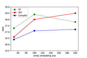
(a) Influence of entity embedding size

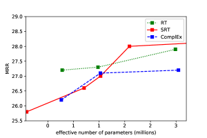
(b) Influence of model size. For RT, $d_{e}=32,52,84$ (from left to right). For SRT and ComplEx, $d_{e}=50,100,200$

Figure 3: Performance analysis on FB15K-237

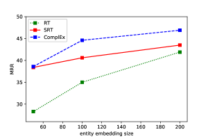
(a) Influence of entity embedding size

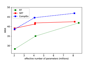
(b) Influence of model size. For all models, $d_{e}=50,100,200$ from left to right.

Figure 4: Performance analysis on WN18RR

Influence of entity embedding size.

Figures 3a) and 4a) report model performance for varying entity embedding sizes. For FB15K-237, Figure 3(a) shows that both SRT and DRT performed competitive or better than ComplEx across the entire range of $d_{e}\in\{50,100,200\}$. Sparsity constraints were helpful when $d_{e}\geq 100$: the performance of DRT decreased while SRT continued to improve on WN18RR.

Influence of effective number of parameters.

Figures 3b) and 4b) report model performance for varying model sizes, measured in terms of the effective number of parameters. The plot is a Skyline plot, i.e., we do not include model fits that are outperformed by another fit of the same model with smaller effective number of parameters.

On FB15K-237, DRT consistently outperformed ComplEx, using a smaller entity embedding size but (consequently) a larger effective relation size. Sparsity thus does not always help, and parameter sharing seemed to be beneficial. For small models, SRT performed similar to ComplEx; for larger models, SRT performed better than both ComplEx and DRT. This suggests that it is indeed possible learn sparsity patterns from the data, and that this can be beneficial. On WN18RR, ComplEx performed best as in our previous experiments. On both datasets, we found that SRT models with smaller entity embedding size $d_{e}$ usually had denser core tensors. We conjecture that this allows the SRT model to “assign” more responsibility to the core tensor with similar number of parameters.

Overall, this comparison shows decoupling $d_{e}$ and $d_{r}$ can lead to competitive models with very small entity embedding size and that sparsity does not always help when models with equal parameter sizes are compared. On the other hand, for some datasets the prescribed constraints can be very effective.

4.3 Learned Sparsity Patterns

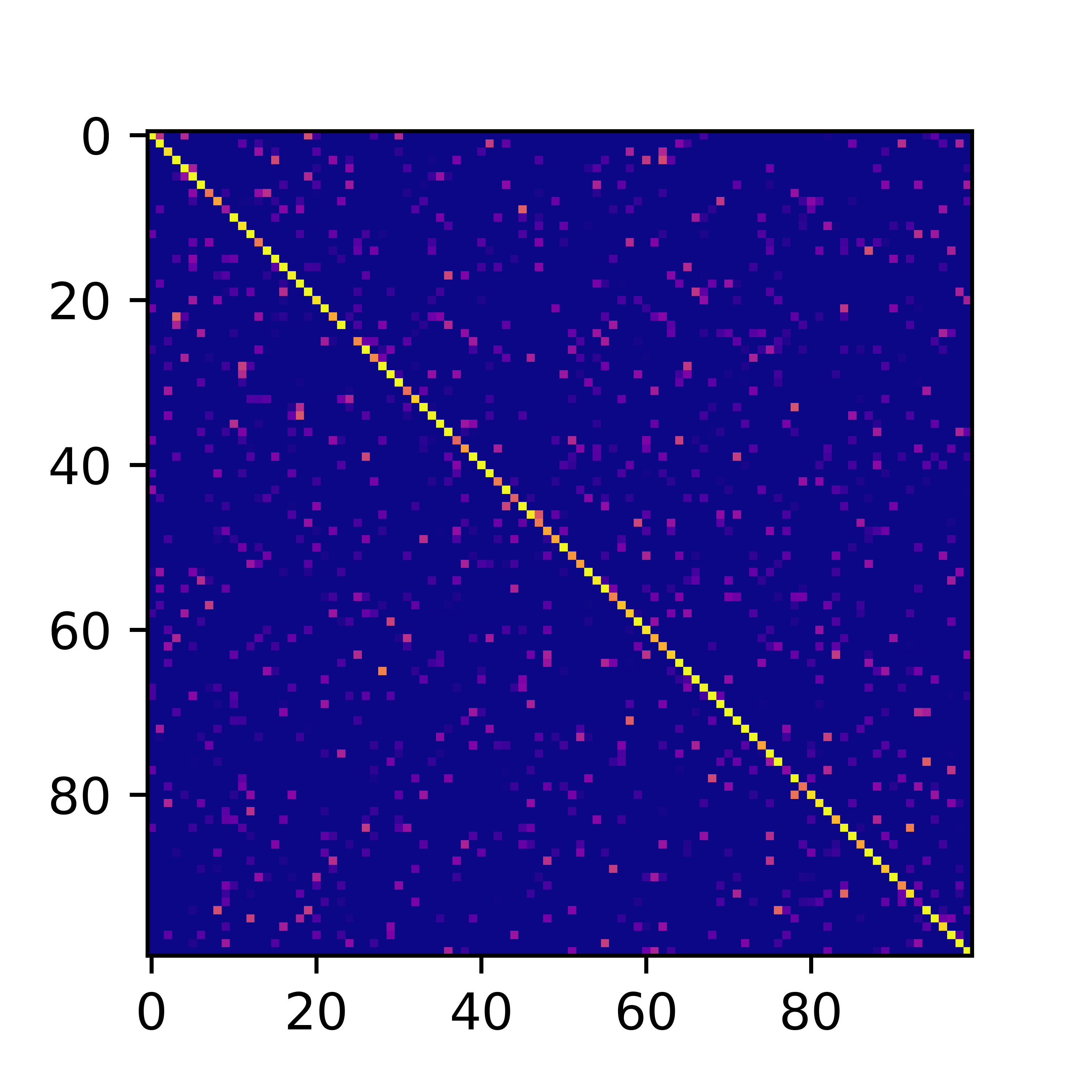
(a) win_same_award

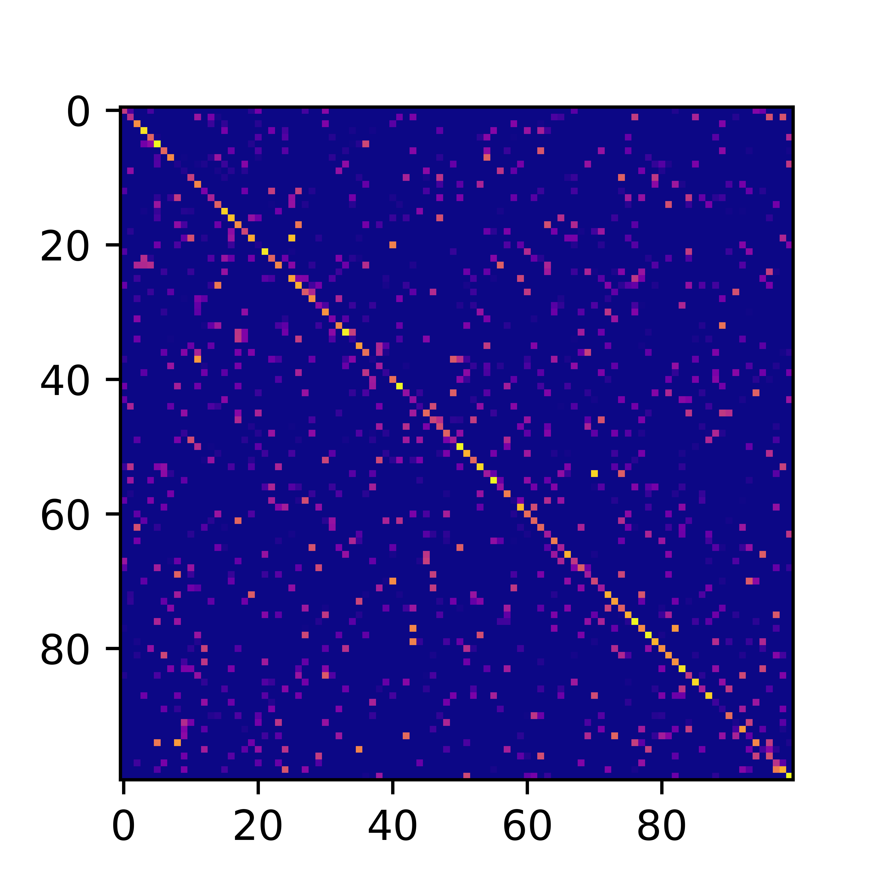
(b) location_contains

(c) type_of_union

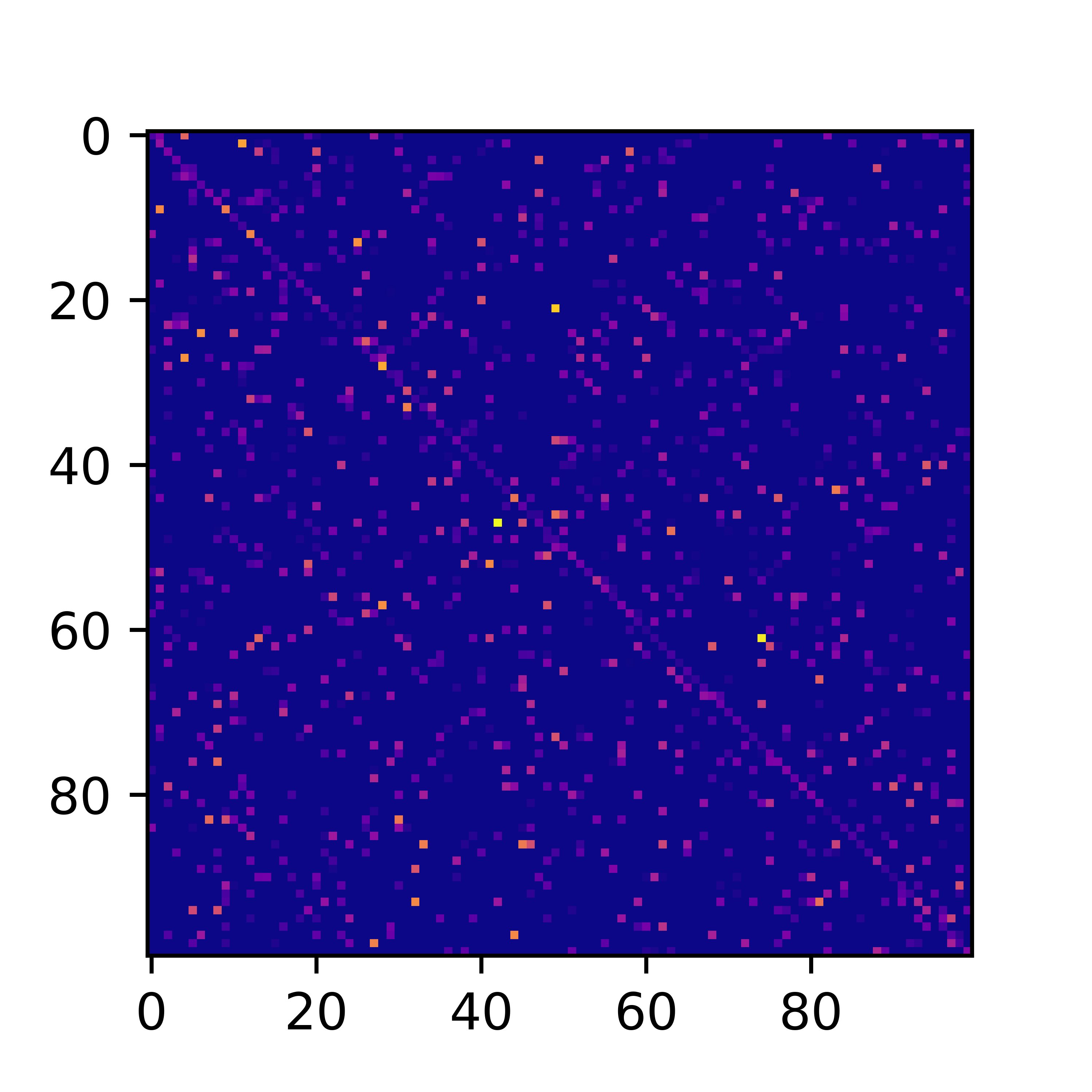
(d) gender

Figure 5: Examples of the learned sparsity patterns on the mixing matrices on FB15K-237

The sparsest SRT on FB15K-237 that we found had only $0.13\%$ of active entries in $\mathbfcal{G}$ ($d_{e}=100$, $d_{r}=100$, $d_{r}^{*}=105$), yet it performed competitive with ComplEx with the same embedding size $100$ (27.0% vs. 27.1% MRR, 45.0% vs. 45.0% HITS@$10$). Examples of the learned mixing matrices of relations (chosen from top-$30$ most frequent relations) of different semantic categories are visualized in Figure 5. Here lighter dots indicate stronger interactions. As can be seen, the diagonal entries play an important role for both the symmetric relation $win\_same\_award$ and the asymmetric relation $location\_contains$, while they are not so pronounced for the other two relations.

To get some additional insight, we compared the performance of the aforementioned SRT and ComplEx models on the top-$5$ and bottom-$5$ of the $30$ most frequent FB15K-237 relations, sorted by the sum of the absolute diagonal values of SRT’s mixing matrices. This relation-wise performance comparison shows that ComplEx had better results (29.5% vs 31.2% MRR, 44.7% vs 46.3% HITS@$10$) for relations where the learned diagonal interactions of SRT were strong (top-$5$), while SRT performed better (19.6% vs 18.7% MRR, 43.0% vs 40.7% HITS@$10$) for relations where the learned diagonal interactions were weak (bottom-$5$). The learned patterns for $win\_same\_award$ and $location\_contains$ agree to some extent with the prescribed patterns of DistMult, ComplEx, and Analogy, where the diagonal entries belong to the few active entries allowed to be active. The relation-wise performance comparison indicates that the prescribed constraint of ComplEx is not always suitable for all relations.

4.4 Computational Cost

Training SRT/DRT models is more expensive than training ComplEx, because the whole core tensor is updated in every training step. In our implementation using a single Titan X GPU, SRT/DRT with $d_{e}=200$ on FB15K-237 required around $6$ hours to train for a single configuration, while ComplEx with $d_{e}=200$ required about $1$ hour. Generally, a key advantage of models such as ComplEx is that they are more computationally-friendly.

4.5 Comparison to Previous Work

Table 3: Baseline results on FB15K-237, previous work vs. our ComplEx. The aseline results are taken from Dettmers et al. [6] for entity size $d_{e}=100$ and Lacroix et al. [13] for $d_{e}=2000$.

	Entity	Reciprocal	MRR
Model	Size	Relations
FB15K-237
ComplEx	100	Yes	24.7
ComplEx	2,000	No	35.0
Best reported	2,000	Yes	36.0
ComplEx (Ours)	100	No	27.1
ComplEx (Ours)	200	No	27.2
ComplEx (Ours)	600	No	30.0
WN18RR
ComplEx	100	Yes	44.0
ComplEx	2000	No	47.0
Best reported	2000	Yes	48.6
ComplEx (Ours)	100	No	44.6
ComplEx (Ours)	200	No	47.0
ComplEx (Ours)	600	No	49.6

We conclude this section by relating the performance of our ComplEx baseline to prior work; see Table 3. First note that Dettmers et al. [6] applied a “reciprocal relations” trick [13] during training. This trick makes the score of a triple $(i,k,j)$ becomes ambiguous. We did not use this trick in our implementations. also unclear how to use reciprocal relations in other evaluation protocols like triple classification in a principled way. In our implementation, we did not use reciprocal relations.

On both FB15K-237 and WN18RR, our ComplEx achieved better results than the one from Dettmers et al. [6] with the same entity embedding size $100$. ComplEx with $d_{e}=2000$ and reciprocal trick are the best performing models on FB15K-237. On WN18RR, our ComplEx with $d_{e}=600$ achieved the best results without using reciprocal relations. These results establish that our ComplEx implementation is a strong baseline model.

5 Conclusion

In this study we introduced the RT decomposition, and showed that existing BM are special instances of RT. In contrast to BM, the RT decomposition allows parameters sharing across different relations, and it decouples the entity and relation embedding sizes. A comparison of sparse RT (SRT) and dense RT (DRT) and ComplEx suggested that both properties can be beneficial. Dense models can achieve competitive results. While models such as ComplEx are more computationally-friendly, it is sometimes possible and even beneficial to learn better sparsity patterns.

6 Supplementary Materials

Table 4: Baseline results; previous work vs. our ComplEx

	Entity	Reciprocal	Effective	Effective	MRR	HITS
Model	Size	Relations	Relation	Number of		@1	@3	@10
			Size $d_{r}^{*}$	Parameters
FB15K-237
ComplEx [6]	100	Yes	200	1,547K	24.7	15.8	27.5	42.8
Best reported [13]	2,000	Yes	2,000	30,948K	36.0	-	-	56.0
ComplEx (Ours)	200	No	200	3,047K	27.2	17.6	30.4	46.7
ComplEx (Ours)	600	No	600	9,142K	30.0	20.7	33.2	48.3
WN18RR
ComplEx [6]	100	Yes	100	4,058K	44.0	41.0	46.0	51.0
Best reported [13]	2000	Yes	2000	81,170K	48.6	-	-	57.9
ComplEx (Ours)	200	No	200	8,114K	47.0	42.0	50.0	55.4
ComplEx (Ours)	600	No	600	24,344K	49.6	45.4	51.7	57.1

Table 5: Hyper-parameter ranges in our experiments.

	SRT	RT	ComplEx
$\lambda$	$\{5\text{e-}1,1\text{e-}1,1\text{e-}2\}$	-	-
$d_{e}$	$\{50,100,200\}$	$\{50,100,200\}$	$\{50,100,200,600\}$
$d_{R}$ (WN18RR)	$\{7,11,14\}$	$\{7,11,14\}$	-
$d_{R}$ (FB15k-237)	$\{100,160,200,237,300\}$	$\{100,160,200,237,300\}$	-
	SRT, RT, ComplEx
$\eta$	$\{0.0,0.1,0.2,0.3,0.4,$ $0.5\}$
$lr$	$\{5\text{e-}1,1\text{e-}1,5\text{e-}2,1\text{e-}2,5\text{e-}3,1\text{e-}3\}$
$\omega$	$\{10^{-4},10^{-5},10^{-6},0\}$

Detailed Base Line Results The full results for baseline comparison is summarized in Tab. 4.

Hyper-parameter Ranges

Hyper-parameter ranges for dropout $\eta$, learning rate $lr$, weight decay $\omega$, relation embedding sizes $d_{R}$, $l_{0}$ regularization parameter $\lambda$. For SRT we set the hyper-parameters for all hard-concrete variables used in $l_{0}$ regularization fixed with location mean $loc_{mean}=3.0$, location standard deviation $loc_{std}=1$, location temperature $\beta=2/3$, stretch ranges $\zeta=1.1$ and $\gamma=-0.1$. We set $\lambda=0$ for the first $25$ epochs, i.e. we initially do not include the $l_{0}$ regularization term, as it empirically improved the results.

Reciprocal Trick

The data is augmented by adding a triple $(j,k^{-1},i)$ for each $(i,k,j)$ in the data. The model then learns two relation embeddings ${\mathbf{r}}_{k}$ and ${\mathbf{r}}_{k^{-1}}$. Instead of answering questions (?, k, j) and (i,k,?), the model answers (j, $k^{-1}$, ?) and (i, k, ?). This approach empirically improved the prediction accuracy [13] in prior studies. Observe that the relation sizes are doubled and the score of a triple $(i,k,j)$ becomes ambiguous (since generally $s(i,k,j)\neq s(j,k^{-1},i)$).

References

- Abujabal et al. [2018a] Abujabal, A., Roy, R. S., Yahya, M., and Weikum, G. Never-ending learning for open-domain question answering over knowledge bases. In The Web Conference WWW, pp. 1053–1062, 2018a.
- Abujabal et al. [2018b] Abujabal, A., Roy, R. S., Yahya, M., and Weikum, G. Never-ending learning for open-domain question answering over knowledge bases. In The Web Conference WWW, pp. 1053–1062, 2018b.
- Bast et al. [2016] Bast, H., Buchhold, B., and Haussmann, E. Semantic search on text and knowledge bases. Foundations and Trends in Information Retrieval, 10(2-3):119–271, 2016.
- Bordes et al. [2013] Bordes, A., Usunier, N., García-Durán, A., Weston, J., and Yakhnenko, O. Translating embeddings for modeling multi-relational data. In Advances in Neural Information Processing Systems, NIPS, pp. 2787–2795, 2013.
- Carroll & Chang [1970] Carroll, J. D. and Chang, J.-J. Analysis of individual differences in multidimensional scaling via an n-way generalization of “eckart-young” decomposition. Psychometrika, 35(3):283–319, Sep 1970.
- Dettmers et al. [2018] Dettmers, T., Minervini, P., Stenetorp, P., and Riedel, S. Convolutional 2d knowledge graph embeddings. In Association for the Advancement of Artificial Intelligence, AAAI, 2018.
- Duchi et al. [2011] Duchi, J. C., Hazan, E., and Singer, Y. Adaptive subgradient methods for online learning and stochastic optimization. Journal of Machine Learning Research, 12:2121–2159, 2011.
- Galarraga et al. [2013] Galarraga, L. A., Teflioudi, C., Hose, K., and Suchanek, F. M. Amie: association rule mining under incomplete evidence in ontological knowledge bases. In The Web Conference WWW, pp. 413–422, 2013.
- Guo et al. [2018] Guo, S., Wang, Q., Wang, L., Wang, B., and Guo, L. Knowledge graph embedding with iterative guidance from soft rules. In Association for the Advancement of Artificial Intelligence, AAAI, pp. 4816–4823, 2018.
- Hayashi & Shimbo [2017] Hayashi, K. and Shimbo, M. On the equivalence of holographic and complex embeddings for link prediction. In ACL (2), pp. 554–559, 2017.
- Kazemi & Poole [2018] Kazemi, S. M. and Poole, D. Simple embedding for link prediction in knowledge graphs. In Advances in Neural Information Processing Systems NeurIPS, pp. 4289–4300, 2018.
- Kolda & Bader [2009] Kolda, T. G. and Bader, B. W. Tensor decompositions and applications. SIAM Review, 51(3):455–500, 2009.
- Lacroix et al. [2018] Lacroix, T., Usunier, N., and Obozinski, G. Canonical tensor decomposition for knowledge base completion. In International Conference on Machine Learning, ICML, pp. 2869–2878, 2018.
- Lao et al. [2011] Lao, N., Mitchell, T., and Cohen, W. W. Random walk inference and learning in a large scale knowledge base. In Empirical Methods in Natural Language Processing, EMNLP, 2011.
- Lehmann et al. [2015] Lehmann, J., Isele, R., Jakob, M., Jentzsch, A., Kontokostas, D., Mendes, P. N., Hellmann, S., Morsey, M., van Kleef, P., Auer, S., and Bizer, C. Dbpedia - A large-scale, multilingual knowledge base extracted from wikipedia. Semantic Web, 6(2):167–195, 2015.
- Liu et al. [2017a] Liu, H., Wu, Y., and Yang, Y. Analogical inference for multi-relational embeddings. In International Conference on Machine Learning, ICML, pp. 2168–2178, 2017a.
- Liu et al. [2017b] Liu, H., Wu, Y., and Yang, Y. Analogical inference for multi-relational embeddings. In International Conference on Machine Learning, ICML, volume 70, pp. 2168–2178, 2017b.
- Louizos et al. [2017] Louizos, C., Welling, M., and Kingma, D. P. Learning sparse neural networks through l regularization. CoRR, 2017.
- Maddison et al. [2017] Maddison, C. J., Mnih, A., and Teh, Y. W. The concrete distribution: A continuous relaxation of discrete random variables. International Conference on Learning Representations ICLR, 2017.
- Meilicke et al. [2018] Meilicke, C., Fink, M., Wang, Y., Ruffinelli, D., Gemulla, R., and Stuckenschmidt, H. Fine-grained evaluation of rule- and embedding-based systems for knowledge graph completion. In International Semantic Web Conference, ISWC, 2018.
- Nickel et al. [2011] Nickel, M., Tresp, V., and Kriegel, H. A three-way model for collective learning on multi-relational data. In International Conference on Machine Learning, ICML, pp. 809–816, 2011.
- Nickel et al. [2016a] Nickel, M., Murphy, K., Tresp, V., and Gabrilovich, E. A review of relational machine learning for knowledge graphs. IEEE Computer Society, 104(1):11–33, 2016a.
- Nickel et al. [2016b] Nickel, M., Rosasco, L., and Poggio, T. A. Holographic embeddings of knowledge graphs. In Association for the Advancement of Artificial Intelligence, AAAI, pp. 1955–1961, 2016b.
- Rebele et al. [2016] Rebele, T., Suchanek, F. M., Hoffart, J., Biega, J., Kuzey, E., and Weikum, G. YAGO: A multilingual knowledge base from Wikipedia, Wordnet, and Geonames. In ISWC, LNCS, pp. 9982:177–185, 2016.
- Socher et al. [2013] Socher, R., Chen, D., Manning, C. D., and Ng, A. Y. Reasoning with neural tensor networks for knowledge base completion. In Advances in Neural Information Processing Systems, NIPS, pp. 926–934, 2013.
- Toutanova et al. [2015] Toutanova, K., Chen, D., Pantel, P., Poon, H., Choudhury, P., and Gamon, M. Representing text for joint embedding of text and knowledge bases. In Empirical Methods in Natural Language Processing, EMNLP, pp. 1499–1509, 2015.
- Trouillon & Nickel [2017] Trouillon, T. and Nickel, M. Complex and holographic embeddings of knowledge graphs: A comparison. CoRR, abs/1707.01475, 2017.
- Trouillon et al. [2016] Trouillon, T., Welbl, J., Riedel, S., Gaussier, É., and Bouchard, G. Complex embeddings for simple link prediction. In International Conference on Machine Learning, ICML, pp. 2071–2080, 2016.
- Tucker [1966] Tucker, L. R. Some mathematical notes on three-mode factor analysis. Psychometrika, 31(3):279–311, Sep 1966.
- Wang et al. [2018a] Wang, H., Zhang, F., Wang, J., Zhao, M., Li, W., Xie, X., and Guo, M. Ripplenet: Propagating user preferences on the knowledge graph for recommender systems. In International Conference on Information and Knowledge Management CIKM, pp. 417–426, 2018a.
- Wang et al. [2018b] Wang, Y., Gemulla, R., and Li, H. On multi-relational link prediction with bilinear models. In Association for the Advancement of Artificial Intelligence, AAAI, 2018b.
- Wang et al. [2014] Wang, Z., Zhang, J., Feng, J., and Chen, Z. Knowledge graph embedding by translating on hyperplanes. In Association for the Advancement of Artificial Intelligence, AAAI, pp. 1112–1119, 2014.
- Yang et al. [2014] Yang, B., Yih, W., He, X., Gao, J., and Deng, L. Embedding entities and relations for learning and inference in knowledge bases. CoRR, abs/1412.6575, 2014.
- Zhang et al. [2016] Zhang, F., Yuan, N. J., Lian, D., Xie, X., and Ma, W. Collaborative knowledge base embedding for recommender systems. In PInternational Conference on Knowledge Discovery and Data Mining SIGKDD, pp. 353–362, 2016.