Jost function based on the Hartree-Fock-Bogoliubov formalism

Abstract

We formulate the Jost function formalism based on the Hartree-Fock-Bogoliubov (HFB) theory which has been used to represent the nature of the superfluidity of nucleus. The Jost function based on the HFB can give the analytic representation of the S-matrix for the nucleon elastic scattering targeting on the open-shell nucleus taking into account the pairing effect. By adopting the Woods-Saxon potential, we show the numerical results of S-matrix poles and their trajectories with varying the pairing strength in two cases of Fermi energies: $\lambda=-8.0$ and $-1.0$ MeV. The total cross sections in each cases for neutron elastic scattering are also analyzed, and we confirmed some staggering shapes or sharp resonances originated from the effect of pairing can be seen in the cross section.

I Introduction

The coefficient functions of the regular solution of the Schrödinger equation for scattering introduced by Jost jost has been known as the Jost function. They have been used to identify the S-matrix poles for the bound states and resonances of the system on the complex energy/momentum plane.

The S-matrix poles represent the bound states and the resonance energy and width. The analysis of S-matrix poles has been performed on the scattering data to investigate the properties of the potential of the target. An interesting study is to investigate the trajectories of the S-matrix poles on the complex energy/momentum plane shown as a function of the potential depth Hussein . It is also possible to analyze the channel coupling effect in terms of the S-matrix poles on the Riemann sheets defined for each channels Rod ; Hans .

The optical potential is indispensable to a reliable extraction of nuclear structure information from experimental data of various direct nuclear reactions such as inelastic scattering and transfer reactions. The global optical potentials(GOP) have been investigated for long time watson ; Bec ; Nada ; Var ; Hama ; Cooper ; Koning ; Kunieda ; Han1 ; Perey ; Dae ; Boj ; An ; Han2 , and succeeded to reproduce the experimental cross section with high accuracy. The GOP is given by the complex function, the imaginary part gives the absorption of the target nucleus for the current of the incident beam. The existence of the imaginary part of the GOP has been justified qualitatively by the Feshbach projection theoryfeshbach .

Recently, the self-consistent particle-vibration coupling (PVC) method has been applied to the nucleon-nucleus ($NA$) scattering mizuyama ; mizuyama2 ; branchon ; hao . The experimental data for neutron elastic scattering on ¹⁶O mizuyama , proton inelastic scattering on ²⁴O mizuyama2 , neutron elastic scattering on ⁴⁰Ca, its analyzing power branchon , and neutron elastic scattering on ¹⁶O and ²⁰⁸Pb mizuyama were successfully reproduced. In the PVC framework, the microscopic optical potential is given as the non-local complex potential which gives the proper absorption for the reproduction of the experimental cross section. These results are consistent with the Feshbach projection theory, and give the quantitative justification for the existence of the imaginary part of the GOP.

It is well known that there are many sharp peaks are observed at low-energy in the total and elastic cross section of the $NA$-scattering. Such resonances have been analyzed by using the R-matrix theory rmatrix , The R-matrix theory is a phenomenological framework in which reactions of neutrons, charged particles + nuclei are described quantum mechanically based on boundary conditions for various channels and the scattering matrix (S-matrix) is acquired from measurement data of cross section. Obtained resonance parameters have been published as the nuclear data jendl ; jeff ; endf and used for many applications (Nuclear engineering, radiotherapy, etc.) because nuclear resonances are very useful characteristic for the applications.

It was also shown that the sharp resonances appeared in the neutron elastic scattering can be partially reproduced due to the coupling between the induced neutron and the giant resonance of the target nucleus mizuyama . This is also consistent with the Feshbach theory which justified the R-matrix theory and its resonance formula. Very recently, the multichannel algebraic scattering method (MCAS) which is based on the phenomenological vibrational model has been applied to study the bound and resonance properties of the ¹⁷O and ¹⁷F nuclei below and above the nucleon -core threshold. The narrow resonances of the experimental data could be reproduced successfully amos .

The results of these recent progress and attempts at low energy $NA$ scattering may indicate the possibility of a new phenomenological model based on the microscopic theory of nuclear structure and reaction. However, the pairing correlation has not been discussed in the direction of these recent progress.

The importance of the pairing correlation has been discussed mainly in the nuclear structure. The pairing correlation in nuclei is very important to explain the fundamental properties of nuclei, such as the magic number, the separation energy and the quadrupole 1st excited state of nucleus, and so on. In the last decades, the investigation of the pairing effect on nuclear structure has been held based on the microscopic theoretical framework, such as the Hartree-Fock-Bardeen-Cooper-Schrieffer (HF+BCS) hfbcs2017 , the Hartree-Fock-Bogoliubov (HFB) hfb2010 , the Highly Truncated Diagonalization Approach (HTDA) htda2002 ; htda2012 and the Quasiparticle Random Phase Approximation (QRPA) hfb1 ; qrpa1 ; qrpaC ; qrpaT . Di-neutron correlation resulting from the coherent overlap of the continuum states due to the pair correlation at both ground state and the low-lying excitation of the neutron drip line nuclei has been discussed qrpa1 . Also the quasiparticle resonances of the neutron drip-line nuclei have been investigated within the framework of HFBhamamoto ; hamamoto2 ; zhang ; kobayashi ; grasso ; fayans2 ; michel ; Pei ; zhang2 ; oba ; zhang3 ; Sand ; betan ; sand2 . The experimental cross section of d(⁹Li,¹⁰Li)p was also analyzed from the point of the pair resonance based on the HFB formalism orrigo2 .

Nevertheless, the role of the pairing correlation for the reaction is not clear yet. The pairing correlation may have the important role for the reaction and the channel coupling in which two neutron transfer channel is relevant ptrf . In order clarify the role of the pairing in the reaction, it may be necessary to investigate the pairing effect in terms of the S-matrix poles. The aim of this work is to derive the Jost function formalism based on the HFB formalism in order to discuss the pairing effect on $NA$-scattering in terms of the S-matrix poles.

This paper is organized as follows. We introduce the definition of the complex quasiparticle energy and momentum basing on the HFB equation in Sec.II. We show the derivation of the Jost function based on the HFB equation, the definition of the S-matrix and its unitarity in Sec.III. In Sec.IV, we demonstrate the numerical results adopting the Woods-Saxon potential. The poles of the S-matrix and their trajectories with varying the paring strength are shown. The appearance of the quasiparticle resonances on the total cross section of the neutron elastic scattering cross section is also discussed.

II Definitions of complex energy & momentum planes

The Hartree-Fock-Bogoliubov(HFB) equation can be represented as

$$\left[\left(\frac{\partial^{2}}{\partial r^{2}}-\frac{l(l+1)}{r^{2}}\right)\mbox{\boldmath$1$}-\widehat{S}_{z}\mathcal{U}_{lj}(r)\right]\phi_{lj}(r;E)$$

$$\hskip 56.9055pt=-\begin{pmatrix}k_{1}^{2}(E)&0\\ 0&k_{2}^{2}(E)\end{pmatrix}\phi_{lj}(r;E),$$ (1)

$$\mathcal{U}_{lj}(r)=\frac{2m}{\hbar^{2}}\begin{pmatrix}U_{lj}(r)&\Delta(r)\\ \Delta(r)&-U_{lj}(r)\end{pmatrix},$$ (2)

$$\phi_{lj}(r;E)=\begin{pmatrix}\varphi_{1,lj}(r;E)\\ \varphi_{2,lj}(r;E)\end{pmatrix},$$ (3)

where $E$ is the quasi-particle energy defined as positive value, $U_{lj}(r)$ and $\Delta(r)$ are the (Hartree-Fock) mean-field potential and the pairing potential, respectively. Where $1$ is the unit matrix, and $\widehat{S}_{z}$ is the third component of the Pauli matrix given by

$$\widehat{S}_{z}=\begin{pmatrix}1&0\\ 0&-1\end{pmatrix},$$ (4)

$k_{1}(E)$ and $k_{2}(E)$ are momentum defined by

$$k_{1}(E) \equiv \sqrt{\frac{2m}{\hbar^{2}}(\lambda+E)},$$ (5)

$$k_{2}(E) \equiv \sqrt{\frac{2m}{\hbar^{2}}(\lambda-E)},$$ (6)

for upper and lower components of quasiparticle wave functions of HFB equation, respectively. $\lambda$ is the Fermi energy defined as negative value in the case of the bound target. On the complex-$E$ plane, $\lambda\pm E$ can be represented as

$$\lambda+E = |\lambda+E|e^{i\theta_{1}(E)},$$ (7)

$$\lambda-E = |E-\lambda|e^{i(\theta_{2}(E)+\pi)},$$ (8)

where $\theta_{1}(E)$ and $\theta_{2}(E)$ are angles defined on the complex-$E$ plane as shown in Figs.1 and 2. The definition range of angle is $0\leq\theta_{1,2}(E)\leq 2\pi$.

Inserting Eqs.(7) and (8) into Eqs.(5) and (6), respectively, we can obtain

$$k_{1}(E) = |k_{1}(E)|e^{i\theta_{1}(E)/2}e^{in\pi}\hskip 14.22636pt(n=0,1),$$ (9)

$$|k_{1}(E)| \equiv \sqrt{\frac{2m}{\hbar^{2}}|\lambda+E|},$$ (10)

$$k_{2}(E) = i|k_{2}(E)|e^{i\theta_{2}(E)/2}e^{in\pi}\hskip 14.22636pt(n=0,1),$$ (11)

$$|k_{2}(E)| \equiv \sqrt{\frac{2m}{\hbar^{2}}|E-\lambda|},,$$ (12)

the factor $e^{in\pi}(n=0,1)$ is due to the phase ambiguity which shows that the complex energy plane consists of two Riemann sheets. By using $n(=0,1)$, let us define the $(n+1)$th Riemann sheet, $E_{n+1}$. We chose the energy dependent angles $\theta_{1,2}(E)$ have the relation as

$$\theta_{1,2}(E)+2n\pi$$

$$\to\theta_{1,2}(E_{2})=\theta_{1,2}(E_{1})+2\pi,$$ (13)

so that the first Riemann sheet has the scattering and bound states, and the second Riemann sheet has the resonance states. Inserting this condition into Eqs.(9) and (11), it is easy to find that $k_{1,2}(E)$ have the relation

$$k_{1,2}(E_{2})=-k_{1,2}(E_{1}).$$ (14)

and the upper/lower half of the complex momentum-$k_{1,2}$ correspond to the first/second Riemann sheets respectively. The branch cut is set for each $k_{1}(E)$ and $k_{2}(E)$ as shown in Fig.1, Fig.2, Fig.3 and Fig.4.

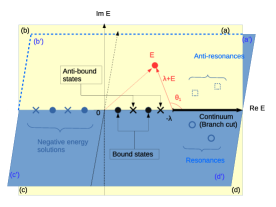
Figure 1: (Color online) Complex quasiparticle energy planes with S-matrix poles corresponding bound states, anti-bound states, resonances and anti-resonances. The angle $\theta_{1}$ which is used in Eq.(9) is also shown. The branch cut corresponding Re $k_{1}$ line of scattering states is shown by the black solid arrow on the real axis above $-\lambda$. Four quadrants of the first Riemann sheet (a)-(d) correspond to four areas of the upper half plane of $k_{1}$ shown as (a)-(d) in Fig.2. Four quadrants of the second Riemann sheet (a’)-(d’) correspond to four areas of the lower half plane of $k_{1}$ shown as (a’)-(d’) in Fig.2.

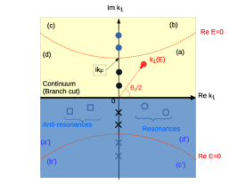
Figure 2: (Color online) Complex $k_{1}$-momentum plane corresponding the complex energy plane shown in Fig.1. Corresponding states are shown by using the same colors and symbols. The black solid arrow on Re $k_{1}$ indicates the scattering states corresponding the branch cut on the complex energy plane. The upper/lower half plane correspond to the first/second Riemann sheets of the complex energy. The hyperbola shown by dotted red curve represent the $k_{1}$-momentum with Re $E=0$. $k_{F}$ is defined by $k_{F}=\sqrt{\frac{2m|\lambda|}{\hbar^{2}}}$.

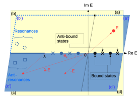
Figure 3: (Color online) Same figure with Fig.1 but with branch cut defined by $k_{2}$-momentum.

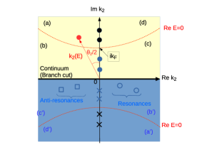
Figure 4: (Color online) Same figure with Fig.2 but relevant to $k_{2}$-momentum.

III Jost function based on the HFB formalism

In general, the double differential equation such as the Schrödinger equation has the regular and irregular solutions. The regular solution can be represented by the linear combination of the linear independent irregular solutions. If the irregular solutions satisfy the out-going (or in-coming) boundary condition, the Jost function is defined as the coefficients for the linear combination jost .

In this section, we derive the Jost function basing on the HFB formalism. The HFB equation has two independent solutions for regular solutions and irregular solutions, respectively.

Applying the Green’s theorem, it is possible to describe the regular and irregular solution in the integral equation form. The Green’s theorem for the HFB equation is given by

$$\left[\chi_{l}^{\mathrm{T}}(r;E)\widehat{S}_{z}\frac{\partial\phi_{lj}(r;E)}{\partial r}-\frac{\partial\chi_{l}^{\mathrm{T}}(r;E)}{\partial r}\widehat{S}_{z}\phi_{lj}(r;E)\right]_{r=a}^{r=b}$$

$$=\frac{2m}{\hbar^{2}}\int_{a}^{b}dr^{\prime}\chi_{l}^{\mathrm{T}}(r^{\prime};E)\mathcal{U}_{lj}(r^{\prime})\phi_{lj}(r^{\prime};E),$$ (15)

where $\chi_{l}^{\mathrm{T}}(r;E)$ is the free particle wave function which satisfies

$$\left(\frac{\partial^{2}}{\partial r^{2}}-\frac{l(l+1)}{r^{2}}\right)\chi_{l}(r;E)=-\begin{pmatrix}k_{1}^{2}(E)&0\\ 0&k_{2}^{2}(E)\end{pmatrix}\chi_{l}(r;E).$$

(16)

In general, the second derivative equation has two independent solutions; $\phi_{lj}^{(rs)}(r;E)$ which is regular at the origin $r=0$ and $\phi_{lj}^{(\pm s)}(r;E)$ satisfies the out-going boundary condition at the asymptotic limit $r\to\infty$. The HFB equation has two independent solutions for each $\phi_{lj}^{(rs)}(r;E)$ and $\phi_{lj}^{(\pm s)}(r;E)$ which are described with the subscription $s=1,2$ as introduced in matsuo .

By supposing

$$\lim_{r\to 0}\left[\chi_{l}^{(\pm s)\mathrm{T}}(r;E)\widehat{S}_{z}\frac{\partial\phi_{l}^{(rs^{\prime})}(r;E)}{\partial r}\right.$$

$$\hskip 85.35826pt\left.-\frac{\partial\chi_{l}^{(\pm s)\mathrm{T}}(r;E)}{\partial r}\widehat{S}_{z}\phi_{l}^{(rs^{\prime})}(r;E)\right]$$

$$=\mp\frac{i}{k_{s}(E)}\langle s|\widehat{S}_{z}|s^{\prime}\rangle,$$ (17)

with $\chi_{l}^{(\pm s)\mathrm{T}}(r;E)$ defined by the spherical Hankel function as

$$\chi_{l}^{(\pm 1)}(r;E) = \begin{pmatrix}rh^{(\pm)}_{l}(k_{1}(E)r)\\ 0\end{pmatrix},$$ (18)

$$\chi_{l}^{(\pm 2)}(r;E) = \begin{pmatrix},0\\ rh^{(\pm)}_{l}(k_{2}(E)r)\end{pmatrix}$$ (19)

and taking $a\to 0$ and $b\to r$ for Eq.(15), we can derive the integral form of $\phi_{lj}^{(rs)}(r;E)$ as

$$\phi_{lj}^{(rs)}(r;E) = \chi_{l}^{(rs)}(r;E)$$

$$+\int_{0}^{\infty}dr^{\prime}\mathcal{G}_{FR,l}(rr^{\prime};E)\mathcal{U}_{lj}(r^{\prime})\phi_{lj}^{(rs)}(r^{\prime};E),$$

(20)

$$\chi_{l}^{(rs)}(r;E) = \frac{1}{2}\left[\chi_{l}^{(+s)}(r;E)+\chi_{l}^{(-s)}(r;E)\right],$$ (21)

with the Green’s function defined by

$$\mathcal{G}_{FR,l}(rr^{\prime};E)$$

$$=-\frac{2m}{\hbar^{2}}\sum_{s=1,2}\frac{k_{s}(E)}{2i}\theta(r-r^{\prime})\widehat{S}_{z}$$

$$\times\left[\chi_{l}^{(-s)}(r;E)\chi_{l}^{(+s)\mathrm{T}}(r^{\prime};E)-\chi_{l}^{(+s)}(r;E)\chi_{l}^{(-s)\mathrm{T}}(r^{\prime};E)\right]$$

(22)

$$=\begin{pmatrix}g_{FR,l}(rr^{\prime};k_{1}(E))&0\\ 0&-g_{FR,l}(rr^{\prime};k_{2}(E))\end{pmatrix},$$ (23)

where

$$g_{FR,l}(rr^{\prime};k)$$

$$\equiv-\frac{2m}{\hbar^{2}}\frac{k}{2i}\theta(r-r^{\prime})rr^{\prime}$$

$$\times\left[h^{(-)}_{l}(kr)h^{(+)}_{l}(kr^{\prime})-h^{(-)}_{l}(kr^{\prime})h^{(+)}_{l}(kr)\right],$$ (24)

Note that Eq.(17) is the so-called Robin boundary condition robin at the origin. The Robin boundary condition is the combination of the Dirichlet and Neumann boundary conditions.

The asymptotic boundary condition of $\phi_{lj}^{(\pm s)}(r;E)$ at the limit $r\to\infty$ is given by

$$\lim_{r\to\infty}\phi_{lj}^{(\pm 1)}(r;E) \to \begin{pmatrix}rh^{(\pm)}_{l}(k_{1}(E)r)\\ 0\end{pmatrix},$$ (25)

$$\lim_{r\to\infty}\phi_{lj}^{(\pm 2)}(r;E) \to \begin{pmatrix}0\\ rh^{(\pm)}_{l}(k_{2}(E)r)\end{pmatrix}.$$ (26)

Taking $a\to r$ and $b\to\infty$ for Eq.(15) with these boundary conditions, we can obtain the integral form of $\phi_{lj}^{(\pm s)}(r;E)$ as

$$\phi_{lj}^{(\pm s)}(r;E)$$

$$=\chi_{l}^{(\pm s)}(r;E)+\int_{0}^{\infty}dr^{\prime}\mathcal{G}_{FL,l}(rr^{\prime};E)\mathcal{U}_{lj}(r^{\prime})\phi_{lj}^{(\pm s)}(r^{\prime};E)$$

, (27)

with the Green’s function defined by

$$\mathcal{G}_{FL,l}(rr^{\prime};E)$$

$$=\frac{2m}{\hbar^{2}}\sum_{s=1,2}\frac{k_{s}(E)}{2i}\theta(r^{\prime}-r)\widehat{S}_{z}$$

$$\times\left[\chi_{l}^{(-s)}(r;E)\chi_{l}^{(+s)\mathrm{T}}(r^{\prime};E)-\chi_{l}^{(+s)}(r;E)\chi_{l}^{(-s)\mathrm{T}}(r^{\prime};E)\right]$$

(28)

$$=\begin{pmatrix}g_{FL,l}(rr^{\prime};k_{1}(E))&0\\ 0&-g_{FL,l}(rr^{\prime};k_{2}(E))\end{pmatrix},$$ (29)

where

$$g_{FL,l}(rr^{\prime};k)$$

$$\equiv\frac{2m}{\hbar^{2}}\frac{k}{2i}rr^{\prime}\theta(r^{\prime}-r)$$

$$\times\left[h^{(-)}_{l}(kr)h^{(+)}_{l}(kr^{\prime})-h^{(-)}_{l}(kr^{\prime})h^{(+)}_{l}(kr)\right]$$ (30)

. It should be noted that we used the value of Wronskian for the spherical Hankel function given by

$$W(rh^{(+)}_{l}(kr),rh^{(-)}_{l}(kr))=-\frac{2i}{k},$$ (31)

in order to derive Eq.(27).

By notifying the relation between $\mathcal{G}_{FR,l}$ and $\mathcal{G}_{FL,l}$ given by

$$\mathcal{G}_{FR,l}(rr^{\prime};E)=\mathcal{G}_{FL,l}(rr^{\prime};E)$$

$$-\frac{2m}{\hbar^{2}}\sum_{s=1,2}\frac{k_{s}(E)}{2i}\widehat{S}_{z}$$

$$\times\left[\chi_{l}^{(-s)}(r;E)\chi_{l}^{(+s)\mathrm{T}}(r^{\prime};E)-\chi_{l}^{(+s)}(r;E)\chi_{l}^{(-s)\mathrm{T}}(r^{\prime};E)\right],$$

we can easily find the relation between $\phi_{lj}^{(rs)}$ and $\phi_{lj}^{(\pm s)}$ given by

$$\phi_{lj}^{(rs)}(r;E) = \frac{1}{2}\sum_{s^{\prime}=1,2}\left[\left(\mathcal{J}_{lj}^{(+)}(E)\right)_{ss^{\prime}}\phi_{lj}^{(-s^{\prime})}(r;E)\right.$$ (33)

$$\left.+\left(\mathcal{J}_{lj}^{(-)}(E)\right)_{ss^{\prime}}\phi_{lj}^{(+s^{\prime})}(r;E)\right],$$

where $\left(\mathcal{J}_{lj}^{(\pm)}(E)\right)_{ss^{\prime}}$ is the Jost function defined by

$$\left(\mathcal{J}_{lj}^{(\pm)}(E)\right)_{ss^{\prime}}\equiv\delta_{ss^{\prime}}$$

$$\mp\langle s^{\prime}|\widehat{S}_{z}|s^{\prime}\rangle\frac{2m}{\hbar^{2}}\frac{k_{s^{\prime}}(E)}{i}\int_{0}^{\infty}dr\chi_{l}^{(\pm s^{\prime})\mathrm{T}}(r;E)\mathcal{U}_{lj}(r)\phi_{lj}^{(rs)}(r;E).$$

(34)

This Jost function can be also expressed as

$$\left(\mathcal{J}_{lj}^{(\pm)}(E)\right)_{ss^{\prime}}$$

$$=\delta_{ss^{\prime}}$$

$$\mp\langle s^{\prime}|\widehat{S}_{z}|s^{\prime}\rangle\frac{k_{s^{\prime}}(E)}{i}\frac{2m}{\hbar^{2}}\int_{0}^{\infty}dr\chi_{l}^{(rs)\mathrm{T}}(r;E)\mathcal{U}_{lj}(r)\phi_{lj}^{(\pm s^{\prime})}(r;E)$$

(35)

$$=\pm\langle s^{\prime}|\widehat{S}_{z}|s^{\prime}\rangle\frac{k_{s^{\prime}}(E)}{i}\frac{2m}{\hbar^{2}}w_{lj}^{s,\pm s^{\prime}}(E),$$ (36)

where $w_{lj}^{s,\pm s^{\prime}}(E)$ is the Wronskian for the HFB solutions defined by

$$w_{lj}^{s,\pm s^{\prime}}(E)\equiv\frac{\hbar^{2}}{2m}\left[\frac{\partial\phi_{l}^{(\pm s^{\prime})\mathrm{T}}(r;E)}{\partial r}\widehat{S}_{z}\phi_{l}^{(rs)}(r;E)\right.$$

$$\hskip 56.9055pt-\left.\phi_{l}^{(\pm s^{\prime})\mathrm{T}}(r;E)\widehat{S}_{z}\frac{\partial\phi_{l}^{(rs)}(r;E)}{\partial r}\right],$$ (37)

as introduced in matsuo ; fayans ; belyaev .

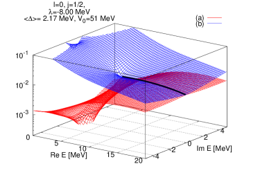
Figure 5: (Color online) The absolute value surface of the denominator ((a) red colored surface) and the denominator ((b) blue colored surface) of the S-matrix Eq.(44) for $s_{1/2}$. The black solid curve is a curve where the red and blue surfaces ((a) and (b)) are touched each other.

Note that the off-diagonal components of the Jost function becomes $\left(\mathcal{J}_{lj}^{(\pm)}(E)\right)_{12}=\left(\mathcal{J}_{lj}^{(\pm)}(E)\right)_{21}=0$ at the no pairing limit $\langle\Delta\rangle\to 0$.

The asymptotic behaviour at $r\to\infty$ of Eq.(33) is given by

$$\lim_{r\to\infty}\phi_{lj}^{(rs)}(r;E)$$

$$\sim\frac{i^{l+1}}{2k_{1}(E)}\left[\left(\mathcal{J}_{lj}^{(+)}(E)\right)_{s1}\begin{pmatrix}e^{-ik_{1}(E)r}\\ 0\end{pmatrix}\right.$$

$$\hskip 42.67912pt\left.+(-)^{l+1}\left(\mathcal{J}_{lj}^{(-)}(E)\right)_{s1}\begin{pmatrix}e^{+ik_{1}(E)r}\\ 0\end{pmatrix}\right]$$

$$+\frac{i^{l+1}}{2k_{2}(E)}\left[\left(\mathcal{J}_{lj}^{(+)}(E)\right)_{s2}\begin{pmatrix}0\\ e^{-ik_{2}(E)r}\end{pmatrix}\right.$$

$$\hskip 42.67912pt\left.+(-)^{l+1}\left(\mathcal{J}_{lj}^{(-)}(E)\right)_{s2}\begin{pmatrix}0\\ e^{+ik_{2}(E)r}\end{pmatrix}\right].$$ (38)

If the the complex quasiparticle energy $E$ belongs to the 1st Riemann sheet ($E=E_{1}$), the complex momentum $k_{1}$ and $k_{2}$ belong to the upper-half plane of each momentum planes as explained in Sec.II. The condition for the bound states are, therefore, given by

$$\left(\mathcal{J}_{lj}^{(+)}(E_{1})\right)_{s1}=\left(\mathcal{J}_{lj}^{(+)}(E_{1})\right)_{s2}=0,$$ (39)

or

$$\det\left(\mathcal{J}_{lj}^{(+)}(E_{1})\right)=0.$$ (40)

When $\det\left(\mathcal{J}_{lj}^{(+)}(E)\right)\neq 0$, the scattering wave function $\psi_{lj}^{(+)}(r;E)$ can be defined using the inverse of the Jost function $\left(\mathcal{J}_{lj}^{(+)}(E)\right)^{-1}$ as

$$\psi_{lj}^{(+)}(r;E)\equiv\sum_{s=1,2}\left(\mathcal{J}_{lj}^{(+)}(E)\right)^{-1}_{1s}\phi_{lj}^{(rs)}(r;E).$$ (41)

since the upper component of the HFB solution corresponding to particle states at no pairing limit ($\Delta(r)\to 0$) in the positive energy region (Re $E>0$).

The asymptotic behaviour of $\psi_{lj}^{(+)}(r;E)$ is given by

$$\lim_{r\to\infty}\psi_{lj}^{(+)}(r;E)$$

$$\sim\frac{i^{l+1}}{2k_{1}(E)}\left[\begin{pmatrix}e^{-ik_{1}(E)r}\\ 0\end{pmatrix}\right.$$

$$\hskip 71.13188pt\left.+(-)^{l+1}S^{11}_{lj}(E)\begin{pmatrix}e^{+ik_{1}(E)r}\\ 0\end{pmatrix}\right]$$

$$\hskip 14.22636pt+\frac{(-i)^{l+1}}{2k_{2}(E)}S^{12}_{lj}(E)\begin{pmatrix}0\\ e^{+ik_{2}(E)r}\end{pmatrix},$$ (42)

where

$$S^{ss^{\prime}}_{lj}(E)\equiv\sum_{s^{\prime\prime}=1,2}\left(\mathcal{J}_{lj}^{(+)}(E)\right)^{-1}_{ss^{\prime\prime}}\left(\mathcal{J}_{lj}^{(-)}(E)\right)_{s^{\prime\prime}s^{\prime}}.$$ (43)

Since $k_{1}$ becomes real, and $k_{2}$ becomes pure imaginary on the upper-half plane of each momentum as seen in Fig.1-4 on the scattering states (the real axis of $E$, Re $E>-\lambda(>0)$), the second term is vanished at $r\to\infty$ in the r.h.s of Eq.(42). And $S_{lj}^{11}(E)$ can be interpreted as the S-matrix for the nucleon scattering on open-shell nucleus within the HFB formalism.

According to the definition of $S^{ss^{\prime}}_{lj}(E)$ (Eq.(43)), $S_{lj}^{11}(E)$ can be expressed as

$$S_{lj}^{11}(E)=\frac{\left(\mathcal{J}_{lj}^{(+)}(E)\right)_{22}\left(\mathcal{J}_{lj}^{(-)}(E)\right)_{11}-\left(\mathcal{J}_{lj}^{(+)}(E)\right)_{12}\left(\mathcal{J}_{lj}^{(-)}(E)\right)_{21}}{\left(\mathcal{J}_{lj}^{(+)}(E)\right)_{22}\left(\mathcal{J}_{lj}^{(+)}(E)\right)_{11}-\left(\mathcal{J}_{lj}^{(+)}(E)\right)_{12}\left(\mathcal{J}_{lj}^{(+)}(E)\right)_{21}}.$$ (44)

If the quasiparticle energy $E$ moves from the 1st quadrant to the 4th quadrant by passing through branch cut corresponding to $k_{1}$ ($E\to E^{*}$ from (a) to (d’) in Fig.1), $k_{1}(E^{*})$ is given by

$$k_{1}(E^{*})=k_{1}^{*}(E),$$ (45)

which is corresponding to the motion from (a) to (d’) in Fig.2.

Since there is no branch cut for $k_{2}$ between the 1st and 4th quadrants,

$$k_{2}(E^{*})=-k_{2}^{*}(E).$$ (46)

(corresponding the motion from (a) to (d) in Fig.4).

By applying Eqs.(45) and (46) to Eqs.(20) and (27), we find

$$\phi_{lj}^{(r1)}(r;E^{*}) = \phi_{lj}^{(r1)*}(r;E),$$ (47)

$$\phi_{lj}^{(r2)}(r;E^{*}) = (-)^{l}\phi_{lj}^{(r2)*}(r;E),$$ (48)

$$\phi_{lj}^{(\pm 1)}(r;E^{*}) = \phi_{lj}^{(\mp 1)*}(r;E),$$ (49)

$$\phi_{lj}^{(\pm 2)}(r;E^{*}) = (-)^{l}\phi_{lj}^{(\pm 2)*}(r;E),$$ (50)

and the Jost function as a function of $E^{*}$ have the following properties as

$$\left(\mathcal{J}_{lj}^{(\pm)}(E^{*})\right)_{11} = \left(\mathcal{J}_{lj}^{(\mp)*}(E)\right)_{11},$$ (51)

$$\left(\mathcal{J}_{lj}^{(\pm)}(E^{*})\right)_{12} = (-)^{l}\left(\mathcal{J}_{lj}^{(\pm)*}(E)\right)_{12},$$ (52)

$$\left(\mathcal{J}_{lj}^{(\pm)}(E^{*})\right)_{21} = (-)^{l}\left(\mathcal{J}_{lj}^{(\mp)*}(E)\right)_{21},$$ (53)

$$\left(\mathcal{J}_{lj}^{(\pm)}(E^{*})\right)_{22} = \left(\mathcal{J}_{lj}^{(\pm)*}(E)\right)_{22},$$ (54)

Thus, we finally can find that $S_{lj}^{11}$ can be represented by

$$S_{lj}^{11}(E^{*}) =\frac{\left(\mathcal{J}_{lj}^{(+)*}(E)\right)_{22}\left(\mathcal{J}_{lj}^{(+)*}(E)\right)_{11}-\left(\mathcal{J}_{lj}^{(+)*}(E)\right)_{12}\left(\mathcal{J}_{lj}^{(+)*}(E)\right)_{21}}{\left(\mathcal{J}_{lj}^{(+)*}(E)\right)_{22}\left(\mathcal{J}_{lj}^{(-)*}(E)\right)_{11}-\left(\mathcal{J}_{lj}^{(+)*}(E)\right)_{12}\left(\mathcal{J}_{lj}^{(-)*}(E)\right)_{21}}=1/S_{lj}^{11*}(E),$$ (55)

when $E^{*}$ belongs to the 2nd Riemann sheet defined by $k_{1}$ in the positive energy region (Re $E>0$). From this result, we can see that zero points of the denominator and numerator of Eq.(44) represent the S-matrix poles on the 1st and 2nd Riemann sheet of the complex energy plane, respectively.

Also it is obvious that

$$|S_{lj}^{11}(E)|^{2}=1,$$ (56)

when $E=E^{*}$ in Eq.(55). This shows that $S_{lj}^{11}(E)$ satisfies the Unitarity of the S-matrix if $E$ stands on the branch cut for the positive energy region.

The denominator of the S-matrix Eq.(44) is equal to the determinant of the Jost function. Since the following properties of the Jost function

$$\left(\mathcal{J}_{lj}^{(\pm)}(E)\right)_{22} = \left(\mathcal{J}_{lj}^{(\pm)}(-E)\right)_{11},$$ (57)

$$\left(\mathcal{J}_{lj}^{(\pm)}(E)\right)_{12} = -\left(\mathcal{J}_{lj}^{(\pm)}(-E)\right)_{21},$$ (58)

can be found by applying $k_{2}(-E)=k_{1}(E)$ to the definition of the Jost function (Eqs.(34)-(36)), we can find the symmetric property of the determinant of the Jost function as

$$\det\left(\mathcal{J}_{lj}^{(\pm)}(-E)\right)=\det\left(\mathcal{J}_{lj}^{(\pm)}(E)\right).$$ (59)

Therefore, the zeros of the denominator are given symmetrically to the imaginary axis of the complex energy (Im $E$), and are corresponding the eigen solutions of the HFB Hamiltonian. The S-matrix poles given by zeros of the numerator represent the resonances.

In Fig.5, we show the absolute value surfaces for the denominator and the numerator of the S-matrix (Eq.(44) for $s_{1/2}$ which is calculated numerically using the parameter sets and Woods-Saxon potential introduced in Sec.IV adopting $\lambda=-8$ MeV and $\langle\Delta\rangle=2.17$ MeV for the Fermi energy and the mean pairing gap, respectively. The denominator and numerator of the S-matrix are touched along the branch cut defined in the positive energy region.

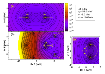
Figure 6: (Color online) The square of the denominator (panel (a)) and the numerator (panel (b)) of the S-matrix (Eq.(44)) for $d_{5/2}$ with $\langle\Delta\rangle=3.0$ MeV and $\lambda=-8.0$ MeV are shown on the complex quasiparticle energy plane. The yellow X-symbols show the position of zeros which represent the poles of the S-matrix. The yellow curves is the trajectories of zeros obtained by varying the pairing gap $\langle\Delta\rangle$ from 0.0 to 10.0 MeV. The arrows represent the direction of X.

The T-matrix for the neutron elastic scattering on open-shell nucleus can be derived as

$$T_{lj}(E)\equiv\frac{i}{2}\left(S_{lj}^{11}(E)-1\right)$$

$$=\frac{i}{2}\sum_{s=1,2}\left(\mathcal{J}_{lj}^{(+)}(E)\right)^{-1}_{1s}\left[\left(\mathcal{J}_{lj}^{(-)}(E)\right)_{s1}-\left(\mathcal{J}_{lj}^{(+)}(E)\right)_{s1}\right]$$

$$=\frac{2mk_{1}(E)}{\hbar^{2}}\int_{0}^{\infty}dr\chi_{l}^{(r1)\mathrm{T}}(r;E)\mathcal{U}_{lj}(r)\psi_{lj}^{(+)}(r;E).$$ (60)

Note that Eqs.(34) and (41) was used to derive Eq.(60).

When the S-matrix satisfies the Unitarity (Eq.(56), the T-matrix satisfies the optical theorem given by

$$-\mbox{ Im }T_{lj}(E)=|T_{lj}(E)|^{2},$$ (61)

where $E$ is supposed to be existing on the branch cut. The total cross section for nucleon scattering $\sigma_{lj}(\hbar\omega)$ is given by

$$\sigma(E_{i}) = \sum_{lj}\sigma_{lj}(E_{i}),$$ (62)

$$\sigma_{lj}(E_{i}) = \frac{\hbar^{2}}{2m}\frac{\pi}{E_{i}}\frac{2j+1}{2}|T_{lj}(E_{i}-\lambda)|^{2},$$ (63)

where $E_{i}$ is the incident nucleon energy defied by

$$E_{i}=E+\lambda.$$ (64)

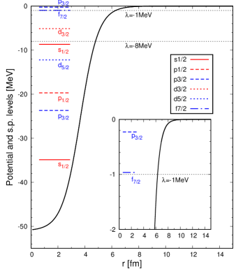
Figure 7: (Color online) The Woods-Saxon potential and the single-particle levels obtained in the no pairing limit. The lines of Fermi energy $\lambda=-1$ and $-8$ MeV are displayed together.

IV Numerical results

In this study, we adopt the Woods-Saxon potential which is given by

$$U_{lj}(r) = \left[V_{0}+V_{ls}\mbox{\boldmath$l$}\!\cdot\!\mbox{\boldmath$s$}\frac{r_{0}^{2}}{r}\frac{d}{dr}\right]f(r),$$ (65)

$$f(r) = \frac{1}{1+\exp\left(\frac{r-R}{a}\right)},$$ (66)

in the standard form for the Hartree-Fock mean field $U_{lj}(r)$ in Eq.(1) with use of the standard parameters given by hamamoto ; bohr . The mass number $A=24$ is used for the parameter given by $R=r_{0}A^{\frac{1}{3}}$.

The volume-type pairing field $\Delta(r)$ described by

$$\Delta(r)=V_{pair}f(r)$$ (67)

is adopted in the paper.

We define the average pairing gap $\langle\Delta\rangle$ by

$$\langle\Delta\rangle\equiv\frac{\int r^{2}dr\Delta(r)f(r)}{\int r^{2}drf(r)},$$ (68)

as introduced in hamamoto . We solve the integral equation Eq.(27) numerically, and obtain $\phi_{lj}^{(\pm s)}(r;E)(s=1,2)$ in order to calculate the Jost function with Eq.(35) in this study. It should be noted that we confirmed that the Jost function by Eqs.(34)-(36) give the same numerical results.

The square of the denominator (panel (a)) and the numerator (panel (b)) of the S-matrix (Eq.(44)) for $d_{5/2}$ with $\langle\Delta\rangle=3.0$ MeV and $\lambda=-8.0$ MeV are shown on the complex quasiparticle energy plane in Fig.6. The yellow colored X-symbols are zeros of the plotted function determined by the Nelder-Mead method nelder . The yellow curves are the trajectories of the S-matrix poles with varying $\langle\Delta\rangle$ from 0.0 to 10.0 MeV. The arrows represent the direction of motion of zeros indicated by X-symbols.

The same results are shown on the complex $k_{1}$-plane in Fig.8. Panels (a) and (b) in Fig.6 correspond to the (a)upper and (b)lower figures in Fig.8, respectively. The dashed curves seen in the upper-half and lower-half plane represent Re $E=0$ which pass through the points at $k_{1}=\pm ik_{F}$. $k_{F}$ is the Fermi momentum defined by $k_{F}\equiv\sqrt{\frac{2m|\lambda|}{\hbar^{2}}}$. The above/below regions on upper/lower panels is corresponding to the negative energy regions (left-half planes) of 1st/2nd Riemann sheets, respectively, as explained in Figs.1 and 2.

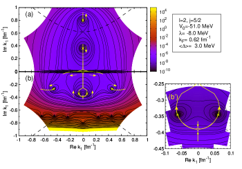
Figure 8: (Color online) The same figure with Fig.6 but on the complex $k_{1}$-momentum plane. The upper- and lower-half plane ((a) and (b)) correspond to the panels (a) and (b) in Fig.6, respectively. The dashed curves show curves where Re $E=0$ MeV.

The S-matrix poles on the 1st Riemann sheet are existing on the real axis, and have a tendency to go away from $E=0$ along the real axis. Corresponding poles on $k_{1}$-momentum plane are existing on the imaginary axis and go away from the Fermi momentum along the imaginary axis as the pairing gap is increased.

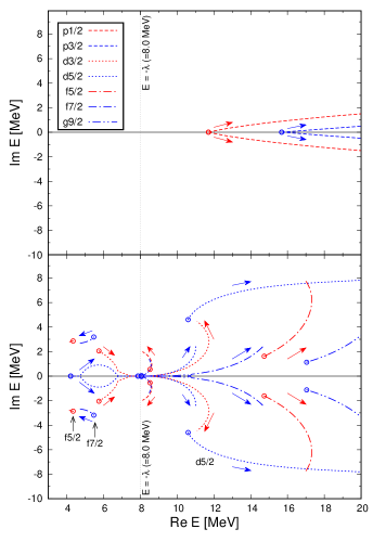
Figure 9: (Color online) Trajectories of the S-matrix poles on the 2nd Riemann sheet with varying the pairing gap $\langle\Delta\rangle$ from 0 to 10 MeV. o-symbols represent the position of poles at the no pairing limit ($\langle\Delta\rangle=0$ MeV). The hole-like and particle-like poles are classified in the upper and lower panels, respectively (see text).

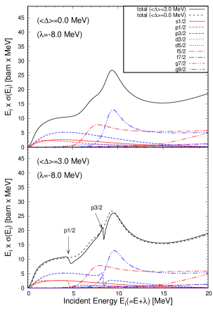
Figure 10: (Color online) The total cross section and the partial cross sections for the neutron elastic scattering with $\lambda=-8.0$ MeV.

The S-matrix poles existing on the real axis of the 2nd Riemann sheet move along the real axis by taking a circular trajectory as the pairing gap is increased. It seems to avoid a certain point existing around $E=-\frac{3}{4}\lambda=6$ MeV shown as (b’) in Fig.6. The certain point corresponds to $k_{1}=-ik_{F}/2$ on the complex $k_{1}$-momentum plane. The poles become resonances at $E>-\lambda$ with the large pairing gap limit. We need further investigation in order to clarify this point.

The resonances which are found at $E=10.60\pm 4.60\hskip 2.0pti$ MeV with $\Delta(r)=0$ move on the trajectories as shown in Fig.6 due to the pairing effect. The trajectory of resonances show that the pairing effect increases both resonance energy and width, since the imaginary value of the pole on the complex energy plane corresponds to the width of resonance.

In Fig.9, we show the trajectories of S-matrix all poles existing on the 2nd Riemann sheet below 20 MeV quasiparticle energy obtained by varying the pairing gap $\langle\Delta\rangle$ from 0 to 10 MeV. It seems to be possible to classify the trajectories from their behaviour into two types except the poles of $d_{5/2}$, $f_{5/2}$ and $f_{7/2}$ denoted by the text in Fig.9. The $p_{1/2}$ and $p_{3/2}$ poles shown in the upper panel become resonances by the configuration mixing between hole states existing below the Fermi energy as shown in Fig.7 and the continuum states due to the pairing effect. The resonance energy and the width are monotonically increased as the pairing gap is increased. This type of the resonances are called as “hole-like” quasiparticle resonance kobayashi .

The resonances above $E=-\lambda(=8$MeV) are called as the “particle-like” quasiparticle resonances in kobayashi . The resonances at the no pairing limit are formed by the centrifugal barrier and the spin-orbit potential. Such resonances are called as “the shape resonance”. The trajectories in the lower panel above $E=-\lambda(=8$MeV) show the pairing effect on the “shape resonance” except the $d_{5/2}$ resonance which is represented by text in the figure with large width.

The poles of $d_{5/2}$ and $d_{3/2}$ existing below $E=-\lambda(=8$MeV) are anti-bound quasiparticle states. These poles are moved to the positive direction of the real axis, and become the “particle-like” quasiparticle resonance above $E=-\lambda(=8$MeV) at the large pairing limit.

Table 1: S-matrix poles of hole-like quasiparticle resonances which give the clear contribution to the total cross section shown in Fig.10.

$\langle\Delta\rangle$	$p_{1/2}$	$p_{3/2}$
$0.0$	$11.71$	$15.68$
$3.0$	$12.65\pm i0.28$	$16.39\pm i0.08$

(For $\lambda=-8.0$ MeV, Unit:MeV)

The trajectory’s behaviour of the poles of $d_{5/2}$, $f_{5/2}$ and $f_{7/2}$ denoted by the text in Fig.9 is distinct from both “particle-like” and “hole-like” resonances. The $d_{5/2}$ resonance may contribute to the nucleon scattering cross section as a background because it has very wide width. These states may be categorized into “echo” state of the nucleon scattering as suggested by Sasakawa sasakawa . However, more detailed analysis of these poles would be necessary to determine the classification.

We show the total neutron elastic scattering cross section as a function of the incident energy of neutron defined by Eq.(64) in Fig.10. The partial cross sections for each angular momentum components are also shown in the same figure. We use the formulas given by Eqs.(62) and (63) to calculate the cross section. The incident energy $E_{i}$ is multiplied to the cross section in order to see the contribution of the partial cross section clearly. The cross sections with $\langle\Delta\rangle=0$ and $3.0$ MeV are shown in the upper and lower panels, respectively. In the lower panel, the total cross section with $\langle\Delta\rangle=0$ MeV is also plotted by the black dashed curve for comparison.

A peak found around $E_{i}\sim 9.5$MeV in the upper panel is a typical shape resonances formed by $g_{9/2}$ and $f_{5/2}$ resonances. It is very difficult to see the pairing effect on those resonances in comparison between the upper and lower panel because those resonances have wide width and the energy shift is also very small. On the other hand, we can find staggering shapes of cross section around $E_{i}\sim 4.5$ and $8$ MeV. Those staggering shapes of cross section are due to the asymmetric shapes of the partial cross section caused by the hole-like quasiparticle resonances of $p_{1/2}$ and $p_{3/2}$, respectively. The quasiparticle energies found on the 2nd Riemann sheet of the complex quasiparticle energy plane are listed in Table 1. The widths for each resonances, $p_{1/2}$ and $p_{3/2}$, are determined as $\Gamma=0.56,0.16$ MeV respectively, because Im $E=\frac{\Gamma}{2}$.

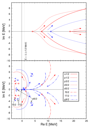
Figure 11: (Color online) The same figure with Fig.9 but with $\lambda=-1$ MeV.

Table 2: S-matrix poles of particle-like and hole-like quasiparticle resonances which give the clear contribution to the total cross section shown in Fig.12.

Particle-like
$\langle\Delta\rangle$	$p_{3/2}$	$f_{7/2}$
$0.0$	$0.89$	$0.91\pm i0.11$
$3.0$	$1.35\pm i0.17$	$2.46\pm i0.01$

Hole-like
$\langle\Delta\rangle$	$d_{3/2}$	$s_{1/2}$	$d_{5/2}$	$p_{1/2}$
$0.0$	$4.12$	$7.69$	$11.22$	$18.70$
$3.0$	$4.98\pm i0.26$	$8.30\pm i0.48$	$11.84\pm i0.33$	$19.29\pm i0.03$

(For $\lambda=-1.0$ MeV, Unit:MeV)

In Fig.11, we show the same plot for the case of $\lambda=-1.0$ MeV to see the trajectories of the S-matrix poles for the neutron-rich unstable nuclei. The number of the hole-like quasiparticle resonances shown in the upper panel are increased because of the shallow Fermi energy. The paring effect on the particle-like quasiparticle resonances ($p_{1/2}$, $p_{3/2}$, $f_{5/2}$ and $g_{9/2}$) are same qualitatively in shape or form of the trajectories, but more sensitive to the pairing gap than those shown in Fig.9. The $d_{5/2}$-resonance indicated by text in the Fig.11 is existing with the same width in the no pairing limit as the one shown in Fig.9. However, the sensitivity for the pairing is quite different. Almost no pairing effect can be seen in the behaviour of $d_{5/2}$-resonance trajectory even at the large pairing limit ($\langle\Delta\rangle=10.0$ MeV).

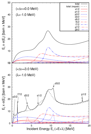
Figure 12: (Color online) The total cross section and the partial cross sections for the neutron elastic scattering with $\lambda=-1.0$ MeV.

The total cross section for the neutron elastic scattering is shown in Fig.12. The partial cross sections for each angular momentum are also shown together. In the lower panel, we can find 6 peaks of resonances which are caused by the pairing effect. The two peaks indicated as $p_{3/2}$ and $f_{7/2}$ are the particle-like quasiparticle resonances. The 4 peaks indicated by text as $s_{1/2}$, $p_{1/2}$, $d_{3/2}$ and $d_{5/2}$ in Fig.11 are the hole-like quasiparticle resonances corresponding the S-matrix poles represented in the upper panel of Fig.11. The corresponding quasiparticle energies on the complex quasiparticle energy plane are listed in Table 2. The widths for each resonances can be obtained by multiplying factor $2$ to the imaginary values of the complex quasiparticle energies.

V summary

We have extended the Jost function formalism based on the Hartree-Fock-Bogoliubov formalism in order to give the analytic expression of the S-matrix for the nucleon elastic scattering targeting on the open-shell nucleus. We showed that the S-matrix satisfies the unitarity on the branch-cut (continuum) in the positive quasiparticle energy region. Adopting the Woods-Saxon potential, we showed the S-matrix poles on the complex quasiparticle energy/momentum plane by using the analytic expression of the S-matrix represented by the Jost function. The trajectories of the S-matrix poles obtained by varying the pairing strength were also shown for two cases of the Fermi energies given by $\lambda=-8.0$ and $-1.0$ MeV. We pointed out that the trajectories of resonances can be categorized into two types, the hole-like and particle-like quasiparticle resonances aside from a couples of exceptions. We confirmed that such quasiparticle resonances can be observed as the staggering shape or sharp peaks of the total cross section of the neutron elastic scattering. We did not compare our results with the experimental data in this study. For the quantitative discussion, we need to adopt the proper optical potential in order to take account the proper absorption given by the imaginary part of the optical potential. One of the proper way is to adopt the microscopic optical potential based on the PVC method. However, it may be necessary to extend the existing the PVC method to the quasiparticle-vibration coupling method for the self-consistency of the method although it is a matter of concern that excessive calculation time is required. An alternative way is to adopt the GOP, however, readjustment of the parameters may be necessary because the current parameters have been adjusted without pairing correlation.

VI Acknowledgments

We thank Dr. Yoshihiko Kobayashi (Kyushu University) for useful discussions. This work is funded by Vietnam National Foundation for Science and Technology Development (NAFOSTED) under grant number “103.04-2018.303”. T. Dieu Thuy partially thanks the financial support of the Nuclear Physics Research Group (NP@HU) at Hue University through the Hue University Grant 43/HD-DHH.

References

- (1) R. Jost and A. Pais, Phys. Rev. 82, 840 (1951).
- (2) L. F. Canto, M. S. Hussein, Sacattering theory of Molecules, Atoms and Nuclei, (World Scientific, Singapore, 2013).
- (3) J. I. Roeder, Ann. Phys. 43, 382-409 (1967).
- (4) H. A. Weidenmuller, Ann. Phys. 28, 60-115 (1964).
- (5) B. A. Watson, P. P. Singh, and R. E. Segel, Phys. Rev. 182, 977 (1969).
- (6) F. D. Becchetti, Jr., and G. W. Greenlees, Phys. Rev. 182, 1190 (1969).
- (7) A. Nadasen, et al., Phys. Rev. C 23, 1023 (1981).
- (8) R. L. Varner, et al., Phys. Rep. 201, 57(1991).
- (9) S. Hama, et al., Phys. Rev. C 41, 2737 (1990).
- (10) E. D. Cooper, S. Hama, B. C. Clark, and R. L. Mercer, Phys. Rev. C 47, 297 (1993).
- (11) A. J. Koning, J. P. Delaroche, Nucl. Phys. A 713 (2003) 231-310.
- (12) S. Kunieda, et al., J. Nucl. Sci. Technol. 44, 838 (2007).
- (13) Y. Han, et al., Phys. Rev. C 81, 024616 (2010).
- (14) C. M. Perey and F. G. Perey, Phys. Rev. 132, 755 (1963).
- (15) W. W. Daehnick, J. D. Childs, and Z. Vrcelj, Phys. Rev. C 21, 2253 (1980).
- (16) J. Bojowald, et al., Phys. Rev. C 38, 1153 (1988).
- (17) H. An and C. Cai, Phys. Rev. C 73, 054605 (2006).
- (18) Y. Han, Y. Shi, and Q. Shen, Phys. Rev. C 74, 044615 (2006).
- (19) H. Feshbach, Ann. Phys. 5 357 (1958).
- (20) Kazuhito Mizuyama, Kazuyuki Ogata, Phys. Rev. C 86, 041603(R), 2012.
- (21) Kazuhito Mizuyama, Kazuyuki Ogata, Phys. Rev. C 89, 034620 (2014).
- (22) G. Blanchon, et al., Phys. Rev. C 91, 014612 (2015).
- (23) T. V. Nhan Hao, Bui Minh Loc, and Nguyen Hoang Phuc, Phys. Rev. C 92, 014605 (2015).
- (24) A.M.Lane and R.G.Thomas, Rev. Mod. Phys. 30 257 (1958).
- (25) K. Shibata, et al., J. Nucl. Sci. Tech-nol. 48, 1–30 (2011).
- (26) www.oecd-nea.org/dbforms/data/eva/evatapes/jeff31.
- (27) M.B. Chadwick, et al., Nuclear Data Sheets 112, 2887–2996 (2011).
- (28) J. P. Svenne et al., Phys. Rev C 95, 034305 (2017).
- (29) M.-H. Koh, et al., Phys. Rev. C 95, 014315 (2017).
- (30) N. Schunck, et al., Phys. Rev. C 81, 024316 (2010).
- (31) N. Pillet, P. Quentin, and J. Libert, Nucl. Phys. A 697, 141 (2002).
- (32) T. V. Nhan Hao, P. Quentin, and L. Bonneau, Phys. Rev. C 86, 064307 (2012).
- (33) J. Dobaczewski, et al., Phys. Rev.C 53, 2809 (1996).
- (34) S. Fracasso and G. Colo, Phys. Rev. C 72, 064310 (2005).
- (35) J. Terasaki and J. Engel, Phys. Rev. C 82, 034326 (2010).
- (36) M. Matsuo, K. Mizuyama, and Y. Serizawa, Phys. Rev. C 71, 064326 (2005).
- (37) J. A. Nelder, R. Mead. Computer Journal 7(1965): 308–313.
- (38) I. Hamamoto and B. R. Mottelson, Phys. Rev. C 68, 034312 (2003).
- (39) I. Hamamoto and B. R. Mottelson, Phys. Rev. C 69, 064302 (2004).
- (40) Y. Zhang, M. Matsuo, and J. Meng, Phys. Rev. C 83, 054301 (2011).
- (41) Y. Kobayashi, M. Matsuo, Prog. Theor. Exp. Phys. 013D01 (2016).
- (42) M. Grasso, et al., Phys. Rev. C 64, 064321 (2000).
- (43) S. A. Fayans, S. V. Tolokonnikov, and D. Zawischa, Phys. Lett. B 491, 245 (2000).
- (44) N. Michel, K. Matsuyanagi, and M. Stoitsov, Phys. Rev. C 78, 044319 (2008).
- (45) J. C. Pei, A. T. Kruppa, and W. Nazarewicz, Phys. Rev. C 84, 024311 (2011).
- (46) Y. Zhang, M. Matsuo, and J. Meng, Phys. Rev. C 86, 054318 (2012).
- (47) H. Oba and M. Matsuo, Phys. Rev. C 80, 024301 (2009).
- (48) Y. N. Zhang, J. C. Pei, and F. R. Xu, Phys. Rev. C 88, 054305 (2013).
- (49) N. Sandulescu, N. V. Giai, and R. J. Liotta, Phys. Rev. C 61, 061301(R) (2000).
- (50) R. Id Betan, N. Sandulescu, and T. Vertse, Nucl. Phys. A 771, 93 (2006).
- (51) N. Sandulescu, et al., Phys. Rev. C 68, 054323 (2003).
- (52) S. Orrigo and H. Lenske, Phys.Lett.B 677 (2009)
- (53) Masayuki Matsuo and Yasuyoshi Serizawa, Phys. Rev. C 82, 024318 (2010).
- (54) A. Bohr and B. R. Mottelson, Nuclear Structure (Benjamin, New York, 1975), Vol. 1.
- (55) M. Matsuo, Nucl. Phys. A 696, 371 (2001).
- (56) S. A. Fayans, et al., Nucl. Phys. A 676,49 (2000).
- (57) S. T. Belyaev, et al., Sov. J. Nucl. Phys. 45 783 (1987).
- (58) Gustafson, K., (1998). Contemporary Mathematics, 218, 432–437.
- (59) T. Sasakawa, H. Okuno, S. Ishikawa, and T. Sawada,Phys. Rev. C 26, 42 (1982);T. Sasakawa Phys. Rev. C 28, 439 (1983);T. Sasakawa, “Scattering theory” (Shokabo, Tokyo,1991), ISBN978-4-7853-2321-9.