DFuseNet: Deep Fusion of RGB and Sparse Depth Information for Image Guided Dense Depth Completion
Abstract
In this paper we propose a convolutional neural network that is designed to upsample a series of sparse range measurements based on the contextual cues gleaned from a high resolution intensity image. Our approach draws inspiration from related work on super-resolution and in-painting. We propose a novel architecture that seeks to pull contextual cues separately from the intensity image and the depth features and then fuse them later in the network. We argue that this approach effectively exploits the relationship between the two modalities and produces accurate results while respecting salient image structures. We present experimental results to demonstrate that our approach is comparable with state of the art methods and generalizes well across multiple datasets.
I INTRODUCTION
Dense depth estimation is a critical component in autonomous driving, robot navigation and augmented reality. Popular sensing schemes in these domains involve a high resolution camera and a low resolution depth sensor such as a LiDAR or Time-of-Flight sensor. The density of points returned from commonly available depth sensors is typically an order of magnitude lower than the resolution of the camera image. Additionally, higher resolution variants of these sensors are expensive, making them impractical for most applications. However, a number of applications such as planning and obstacle avoidance can benefit from higher resolution range data which motivates us to consider approaches that can up-sample the sparse available depth measurements to the resolution of the available imagery.
Traditionally, interpolation and diffusion based schemes have been used to up-sample sparse points into a smooth dense depth image, often using the corresponding color image as a guide [1]. Convolutional neural networks (CNN) have had tremendous success in depth estimation tasks using monocular image data [2, 3, 4, 5, 6, 7], stereo image data [8, 9, 10, 11] and sparse depth data on it’s own [12, 13, 14, 15].
One way to view both the monocular depth prediction problem and the depth completion problem is in terms of a posterior distribution which represents the probability of a given depth image, , given an input intensity image, . In both cases the approaches implicitly assume that the resulting posterior distribution is highly concentrated along a low dimensional manifold which makes it possible to infer the complete depth map from relatively few depth samples
We wish to design a CNN architecture that can learn sufficient global and contextual information from the color images and use this information along with sparse depth input to accurately predict depth estimates for the entire image, while enforcing edge preservation and smoothness constraints. Once designed, such a network could be used to upsample information from a variety of depth sensors including LiDAR systems, stereo algorithms or structure from motion algorithms. To summarize, we propose the following contributions:
-
1.
A CNN architecture that uses a dual branch architecture, spatial pyramid pooling layers and a sequence of multi-scale deconvolutions to effectively exploit contextual cues from the input color image and the available depth measurements.
-
2.
A training regime that can make of use different sources of information, such as stereo imagery, to learn how to extrapolate depth effectively in regions where no depth measurements are available.
-
3.
An evaluation of our methods on the KITTI Depth Completion Benchmark111http://www.cvlibs.net/datasets/kitti/eval_depth.php, virtual KITTI, NYUDepth, and our own mini-dataset. We show that our method is able to generalize well across these four different datasets.
-
4.
We also make our mini-dataset publicly available as it may serve as an additional source of validation data to the community. Details can be found in: https://github.com/ShreyasSkandanS/DFuseNet.
II RELATED WORK
Depth Estimation: Monocular depth estimation is an active research field where CNN based methods are currently the state of the art. Different methods have been proposed that use supervised [16, 17, 18, 19, 4, 3], unsupervised [2] and self-supervised [6] depth estimation strategies. At time of writing, the best performing monocular depth estimation algorithm is from Fu et al. , achieving an inverse RMSE score of 12.98 on the KITTI depth prediction dataset [7].
CNNs have been successfully used in dense stereo depth estimation tasks. Zbontar et al. proposed a siamese network architecture to learn a similarity measure between two input patches. This similarity measure is then used as a matching cost input for a traditional stereo pipeline [10]. Recently, many end-to-end methods have been proposed that are able to generate accurate disparity images while preserving edges [11, 8, 20, 21]. The work of Chang et al. is similar to the network we propose, where the authors propose an end-to-end approach using pyramid pooling to better learn global image dependent features [9].
Incomplete Input Data: Learning dense representations from sparse input is similar to the domain of super resolution and in-painting. Super resolution assumes that the input is a uniformly sub-sampled representation of the desired high resolution output, and the learning problem can be posed as an edge preserving interpolation strategy. A comprehensive review of these methods is presented by Yang et al. [22]. We note that multi-scale architectures with multiple skip connections have been successfully used for image and depth upsampling tasks [23, 24]. Content-aware completion is motivated by a similar problem of learning complete representations from incomplete input data. Image in-painting requires semantically aware completion of missing input regions. Generative networks have been used successfully for context aware image completion tasks [25, 26] but are outside the scope of this paper.
Depth Completion: A particular sub-problem of depth estimation with incomplete input data is depth completion. Following the release of the KITTI depth completion benchmark, novel approaches to solve the problem have been proposed. Uhrig et al. [12], the authors of the benchmark, propose a sparsity invariant CNN architecture, using partial normalized convolutions on the input sparse depth image. They propose multiple architectures that accommodate RGB information and sparse depth input only. Huang et al. propose HMSNet, which uses masked operations on the partial convolutions such as partial summation, up-sampling and concatenation [27].
Ku et al. propose a non-learning based approach to this problem to highlight the effectiveness of well crafted classical methods, using only commonly available morphological operations to produce dense depth information [14]. Their proposed method currently out-performs multiple deep learning based methods on the KITTI depth completion benchmark. Dimitrievski et al. propose a CNN architecture which uses the work of Ku et al. as a pre-processing step on the sparse depth input [28]. We followed a similar strategy and chose to fill in our sparse input depth image instead of using sparse convolutions. Their network is designed to use traditional morphological operators as well as subsequently learned morphological filters using a U-Net style architecture [29]. They are able to achieve better quantitative results but their model fails to preserve semantic and depth discontinuities as it relies heavily on the filled depth image for their final output. Eldesokey et al. propose a method that also uses normalized masked convolutions, but generates confidence values for each predicted depth by using a continuous confidence mask instead of a binary mask [15]. A similar confidence mask based approach is proposed by Gansbeke et al. [30]. Cheng et al. propose a depth propagation network to explicitly learn an affinity function and apply it to the depth completion problem [31].
Wang et al. propose a multi-scale feature fusion method for depth completion [32] using sparse LIDAR data. Ma et al. propose two methods, a supervised method for depth completion using a ResNet based architecture [13] and a self-supervised method [33] which uses the sparse LiDAR input along with pose estimates to add additional training information based on depth and photometric losses.
III Approach
III-A Design Overview
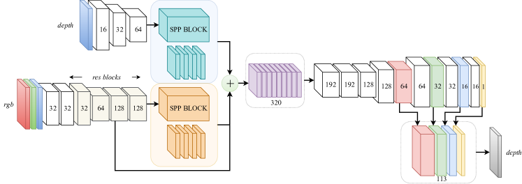
We propose the CNN architecture depicted in Figure 1. It has been structured to learn local to global context information from both the color image and the sparse depth data as well as to fuse them together to produce accurate and consistent dense depth maps. We propose a dual branch encoder design in a similar fashion to previous image comparison networks [10]. Given the differences in input modality provided to the two branches, we choose to not use Siamese networks with coupled weights [34], and instead use independent branches with different design decisions made for each branch. In our encoder, we use spatial pyramid pooling (SPP) blocks to learn a coarse-to-fine representation of features. Spatial pyramid pooling blocks have been effective in learning local to global context information and have been successfully used in depth perception tasks [9]. We concatenate features learned from individual branches and propagate these features through our de-convolution layers. The final layer performs a convolution operation on features combined from different de-convolution layers, up-sampled to the final output resolution, to utilize information from different scales and context to generate the final depth image.
III-B Feature Extraction
Our color and depth branches begin with an initial depth filling step, similar to the approach of Ku et al. [14]. We use a simple sequence of morphological operations and Gaussian blurring operations to fill the holes in the sparse depth image with depth values from nearby valid points such that no holes remain. This is then passed to the feature extraction branch. The filled depth image is then normalized by the maximum depth value in the dataset, resulting in depth values between 0 and 1. For the depth image, we choose to use larger kernel sizes and fewer convolution operations, resulting in fewer layers. For the color image, we use smaller kernel sizes and make use of four residual blocks [35], in addition to two initial convolution layers. The output of these initial feature extraction layers is then passed to spatial pyramid pooling (SPP) blocks. We use a similar structure to that proposed by Chang et al. [9], but use max pooling for our depth branch and average pooling for our color branch. Our pooling windows are consistent between the two branches and are 64, 32, 16 and 8 for each scale respectively. The output of this layer is an up-sampled stack of feature layers carrying information from different scales.


III-C Combining Modalities
The features from the previous extraction modules are then concatenated into one volume. The first layer is an intermediate output of the residual blocks from the color branch, which we hypothesize can carry over high level features learned from the color image. The subsequent layers are color and depth features extracted from the SPP blocks of the two branches. We believe that these layers can help learn a joint feature representation between the two input modalities in the following layers. We perform three sequential convolution operations on this volume, reducing the number of channels and increasing the spatial resolution by twice the size of the volume. By forcing a reduction in channels we attempt to force the network to learn a lower dimensional representation of the joint feature space, combining important information from both depth and color branches.
III-D Depth Prediction
The following layers perform a sequence of convolutions with batch normalization, and incremental de-convolutions to restore the original image resolution. The final step involves concatenating different layer outputs from the de-convolution pipeline, up-sampling by interpolation to achieve the original input resolution and then performing a final convolution on the multi-scale stack to produce a single channel output. This output is then passed to a sigmoid activation function and re-scaled to the original range of depth values. Odena et al. advise caution in the use of transposed convolutions for spatial upsampling [36], hence we limit the use of transposed convolutions and our final output is a result of a 1x1 convolution on a feature volume, which mainly consists of interpolated low resolution features, and hence minimizes the checkerboard effect in the final depth image.
III-E Training
Our training signal is a weighted average of multiple loss terms, some calculated over the entire image resolution and some calculated only at points where accurate ground truth depth exists. The weights , and are chosen based on a confidence associated with each signal and are varied at different points in time in the training regime.
| (1) |
III-E1 Primary Loss
We experimented with both L1 and L2 norms as primary loss functions . For this term, we calculate the loss only at pixels where ground truth depth exists and average over the total number of ground truth points. For better RMSE values on evaluation benchmarks we found L2 to be the better choice as a primary loss term.


III-E2 Optional Stereo Supervision
Since Uhrig et al. provide a large dataset with data from multiple cameras, we propose a means of making better use of this data during training. The KITTI depth completion dataset provides roughly 42k stereo image pairs, and we use these images to provide depth information at points where ground truth LiDAR data is missing. We propose an auxiliary loss term that uses the stereo input image pair to generate a dense depth estimate that can guide the learning process in regions where no ground truth LiDAR measurements exist. We compute this loss term in a self-supervised manner since stereo intrinsics and extrinsics are known. We use Semi Global Matching to generate this dense depth estimate [37]. This loss term is an L2 norm of the difference between the predicted depth and the stereo estimated depth. This term can be computed at almost every pixel in the input image. Some pixels lack depth estimates since we use left-right consistency checks to discard noisy and partially occluded depth estimates.


III-E3 Smoothness
IV EXPERIMENTS
Implementation Details: All our networks were implemented in PyTorch222http://pytorch.org and we train them from scratch, not using pre-trained weights for any layers. Our models are trained using the ADAM optimizer, and we typically use batch sizes of 20-25 for our experiments and train for roughly 40 epochs for all experiments. We use an initial learning rate of , and drop our learning rate by a factor of 10% after every 5 epochs. We use a weight decay term of . The weight terms from Eq 1 are: is usually set to 1, is 0.01 and is 0.001.
IV-A KITTI Depth Completion
The ground truth depth provided in the KITTI Depth Completion dataset is created by merging 11 LiDAR scans from frames before and after a given frame using pose estimates provided in the dataset [12]. These projected 3D points are refined using stereo depth estimation algorithms to discard outliers. During evaluation, the final scores are based only on these refined ground truth LiDAR points.
While this corpus provides a large amount of training data the available range measurements are typically clustered towards the bottom of the available imagery and are often missing at critical contextual regions such as object boundaries. A consequence is that models trained on this data often produce blurry edges since the available measurements and evaluation tools do not contraindicate such solutions.
Additionally the data set does not provide information in distant regions like the sky and many previous approaches involve cropping out regions where no LiDAR data is available. In contrast we seek to preserve as much contextual information as possible and make depth predictions across as much of the image as possible using all available data.
IV-A1 Quantitative Comparison
Our method achieves a mean RMSE score of and the current published state of the art is [30]. We are quantitatively out performed by Sparse-to-Dense [33], NConv-CNN [15], HMS-Net [27], CSPN [31] and MorphNet [28], but we believe that our model is able to better incorporate RGB image information to generate edge preserving and semantically smooth depth images at the cost of a small loss in metric accuracy. We highlight this in Figure 4, where it is clear that our method is able to use contextual information to preserve semantic boundaries as well as or better than methods that outperform us on the benchmark.
IV-A2 Learning to extrapolate with limited ground truth data
We validate the effectiveness of our stereo based loss term by comparing our model with and without this term. Quantitatively the improvements are minimal, i.e the model trains faster and results in slightly improved accuracy, qualitatively we noticed that our network can now extrapolate depth values at regions where no input LiDAR scan or ground truth exist. This is specially useful in datasets such as KITTI where the ground truth information is semi-dense with significant regions of the image missing ground truth LiDAR points. In Figure 3 we show a qualitative comparison of our network demonstrating its ability to extrapolate beyond the range of the LIDAR scans.
IV-B Virtual KITTI
We evaluate our network on the Virtual KITTI dataset [40]. This dataset contains roughly 21k image and depth frames generated in virtual worlds with simulated lighting and weather conditions, in a driving dataset similar to KITTI . The maximum depth range for this dataset is (sky), but for simplicity and similarity to our previous dataset, we set our perception limit to and train our model accordingly. We use 60% of this data as our training set and evaluate our model on the remaining images. To generate sparse depth input, we randomly sample 10% of the ground truth depth data uniformly. We apply the same input filling step as in the previous dataset, using the same parameters and morphological window sizes. We then pass this filled depth image along with the RGB image to our network and evaluate our accuracy in the - range.


While the virtual KITTI dataset is not an accurate representation of real life data, we show that our method is able to learn to accurately generate depth dense images, while preserving edges and contextual information. Figure 5 shows the our results on this dataset. We achieve an RMSE of and MAE of on our validation set.
IV-C NYU Depth V2
In our evaluation on the NYUDepthV2 dataset [41], we use the 1449 densely labelled pairs of aligned RGB and depth images, and split our dataset into 70% training and 30% validation. All our errors are reported on the 30% validation set and we compare our errors against the errors reported by other authors in their respective papers [31, 13, 42]. We use the full resolution 640480 images as our input and use the same method of subsampling as above to generate sparse input depth measurements from the ground truth. We use this dataset to verify that our model is able learn in different environments using different sources of input data, since here a Kinect RGBD sensor is used to collect data in various common environments such as offices and homes.
Table I shows the performance of our model at multiple levels of sparsity compared to the work of Ma et al. and Liao et al. at 200 samples [13, 42]. Our approach performs comparably to the the approach of Ma et al. and better than that of Liao et al. . We use the same morphological window size and operations as in the Virtual KITTI and KITTI datasets and our method is able to generate accurate results even with noisy input filling. Again the filling process helps us by removing all zeros in the depth image and providing a reasonable initialization but the final depth prediction is based on the combined features from the RGB and depth branches of the network. It must be noted here that the results reported here were computed using a different randomly chosen set of samples and a direct comparison would be unfair.
| Method - No. of samples | RMSE | REL | |||
|---|---|---|---|---|---|
| DFuseNet (ours) - 200 | 0.2966 | 0.0609 | 0.9588 | 0.9927 | 0.9982 |
| DFuseNet - 500 | 0.2195 | 0.0441 | 98.04 | 99.70 | 99.93 |
| DFuseNet - 1k | 0.1759 | 0.0371 | 98.78 | 99.82 | 99.96 |
| Cheng et.al (rgbd) [31] - 500 | 0.117 | 0.016 | 99.2 | 99.9 | 100.0 |
| Ma et al. (rgbd) [13] - 200 | 0.230 | 0.044 | 97.1 | 99.4 | 99.8 |
| Liao et al. (rgbd) [42] - 225 | 0.442 | 0.104 | 87.8 | 96.4 | 98.9 |
IV-D Number of depth samples
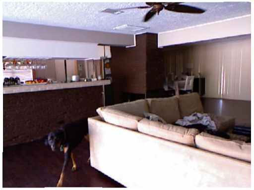
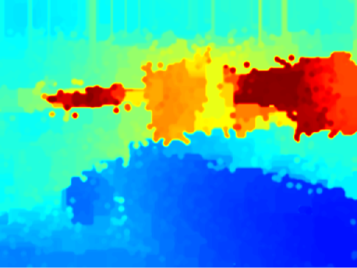
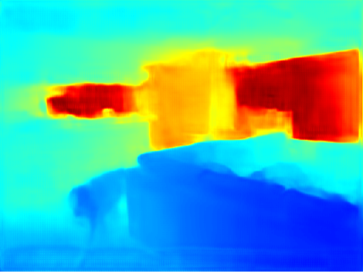
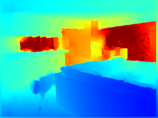
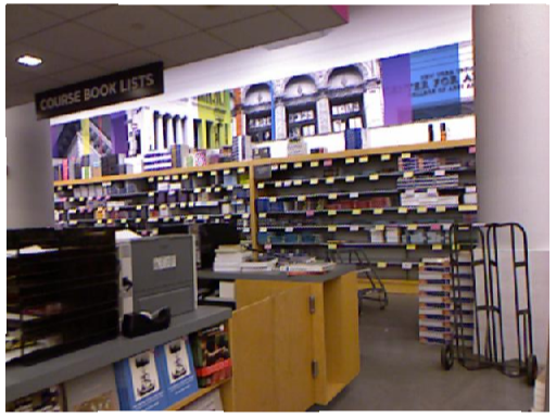
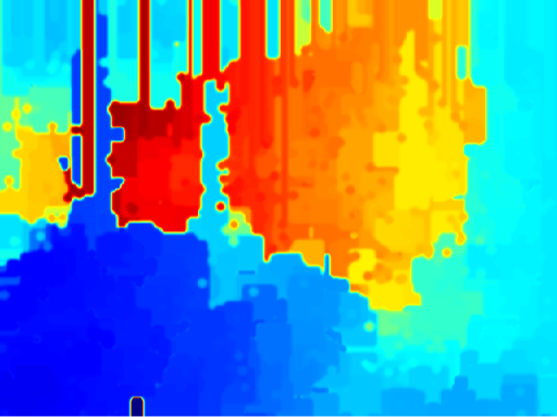
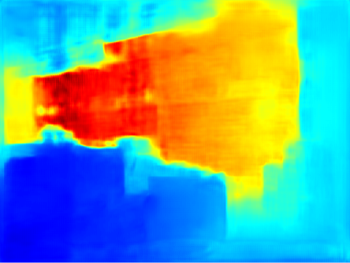
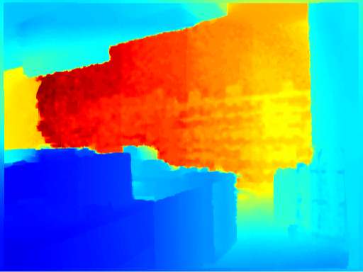
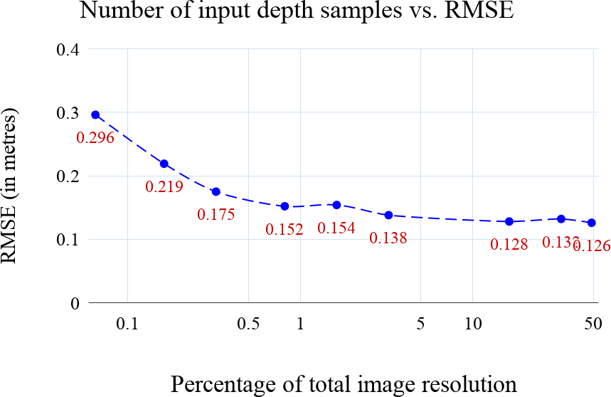
For this experiment, we use the NYUDepthV2 dataset as we are provided with dense ground truth information resulting in more consistent accuracy results. We train a different model for every sample size, limiting the training time to a fixed number of epochs each. We initialize our model with weights learned from our KITTI Depth Completion dataset to reduce our training time. We evaluate RMSE values on our validation set and a plot of this can be seen in Figure 7. As observed by Ma et al. in their network, the performance gained by adding more sparse input samples tends to saturate. We notice a saturation at around 5000 depth samples, roughly 1.7% of the image resolution. Qualitatively we can see in Figure 6 that even with an extremely sparse input sample set, the RGB branch of our network is able to guide the depth prediction using mostly image based contextual cues.
IV-E Penn Driving LiDAR RGB Dataset
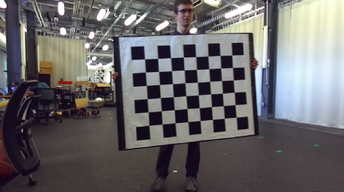
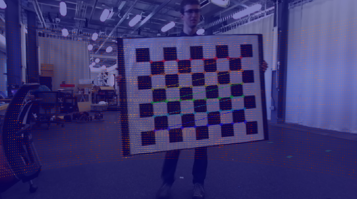

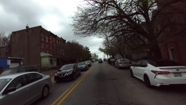
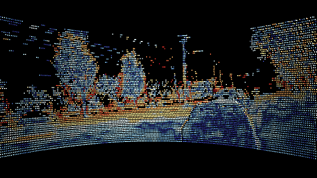
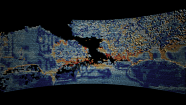
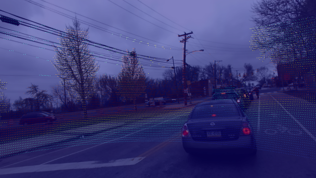
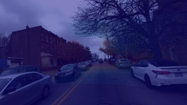
We additionally test this model on our own well-calibrated LiDAR and RGB dataset. We use an Ouster OS-1333http://www.ouster.io 64 beam LiDAR along with a StereoLabs Zed Mini444https://www.stereolabs.com/zed-mini/ camera. In order to calibrate the extrinsics between the LiDAR and camera, we utilize the intensity image from the Ouster. We detect checkerboard corners in the intensity image, and then project them into the point cloud to find their locations in 3 dimensional space. These points can then be projected back onto a virtual image plane located in front of the LiDAR and standard stereo calibration tools can be used to calibrate the virtual LiDAR camera to the RGB camera. We finally project the LiDAR point cloud onto the RGB image in order to verify the calibration, as shown in Figure 8
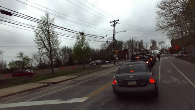
Following calibration, we mounted the camera and LiDAR assembly to a car and collected 15 minutes of driving in downtown Philadelphia. We artificially remove points from the point cloud to simulate a lower resolution sensor and run our pre-trained model. This translates to 5000 randomly sampled points from roughly 40,000 LiDAR points. The withheld points are then used for evaluating inference accuracy.
V Discussion and Conclusion
In this section we discuss our observations and the motivation behind our design decisions in the context of datasets such as KITTI and NYU Depth.
V-A Architecture
Jaritz et al. talk briefly about the benefits of a late fusion architecture over an early fusion one [43]. We agree with their statement and reaffirm the belief that given the different representations of RGB and depth modalities, the correct way to jointly combine this information is by learning to first transform it into a common feature space. While previous work has proposed single path architectures, where RGB and the sparse depth channels are concatenated into a single 4D input and passed to a network [13], we propose the use of a number of individual and independent convolution and pyramid pooling operators on the individual modalities in a dual branch manner. We experimented with implementations where both modalities were fused prior to the SPP blocks and noticed a drop in performance, hinting that the additional independent information learned was useful to the final fusion and prediction. Figure 2 shows the information gained from having two branches in our network.
In terms of input sparsity, we experimented with replacing all our convolutions in the depth branch with sparse convolutions [12] but noticed a significant drop in performance. Huang et al. propose the use of additional sparse operations such as sparsity invariant upsampling, addition and concatenation in addition to convolution and were able to achieve much better results [27]. However, we are more inclined to believe that desirable performance can be achieved with the use of regular convolutions and operations for multi-modal input with simple pre-processing hole filling operations such as morphological filters, fill maps and nearest neighbor interpolation [28, 14, 44]. This is simple and effective in providing the network with a good initialization.
We did notice however that with hole filling pre-processing steps, care must be taken in the use of residual connections from the depth channels to the penultimate layers. We found that using a residual connection from the second and third layers of our depth channel to the penultimate layer of our deconvolution layers led to similar accuracy as IPBasic [14] but the network failed to learn to use information from the RGB branch. Perhaps such a network must be more carefully trained with carefully selected hyperparameters. However, in a single channel or early fusion network, adding residual connections from the depth input to the final layers has been shown to be highly effective [33, 31].
V-B Generalization
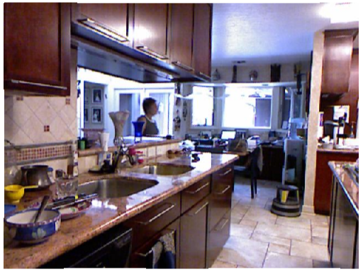
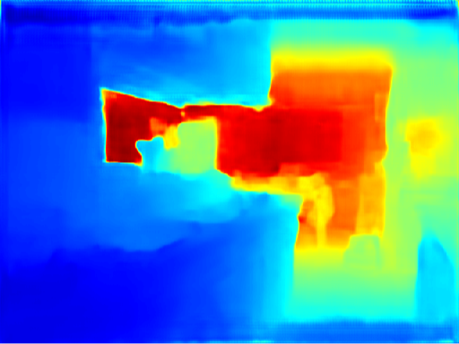
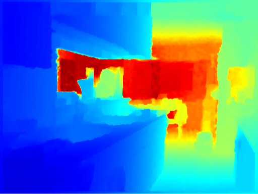
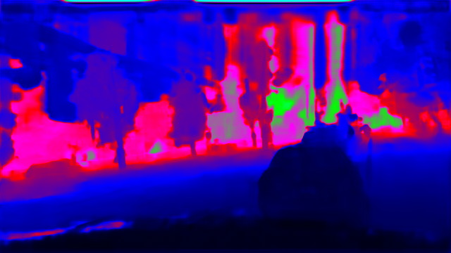
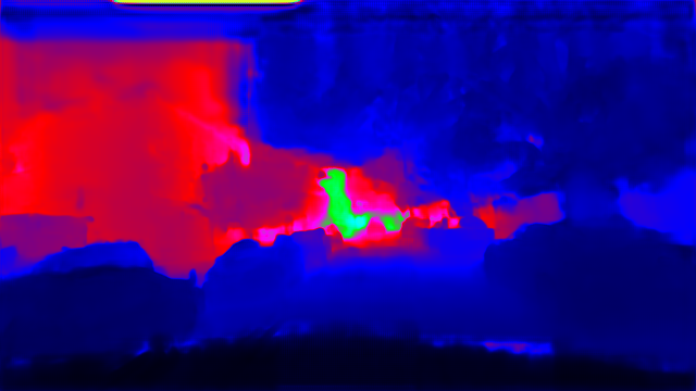
We also test the model we trained for the KITTI Depth Completion benchmark on Virtual KITTI, our Penn Driving dataset and NYUDepthV2. Figure 9 shows a few examples of predictions made using our KITTI Depth Completion model on Virtual Kitti and NYUDepthV2. Qualitatively, we noticed that the network is able to use sufficient RGB cues to generate semantically valid depth predictions but quantitatively we noticed errors in predicted depth values. This is due to the difference in depth scale across the three datasets (KITTI maximum depth is , virtual kitti is and NYUDepth is roughly ) and is quickly corrected after minimal training using the KITTI model as an initialization. We believe that the separate RGB image branch and the density of features learned independently in this branch to be a large contributor to the generalization of this network. Our model trained on KITTI is able to achieve an RMSE value of and MAE of on our NYUDepthV2 test set using 10% of ground truth as input depth samples. On the Penn driving dataset, we achieved an RMSE of and MAE of . The higher error is mainly in regions far away as shown in the error images in Figure 10.



V-C Conclusion
We have proposed a CNN architecture that can be used to upsample sparse range data using the available high resolution intensity imagery. Our architecture is designed to extract contextual cues from the image to guide the upsampling process which leads to a network with separate branches for the image and depth data. We have demonstrated its performance on relevant datasets and shown that the approach appears to capture salient cues from the image data and produce upsampled depth results that respect relevant image boundaries and correlate well with the available ground truth. We also propose our own dataset for additional validation.
References
- [1] D. Ferstl, C. Reinbacher, R. Ranftl, M. Rüther, and H. Bischof, “Image guided depth upsampling using anisotropic total generalized variation,” in 2013 IEEE International Conference on Computer Vision. IEEE, 2013, pp. 993–1000.
- [2] C. Godard, O. Mac Aodha, and G. J. Brostow, “Unsupervised monocular depth estimation with left-right consistency,” in CVPR, vol. 2, no. 6, 2017, p. 7.
- [3] Z. Zhang, C. Xu, J. Yang, Y. Tai, and L. Chen, “Deep hierarchical guidance and regularization learning for end-to-end depth estimation,” Pattern Recognition, vol. 83, pp. 430–442, 2018.
- [4] B. Li, Y. Dai, and M. He, “Monocular depth estimation with hierarchical fusion of dilated cnns and soft-weighted-sum inference,” Pattern Recognition, 2018.
- [5] R. Li, K. Xian, C. Shen, Z. Cao, H. Lu, and L. Hang, “Deep attention-based classification network for robust depth prediction,” arXiv preprint arXiv:1807.03959, 2018.
- [6] Z. Li and N. Snavely, “Megadepth: Learning single-view depth prediction from internet photos,” in Computer Vision and Pattern Recognition (CVPR), 2018.
- [7] H. Fu, M. Gong, C. Wang, K. Batmanghelich, and D. Tao, “Deep ordinal regression network for monocular depth estimation,” in IEEE Conference on Computer Vision and Pattern Recognition (CVPR), 2018.
- [8] X. Song, X. Zhao, H. Hu, and L. Fang, “Edgestereo: A context integrated residual pyramid network for stereo matching,” arXiv preprint arXiv:1803.05196, 2018.
- [9] J.-R. Chang and Y.-S. Chen, “Pyramid stereo matching network,” in IEEE Conference on Computer Vision and Pattern Recognition, 2018.
- [10] J. Zbontar and Y. LeCun, “Stereo matching by training a convolutional neural network to compare image patches,” Journal of Machine Learning Research, vol. 17, no. 1-32, p. 2, 2016.
- [11] A. Kendall, H. Martirosyan, S. Dasgupta, and P. Henry, “End-to-end learning of geometry and context for deep stereo regression,” in Computer Vision (ICCV), 2017 IEEE International Conference on. IEEE, 2017, pp. 66–75.
- [12] J. Uhrig, N. Schneider, L. Schneider, U. Franke, T. Brox, and A. Geiger, “Sparsity invariant cnns,” in 2017 International Conference on 3D Vision (3DV). IEEE, 2017, pp. 11–20.
- [13] F. Ma and S. Karaman, “Sparse-to-dense: Depth prediction from sparse depth samples and a single image,” in 2018 IEEE International Conference on Robotics and Automation (ICRA). IEEE, 2018, pp. 1–8.
- [14] J. Ku, A. Harakeh, and S. L. Waslander, “In defense of classical image processing: Fast depth completion on the cpu,” arXiv preprint arXiv:1802.00036, 2018.
- [15] A. Eldesokey, M. Felsberg, and F. S. Khan, “Propagating confidences through cnns for sparse data regression,” arXiv preprint arXiv:1805.11913, 2018.
- [16] D. Eigen, C. Puhrsch, and R. Fergus, “Depth map prediction from a single image using a multi-scale deep network,” in Advances in neural information processing systems, 2014, pp. 2366–2374.
- [17] F. Liu, C. Shen, G. Lin, and I. D. Reid, “Learning depth from single monocular images using deep convolutional neural fields.” IEEE Trans. Pattern Anal. Mach. Intell., vol. 38, no. 10, pp. 2024–2039, 2016.
- [18] W. Chen, Z. Fu, D. Yang, and J. Deng, “Single-image depth perception in the wild,” in Advances in Neural Information Processing Systems, 2016, pp. 730–738.
- [19] S. Kong and C. Fowlkes, “Pixel-wise attentional gating for parsimonious pixel labeling,” arXiv preprint arXiv:1805.01556, 2018.
- [20] G. Yang, H. Zhao, J. Shi, Z. Deng, and J. Jia, “Segstereo: Exploiting semantic information for disparity estimation,” in European Conference on Computer Vision. Springer, 2018, pp. 660–676.
- [21] S. Khamis, S. Fanello, C. Rhemann, A. Kowdle, J. Valentin, and S. Izadi, “Stereonet: Guided hierarchical refinement for real-time edge-aware depth prediction,” in European Conference on Computer Vision. Springer, 2018, pp. 596–613.
- [22] C.-Y. Yang, C. Ma, and M.-H. Yang, “Single-image super-resolution: A benchmark,” in European Conference on Computer Vision. Springer, 2014, pp. 372–386.
- [23] J. Yamanaka, S. Kuwashima, and T. Kurita, “Fast and accurate image super resolution by deep cnn with skip connection and network in network,” in Neural Information Processing. Springer, 2017, pp. 217–225.
- [24] T.-W. Hui, C. C. Loy, and X. Tang, “Depth map super-resolution by deep multi-scale guidance,” in European Conference on Computer Vision. Springer, 2016, pp. 353–369.
- [25] R. A. Yeh, C. Chen, T.-Y. Lim, A. G. Schwing, M. Hasegawa-Johnson, and M. N. Do, “Semantic image inpainting with deep generative models.” in CVPR, vol. 2, no. 3, 2017, p. 4.
- [26] J. Yu, Z. Lin, J. Yang, X. Shen, X. Lu, and T. S. Huang, “Generative image inpainting with contextual attention,” arXiv preprint, 2018.
- [27] Z. Huang, J. Fan, S. Yi, X. Wang, and H. Li, “Hms-net: Hierarchical multi-scale sparsity-invariant network for sparse depth completion,” arXiv preprint arXiv:1808.08685, 2018.
- [28] M. Dimitrievski, P. Veelaert, and W. Philips, “Learning morphological operators for depth completion,” in International Conference on Advanced Concepts for Intelligent Vision Systems. Springer, 2018, pp. 450–461.
- [29] O. Ronneberger, P. Fischer, and T. Brox, “U-net: Convolutional networks for biomedical image segmentation,” in International Conference on Medical image computing and computer-assisted intervention. Springer, 2015, pp. 234–241.
- [30] W. Van Gansbeke, D. Neven, B. De Brabandere, and L. Van Gool, “Sparse and noisy lidar completion with rgb guidance and uncertainty,” arXiv preprint arXiv:1902.05356, 2019.
- [31] X. Cheng, P. Wang, and R. Yang, “Depth estimation via affinity learned with convolutional spatial propagation network,” in European Conference on Computer Vision. Springer, 2018, pp. 108–125.
- [32] B. Wang, Y. Feng, and H. Liu, “Multi-scale features fusion from sparse lidar data and single image for depth completion,” Electronics Letters, 2018.
- [33] F. Ma, G. V. Cavalheiro, and S. Karaman, “Self-supervised sparse-to-dense: Self-supervised depth completion from lidar and monocular camera,” arXiv preprint arXiv:1807.00275, 2018.
- [34] J. Bromley, I. Guyon, Y. LeCun, E. Säckinger, and R. Shah, “Signature verification using a” siamese” time delay neural network,” in Advances in neural information processing systems, 1994, pp. 737–744.
- [35] K. He, X. Zhang, S. Ren, and J. Sun, “Deep residual learning for image recognition,” in Proceedings of the IEEE conference on computer vision and pattern recognition, 2016, pp. 770–778.
- [36] A. Odena, V. Dumoulin, and C. Olah, “Deconvolution and checkerboard artifacts,” Distill, 2016. [Online]. Available: http://distill.pub/2016/deconv-checkerboard
- [37] H. Hirschmuller, “Accurate and efficient stereo processing by semi-global matching and mutual information,” in Computer Vision and Pattern Recognition, 2005. CVPR 2005. IEEE Computer Society Conference on, vol. 2. IEEE, 2005, pp. 807–814.
- [38] T. Zhou, M. Brown, N. Snavely, and D. G. Lowe, “Unsupervised learning of depth and ego-motion from video,” in CVPR, vol. 2, no. 6, 2017, p. 7.
- [39] S. Vijayanarasimhan, S. Ricco, C. Schmid, R. Sukthankar, and K. Fragkiadaki, “Sfm-net: Learning of structure and motion from video,” arXiv preprint arXiv:1704.07804, 2017.
- [40] A. Gaidon, Q. Wang, Y. Cabon, and E. Vig, “Virtual worlds as proxy for multi-object tracking analysis,” in Proceedings of the IEEE conference on computer vision and pattern recognition, 2016, pp. 4340–4349.
- [41] N. Silberman, D. Hoiem, P. Kohli, and R. Fergus, “Indoor segmentation and support inference from rgbd images,” in European Conference on Computer Vision. Springer, 2012, pp. 746–760.
- [42] Y. Liao, L. Huang, Y. Wang, S. Kodagoda, Y. Yu, and Y. Liu, “Parse geometry from a line: Monocular depth estimation with partial laser observation,” in Robotics and Automation (ICRA), 2017 IEEE International Conference on. IEEE, 2017, pp. 5059–5066.
- [43] M. Jaritz, R. De Charette, E. Wirbel, X. Perrotton, and F. Nashashibi, “Sparse and dense data with cnns: Depth completion and semantic segmentation,” in 2018 International Conference on 3D Vision (3DV). IEEE, 2018, pp. 52–60.
- [44] Z. Chen, V. Badrinarayanan, G. Drozdov, and A. Rabinovich, “Estimating depth from rgb and sparse sensing,” arXiv preprint arXiv:1804.02771, 2018.