Asymmetric Valleys: Beyond Sharp and Flat Local Minima

Haowei He    Gao Huang    Yang Yuan
Abstract

Despite the non-convex nature of their loss functions, deep neural networks are known to generalize well when optimized with stochastic gradient descent (SGD). Recent work conjectures that SGD with proper configuration is able to find wide and flat local minima, which have been proposed to be associated with good generalization performance. In this paper, we observe that local minima of modern deep networks are more than being flat or sharp. Specifically, at a local minimum there exist many asymmetric directions such that the loss increases abruptly along one side, and slowly along the opposite side – we formally define such minima as asymmetric valleys. Under mild assumptions, we prove that for asymmetric valleys, a solution biased towards the flat side generalizes better than the exact minimizer. Further, we show that simply averaging the weights along the SGD trajectory gives rise to such biased solutions implicitly. This provides a theoretical explanation for the intriguing phenomenon observed by Izmailov et al. (2018). In addition, we empirically find that batch normalization (BN) appears to be a major cause for asymmetric valleys.

SGD, Landscape, Non-convex optimization

1 Introduction

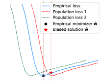
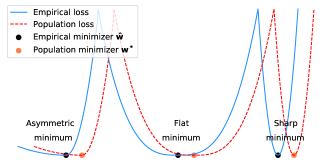
The loss landscape of neural networks has attracted great research interests in the deep learning community (Choromanska et al., 2015; Cooper, 2018; Keskar et al., 2017; Draxler et al., 2018; Ge et al., 2017; Sagun et al., 2017). It provides the basis of designing better optimization algorithms, and helps to answer the question of when and how a deep network can achieve good generalization performance. One hypothesis that draws attention recently is that the local minima of neural networks can be characterized by their flatness, and it is conjectured that sharp minima tend to generalize worse than the flat ones (Keskar et al., 2017). A plausible explanation is that a flat minimizer of the training loss can achieve lower generalization error if the test loss is shifted from the training loss due to random perturbations. Figure 1(a) gives an illustration for this argument.
Refer to caption
(a)
Refer to caption
(b)
Refer to caption
(c)
Figure 1: (a) Three kinds of local minima: asymmetric, flat and sharp. If there exists a shift from empirical loss to population loss, flat minimum is more robust than sharp minimum. (b) For asymmetric valleys, if there exists a random shift, the solution 𝒘~bold-~𝒘\boldsymbol{\tilde{w}} biased towards the flat side is more robust than the minimizer 𝒘^superscriptbold-^𝒘\boldsymbol{\hat{w}^{*}}. (c) SGD tends to stay longer on the flat side of asymmetric valleys, therefore SGD averaging automatically produces the desired bias.

Although being supported by plenty of empirical observations (Keskar et al., 2017; Izmailov et al., 2018; Li et al., 2018), the definition of flatness was recently challenged by (Dinh et al., 2017), who showed that one can construct arbitrarily sharp minima through weight re-parameterization without changing the generalization performance. In addition, recent evidence suggests that the minima of modern deep networks are connected with simple paths with low generalization error (Draxler et al., 2018; Garipov et al., 2018). Similarly, the minima found by large batch training and small batch training are shown to be connected without any “bumps” (Sagun et al., 2017). This raises several questions: (1) If all the minima are well connected, why do some algorithms keep finding sharp minima and others keep finding flat ones (Keskar et al., 2017)? (2) Does flatness really affect generalization?

In this paper, we address these questions by introducing the concept of asymmetric valleys. We observe that the local geometry of the loss function of neural networks is usually asymmetric. In other words, there exist many directions such that the loss increases abruptly along one side, and grows rather slowly along the opposite side (see Figure 1(b) as an illustration). We formally define this kind of local minima as asymmetric valleys. As we will show in Section 6, asymmetric valleys brings interesting illusions in high dimensional space. For example, located in the same valley, 𝒘~bold-~𝒘\boldsymbol{\tilde{w}} may appear to be a wider and flatter minimum than 𝒘^bold-^𝒘\boldsymbol{\hat{w}} as the former is farther away from the sharp side.

For the second question, we argue that flatness does affect generalization. However, we do not simply follow the argument in (Keskar et al., 2017), which states that flat minima tend to generalize better because they are more stable. Instead, we prove that in asymmetric valleys, the solution biased towards the flat side of the valley gives better generalization under mild assumptions. This result has at least two interesting implications: (1) converging to which local minimum (if there are many) may not be critical for modern deep networks. However, it matters a lot where the solution locates; and (2) the solution with lowest a priori generalization error is not necessarily the minimizer of the training loss.

Given that a biased solution is preferred for asymmetric valleys, an immediate question is how we can find such solutions in practice. It turns out that simply averaging the weights along the SGD trajectory, naturally leads to the desired solutions with bias. We give a theoretical analysis to support this argument, see Figure 1(c) for an illustration. Note that our result is in line with the empirical observations recently made by Izmailov et al. (2018).

In addition, we provide empirical analysis to verify our theoretical results and support our claims. For example, we show that asymmetric valleys are indeed prevalent in modern deep networks, and solutions with lower generalization error has bias towards the flat side of the valley. We also find that batch normalization seems to be a major cause for shaping asymmetric loss surfaces.

2 Related Work

Neural network landscape. Analyzing the landscape of deep neural networks is an active and exciting area (Goodfellow & Vinyals, 2014; Li et al., 2018; Ge et al., 2017; Pennington & Bahri, 2017; Wu et al., 2017; Cooper, 2018; Sagun et al., 2017). For example, (Draxler et al., 2018; Garipov et al., 2018) observed that essentially all local minima are connected together with simple paths. (Huang et al., 2017) used cyclic learning rate and took the ensemble of intermediate models to get improved accuracy. There are also appealing visualizations for the neural network landscape (Li et al., 2018).

Sharp and flat minima. The discussion of sharp and flat local minima dates back to (Hochreiter & Schmidhuber, 1995), and recently regains its popularity. For example, Keskar et al. (2017) proposed that large batch SGD finds sharp minima, which leads to poor generalization. In (Chaudhari et al., 2016), an entropy regularized SGD was introduced to explicitly searching for flat minima. It was later pointed out that large batch SGD can yield comparable performance when the learning rate or the number of training iterations are properly set (Hoffer et al., 2017; Goyal et al., 2017; Smith et al., 2017; Masters & Luschi, 2018; Smith & Le, 2017; Jastrzebski et al., 2017). Moreover, (Dinh et al., 2017) showed that from a given flat minimum, one could construct another minimum with arbitrarily sharp directions but equally good performance. In this paper, we argue that the description of sharp or flat minima is an oversimplification. There may simultaneously exist steep directions, flat directions, and asymmetric directions for the same minimum.

SGD optimization and generalization. As the de facto optimization tool for deep networks, SGD and its variants are extensively studied in the literature. For example, it is shown that they could escape saddle points or sharp local minima under reasonable assumptions (Ge et al., 2015; Jin et al., 2017, 2018a, 2018b; Xu et al., 2018; Allen-Zhu, 2018a, b; Allen-Zhu & Li, 2018; Kleinberg et al., 2018). For convex functions (Polyak & Juditsky, 1992) or strongly convex but non-smooth functions (Rakhlin et al., 2012), SGD averaging is shown to give better convergence rate. In addition, it can also achieve higher generalization performance for Lipschitz functions in theory (Shalev-Shwartz et al., 2009; Cesa-bianchi et al., 2002), or for deep networks in practice (Huang et al., 2017; Izmailov et al., 2018; therearemanyconsistentexplanations). Discussions on the generalization bound of neural networks can be found in (Bartlett et al., 2017; Neyshabur et al., 2018, 2017b; Kawaguchi et al., 2017; Neyshabur et al., 2017a; Arora et al., 2018; Zhou et al., 2019).

We show that SGD averaging has implicit bias on the flat sides of the minima. Previously, it was shown that SGD has other kinds of implicit bias as well (Soudry et al., 2017; Ji & Telgarsky, 2018; Gunasekar et al., 2018).

3 Asymmetric Valleys

In this section, we give a formal definition of asymmetric valley, and show that it is prevalent in the loss landscape of modern deep neural networks.

Preliminaries.

In supervised learning, we seek to optimize 𝒘argmin𝒘d𝖫(𝒘),where𝖫(𝒘)𝔼𝒙𝒟[f(𝒙;𝒘)]dformulae-sequencesuperscript𝒘subscriptargmin𝒘superscript𝑑𝖫𝒘where𝖫𝒘subscript𝔼similar-to𝒙𝒟delimited-[]𝑓𝒙𝒘superscript𝑑\boldsymbol{w^{*}}\triangleq\operatorname*{arg\,min}_{\boldsymbol{w}\in\mathbb{R}^{d}}\mathsf{L}(\boldsymbol{w}),~{}~{}\textrm{where}~{}~{}\mathsf{L}(\boldsymbol{w})\triangleq\mathbb{E}_{\boldsymbol{x}\sim\mathcal{D}}[f(\boldsymbol{x};\boldsymbol{w})]\in\mathbb{R}^{d}\rightarrow\mathbb{R} is the population loss, 𝒙m𝒙superscript𝑚\boldsymbol{x}\in\mathbb{R}^{m} is the input from distribution 𝒟𝒟\mathcal{D}, 𝒘d𝒘superscript𝑑\boldsymbol{w}\in\mathbb{R}^{d} denotes the model parameter, and fm×d𝑓superscript𝑚superscript𝑑f\in\mathbb{R}^{m}\times\mathbb{R}^{d}\rightarrow\mathbb{R} is the loss function.

Since the data distribution 𝒟𝒟\mathcal{D} is usually unknown, instead of optimizing 𝖫𝖫\mathsf{L} directly, we often use SGD to find the empirical risk minimizer 𝒘^superscriptbold-^𝒘\boldsymbol{\hat{w}^{*}} for a set of random samples {𝒙i}i=1nsuperscriptsubscriptsubscript𝒙𝑖𝑖1𝑛\{\boldsymbol{x}_{i}\}_{i=1}^{n} from 𝒟𝒟\mathcal{D} (a.k.a. training set): 𝒘^argmin𝒘d𝖫^(𝒘),where𝖫^(𝒘)1ni=1nf(𝒙i;𝒘)formulae-sequencesuperscriptbold-^𝒘subscriptargmin𝒘superscript𝑑^𝖫𝒘where^𝖫𝒘1𝑛superscriptsubscript𝑖1𝑛𝑓subscript𝒙𝑖𝒘\boldsymbol{\hat{w}^{*}}\triangleq\operatorname*{arg\,min}_{\boldsymbol{w}\in\mathbb{R}^{d}}\hat{\mathsf{L}}(\boldsymbol{w}),~{}~{}\mathrm{where}~{}~{}\hat{\mathsf{L}}(\boldsymbol{w})\triangleq\frac{1}{n}\sum_{i=1}^{n}f(\boldsymbol{x}_{i};\boldsymbol{w}).

We use a unit vector 𝒖d𝒖superscript𝑑\boldsymbol{u}\in\mathbb{R}^{d} to represent a direction such that the points on this direction passing 𝒘d𝒘superscript𝑑\boldsymbol{w}\in\mathbb{R}^{d} can be written as 𝒘+l𝒖𝒘𝑙𝒖\boldsymbol{w}+l\boldsymbol{u} for l(,)𝑙l\in(-\infty,\infty).

3.1 Definition of asymmetric valley

Before formally introducing asymmetric valleys, we first define asymmetric directions.

Definition 1 (Asymmetric direction).

Given constants p>0,r>ζ>0,c>1formulae-sequenceformulae-sequence𝑝0𝑟𝜁0𝑐1p>0,r>\zeta>0,c>1, a direction 𝐮𝐮\boldsymbol{u} is (r,p,c,ζ)𝑟𝑝𝑐𝜁(r,p,c,\zeta)-asymmetric with respect to point 𝐰d𝐰superscript𝑑\boldsymbol{w}\in\mathbb{R}^{d} and loss function 𝖫^^𝖫\hat{\mathsf{L}}, if l𝖫^(𝐰+l𝐮)<psubscript𝑙^𝖫𝐰𝑙𝐮𝑝\nabla_{l}\hat{\mathsf{L}}(\boldsymbol{w}+l\boldsymbol{u})<p, and l𝖫^(𝐰l𝐮)<cpsubscript𝑙^𝖫𝐰𝑙𝐮𝑐𝑝\nabla_{l}\hat{\mathsf{L}}(\boldsymbol{w}-l\boldsymbol{u})<-cp for l(ζ,r)𝑙𝜁𝑟l\in(\zeta,r).

To put it simply, asymmetric direction is a direction 𝒖𝒖\boldsymbol{u} along which the loss function grows at different rates at the positive/negative direction. The constant ζ𝜁\zeta handles the small neighborhood around 𝒘𝒘\boldsymbol{w} with very small gradients. With this definition, we now formally define the asymmetric valley.

Definition 2 (Asymmetric valley).

Given constants p,r>ζ>0,c>1formulae-sequence𝑝𝑟𝜁0𝑐1p,r>\zeta>0,c>1, a local minimum 𝐰^superscriptbold-^𝐰\boldsymbol{\hat{w}}^{*} of 𝖫^d^𝖫superscript𝑑\hat{\mathsf{L}}\in\mathbb{R}^{d}\rightarrow\mathbb{R} is a (r,p,c,ζ)𝑟𝑝𝑐𝜁(r,p,c,\zeta)-asymmetric valley, if there exists at least one direction 𝐮𝐮\boldsymbol{u} such that 𝐮𝐮\boldsymbol{u} is (r,p,c,ζ)𝑟𝑝𝑐𝜁(r,p,c,\zeta)-asymmetric with respect to 𝐰^superscriptbold-^𝐰\boldsymbol{\hat{w}^{*}} and 𝖫^^𝖫\hat{\mathsf{L}}.

Notice that here we abuse the name “valley”, since 𝒘^superscriptbold-^𝒘\boldsymbol{\hat{w}^{*}} is essentially a point at the center of a valley.

3.2 Find asymmetric directions empirically
Refer to caption
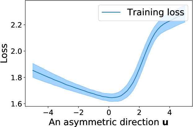
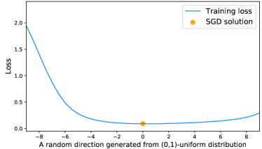
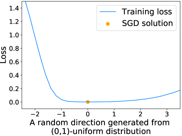
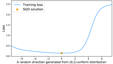
Figure 2: An asymmetric direction of a local minimum on the loss landscape of ResNet-110 trained on CIFAR-10.

Empirically, by taking random directions with value (0,1)01(0,1) in each dimension, we could find an asymmetric direction for a given local minimum with decent probability111By contrast, a random direction with value in (1,1)11(-1,1) is usually not asymmetric. . We perform experiments with three widely used deep networks, i.e., ResNet-110, ResNet-164 (He et al., 2016), DenseNet-100 (Huang et al., 2016), on the CIFAR-10 and CIFAR-100 image classification datasets. For each model on each dataset, we conduct 5 independent runs. The results show that we could always find asymmetric directions with certain specification (r,p,c,ζ)𝑟𝑝𝑐𝜁(r,p,c,\zeta) with c>2𝑐2c>2, which means all the local minima222Notice that empirically we could not verify whether the SGD solution 𝒘^superscriptbold-^𝒘\boldsymbol{\hat{w}^{*}} is a local minimum. See the discussion in Section 6. being found are located in asymmetric valleys. Figure 2 shows an asymmetric direction for a local minimum in ResNet-110 trained on the CIFAR-10 dataset. We verified that it is a (2.5,0.2,7.5,1.2)2.50.27.51.2(2.5,0.2,7.5,1.2)-asymmetric direction. Asymmetric valleys widely exist in other models as well, see Appendix A.

4 Bias and Generalization

As we show in the previous section, most local minima in practice are asymmetric, i.e., they might be sharp on one direction, but flat on the opposite direction. Therefore, it is important to investigate the generalization ability of a solution 𝒘𝒘\boldsymbol{w} in this scenario. In this section, we prove that a biased solution on the flat side of an asymmetric valley yields lower generalization error than the empirical minimizer 𝒘^superscript^𝒘\hat{\boldsymbol{w}}^{*} in that valley.

4.1 Theoretical analysis

Before presenting our theorem, we first introduce two mild assumptions. We will show that they empirically hold on modern deep networks in Section 4.2.

The first assumption (Assumption 1) states that there exists a shift between the empirical loss and true population loss. This is a common assumption in the previous works, e.g., (Keskar et al., 2017), but was usually presented in an informal way. Here we define the “shift” in a formal way. Without loss of generality, we will compare the empirical loss 𝖫^^𝖫\hat{\mathsf{L}} with 𝖫𝖫min𝒘𝖫(𝒘)+min𝒘𝖫^(𝒘)superscript𝖫𝖫subscript𝒘𝖫𝒘subscript𝒘^𝖫𝒘\mathsf{L}^{\prime}\triangleq\mathsf{L}\!-\!\min_{\boldsymbol{w}}\mathsf{L}(\boldsymbol{w})\!+\!\min_{\boldsymbol{w}}\hat{\mathsf{L}}(\boldsymbol{w}) to remove the “vertical difference” between 𝖫^^𝖫\hat{\mathsf{L}} and 𝖫𝖫\mathsf{L}. Notice that min𝒘𝖫(𝒘)subscript𝒘𝖫𝒘\min_{\boldsymbol{w}}\mathsf{L}(\boldsymbol{w}) and min𝒘𝖫^(𝒘)subscript𝒘^𝖫𝒘\min_{\boldsymbol{w}}\hat{\mathsf{L}}(\boldsymbol{w}) are constants and do not affect our generalization guarantee.

Definition 3 ((𝜹,R)𝜹𝑅(\boldsymbol{\delta},R)-shift gap).

For ξ0𝜉0\xi\geq 0, 𝛅d𝛅superscript𝑑\boldsymbol{\delta}\in\mathbb{R}^{d}, and fixed functions 𝖫𝖫\mathsf{L} and 𝖫^^𝖫\hat{\mathsf{L}}, we define the (𝛅,R)𝛅𝑅(\boldsymbol{\delta},R)-shift gap between 𝖫𝖫\mathsf{L} and 𝖫^^𝖫\hat{\mathsf{L}} with respect to a point 𝐰𝐰\boldsymbol{w} as

ξ𝜹(𝒘)=max𝒗𝔹(R)|𝖫(𝒘+𝒗+𝜹)𝖫^(𝒘+𝒗)|subscript𝜉𝜹𝒘subscript𝒗𝔹𝑅superscript𝖫𝒘𝒗𝜹^𝖫𝒘𝒗\xi_{\boldsymbol{\delta}}(\boldsymbol{w})=\max_{\boldsymbol{v}\in\mathbb{B}(R)}|\mathsf{L}^{\prime}(\boldsymbol{w}+\boldsymbol{v}+\boldsymbol{\delta})-\hat{\mathsf{L}}(\boldsymbol{w}+\boldsymbol{v})|

where 𝖫(𝐰)𝖫(𝐰)min𝐰𝖫(𝐰)+min𝐰𝖫^(𝐰)superscript𝖫𝐰𝖫𝐰subscript𝐰𝖫𝐰subscript𝐰^𝖫𝐰\mathsf{L}^{\prime}(\boldsymbol{w})\triangleq\mathsf{L}(\boldsymbol{w})-\min_{\boldsymbol{w}}\mathsf{L}(\boldsymbol{w})+\min_{\boldsymbol{w}}\hat{\mathsf{L}}(\boldsymbol{w}), and 𝔹(R)𝔹𝑅\mathbb{B}(R) is the d𝑑d-dimensional ball with radius R𝑅R centered at 𝟎0\boldsymbol{0}.

From the above definition, we know that the two functions match well after the shift 𝜹𝜹\boldsymbol{\delta} if ξ𝜹(𝒘)subscript𝜉𝜹𝒘\xi_{\boldsymbol{\delta}}(\boldsymbol{w}) is very small. For example, ξ𝜹(𝒘)=0subscript𝜉𝜹𝒘0\xi_{\boldsymbol{\delta}}(\boldsymbol{w})=0 means 𝖫𝖫\mathsf{L} is locally identical to 𝖫^^𝖫\hat{\mathsf{L}} after the shift 𝜹𝜹\boldsymbol{\delta}. Since 𝖫^^𝖫\hat{\mathsf{L}} is computed on a set of random samples from 𝒟𝒟\mathcal{D}, the actual shift 𝜹𝜹\boldsymbol{\delta} between 𝖫^^𝖫\hat{\mathsf{L}} and 𝖫𝖫\mathsf{L} is a random variable, ideally with zero expectation.

Assumption 1 (Random shift assumption).

For a given population loss 𝖫𝖫\mathsf{L} and a random empirical loss 𝖫^^𝖫\hat{\mathsf{L}}, constants R>0,rζ>0,ξ0formulae-sequenceformulae-sequence𝑅0𝑟𝜁0𝜉0R>0,r\geq\zeta>0,\xi\geq 0, a vector 𝛅¯dbold-¯𝛅superscript𝑑\boldsymbol{\bar{\delta}}\in\mathbb{R}^{d} with r𝛅¯iζ𝑟subscriptbold-¯𝛅𝑖𝜁r\geq\boldsymbol{\bar{\delta}}_{i}\geq\zeta for all i[d]𝑖delimited-[]𝑑i\in[d], a minimizer 𝐰^superscriptbold-^𝐰\boldsymbol{\hat{w}}^{*}, we assume that there exists a random variable 𝛅d𝛅superscript𝑑\boldsymbol{\delta}\in\mathbb{R}^{d} correlated with 𝖫^^𝖫\hat{\mathsf{L}} such that Pr(𝛅i=𝛅¯i)=Pr(𝛅i=𝛅¯i)=12Prsubscript𝛅𝑖subscriptbold-¯𝛅𝑖Prsubscript𝛅𝑖subscriptbold-¯𝛅𝑖12\Pr(\boldsymbol{\delta}_{i}=\boldsymbol{\bar{\delta}}_{i})=\Pr(\boldsymbol{\delta}_{i}=-\boldsymbol{\bar{\delta}}_{i})=\frac{1}{2} for all i[d]𝑖delimited-[]𝑑i\in[d], and the (𝛅,R)𝛅𝑅(\boldsymbol{\delta},R)-shift gap between 𝖫𝖫\mathsf{L} and 𝖫^^𝖫\hat{\mathsf{L}} with respect to 𝐰^superscriptbold-^𝐰\boldsymbol{\hat{w}}^{*} is bounded by ξ𝜉\xi.

Roughly, the above assumption says that the local landscape of the empirical loss and population loss match well after applying a shift vector 𝜹𝜹\boldsymbol{\delta}, which has equal probability of being positive or negative in each dimension. Therefore, 𝜹𝜹\boldsymbol{\delta} has 2dsuperscript2𝑑2^{d} possible values for a given shift vector 𝜹¯bold-¯𝜹\boldsymbol{\bar{\delta}}, each with probability 2dsuperscript2𝑑2^{-d}. The second assumption stated below can be seen as an extension of Definition 2.

Assumption 2 (Locally asymmetric).

For a given population loss 𝖫^^𝖫\hat{\mathsf{L}}, and a minimizer 𝐰^superscriptbold-^𝐰\boldsymbol{\hat{w}}^{*}, there exist orthogonal directions 𝐮1,,𝐮kdsuperscript𝐮1superscript𝐮𝑘superscript𝑑\boldsymbol{u}^{1},\cdots,\boldsymbol{u}^{k}\in\mathbb{R}^{d} s.t. 𝐮isuperscript𝐮𝑖\boldsymbol{u}^{i} is (r,pi,ci,ζ)𝑟subscript𝑝𝑖subscript𝑐𝑖𝜁(r,p_{i},c_{i},\zeta)-asymmetric with respect to 𝐰^+𝐯𝐯,𝐮i𝐮isuperscriptbold-^𝐰𝐯𝐯superscript𝐮𝑖superscript𝐮𝑖\boldsymbol{\hat{w}}^{*}+\boldsymbol{v}-\langle\boldsymbol{v},\boldsymbol{u}^{i}\rangle\boldsymbol{u}^{i} for all 𝐯𝔹(R)𝐯𝔹superscript𝑅\boldsymbol{v}\in\mathbb{B}(R^{\prime}) and i[k]𝑖delimited-[]𝑘i\in[k].

Assumption 2 states that if 𝒖isuperscript𝒖𝑖\boldsymbol{u}^{i} is an asymmetric direction at 𝒘^superscriptbold-^𝒘\boldsymbol{\hat{w}}^{*}, then the point 𝒘^+𝒗𝒗,𝒖i𝒖isuperscriptbold-^𝒘𝒗𝒗superscript𝒖𝑖superscript𝒖𝑖\boldsymbol{\hat{w}}^{*}\!+\!\boldsymbol{v}\!-\!\langle\boldsymbol{v},\boldsymbol{u}^{i}\rangle\boldsymbol{u}^{i} that deviates from 𝒘^superscriptbold-^𝒘\boldsymbol{\hat{w}}^{*} along the perpendicular direction of 𝒖isuperscript𝒖𝑖\boldsymbol{u}^{i}, is also asymmetric along the direction of 𝒖isuperscript𝒖𝑖\boldsymbol{u}^{i}. In other words, the neighborhood around 𝒘^superscriptbold-^𝒘\boldsymbol{\hat{w}^{*}} is an asymmetric valley.

Under the above assumptions, we are ready to state our theorem, which says the empirical minimizer is not necessarily the optimal solution, while a biased solution leads to better generalization. We defer the proof to Appendix B.

Theorem 1 (Bias leads to better generalization).

For any 𝐥k𝐥superscript𝑘\boldsymbol{l}\in\mathbb{R}^{k}, if Assumption 1 holds for R=𝐥2𝑅subscriptnorm𝐥2R=\|\boldsymbol{l}\|_{2}, Assumption 2 holds for R=𝛅¯2+𝐥2superscript𝑅subscriptnormbold-¯𝛅2subscriptnorm𝐥2R^{\prime}=\|\boldsymbol{\bar{\delta}}\|_{2}+\|\boldsymbol{l}\|_{2}, and 4ξ(ci1)pi<𝐥imax{r𝛅¯i,𝛅¯iζ}4𝜉subscript𝑐𝑖1subscript𝑝𝑖subscript𝐥𝑖𝑟subscriptbold-¯𝛅𝑖subscriptbold-¯𝛅𝑖𝜁\frac{4\xi}{(c_{i}-1)p_{i}}<\boldsymbol{l}_{i}\leq\max\{r-\boldsymbol{\bar{\delta}}_{i},\boldsymbol{\bar{\delta}}_{i}-\zeta\}, then we have

𝔼𝜹𝖫(𝒘^)𝔼𝜹𝖫(𝒘^+i=1k𝒍i𝒖i)subscript𝔼𝜹𝖫superscriptbold-^𝒘subscript𝔼𝜹𝖫superscriptbold-^𝒘superscriptsubscript𝑖1𝑘subscript𝒍𝑖superscript𝒖𝑖\displaystyle\mathbb{E}_{\boldsymbol{\delta}}\mathsf{L}(\boldsymbol{\hat{w}}^{*})-\mathbb{E}_{\boldsymbol{\delta}}\mathsf{L}\left(\boldsymbol{\hat{w}}^{*}+\sum_{i=1}^{k}\boldsymbol{l}_{i}\boldsymbol{u}^{i}\right)
\displaystyle\geq i=1k(ci1)𝒍ipi/22kξ>0superscriptsubscript𝑖1𝑘subscript𝑐𝑖1subscript𝒍𝑖subscript𝑝𝑖22𝑘𝜉0\displaystyle\sum_{i=1}^{k}(c_{i}-1)\boldsymbol{l}_{i}p_{i}/2-2k\xi>0

Remark on Theorem 1.

It is widely known that the empirical minimizer is usually different from the true optimum. However, in practice it is difficult to know how the training loss shifts from the population loss. Therefore, the best we could do is minimizing the empirical loss function (with some regularizers). On the contrary, Theorem 1 states that under the asymmetric case, we should pick a biased solution to minimize the expected population loss even the shift is unknown. Moreover, it is possible to distill our insight into practical algorithms, as we will discuss in Section 5.

4.2 Verification of assumptions

Verification of Assumption 1.

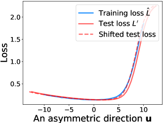
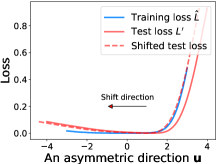
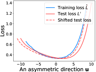
We show that a shift between 𝖫𝖫\mathsf{L} and 𝖫^^𝖫\hat{\mathsf{L}} is quite common in practice, by taking a ResNet-110 trained on CIFAR-10 as an example. Since we could not visualize a shift in a high dimensional space, we randomly sample an asymmetric direction 𝒖𝒖\boldsymbol{u} (more results are shown Appendix C) at the SGD solution 𝒘^superscriptbold-^𝒘\boldsymbol{\hat{w}}^{*}. The blue and red curves shown in Figure 3(a) are obtained by calculating 𝖫^(𝒘^+l𝒖)^𝖫superscriptbold-^𝒘𝑙𝒖\hat{\mathsf{L}}(\boldsymbol{\hat{w}}^{*}+l\boldsymbol{u}) and 𝖫(𝒘^+l𝒖)superscript𝖫superscriptbold-^𝒘𝑙𝒖\mathsf{L}^{\prime}(\boldsymbol{\hat{w}}^{*}+l\boldsymbol{u}) for l[3,3]𝑙33l\in[-3,3], which correspond to the training and test loss, respectively.

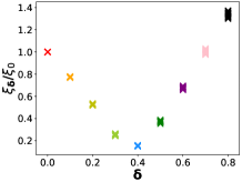
We then try different shift values of 𝜹𝜹\boldsymbol{\delta} to “match” the two curves. As shown in Figure 3(a), after applying a horizontal shift 𝜹=0.4𝜹0.4\boldsymbol{\delta}\!=\!0.4 to the test loss, the two curves overlap almost perfectly. Quantitatively, we can use the shift gap defined in Definition 3 to evaluate how well the two curves match each other after shifting. It turns out that ξ𝜹=0.4=0.0335subscript𝜉𝜹0.40.0335\xi_{\boldsymbol{\delta}=0.4}\!=\!0.0335, which is much lower than ξ𝜹=0=0.223subscript𝜉𝜹00.223\xi_{\boldsymbol{\delta}=0}\!=\!0.223 before shifting (𝜹𝜹\boldsymbol{\delta} has only one dimension here). In Figure 3(b), we plot ξ𝜹/ξ𝟎subscript𝜉𝜹subscript𝜉0\xi_{\boldsymbol{\delta}}/\xi_{\boldsymbol{0}} as a function of 𝜹𝜹\boldsymbol{\delta}. Clearly, there exists a 𝜹𝜹\boldsymbol{\delta} that minimizes this ratio, indicating a good match.

We conducted the same experiments for different directions, models and datasets, and similar observations were made. Please refer to Appendix C for more results.
Refer to caption
(a) Shfit between 𝖫superscript𝖫\mathsf{L}^{\prime} and 𝖫^^𝖫\hat{\mathsf{L}}
Refer to caption
(b) ξ𝜹/ξ𝟎subscript𝜉𝜹subscript𝜉0\xi_{\boldsymbol{\delta}}/\xi_{\boldsymbol{0}} vs different shift 𝜹𝜹\boldsymbol{\delta}
Figure 3: Shift exists between empirical loss and population loss for ResNet-110 on CIFAR-10.

Verification of Assumption 2.

Refer to caption
Figure 4: Training loss mean and standard variance for the neighborhood of 𝒘^superscriptbold-^𝒘\boldsymbol{\hat{w}^{*}} at the direction of 𝒖𝒖\boldsymbol{u}.

This is a mild assumption that can be verified empirically. For example, we take a SGD solution of ResNet-110 on CIFAR-10 as 𝒘^superscriptbold-^𝒘\boldsymbol{\hat{w}}^{*}, and specify an asymmetric direction 𝒖𝒖\boldsymbol{u} for 𝒘^superscriptbold-^𝒘\boldsymbol{\hat{w}^{*}}. We then randomly sample 100100100 different local adjustments for 𝒗𝔹(25)𝒗𝔹25\boldsymbol{v}\in\mathbb{B}(25). Based on these adjustments, we present the mean loss curves and standard variance zone on the asymmetric direction 𝒖𝒖\boldsymbol{u} for all the points 𝒘^+𝒗𝒗,𝒖𝒖superscriptbold-^𝒘𝒗𝒗𝒖𝒖\boldsymbol{\hat{w}^{*}}+\boldsymbol{v}-\langle\boldsymbol{v},\boldsymbol{u}\rangle\boldsymbol{u} in Figure 4. As we can see, the variance of these curves are very small, which means all of them are similar to each other. Moreover, we verified that 𝒖𝒖\boldsymbol{u} is (4,0.1,5.22,2)40.15.222(4,0.1,5.22,2)-asymmetric with respect to all neighboring points.

5 Averaging Generates Good Bias

In the previous section, we show that when the loss landscape of a local minimum is asymmetric, a solution with bias towards the flat side of the valley has better generalization performance. One immediate question is that how can we obtain such a solution via practical algorithms? Below we show that it can be achieved by simply taking the average of SGD iterates during the course of training. We first analyze the one dimensional case in Section 5.1, and then extend the analysis to the high dimensional case in Section 5.2.

5.1 One dimensional case

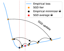
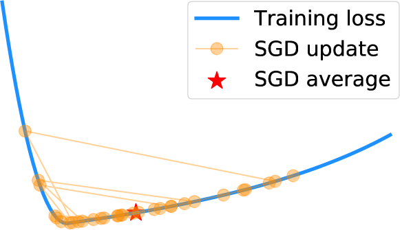
For asymmetric functions, as long as the learning rate is not too small, SGD will oscillate between the flat side and the sharp side. Below we focus on one round of oscillation, and show that the average of the iterates in each round has a bias on the flat side. Consequently, by aggregating all rounds of oscillation, averaging SGD iterates leads to a bias as well.

For each individual round i𝑖i, we assume that it starts from the iteration when SGD goes from sharp side to flat side (denoted as w0isubscriptsuperscript𝑤𝑖0w^{i}_{0}), and ends at the iteration exactly before the iteration that SGD goes from sharp side to flat side again (denoted as wTiisubscriptsuperscript𝑤𝑖subscript𝑇𝑖w^{i}_{T_{i}}). Here Tisubscript𝑇𝑖T_{i} denotes the number of iterations in the i𝑖i-th rounds. The average iterate in the i𝑖i-th round can be written as w¯1Tij=0Tiwji¯𝑤1subscript𝑇𝑖superscriptsubscript𝑗0subscript𝑇𝑖subscriptsuperscript𝑤𝑖𝑗\bar{w}\triangleq\frac{1}{T_{i}}\sum_{j=0}^{T_{i}}w^{i}_{j}. For notational simplicity, we will omit the super script i𝑖i on wjisubscriptsuperscript𝑤𝑖𝑗w^{i}_{j}.

The following theorem shows that the expectation of the average has bias on the flat side. To get a formal lower bound on w¯¯𝑤\bar{w}, we consider the asymmetric case where ζ=0𝜁0\zeta=0, and also assume lower bounds for the gradients on the function. Notice that we made little effort to optimize the constants or bounds on the parameters, and we defer the proof to Appendix E.

Theorem 2 (SGD averaging generates a bias).

Assume that a local minimizer w=0superscript𝑤0w^{*}=0 is a (r,a+,c,0)𝑟subscript𝑎𝑐0(r,a_{+},c,0)-asymmetric valley, where b𝖫(w)a<0subscript𝑏𝖫𝑤subscript𝑎0b_{-}\leq\nabla\mathsf{L}(w)\leq a_{-}<0 for w<0𝑤0w<0, and 0<b+𝖫(w)a+0subscript𝑏𝖫𝑤subscript𝑎0<b_{+}\leq\nabla\mathsf{L}(w)\leq a_{+} for w0𝑤0w\geq 0. Assume a=ca+subscript𝑎𝑐subscript𝑎-a_{-}=ca_{+} for a large constant c𝑐c, and (bν)b+=c<ec/36subscript𝑏𝜈subscript𝑏superscript𝑐superscript𝑒𝑐36\frac{-(b_{-}-\nu)}{b_{+}}=c^{\prime}<\frac{e^{c/3}}{6}. The SGD updating rule is wt+1=wtη(L(w)+ωt)subscript𝑤𝑡1subscript𝑤𝑡𝜂𝐿𝑤subscript𝜔𝑡w_{t+1}=w_{t}-\eta(\nabla L(w)+\omega_{t}) where ωtsubscript𝜔𝑡\omega_{t} is the noise and |ωt|<νsubscript𝜔𝑡𝜈|\omega_{t}|<\nu, and assume νa+𝜈subscript𝑎\nu\leq a_{+}. Then we have

𝔼[w¯]>c0>0,𝔼delimited-[]¯𝑤subscript𝑐00\displaystyle\vspace{-1ex}\mathbb{E}[\bar{w}]>c_{0}>0,\vspace{-1ex}

where c0subscript𝑐0c_{0} is a constant that only depends on η,a+,a,b+,b𝜂subscript𝑎subscript𝑎subscript𝑏subscript𝑏\eta,a_{+},a_{-},b_{+},b_{-} and ν𝜈\nu.

Theorem 2 can be intuitively explained by Figure 5. If we run SGD on this one dimensional function, it will stay at the flat side for more iterations as the magnitude of the gradient on this side is much smaller. Therefore, the average of the locations is biased towards the flat side.
Refer to caption
Figure 5: SGD iterates and their average on an asymmetric function: the oscillation case.

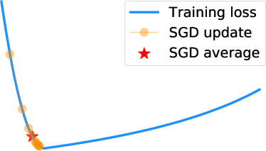
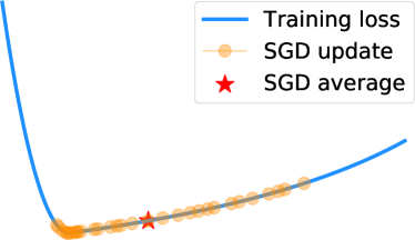
Of course, if the learning rate is sufficiently small, there will be no oscillations on the SGD trajectory, as shown in Figure 6. In this case, the bias on the sharp side tends to be closer to the center compared to the bias on the flat side, as the gradient on the sharp side is much larger than the gradient on the flat side, so SGD converges much faster. In other words, even if there is no oscillation and Theorem 2 does not apply, SGD averaging creates more bias on flat sides than sharp sides in expectation. Thus in all the scenarios, taking average of SGD iterates would be beneficial for asymmetric loss function.

In addition, for symmetric loss functions, averaging SGD iterates may also be helpful in terms of denoising (see Appendix D for concrete examples). Therefore, taking the average of the SGD trajectory may always improve generalization, regardless of whether the loss function is symmetric or not.
Refer to caption
Refer to caption
Figure 6: SGD iterates and their average on an asymmetric function with small learning rate: starting from the sharp side (Left); and starting from the flat side (Right)

5.2 High dimensional case

For high dimensional functions, the analysis on averaging SGD iterates would be more complicated compared to that given in the previous subsection. However, if we only care about the bias on a specific direction 𝒖𝒖\boldsymbol{u}, we could directly apply Theorem 2 with one additional assumption. Specifically, if the projections of the loss function onto 𝒖𝒖\boldsymbol{u} along the SGD trajectory satisfy the assumptions in Theorem 2, i.e., being asymmetric and the gradient on both sides have upper and lower bounds, then the claim of Theorem 2 directly applies. This is because only the gradient along the direction 𝒖𝒖\boldsymbol{u} will affect the SGD trajectory projected onto 𝒖𝒖\boldsymbol{u}, and we could safely omit all other directions.

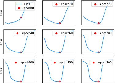
Empirically, we find that this assumption generally holds. For a given SGD solution, we fix a random asymmetric direction 𝒖d𝒖superscript𝑑\boldsymbol{u}\in\mathbb{R}^{d}, and sample the loss surface on direction 𝒖𝒖\boldsymbol{u} that passes the t𝑡t-th epoch of SGD trajectory (denoted as 𝒘𝒕subscript𝒘𝒕\boldsymbol{w_{t}}), i.e., evaluate 𝖫^(𝒘𝒕+l𝒖)^𝖫subscript𝒘𝒕𝑙𝒖\hat{\mathsf{L}}(\boldsymbol{w_{t}}+l\boldsymbol{\boldsymbol{u}}), for 0t2000𝑡2000\leq t\leq 200 and l[15,15]𝑙1515l\in[-15,15].

As shown in the Figure 7, after the first 404040 epochs, the projected loss surfaces becomes relatively stable. Therefore, we could directly apply Theorem 2 to the direction 𝒖𝒖\boldsymbol{u}.

As we will see in Section 6.1, compared with SGD solutions, SGD averaging indeed creates bias along different asymmetric directions, as predicted by our theory.
Refer to caption
Figure 7: Projection of the training loss surface onto an asymmetric direction 𝒖𝒖\boldsymbol{u}

6 Sharp and Flat Minima Illusion

In this section, we show that where the solution locates at a local minimum basin is very important, which is a refinement of judging the generalization performance by the sharpness/flatness of a local minimum. All of our observations support our theoretical analysis in the previous sections.

First we remark that rigorously testing whether a point is a local minimum, or even close to a local minimum, is extremely hard for deep models, see e.g. (Safran & Shamir, 2017). In fact, the Hessian of most empirical solutions still have plenty of small negative eigenvalues (Chaudhari et al., 2016), so technically they are saddle points. But we choose to ignore these technicalities, and treat all these points as “local minima”.

6.1 Illusion case 1: SWA algorithm

Recently, Izmailov et al. (2018) proposed the stochastic weight averaging (SWA) algorithm, which explicitly takes the average of SGD iterates to achieve better generalization. Inspired by their observation that “SWA leads to solutions corresponding to wider optima than SGD”, we provide a more refined explanation in this subsection. That is, averaging weights leads to “biased” solutions in an asymmetric valley, which correspond to better generalization.

Specifically, we run the SWA algorithm (with deceasing learning rate) with three popular deep networks, i.e., ResNet-110, ResNet-164 and DenseNet-100, on the CIFAR-10 and CIFAR-100 datasets, following the configurations in (Izmailov et al., 2018) (denoted as SWA). Then we run SGD with small learning rate from the SWA solutions to find a solution located in the same basin (denoted as SGD).

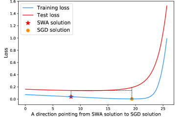
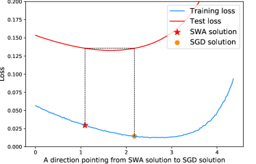
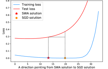
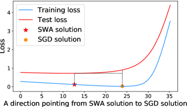
In Figure 8, We draw an interpolation between the solutions obtained by SWA and SGD333Izmailov et al. (2018) have done a similar experiment.. One can observe that there is no “bump” between these two solutions, meaning they are located in the same basin. Clearly, the SWA solution is biased towards the flat side, which verifies our theoretical analysis in Section 5. Further, we notice that although the biased SWA solution has higher training loss than the empirical minimizer, it indeed yields lower test loss. This verifies our analysis in Section 4. Similar observations are made on other networks and other datasets, which we present in Appendix F.
Refer to caption
Figure 8: SWA solution and SGD solution interpolation (ResNet-164 on CIFAR100)

To further support our claim, we list our result in Table 1, from which we can observe that SGD solutions always have higher training accuracy, but worse test accuracy, compared to SWA solutions. This supports our claim in Theorem 1, which states that a bias towards the flat sides of asymmetric valleys could help improve generalization, although it yields higher training error.

Table 1: Training accuracy of various networks on CIFAR-100.
Network CIFAR-100
train test
ResNet-110-SWA 94.98% 78.94%
ResNet-110-SGD 97.52% 78.29%
ResNet-164-SWA 97.48% 80.69%
ResNet-164-SGD 99.12% 76.56%
DenseNet-100-SWA 99.84% 72.29%
DenseNet-100-SGD 99.87% 71.46%

Verifying Theorem 2.

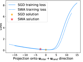
We further verify that averaging SGD solutions could create a bias towards the flat side in expectation for many other asymmetric directions, not just for the specific direction we discussed above.

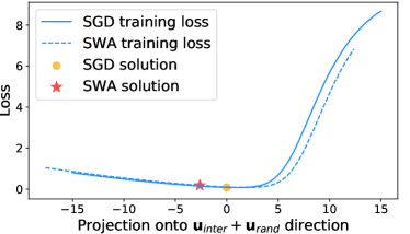
We take a ResNet-110 trained on CIFAR-100 as an example. Denote 𝒖intersubscript𝒖𝑖𝑛𝑡𝑒𝑟\boldsymbol{u}_{inter} as the unit vector pointing from the SGD solution to the SWA solution. We pick another unit random direction 𝒖randsubscript𝒖𝑟𝑎𝑛𝑑\boldsymbol{u}_{rand}. Then, we use the direction 𝒖inter+𝒖randsubscript𝒖𝑖𝑛𝑡𝑒𝑟subscript𝒖𝑟𝑎𝑛𝑑\boldsymbol{u}_{inter}+\boldsymbol{u}_{rand} to verify our claim.

Refer to caption
Figure 9: The average of SGD has a bias on flat side (ResNet-110 on CIFAR100)

The results are shown in Figure 9, from which we can observe that SWA has a bias on the flat side compared with the SGD solution. We create 101010 different random vectors for each network and each dataset, and similar observations can be made (see more examples in Appendix G).

6.2 Illusion case 2: large batch SGD

Keskar et al. (2017) observed that training with small batch size using SGD algorithm generalizes better than training with large batch size. They argue that it is because large batch SGD tends to converge to sharp minima, while small batch SGD generally converges to flat minima. Here we show that it may not be the case in practice.

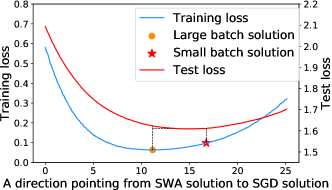
We use a PreResNet-164 trained on CIFAR-100 as an example. We first running SGD with a batch size of 128 for 200 epochs to find a solution (denoted as Large batch solution), and then contintue the training with batch size 32 for another 80 epoch to find a nearby solution (denoted as Small batch solution).

From the results shown in Figure 10, it is clear that the small batch solution has worse training accuracy but better test accuracy. Meanwhile, there is no ’bump’ between these solutions which suggests they are in the same basin. Therefore, small batch SGD generalizes better because it could find a better biased solution in the asymmetric valley, not because it finds a different wider or flatter minimum.
Refer to caption
Figure 10: Large and small minibatch interpolation(batch size 128 to 32 of PreResNet-164 on CIFAR-100)

6.3 Illusion on the width of a minimum

We further point out that visualizing the “width” of a local minimum in a low-dimensional space may lead to illusive results. For example, one visualization technique (Izmailov et al., 2018) is showing how the loss changes along many random directions 𝒗isubscript𝒗𝑖\boldsymbol{v}_{i}’s drawn from the d𝑑d-dimensional Gaussian distribution.

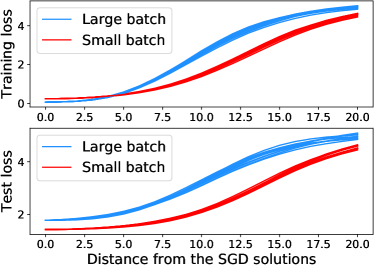
We take the large batch and small batch solutions from the previous subsection as our example. Figure 11 visualizes the “width” of the two solutions using the method described above. From the figure, one may draw the conclusion that small batch training leads to a wider minimum compared to large batch training. However, as discussed in Subsection 6.2 these two solutions are actually from the same basin. In other words, the loss curvature near the two solutions looks different because they are located at different locations in an asymmetric valley, instead of being located at different local minima. Similar observation holds for SWA and SGD solutions, see Appendix H.
Refer to caption
Figure 11: Random ray of large batch and small batch solution(ResNet-164 on CIFAR-100).

7 Batch Norm and Asymmetric Valleys

Preview sections have focused on defining what are asymmetric valleys, and how to leverage them for better generalization. In this section, we take a step forward to answer where they originate, by showing empirical evidences that the Batch Normalization (BN) (Ioffe & Szegedy, 2015) adopted by modern neural networks seems to be a major cause for asymmetric valleys.

Directions on BN parameters are more asymmetric.

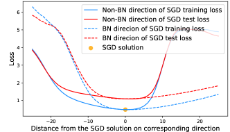
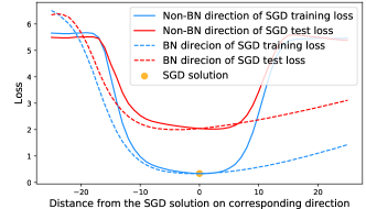
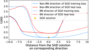
For a given SGD solution, if we take a random direction where only the BN parameters have non-zero entries, and compare it with a random direction where only the non-BN parameters have non-zero entries, we observe that those BN-related directions are usually more asymmetric. The result with ResNet-110 on CIFAR-10 is shown in Figure 12. As we can see, the Non-BN direction is sharp on both sides, but BN direction is flat on one side, and sharp on the other side. We also conducted trials with different networks and datasets, and obtained similar results (see Appendix I).
Refer to caption
Figure 12: BN and Non-BN directions through a local minimum of ResNet-110 on CIFAR-10.

SGD averaging is more effective on BN parameters.

By Theorem 1 and 2, we know that SGD averaging could lead to biased solutions on asymmetric directions with better generalization. If BN indeed creates many asymmetric directions, can we improve the model performance by only averaging the weights of BN layers?

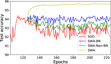
Note that BN parameters only constitute a small fraction of the total model parameters, e.g., 1.41% in a ResNet-110. In the follow experiment on ResNet-110 for CIFAR-10, we perform SGD averaging only on BN parameters, denoted as SWA-BN; and also averaging randomly selected non-BN parameters of the same amount (1.41% of the total parameters), denoted as SWA-Non-BN. The results are shown in Figure 13. It can be observed that averaging only BN parameters (blue curve) is more effective than averaging non-BN parameters (green curve), although there is still a gap comparing to averaging all the weights (yellow curve).
Refer to caption
Figure 13: SGD averaging on BN parameters could give better test accuracy compared with SGD averaging on non-BN parameters.

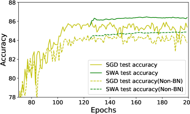
Moreover, we also conduct experiments with two 8-layer ResNets on CIFAR-10, one with BN layers and one without. We choose shallow networks here as deeper models without BN can not be effectively trained.
Refer to caption
Figure 14: Test accuracy of ResNet-8 with and without BN layers, after running weight averaging (SWA).

As shown in figure 14, we start weight averaging at the 126126126-th epoch. Although in both networks, we observe an improvement in test accuracy after averaging, it is clear that the network with BN layers have larger improvement compared with the network without BN layers. This again indicates that SGD averaging is more effective on BN parameters.

The results presented above are still quite preliminary. Understanding how the asymmetric valleys are formed in deep networks might be a valuable future research direction.

8 Conclusion

The width of solutions has been used to explain generalization. In this paper, we elaborate on these arguments, and show that width along Asymmetric Valleys, where the loss may increase at different rates along two opposition directions, is especially important for explaining generalization. Based on a formal definition of asymmetric valley, we showed that a biased solution lying on the flat side of the valley generalizes better than the empirical minimizer. Further, it is proved that by averaging the points along the SGD trajectory naturally leads to such biased solution. We have conducted extensive experiments with state-of-the-art deep models to verify our theorems. We hope this paper will strengthen our understanding on the loss landscape of deep neural networks, and inspire new theories and algorithms that further improve generalization.

References

  • Allen-Zhu (2018a) Allen-Zhu, Z. How to make the gradients small stochastically. CoRR, abs/1801.02982, 2018a.
  • Allen-Zhu (2018b) Allen-Zhu, Z. Natasha 2: Faster non-convex optimization than sgd. In Advances in Neural Information Processing Systems 31, pp. 2680–2691, 2018b.
  • Allen-Zhu & Li (2018) Allen-Zhu, Z. and Li, Y. Neon2: Finding local minima via first-order oracles. In Advances in Neural Information Processing Systems 31, pp. 3720–3730, 2018.
  • Arora et al. (2018) Arora, S., Ge, R., Neyshabur, B., and Zhang, Y. Stronger generalization bounds for deep nets via a compression approach. arXiv preprint arXiv:1802.05296, 2018.
  • Bartlett et al. (2017) Bartlett, P. L., Foster, D. J., and Telgarsky, M. Spectrally-normalized margin bounds for neural networks. CoRR, abs/1706.08498, 2017.
  • Cesa-bianchi et al. (2002) Cesa-bianchi, N., Conconi, A., and Gentile, C. On the generalization ability of on-line learning algorithms. In Advances in Neural Information Processing Systems 14, pp. 359–366. MIT Press, 2002.
  • Chaudhari et al. (2016) Chaudhari, P., Choromanska, A., Soatto, S., LeCun, Y., Baldassi, C., Borgs, C., Chayes, J., Sagun, L., and Zecchina, R. Entropy-SGD: Biasing Gradient Descent Into Wide Valleys. ArXiv e-prints, November 2016.
  • Choromanska et al. (2015) Choromanska, A., LeCun, Y., and Arous, G. B. Open problem: The landscape of the loss surfaces of multilayer networks. In Proceedings of The 28th Conference on Learning Theory, COLT 2015, Paris, France, July 3-6, 2015, pp.  1756–1760, 2015.
  • Cooper (2018) Cooper, Y. The loss landscape of overparameterized neural networks. CoRR, abs/1804.10200, 2018.
  • Dinh et al. (2017) Dinh, L., Pascanu, R., Bengio, S., and Bengio, Y. Sharp Minima Can Generalize For Deep Nets. ArXiv e-prints, March 2017.
  • Draxler et al. (2018) Draxler, F., Veschgini, K., Salmhofer, M., and Hamprecht, F. Essentially no barriers in neural network energy landscape. In Dy, J. and Krause, A. (eds.), Proceedings of the 35th International Conference on Machine Learning, volume 80, pp.  1309–1318, 10–15 Jul 2018.
  • Garipov et al. (2018) Garipov, T., Izmailov, P., Podoprikhin, D., Vetrov, D. P., and Wilson, A. G. Loss surfaces, mode connectivity, and fast ensembling of dnns. CoRR, abs/1802.10026, 2018.
  • Ge et al. (2015) Ge, R., Huang, F., Jin, C., and Yuan, Y. Escaping from saddle points - online stochastic gradient for tensor decomposition. In COLT 2015, volume 40, pp.  797–842, 2015.
  • Ge et al. (2017) Ge, R., Lee, J. D., and Ma, T. Learning One-hidden-layer Neural Networks with Landscape Design. ArXiv e-prints, November 2017.
  • Goodfellow & Vinyals (2014) Goodfellow, I. J. and Vinyals, O. Qualitatively characterizing neural network optimization problems. CoRR, abs/1412.6544, 2014.
  • Goyal et al. (2017) Goyal, P., Dollár, P., Girshick, R. B., Noordhuis, P., Wesolowski, L., Kyrola, A., Tulloch, A., Jia, Y., and He, K. Accurate, large minibatch SGD: training imagenet in 1 hour. CoRR, abs/1706.02677, 2017.
  • Gunasekar et al. (2018) Gunasekar, S., Lee, J., Soudry, D., and Srebro, N. Characterizing implicit bias in terms of optimization geometry. In PMLR, volume 80, pp.  1832–1841, 10–15 Jul 2018.
  • He et al. (2016) He, K., Zhang, X., Ren, S., and Sun, J. Deep residual learning for image recognition. In CVPR, pp.  770–778, 2016.
  • Hochreiter & Schmidhuber (1995) Hochreiter, S. and Schmidhuber, J. Simplifying neural nets by discovering flat minima. In Advances in Neural Information Processing Systems 7, pp. 529–536. MIT Press, 1995.
  • Hoffer et al. (2017) Hoffer, E., Hubara, I., and Soudry, D. Train longer, generalize better: closing the generalization gap in large batch training of neural networks. In Advances in Neural Information Processing Systems 30, pp. 1729–1739. Curran Associates, Inc., 2017.
  • Huang et al. (2016) Huang, G., Liu, Z., Weinberger, K. Q., and van der Maaten, L. Densely Connected Convolutional Networks. ArXiv e-prints, August 2016.
  • Huang et al. (2017) Huang, G., Li, Y., Pleiss, G., Liu, Z., Hopcroft, J. E., and Weinberger, K. Q. Snapshot ensembles: Train 1, get m for free. In ICLR 2017, 2017.
  • Ioffe & Szegedy (2015) Ioffe, S. and Szegedy, C. Batch normalization: Accelerating deep network training by reducing internal covariate shift. In Proceedings of the 32nd International Conference on Machine Learning, ICML 2015, Lille, France, 6-11 July 2015, pp.  448–456, 2015.
  • Izmailov et al. (2018) Izmailov, P., Podoprikhin, D., Garipov, T., Vetrov, D., and Wilson, A. G. Averaging weights leads to wider optima and better generalization. Uncertainty in Artificial Intelligence (UAI), 2018.
  • Jastrzebski et al. (2017) Jastrzebski, S., Kenton, Z., Arpit, D., Ballas, N., Fischer, A., Bengio, Y., and Storkey, A. J. Three factors influencing minima in SGD. CoRR, abs/1711.04623, 2017.
  • Ji & Telgarsky (2018) Ji, Z. and Telgarsky, M. Risk and parameter convergence of logistic regression. CoRR, abs/1803.07300, 2018.
  • Jin et al. (2017) Jin, C., Ge, R., Netrapalli, P., Kakade, S. M., and Jordan, M. I. How to escape saddle points efficiently. CoRR, abs/1703.00887, 2017.
  • Jin et al. (2018a) Jin, C., Liu, L. T., Ge, R., and Jordan, M. I. On the local minima of the empirical risk. In NeurIPS, pp.  4901–4910, 2018a.
  • Jin et al. (2018b) Jin, C., Netrapalli, P., and Jordan, M. I. Accelerated gradient descent escapes saddle points faster than gradient descent. In Conference On Learning Theory, COLT 2018, Stockholm, Sweden, 6-9 July 2018., pp.  1042–1085, 2018b.
  • Kawaguchi et al. (2017) Kawaguchi, K., Pack Kaelbling, L., and Bengio, Y. Generalization in Deep Learning. ArXiv e-prints, October 2017.
  • Keskar et al. (2017) Keskar, N. S., Mudigere, D., Nocedal, J., Smelyanskiy, M., and Tang, P. T. P. On large-batch training for deep learning: Generalization gap and sharp minima. In ICLR 2017, 2017.
  • Kleinberg et al. (2018) Kleinberg, R., Li, Y., and Yuan, Y. An Alternative View: When Does SGD Escape Local Minima? ArXiv e-prints, February 2018.
  • Li et al. (2018) Li, H., Xu, Z., Taylor, G., Studer, C., and Goldstein, T. Visualizing the loss landscape of neural nets. In Advances in Neural Information Processing Systems 31, pp. 6391–6401. Curran Associates, Inc., 2018.
  • Masters & Luschi (2018) Masters, D. and Luschi, C. Revisiting small batch training for deep neural networks. CoRR, abs/1804.07612, 2018.
  • Neyshabur et al. (2017a) Neyshabur, B., Bhojanapalli, S., McAllester, D., and Srebro, N. A pac-bayesian approach to spectrally-normalized margin bounds for neural networks. CoRR, abs/1707.09564, 2017a.
  • Neyshabur et al. (2017b) Neyshabur, B., Bhojanapalli, S., Mcallester, D., and Srebro, N. Exploring generalization in deep learning. In Advances in Neural Information Processing Systems 30, pp. 5947–5956. Curran Associates, Inc., 2017b.
  • Neyshabur et al. (2018) Neyshabur, B., Li, Z., Bhojanapalli, S., LeCun, Y., and Srebro, N. Towards understanding the role of over-parametrization in generalization of neural networks. CoRR, abs/1805.12076, 2018.
  • Pennington & Bahri (2017) Pennington, J. and Bahri, Y. Geometry of neural network loss surfaces via random matrix theory. In Proceedings of the 34th International Conference on Machine Learning, volume 70, pp.  2798–2806. PMLR, 2017.
  • Polyak & Juditsky (1992) Polyak, B. T. and Juditsky, A. B. Acceleration of stochastic approximation by averaging. SIAM J. Control Optim., 30(4):838–855, July 1992. ISSN 0363-0129.
  • Rakhlin et al. (2012) Rakhlin, A., Shamir, O., and Sridharan, K. Making gradient descent optimal for strongly convex stochastic optimization. In ICML, 2012.
  • Safran & Shamir (2017) Safran, I. and Shamir, O. Spurious Local Minima are Common in Two-Layer ReLU Neural Networks. ArXiv e-prints, December 2017.
  • Sagun et al. (2017) Sagun, L., Evci, U., Güney, V. U., Dauphin, Y., and Bottou, L. Empirical analysis of the hessian of over-parametrized neural networks. CoRR, abs/1706.04454, 2017.
  • Shalev-Shwartz et al. (2009) Shalev-Shwartz, S., Shamir, O., Sridharan, K., and Srebro, N. Stochastic convex optimization. In Proceedings of The 22nd Conference on Learning Theory, 2009.
  • Smith & Le (2017) Smith, S. L. and Le, Q. V. A Bayesian Perspective on Generalization and Stochastic Gradient Descent. ArXiv e-prints, October 2017.
  • Smith et al. (2017) Smith, S. L., Kindermans, P., and Le, Q. V. Don’t decay the learning rate, increase the batch size. CoRR, abs/1711.00489, 2017.
  • Soudry et al. (2017) Soudry, D., Hoffer, E., and Srebro, N. The implicit bias of gradient descent on separable data. arXiv preprint arXiv:1710.10345, 2017.
  • Wu et al. (2017) Wu, L., Zhu, Z., et al. Towards understanding generalization of deep learning: Perspective of loss landscapes. arXiv preprint arXiv:1706.10239, 2017.
  • Xu et al. (2018) Xu, Y., Rong, J., and Yang, T. First-order stochastic algorithms for escaping from saddle points in almost linear time. In Advances in Neural Information Processing Systems 31, pp. 5535–5545. Curran Associates, Inc., 2018.
  • Zhou et al. (2019) Zhou, W., Veitch, V., Austern, M., Adams, R. P., and Orbanz, P. Non-vacuous generalization bounds at the imagenet scale: a PAC-bayesian compression approach. In International Conference on Learning Representations, 2019.

Appendix A Additional Figures for Section 3.2: Asymmetric Directions
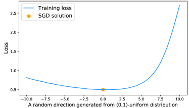
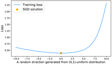
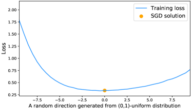
See Figure 15, Figure 16, Figure 17, Figure 18, and Figure 19.

Refer to caption
Figure 15: Asymmetric direction for a solution of ResNet-164 on CIFAR-10. (r,p,c,ζ)=(4.0,0.0270,12.1,2.0)𝑟𝑝𝑐𝜁4.00.027012.12.0(r,p,c,\zeta)=(4.0,0.0270,12.1,2.0).
Refer to caption
Figure 16: Asymmetric direction for a solution of DenseNet-100 on CIFAR-10. (r,p,c,ζ)=(5.0,0.00022,452.5,1.5)𝑟𝑝𝑐𝜁5.00.00022452.51.5(r,p,c,\zeta)=(5.0,0.00022,452.5,1.5).
Refer to caption
Figure 17: Asymmetric direction for a solution of ResNet-110 on CIFAR-100. (r,p,c,ζ)=(8.0,0.032,5.52,4.0)𝑟𝑝𝑐𝜁8.00.0325.524.0(r,p,c,\zeta)=(8.0,0.032,5.52,4.0).
Refer to caption
Figure 18: Asymmetric direction for a solution of ResNet-164 on CIFAR-100. (r,p,c,ζ)=(7.0,0.0175,7.66,3.0)𝑟𝑝𝑐𝜁7.00.01757.663.0(r,p,c,\zeta)=(7.0,0.0175,7.66,3.0).
Refer to caption
Figure 19: Asymmetric direction for a solution of DenseNet-100 on CIFAR-100. (r,p,c,ζ)=(5,0.0198,2.259,2.5)𝑟𝑝𝑐𝜁50.01982.2592.5(r,p,c,\zeta)=(5,0.0198,2.259,2.5).

Appendix B Missing Proof for Theorem 1

Proof.

Since 𝜹𝜹\boldsymbol{\delta} has 2dsuperscript2𝑑2^{d} possible value for a given 𝜹¯¯𝜹\bar{\boldsymbol{\delta}}, we can use an integer j{0,,2d1}𝑗0superscript2𝑑1j\in\{0,\cdots,2^{d}-1\} to represent each value. When writing j𝑗j in binary, its i𝑖i-th digit represents whether 𝜹i=𝜹¯isubscript𝜹𝑖subscriptbold-¯𝜹𝑖{\boldsymbol{\delta}}_{i}=\boldsymbol{\bar{\delta}}_{i} (equal to 111) or 𝜹i=𝜹¯isubscript𝜹𝑖subscriptbold-¯𝜹𝑖{\boldsymbol{\delta}}_{i}=-\boldsymbol{\bar{\delta}}_{i} (equal to 00). We use j2i𝑗superscript2𝑖j\wedge 2^{i} to represent the bitwise AND operator between j𝑗j and 2isuperscript2𝑖2^{i}, which equals 00 if the i𝑖i-th digit of j𝑗j is 00.

To prove our theorem, it suffices to show that for any i[k]𝑖delimited-[]𝑘i\in[k],

𝔼𝜹𝖫(𝒘^+i0=1i1𝒍i0𝒖i0)𝔼𝜹𝖫(𝒘^+i0=1i𝒍i0𝒖i0)(ci1)𝒍ipi/22ξ>0subscript𝔼𝜹𝖫superscriptbold-^𝒘superscriptsubscriptsubscript𝑖01𝑖1subscript𝒍subscript𝑖0subscript𝒖subscript𝑖0subscript𝔼𝜹𝖫superscriptbold-^𝒘superscriptsubscriptsubscript𝑖01𝑖subscript𝒍subscript𝑖0subscript𝒖subscript𝑖0subscript𝑐𝑖1subscript𝒍𝑖subscript𝑝𝑖22𝜉0\displaystyle\mathbb{E}_{\boldsymbol{\delta}}\mathsf{L}\left(\boldsymbol{\hat{w}}^{*}+\sum_{i_{0}=1}^{i-1}\boldsymbol{l}_{i_{0}}\boldsymbol{u}_{i_{0}}\right)-\mathbb{E}_{\boldsymbol{\delta}}\mathsf{L}\left(\boldsymbol{\hat{w}}^{*}+\sum_{i_{0}=1}^{i}\boldsymbol{l}_{i_{0}}\boldsymbol{u}_{i_{0}}\right)\geq(c_{i}-1)\boldsymbol{l}_{i}p_{i}/2-2\xi>0 (1)

If (1) is true, it suffices to take summation over i𝑖i on both sides, and we will get our conclusion. Therefore, below we will prove (1).

𝔼𝜹𝖫(𝒘^+i0=1i1𝒍i0𝒖i0)min𝒘𝖫(𝒘)+min𝒘𝖫^(𝒘)subscript𝔼𝜹𝖫superscriptbold-^𝒘superscriptsubscriptsubscript𝑖01𝑖1subscript𝒍subscript𝑖0subscript𝒖subscript𝑖0subscript𝒘𝖫𝒘subscript𝒘^𝖫𝒘\displaystyle\mathbb{E}_{\boldsymbol{\delta}}\mathsf{L}\left(\boldsymbol{\hat{w}}^{*}+\sum_{i_{0}=1}^{i-1}\boldsymbol{l}_{i_{0}}\boldsymbol{u}_{i_{0}}\right)-\min_{\boldsymbol{w}}\mathsf{L}(\boldsymbol{w})+\min_{\boldsymbol{w}}\hat{\mathsf{L}}(\boldsymbol{w})
=\displaystyle= 𝔼𝜹𝖫(𝒘^+i0=1i1𝒍i0𝒖i0)112dj=02d1𝖫^(𝒘^+i0=1i1𝒍i0𝒖i0+𝜹j)ξsubscript𝔼𝜹superscript𝖫superscriptbold-^𝒘superscriptsubscriptsubscript𝑖01𝑖1subscript𝒍subscript𝑖0subscript𝒖subscript𝑖011superscript2𝑑superscriptsubscript𝑗0superscript2𝑑1^𝖫superscriptbold-^𝒘superscriptsubscriptsubscript𝑖01𝑖1subscript𝒍subscript𝑖0subscript𝒖subscript𝑖0superscript𝜹𝑗𝜉\displaystyle\mathbb{E}_{\boldsymbol{\delta}}\mathsf{L}^{\prime}\left(\boldsymbol{\hat{w}}^{*}+\sum_{i_{0}=1}^{i-1}\boldsymbol{l}_{i_{0}}\boldsymbol{u}_{i_{0}}\right)\overset{\leavevmode\hbox to6.94pt{\vbox to6.94pt{\pgfpicture\makeatletter\hbox{\hskip 3.471pt\lower-3.471pt\hbox to0.0pt{\pgfsys@beginscope\pgfsys@invoke{ }\definecolor{pgfstrokecolor}{rgb}{0,0,0}\pgfsys@color@rgb@stroke{0}{0}{0}\pgfsys@invoke{ }\pgfsys@color@rgb@fill{0}{0}{0}\pgfsys@invoke{ }\pgfsys@setlinewidth{0.4pt}\pgfsys@invoke{ }\nullfont\hbox to0.0pt{\pgfsys@beginscope\pgfsys@invoke{ }{{{}}\hbox{\hbox{{\pgfsys@beginscope\pgfsys@invoke{ }{{}{{{}}}{{}}{}{}{}{}{}{}{}{}{}{{}\pgfsys@moveto{3.271pt}{0.0pt}\pgfsys@curveto{3.271pt}{1.80653pt}{1.80653pt}{3.271pt}{0.0pt}{3.271pt}\pgfsys@curveto{-1.80653pt}{3.271pt}{-3.271pt}{1.80653pt}{-3.271pt}{0.0pt}\pgfsys@curveto{-3.271pt}{-1.80653pt}{-1.80653pt}{-3.271pt}{0.0pt}{-3.271pt}\pgfsys@curveto{1.80653pt}{-3.271pt}{3.271pt}{-1.80653pt}{3.271pt}{0.0pt}\pgfsys@closepath\pgfsys@moveto{0.0pt}{0.0pt}\pgfsys@stroke\pgfsys@invoke{ } }{{{{}}\pgfsys@beginscope\pgfsys@invoke{ }\pgfsys@transformcm{1.0}{0.0}{0.0}{1.0}{-1.75pt}{-2.25555pt}\pgfsys@invoke{ }\hbox{{\definecolor{pgfstrokecolor}{rgb}{0,0,0}\pgfsys@color@rgb@stroke{0}{0}{0}\pgfsys@invoke{ }\pgfsys@color@rgb@fill{0}{0}{0}\pgfsys@invoke{ }\hbox{{\scriptsize 1}} }}\pgfsys@invoke{\lxSVG@closescope }\pgfsys@endscope}}} \pgfsys@invoke{\lxSVG@closescope }\pgfsys@endscope}}} } \pgfsys@invoke{\lxSVG@closescope }\pgfsys@endscope{{{}}}{}{}\hss}\pgfsys@discardpath\pgfsys@invoke{\lxSVG@closescope }\pgfsys@endscope\hss}}\lxSVG@closescope\endpgfpicture}}}{\geq}\frac{1}{2^{d}}\sum_{j=0}^{2^{d}-1}\hat{\mathsf{L}}\left(\boldsymbol{\hat{w}}^{*}+\sum_{i_{0}=1}^{i-1}\boldsymbol{l}_{i_{0}}\boldsymbol{u}_{i_{0}}+\boldsymbol{\delta}^{j}\right)-\xi
=\displaystyle= 12dj=0j2i=02d1[𝖫^(𝒘^+i0=1i1𝒍i0𝒖i0+𝜹j)+𝖫^(𝒘^+i0=1i1𝒍i0𝒖i0+𝜹j+2i)]ξ1superscript2𝑑superscriptsubscript𝑗0𝑗superscript2𝑖0superscript2𝑑1delimited-[]^𝖫superscriptbold-^𝒘superscriptsubscriptsubscript𝑖01𝑖1subscript𝒍subscript𝑖0subscript𝒖subscript𝑖0superscript𝜹𝑗^𝖫superscriptbold-^𝒘superscriptsubscriptsubscript𝑖01𝑖1subscript𝒍subscript𝑖0subscript𝒖subscript𝑖0superscript𝜹𝑗superscript2𝑖𝜉\displaystyle\frac{1}{2^{d}}\sum_{\begin{subarray}{c}j=0\\ j\wedge 2^{i}=0\end{subarray}}^{2^{d}-1}\left[\hat{\mathsf{L}}\left(\boldsymbol{\hat{w}}^{*}+\sum_{i_{0}=1}^{i-1}\boldsymbol{l}_{i_{0}}\boldsymbol{u}_{i_{0}}+\boldsymbol{\delta}^{j}\right)+\hat{\mathsf{L}}\left(\boldsymbol{\hat{w}}^{*}+\sum_{i_{0}=1}^{i-1}\boldsymbol{l}_{i_{0}}\boldsymbol{u}_{i_{0}}+\boldsymbol{\delta}^{j+2^{i}}\right)\right]-\xi (2)

Where 1 holds by Assumption 1, and the fact that i0=1i1𝒍i0𝒖i02𝒍2=Rsubscriptnormsuperscriptsubscriptsubscript𝑖01𝑖1subscript𝒍subscript𝑖0subscript𝒖subscript𝑖02subscriptnorm𝒍2𝑅\|\sum_{i_{0}=1}^{i-1}\boldsymbol{l}_{i_{0}}\boldsymbol{u}_{i_{0}}\|_{2}\leq\|\boldsymbol{l}\|_{2}=R. For every j𝑗j s.t. j2i=0𝑗superscript2𝑖0j\wedge 2^{i}=0,

𝒘^+i0=1i𝒍i0𝒖i0+𝜹jsuperscriptbold-^𝒘superscriptsubscriptsubscript𝑖01𝑖subscript𝒍subscript𝑖0subscript𝒖subscript𝑖0superscript𝜹𝑗\displaystyle\boldsymbol{\hat{w}^{*}}+\sum_{i_{0}=1}^{i}\boldsymbol{l}_{i_{0}}\boldsymbol{u}_{i_{0}}+\boldsymbol{\delta}^{j}
=\displaystyle= 𝒘^+i0=1i𝒍i0𝒖i0+𝜹j+𝜹j,𝒖i𝒖i𝜹j,𝒖i𝒖isuperscriptbold-^𝒘superscriptsubscriptsubscript𝑖01𝑖subscript𝒍subscript𝑖0subscript𝒖subscript𝑖0superscript𝜹𝑗superscript𝜹𝑗superscript𝒖𝑖superscript𝒖𝑖superscript𝜹𝑗superscript𝒖𝑖superscript𝒖𝑖\displaystyle\boldsymbol{\hat{w}^{*}}+\sum_{i_{0}=1}^{i}\boldsymbol{l}_{i_{0}}\boldsymbol{u}_{i_{0}}+\boldsymbol{\delta}^{j}+\langle\boldsymbol{\delta}^{j},\boldsymbol{u}^{i}\rangle\boldsymbol{u}^{i}-\langle\boldsymbol{\delta}^{j},\boldsymbol{u}^{i}\rangle\boldsymbol{u}^{i}
=\displaystyle= 𝒘^+i0=1i1𝒍i0𝒖i0+𝜹j𝜹¯i𝒖i𝜹j,𝒖i𝒖i+𝒍i𝒖isuperscriptbold-^𝒘superscriptsubscriptsubscript𝑖01𝑖1subscript𝒍subscript𝑖0subscript𝒖subscript𝑖0superscript𝜹𝑗subscriptbold-¯𝜹𝑖superscript𝒖𝑖superscript𝜹𝑗superscript𝒖𝑖superscript𝒖𝑖subscript𝒍𝑖superscript𝒖𝑖\displaystyle\boldsymbol{\hat{w}^{*}}+\sum_{i_{0}=1}^{i-1}\boldsymbol{l}_{i_{0}}\boldsymbol{u}_{i_{0}}+\boldsymbol{\delta}^{j}-\boldsymbol{\bar{\delta}}_{i}\boldsymbol{u}^{i}-\langle\boldsymbol{\delta}^{j},\boldsymbol{u}^{i}\rangle\boldsymbol{u}^{i}+\boldsymbol{l}_{i}\boldsymbol{u}^{i}
=\displaystyle= 𝒘^+i0=1i1𝒍i0𝒖i0+𝜹j𝜹j,𝒖i𝒖i+(𝒍i𝜹¯i)𝒖isuperscriptbold-^𝒘superscriptsubscriptsubscript𝑖01𝑖1subscript𝒍subscript𝑖0subscript𝒖subscript𝑖0superscript𝜹𝑗superscript𝜹𝑗superscript𝒖𝑖superscript𝒖𝑖subscript𝒍𝑖subscriptbold-¯𝜹𝑖superscript𝒖𝑖\displaystyle\boldsymbol{\hat{w}^{*}}+\sum_{i_{0}=1}^{i-1}\boldsymbol{l}_{i_{0}}\boldsymbol{u}_{i_{0}}+\boldsymbol{\delta}^{j}-\langle\boldsymbol{\delta}^{j},\boldsymbol{u}^{i}\rangle\boldsymbol{u}^{i}+(\boldsymbol{l}_{i}-\boldsymbol{\bar{\delta}}_{i})\boldsymbol{u}^{i}

Since i0=1i1𝒍i0𝒖i02𝒍2subscriptnormsuperscriptsubscriptsubscript𝑖01𝑖1subscript𝒍subscript𝑖0subscript𝒖subscript𝑖02subscriptnorm𝒍2\|\sum_{i_{0}=1}^{i-1}\boldsymbol{l}_{i_{0}}\boldsymbol{u}_{i_{0}}\|_{2}\leq\|\boldsymbol{l}\|_{2}, δj2=𝜹¯2subscriptnormsuperscript𝛿𝑗2subscriptnormbold-¯𝜹2\|\delta^{j}\|_{2}=\|\boldsymbol{\bar{\delta}}\|_{2}, we know that j,i0=1i1𝒍i0𝒖i0+𝜹j𝔹(R)for-all𝑗superscriptsubscriptsubscript𝑖01𝑖1subscript𝒍subscript𝑖0subscript𝒖subscript𝑖0superscript𝜹𝑗𝔹superscript𝑅\forall j,\sum_{i_{0}=1}^{i-1}\boldsymbol{l}_{i_{0}}\boldsymbol{u}_{i_{0}}+\boldsymbol{\delta}^{j}\in\mathbb{B}(R^{\prime}). By Assumption 2, for every i[k]𝑖delimited-[]𝑘i\in[k], 𝒖isuperscript𝒖𝑖\boldsymbol{u}^{i} is asymmetric with respect to 𝒘^+i0=1i1𝒍i0𝒖i0+𝜹j𝜹j,𝒖i𝒖isuperscriptbold-^𝒘superscriptsubscriptsubscript𝑖01𝑖1subscript𝒍subscript𝑖0subscript𝒖subscript𝑖0superscript𝜹𝑗superscript𝜹𝑗superscript𝒖𝑖superscript𝒖𝑖\boldsymbol{\hat{w}^{*}}+\sum_{i_{0}=1}^{i-1}\boldsymbol{l}_{i_{0}}\boldsymbol{u}_{i_{0}}+\boldsymbol{\delta}^{j}-\langle\boldsymbol{\delta}^{j},\boldsymbol{u}^{i}\rangle\boldsymbol{u}^{i}. Since 𝒍i𝜹¯iζsubscript𝒍𝑖subscriptbold-¯𝜹𝑖𝜁\boldsymbol{l}_{i}\leq\boldsymbol{\bar{\delta}}_{i}-\zeta, we have 𝒍i𝜹¯i<ζsubscript𝒍𝑖subscriptbold-¯𝜹𝑖𝜁\boldsymbol{l}_{i}-\boldsymbol{\bar{\delta}}_{i}<-\zeta. By the definition of asymmetric direction, we know

𝖫^(𝒘^+i0=1i1𝒍i0𝒖i0+𝜹j)𝖫^(𝒘^+i0=1i𝒍i0𝒖i0+𝜹j)+ci𝒍ipi^𝖫superscriptbold-^𝒘superscriptsubscriptsubscript𝑖01𝑖1subscript𝒍subscript𝑖0subscript𝒖subscript𝑖0superscript𝜹𝑗^𝖫superscriptbold-^𝒘superscriptsubscriptsubscript𝑖01𝑖subscript𝒍subscript𝑖0subscript𝒖subscript𝑖0superscript𝜹𝑗subscript𝑐𝑖subscript𝒍𝑖subscript𝑝𝑖\displaystyle\hat{\mathsf{L}}\left(\boldsymbol{\hat{w}^{*}}+\sum_{i_{0}=1}^{i-1}\boldsymbol{l}_{i_{0}}\boldsymbol{u}_{i_{0}}+\boldsymbol{\delta}^{j}\right)\geq\hat{\mathsf{L}}\left(\boldsymbol{\hat{w}^{*}}+\sum_{i_{0}=1}^{i}\boldsymbol{l}_{i_{0}}\boldsymbol{u}_{i_{0}}+\boldsymbol{\delta}^{j}\right)+c_{i}\boldsymbol{l}_{i}p_{i} (3)

Similarly,

𝒘^+i0=1i𝒍i0𝒖i0+𝜹j+2isuperscriptbold-^𝒘superscriptsubscriptsubscript𝑖01𝑖subscript𝒍subscript𝑖0subscript𝒖subscript𝑖0superscript𝜹𝑗superscript2𝑖\displaystyle\boldsymbol{\hat{w}^{*}}+\sum_{i_{0}=1}^{i}\boldsymbol{l}_{i_{0}}\boldsymbol{u}_{i_{0}}+\boldsymbol{\delta}^{j+2^{i}}
=\displaystyle= 𝒘^+i0=1i1𝒍i0𝒖i0+𝜹j+2i+𝜹j+2i,𝒖i𝒖i𝜹j+2i,𝒖i𝒖i+𝒍i𝒖isuperscriptbold-^𝒘superscriptsubscriptsubscript𝑖01𝑖1subscript𝒍subscript𝑖0subscript𝒖subscript𝑖0superscript𝜹𝑗superscript2𝑖superscript𝜹𝑗superscript2𝑖superscript𝒖𝑖superscript𝒖𝑖superscript𝜹𝑗superscript2𝑖superscript𝒖𝑖superscript𝒖𝑖subscript𝒍𝑖superscript𝒖𝑖\displaystyle\boldsymbol{\hat{w}^{*}}+\sum_{i_{0}=1}^{i-1}\boldsymbol{l}_{i_{0}}\boldsymbol{u}_{i_{0}}+\boldsymbol{\delta}^{j+2^{i}}+\langle\boldsymbol{\delta}^{j+2^{i}},\boldsymbol{u}^{i}\rangle\boldsymbol{u}^{i}-\langle\boldsymbol{\delta}^{j+2^{i}},\boldsymbol{u}^{i}\rangle\boldsymbol{u}^{i}+\boldsymbol{l}_{i}\boldsymbol{u}^{i}
=\displaystyle= 𝒘^+i0=1i1𝒍i0𝒖i0+𝜹j+2i𝜹j+2i,𝒖i𝒖i+(𝜹¯i+𝒍i)𝒖isuperscriptbold-^𝒘superscriptsubscriptsubscript𝑖01𝑖1subscript𝒍subscript𝑖0subscript𝒖subscript𝑖0superscript𝜹𝑗superscript2𝑖superscript𝜹𝑗superscript2𝑖superscript𝒖𝑖superscript𝒖𝑖subscriptbold-¯𝜹𝑖subscript𝒍𝑖superscript𝒖𝑖\displaystyle\boldsymbol{\hat{w}^{*}}+\sum_{i_{0}=1}^{i-1}\boldsymbol{l}_{i_{0}}\boldsymbol{u}_{i_{0}}+\boldsymbol{\delta}^{j+2^{i}}-\langle\boldsymbol{\delta}^{j+2^{i}},\boldsymbol{u}^{i}\rangle\boldsymbol{u}^{i}+(\boldsymbol{\bar{\delta}}_{i}+\boldsymbol{l}_{i})\boldsymbol{u}^{i}

Since 𝒍ir𝜹¯isubscript𝒍𝑖𝑟subscriptbold-¯𝜹𝑖\boldsymbol{l}_{i}\leq r-\boldsymbol{\bar{\delta}}_{i}, we have 𝜹¯i+𝒍irsubscriptbold-¯𝜹𝑖subscript𝒍𝑖𝑟\boldsymbol{\bar{\delta}}_{i}+\boldsymbol{l}_{i}\leq r. Therefore,

𝖫^(𝒘^+i0=1i1𝒍i0𝒖i0+𝜹j+2i)𝖫^(𝒘^+i0=1i𝒍i0𝒖i0+𝜹j+2i)𝒍ipi^𝖫superscriptbold-^𝒘superscriptsubscriptsubscript𝑖01𝑖1subscript𝒍subscript𝑖0subscript𝒖subscript𝑖0superscript𝜹𝑗superscript2𝑖^𝖫superscriptbold-^𝒘superscriptsubscriptsubscript𝑖01𝑖subscript𝒍subscript𝑖0subscript𝒖subscript𝑖0superscript𝜹𝑗superscript2𝑖subscript𝒍𝑖subscript𝑝𝑖\displaystyle\hat{\mathsf{L}}\left(\boldsymbol{\hat{w}^{*}}+\sum_{i_{0}=1}^{i-1}\boldsymbol{l}_{i_{0}}\boldsymbol{u}_{i_{0}}+\boldsymbol{\delta}^{j+2^{i}}\right)\geq\hat{\mathsf{L}}\left(\boldsymbol{\hat{w}^{*}}+\sum_{i_{0}=1}^{i}\boldsymbol{l}_{i_{0}}\boldsymbol{u}_{i_{0}}+\boldsymbol{\delta}^{j+2^{i}}\right)-\boldsymbol{l}_{i}p_{i} (4)

Combining (3) and (4), we have,

(2)2absent\displaystyle(\ref{eqn:split_into_pairs})\geq 12dj=0j2i=02d1[𝖫^(𝒘^+i0=1i𝒍i0𝒖i0+𝜹j)+ci𝒍ipi+𝖫^(𝒘^+i0=1i𝒍i0𝒖i0+𝜹j+2i)𝒍ipi]ξ1superscript2𝑑superscriptsubscript𝑗0𝑗superscript2𝑖0superscript2𝑑1delimited-[]^𝖫superscriptbold-^𝒘superscriptsubscriptsubscript𝑖01𝑖subscript𝒍subscript𝑖0subscript𝒖subscript𝑖0superscript𝜹𝑗subscript𝑐𝑖subscript𝒍𝑖subscript𝑝𝑖^𝖫superscriptbold-^𝒘superscriptsubscriptsubscript𝑖01𝑖subscript𝒍subscript𝑖0subscript𝒖subscript𝑖0superscript𝜹𝑗superscript2𝑖subscript𝒍𝑖subscript𝑝𝑖𝜉\displaystyle\frac{1}{2^{d}}\sum_{\begin{subarray}{c}j=0\\ j\wedge 2^{i}=0\end{subarray}}^{2^{d}-1}\left[\hat{\mathsf{L}}\left(\boldsymbol{\hat{w}}^{*}+\sum_{i_{0}=1}^{i}\boldsymbol{l}_{i_{0}}\boldsymbol{u}_{i_{0}}+\boldsymbol{\delta}^{j}\right)+c_{i}\boldsymbol{l}_{i}p_{i}+\hat{\mathsf{L}}\left(\boldsymbol{\hat{w}}^{*}+\sum_{i_{0}=1}^{i}\boldsymbol{l}_{i_{0}}\boldsymbol{u}_{i_{0}}+\boldsymbol{\delta}^{j+2^{i}}\right)-\boldsymbol{l}_{i}p_{i}\right]-\xi
=\displaystyle= 12dj=02d1[𝖫^(𝒘^+i0=1i𝒍i𝒖i0+𝜹j)]+(ci1)𝒍ipi/2ξ1superscript2𝑑superscriptsubscript𝑗0superscript2𝑑1delimited-[]^𝖫superscriptbold-^𝒘superscriptsubscriptsubscript𝑖01𝑖subscript𝒍𝑖subscript𝒖subscript𝑖0superscript𝜹𝑗subscript𝑐𝑖1subscript𝒍𝑖subscript𝑝𝑖2𝜉\displaystyle\frac{1}{2^{d}}\sum_{j=0}^{2^{d}-1}\left[\hat{\mathsf{L}}\left(\boldsymbol{\hat{w}}^{*}+\sum_{i_{0}=1}^{i}\boldsymbol{l}_{i}\boldsymbol{u}_{i_{0}}+\boldsymbol{\delta}^{j}\right)\right]+(c_{i}-1)\boldsymbol{l}_{i}p_{i}/2-\xi
22\displaystyle\overset{\leavevmode\hbox to6.94pt{\vbox to6.94pt{\pgfpicture\makeatletter\hbox{\hskip 3.471pt\lower-3.471pt\hbox to0.0pt{\pgfsys@beginscope\pgfsys@invoke{ }\definecolor{pgfstrokecolor}{rgb}{0,0,0}\pgfsys@color@rgb@stroke{0}{0}{0}\pgfsys@invoke{ }\pgfsys@color@rgb@fill{0}{0}{0}\pgfsys@invoke{ }\pgfsys@setlinewidth{0.4pt}\pgfsys@invoke{ }\nullfont\hbox to0.0pt{\pgfsys@beginscope\pgfsys@invoke{ }{{{}}\hbox{\hbox{{\pgfsys@beginscope\pgfsys@invoke{ }{{}{{{}}}{{}}{}{}{}{}{}{}{}{}{}{{}\pgfsys@moveto{3.271pt}{0.0pt}\pgfsys@curveto{3.271pt}{1.80653pt}{1.80653pt}{3.271pt}{0.0pt}{3.271pt}\pgfsys@curveto{-1.80653pt}{3.271pt}{-3.271pt}{1.80653pt}{-3.271pt}{0.0pt}\pgfsys@curveto{-3.271pt}{-1.80653pt}{-1.80653pt}{-3.271pt}{0.0pt}{-3.271pt}\pgfsys@curveto{1.80653pt}{-3.271pt}{3.271pt}{-1.80653pt}{3.271pt}{0.0pt}\pgfsys@closepath\pgfsys@moveto{0.0pt}{0.0pt}\pgfsys@stroke\pgfsys@invoke{ } }{{{{}}\pgfsys@beginscope\pgfsys@invoke{ }\pgfsys@transformcm{1.0}{0.0}{0.0}{1.0}{-1.75pt}{-2.25555pt}\pgfsys@invoke{ }\hbox{{\definecolor{pgfstrokecolor}{rgb}{0,0,0}\pgfsys@color@rgb@stroke{0}{0}{0}\pgfsys@invoke{ }\pgfsys@color@rgb@fill{0}{0}{0}\pgfsys@invoke{ }\hbox{{\scriptsize 2}} }}\pgfsys@invoke{\lxSVG@closescope }\pgfsys@endscope}}} \pgfsys@invoke{\lxSVG@closescope }\pgfsys@endscope}}} } \pgfsys@invoke{\lxSVG@closescope }\pgfsys@endscope{{{}}}{}{}\hss}\pgfsys@discardpath\pgfsys@invoke{\lxSVG@closescope }\pgfsys@endscope\hss}}\lxSVG@closescope\endpgfpicture}}}{\geq} 𝔼𝜹𝖫(𝒘^+i0=1i𝒍i0𝒖i0)+(ci1)𝒍ipi/22ξsubscript𝔼𝜹superscript𝖫superscriptbold-^𝒘superscriptsubscriptsubscript𝑖01𝑖subscript𝒍subscript𝑖0subscript𝒖subscript𝑖0subscript𝑐𝑖1subscript𝒍𝑖subscript𝑝𝑖22𝜉\displaystyle\mathbb{E}_{\boldsymbol{\delta}}\mathsf{L}^{\prime}\left(\boldsymbol{\hat{w}}^{*}+\sum_{i_{0}=1}^{i}\boldsymbol{l}_{i_{0}}\boldsymbol{u}_{i_{0}}\right)+(c_{i}-1)\boldsymbol{l}_{i}p_{i}/2-2\xi
=\displaystyle= 𝔼𝜹𝖫(𝒘^+i0=1i𝒍i0𝒖i0)min𝒘𝖫(𝒘)+min𝒘𝖫^(𝒘)+(ci1)𝒍ipi/22ξsubscript𝔼𝜹𝖫superscriptbold-^𝒘superscriptsubscriptsubscript𝑖01𝑖subscript𝒍subscript𝑖0subscript𝒖subscript𝑖0subscript𝒘𝖫𝒘subscript𝒘^𝖫𝒘subscript𝑐𝑖1subscript𝒍𝑖subscript𝑝𝑖22𝜉\displaystyle\mathbb{E}_{\boldsymbol{\delta}}\mathsf{L}\left(\boldsymbol{\hat{w}}^{*}+\sum_{i_{0}=1}^{i}\boldsymbol{l}_{i_{0}}\boldsymbol{u}_{i_{0}}\right)-\min_{\boldsymbol{w}}\mathsf{L}(\boldsymbol{w})+\min_{\boldsymbol{w}}\hat{\mathsf{L}}(\boldsymbol{w})+(c_{i}-1)\boldsymbol{l}_{i}p_{i}/2-2\xi

Where 2 holds by Assumption 1 and the fact that i0=1i𝒍i0𝒖i02𝒍2=Rsubscriptnormsuperscriptsubscriptsubscript𝑖01𝑖subscript𝒍subscript𝑖0subscript𝒖subscript𝑖02subscriptnorm𝒍2𝑅\|\sum_{i_{0}=1}^{i}\boldsymbol{l}_{i_{0}}\boldsymbol{u}_{i_{0}}\|_{2}\leq\|\boldsymbol{l}\|_{2}=R. That means,

𝔼𝜹𝖫(𝒘^+i0=1i1𝒍i0𝒖i0)𝔼𝜹𝖫(𝒘^+i0=1i𝒍i0𝒖i0)+(ci1)𝒍ipi/22ξ>0subscript𝔼𝜹𝖫superscriptbold-^𝒘superscriptsubscriptsubscript𝑖01𝑖1subscript𝒍subscript𝑖0subscript𝒖subscript𝑖0subscript𝔼𝜹𝖫superscriptbold-^𝒘superscriptsubscriptsubscript𝑖01𝑖subscript𝒍subscript𝑖0subscript𝒖subscript𝑖0subscript𝑐𝑖1subscript𝒍𝑖subscript𝑝𝑖22𝜉0\displaystyle\mathbb{E}_{\boldsymbol{\delta}}\mathsf{L}\left(\boldsymbol{\hat{w}}^{*}+\sum_{i_{0}=1}^{i-1}\boldsymbol{l}_{i_{0}}\boldsymbol{u}_{i_{0}}\right)\geq\mathbb{E}_{\boldsymbol{\delta}}\mathsf{L}\left(\boldsymbol{\hat{w}}^{*}+\sum_{i_{0}=1}^{i}\boldsymbol{l}_{i_{0}}\boldsymbol{u}_{i_{0}}\right)+(c_{i}-1)\boldsymbol{l}_{i}p_{i}/2-2\xi>0

Where the last inequality holds as 𝒍i>4ξ(ci1)pisubscript𝒍𝑖4𝜉subscript𝑐𝑖1subscript𝑝𝑖\boldsymbol{l}_{i}>\frac{4\xi}{(c_{i}-1)p_{i}}.

Appendix C Additional Figures for Section 4.2: Shift Exists Empirically
See Figure 20, Figure 21, and Figure 22.

Refer to caption
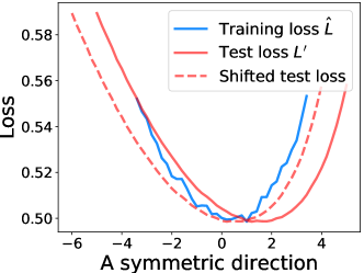
Figure 20: Shift on asymmetric direction (DenseNet-100 on CIFAR-100), ξ𝜹=1=0.119subscript𝜉𝜹10.119\xi_{\boldsymbol{\delta}=1}\!=\!0.119, ξ𝜹=0=0.439subscript𝜉𝜹00.439\xi_{\boldsymbol{\delta}=0}\!=\!0.439
Refer to caption
Figure 21: Shift on asymmetric direction (ResNet-164 on CIFAR-10), ξ𝜹=0.5=0.0699subscript𝜉𝜹0.50.0699\xi_{\boldsymbol{\delta}=0.5}\!=\!0.0699, ξ𝜹=0=0.189subscript𝜉𝜹00.189\xi_{\boldsymbol{\delta}=0}\!=\!0.189
Refer to caption
Figure 22: Shift on symmetric direction (ResNet-110 on CIFAR-100), ξ𝜹=1=0.0197subscript𝜉𝜹10.0197\xi_{\boldsymbol{\delta}=1}\!=\!0.0197, ξ𝜹=0=0.0431subscript𝜉𝜹00.0431\xi_{\boldsymbol{\delta}=0}\!=\!0.0431

Appendix D Additional Figures in Section 5: Averaging Works For Symmetric Case

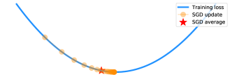
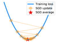
If the function is symmetric, there are two possible cases, as we show in Figure 23 and Figure 24. On one hand, if the function is flat, SGD is likely to stay on one side of the function along the trajectory, and the average will have bias on that side. On the other hand, if the function is sharp, SGD is likely to oscillate between the two sides, and therefore the average of the iterates will concentrate around the center. In both cases, SGD averaging could help to create bias on flat sides or to denoise.
Refer to caption
Figure 23: Symmetric function with flat sides
Refer to caption
Figure 24: Symmetric function with sharp sides

Appendix E Missing Proof for Theorem 2

To prove Theorem 2, we will need the following concentration bound.

Lemma 3 (Azuma’s inequality).

Let X1,X2,X3,Xnsubscript𝑋1subscript𝑋2subscript𝑋3subscript𝑋𝑛X_{1},X_{2},X_{3},...X_{n} be independent random variables satisfying |Xi𝔼[Xi]|cisubscript𝑋𝑖𝔼delimited-[]subscript𝑋𝑖subscript𝑐𝑖|X_{i}-\mathbb{E}[X_{i}]|\leq c_{i}, for 1in1𝑖𝑛1\leq i\leq n. We have the following bound for X=i=1nXi𝑋superscriptsubscript𝑖1𝑛subscript𝑋𝑖X=\sum_{i=1}^{n}X_{i}:

Pr(|X𝔼(X)|λ)2eλ22i=1nci2Pr𝑋𝔼𝑋𝜆2superscript𝑒superscript𝜆22superscriptsubscript𝑖1𝑛superscriptsubscript𝑐𝑖2\Pr(|X-\mathbb{E}(X)|\geq\lambda)\leq 2e^{-\frac{\lambda^{2}}{2\sum_{i=1}^{n}c_{i}^{2}}}

Let pminη(a+a++2ν)subscript𝑝𝜂subscript𝑎subscript𝑎2𝜈p_{\min}\triangleq-\eta(a_{-}+a_{+}+2\nu), pmaxη(bν)subscript𝑝𝜂subscript𝑏𝜈p_{\max}\triangleq-\eta(b_{-}-\nu). Since a=ca+subscript𝑎𝑐subscript𝑎-a_{-}=ca_{+}, we know pmin>(c1)ηa+2ηνsubscript𝑝𝑐1𝜂subscript𝑎2𝜂𝜈p_{\min}>(c-1)\eta a_{+}-2\eta\nu. First, we have the following bounds on the first step w0subscript𝑤0w_{0}.

Lemma 4.

For every i[h]𝑖delimited-[]i\in[h], w0[pmin,pmax]subscript𝑤0subscript𝑝subscript𝑝w_{0}\in[p_{\min},p_{\max}].

Proof.

Since w0subscript𝑤0w_{0} is the first step that SGD jumps from the flat side to the sharp side, denote the previous location as w1<0subscript𝑤10w_{-1}<0. Since w1subscript𝑤1w_{-1} is at the sharp side, we know that the gradient is 𝖫(w1)a𝖫subscript𝑤1subscript𝑎\nabla\mathsf{L}(w_{-1})\leq a_{-}. Therefore, we have

w0=w1η(𝖫(w1)+ω1)subscript𝑤0subscript𝑤1𝜂𝖫subscript𝑤1subscript𝜔1w_{0}=w_{-1}-\eta(\nabla\mathsf{L}(w_{-1})+\omega_{-1})

Where ω1subscript𝜔1\omega_{-1} is the noise bounded by ν𝜈\nu.

At the time when SGD jump from the flat side to sharp side, denote the target position as w1subscriptsuperscript𝑤1w^{\prime}_{-1}. We know that w1[η(a++ν),0]subscriptsuperscript𝑤1𝜂subscript𝑎𝜈0w^{\prime}_{-1}\in[-\eta(a_{+}+\nu),0]. Since the gradient on the sharp side is at most asubscript𝑎a_{-}, we know the next step is lower bounded by η(a++2ν+a)=pmin>0𝜂subscript𝑎2𝜈subscript𝑎subscript𝑝0-\eta(a_{+}+2\nu+a_{-})=p_{\min}>0. In other words, SGD stays at the sharp side for only 111 iterations (this matches with our empirical observation, see e.g. Figure 5).

That means, the bound on w1subscriptsuperscript𝑤1w^{\prime}_{-1} can be applied to w1subscript𝑤1w_{-1} as well, because they are the same iterate. By applying the upper and lower bound on 𝖫(w1)𝖫subscript𝑤1\nabla\mathsf{L}(w_{-1}), we get:

w0η(a++ν)η(a+ν)=pminsubscript𝑤0𝜂subscript𝑎𝜈𝜂subscript𝑎𝜈subscript𝑝w_{0}\geq-\eta(a_{+}+\nu)-\eta(a_{-}+\nu)=p_{\min}

and also

w00η(bν)=pmaxsubscript𝑤00𝜂subscript𝑏𝜈subscript𝑝w_{0}\leq 0-\eta(b_{-}-\nu)=p_{\max}

Below we first define Tmin(2νlog1/2(2τ)+2ν2log(2τ)4a+(a+a++2ν)2a+)2subscript𝑇superscript2𝜈superscript122𝜏2superscript𝜈22𝜏4subscript𝑎subscript𝑎subscript𝑎2𝜈2subscript𝑎2T_{\min}\triangleq\left(\frac{-\sqrt{2}\nu\log^{1/2}(2\tau)+\sqrt{2\nu^{2}\log(2\tau)-4a_{+}(a_{-}+a_{+}+2\nu)}}{2a_{+}}\right)^{2}, where τ𝜏\tau is a constant with value to be set later. Tminsubscript𝑇T_{\min} satisfies the following inequality.

Lemma 5.

tTmin,pmintηa+2tηνlog1/2(2τ)0formulae-sequencefor-all𝑡subscript𝑇subscript𝑝𝑡𝜂subscript𝑎2𝑡𝜂𝜈superscript122𝜏0\forall t\leq T_{\min},p_{\min}-t\eta a_{+}-\sqrt{2t}\eta\nu\log^{1/2}(2\tau)\geq 0.

Proof.

By the definition of pminsubscript𝑝p_{\min}, we have

η(a+a++2ν)tηa+2tηνlog1/2(2τ)0𝜂subscript𝑎subscript𝑎2𝜈𝑡𝜂subscript𝑎2𝑡𝜂𝜈superscript122𝜏0\displaystyle-\eta(a_{-}+a_{+}+2\nu)-t\eta a_{+}-\sqrt{2t}\eta\nu\log^{1/2}(2\tau)\geq 0
\displaystyle\Leftarrow (a+a++2ν)+ta++2tνlog1/2(2τ)0subscript𝑎subscript𝑎2𝜈𝑡subscript𝑎2𝑡𝜈superscript122𝜏0\displaystyle(a_{-}+a_{+}+2\nu)+ta_{+}+\sqrt{2t}\nu\log^{1/2}(2\tau)\leq 0
\displaystyle\Leftarrow (a+a++2ν)+Δ2a++2Δrlog1/2(2τ)0(Δt)subscript𝑎subscript𝑎2𝜈superscriptΔ2subscript𝑎2Δ𝑟superscript122𝜏0Δt\displaystyle(a_{-}+a_{+}+2\nu)+\Delta^{2}a_{+}+\sqrt{2}\Delta r\log^{1/2}(2\tau)\leq 0~{}~{}~{}~{}~{}(\mathrm{\Delta\triangleq\sqrt{t}})
\displaystyle\Leftarrow Δ[0,2νlog1/2(2τ)+2ν2log(2τ)4a+(a+a++2ν)2a+]Δ02𝜈superscript122𝜏2superscript𝜈22𝜏4subscript𝑎subscript𝑎subscript𝑎2𝜈2subscript𝑎\displaystyle\Delta\in\left[0,\frac{-\sqrt{2}\nu\log^{1/2}(2\tau)+\sqrt{2\nu^{2}\log(2\tau)-4a_{+}(a_{-}+a_{+}+2\nu)}}{2a_{+}}\right]
\displaystyle\Leftarrow t(2νlog1/2(2τ)+2ν2log(2τ)4a+(a+a++2ν)2a+)2𝑡superscript2𝜈superscript122𝜏2superscript𝜈22𝜏4subscript𝑎subscript𝑎subscript𝑎2𝜈2subscript𝑎2\displaystyle t\leq\left(\frac{-\sqrt{2}\nu\log^{1/2}(2\tau)+\sqrt{2\nu^{2}\log(2\tau)-4a_{+}(a_{-}+a_{+}+2\nu)}}{2a_{+}}\right)^{2}\qed

Now, we have the following theorem that says with decent probability, the minimum number of iterates on the flat side in i𝑖i-th round is at least Tminsubscript𝑇T_{\min}.

Theorem 6.

If we start at w0pminsubscript𝑤0subscript𝑝w_{0}\geq p_{\min}, for every fixed τ>Tmin𝜏subscript𝑇\tau>T_{\min}, with probability at least 1Tminτ1subscript𝑇𝜏1-\frac{T_{\min}}{\tau}, we have tTmin,wt>w0tηa+2tηνlog1/2(2τ)0formulae-sequencefor-all𝑡subscript𝑇subscript𝑤𝑡subscript𝑤0𝑡𝜂subscript𝑎2𝑡𝜂𝜈superscript122𝜏0\forall t\leq T_{\min},w_{t}>w_{0}-t\eta a_{+}-\sqrt{2t}\eta\nu\log^{1/2}(2\tau)\geq 0.

Proof.

Define filtration t=σ{ω0,,ωt1}subscript𝑡𝜎subscript𝜔0subscript𝜔𝑡1\mathcal{F}_{t}=\sigma\{\omega_{0},\cdots,\omega_{t-1}\}, where σ{}𝜎\sigma\{\cdot\} denotes the sigma field. Define the event 𝔈T={tT,wt>w0tηa+2tηνlog1/2(2τ)}subscript𝔈𝑇formulae-sequencefor-all𝑡𝑇subscript𝑤𝑡subscript𝑤0𝑡𝜂subscript𝑎2𝑡𝜂𝜈superscript122𝜏\mathfrak{E}_{T}=\{\forall t\leq T,w_{t}>w_{0}-t\eta a_{+}-\sqrt{2t}\eta\nu\log^{1/2}(2\tau)\} and define Gt=w0wttηa++Msubscript𝐺𝑡subscript𝑤0subscript𝑤𝑡𝑡𝜂subscript𝑎𝑀G_{t}=w_{0}-w_{t}-t\eta a_{+}+M, where M(Tmin+1)(w0+ν+2ηa+)𝑀subscript𝑇1subscript𝑤0𝜈2𝜂subscript𝑎M\triangleq(T_{\min}+1)(w_{0}+\nu+2\eta a_{+}). Since we only consider the case tTmin𝑡subscript𝑇t\leq T_{\min}, we have

Gt=w0wttηa++(Tmin+1)(w0+ν+2ηa+)>w0wttηa++wt+tηa+>0subscript𝐺𝑡subscript𝑤0subscript𝑤𝑡𝑡𝜂subscript𝑎subscript𝑇1subscript𝑤0𝜈2𝜂subscript𝑎subscript𝑤0subscript𝑤𝑡𝑡𝜂subscript𝑎subscript𝑤𝑡𝑡𝜂subscript𝑎0G_{t}=w_{0}-w_{t}-t\eta a_{+}+(T_{\min}+1)(w_{0}+\nu+2\eta a_{+})>w_{0}-w_{t}-t\eta a_{+}+w_{t}+t\eta a_{+}>0

Therefore, Gtsubscript𝐺𝑡G_{t} is always positive. By SGD updating rule, we have

𝔼[Gt+1𝟙𝔈t|t]=𝔼[(w0wt+1(t+1)ηa++M)𝟙𝔈t|t]𝔼delimited-[]conditionalsubscript𝐺𝑡1subscriptdouble-struck-𝟙subscript𝔈𝑡subscript𝑡𝔼delimited-[]conditionalsubscript𝑤0subscript𝑤𝑡1𝑡1𝜂subscript𝑎𝑀subscriptdouble-struck-𝟙subscript𝔈𝑡subscript𝑡\displaystyle\mathbb{E}[G_{t+1}\mathbb{1}_{\mathfrak{E}_{t}}|\mathcal{F}_{t}]=\mathbb{E}[(w_{0}-w_{t+1}-(t+1)\eta a_{+}+M)\mathbb{1}_{\mathfrak{E}_{t}}|\mathcal{F}_{t}]
\displaystyle\leq 𝔼[(w0wt+ηωttηa++M)𝟙𝔈t|t]=w0wttηa++M=Gt𝟙𝔈t𝔼delimited-[]conditionalsubscript𝑤0subscript𝑤𝑡𝜂subscript𝜔𝑡𝑡𝜂subscript𝑎𝑀subscriptdouble-struck-𝟙subscript𝔈𝑡subscript𝑡subscript𝑤0subscript𝑤𝑡𝑡𝜂subscript𝑎𝑀subscript𝐺𝑡subscriptdouble-struck-𝟙subscript𝔈𝑡\displaystyle\mathbb{E}[(w_{0}-w_{t}+\eta\omega_{t}-t\eta a_{+}+M)\mathbb{1}_{\mathfrak{E}_{t}}|\mathcal{F}_{t}]=w_{0}-w_{t}-t\eta a_{+}+M=G_{t}\mathbb{1}_{\mathfrak{E}_{t}} (5)

Since 𝟙𝔈t𝟙𝔈t1subscriptdouble-struck-𝟙subscript𝔈𝑡subscriptdouble-struck-𝟙subscript𝔈𝑡1\mathbb{1}_{\mathfrak{E}_{t}}\leq\mathbb{1}_{\mathfrak{E}_{t-1}}, and Gtsubscript𝐺𝑡G_{t} is always positive, we have

Gt𝟙𝔈tGt𝟙𝔈t1subscript𝐺𝑡subscriptdouble-struck-𝟙subscript𝔈𝑡subscript𝐺𝑡subscriptdouble-struck-𝟙subscript𝔈𝑡1G_{t}\mathbb{1}_{\mathfrak{E}_{t}}\leq G_{t}\mathbb{1}_{\mathfrak{E}_{t-1}} (6)

Combining (5) and (6) together, we know Gt𝟙𝔈t1subscript𝐺𝑡subscriptdouble-struck-𝟙subscript𝔈𝑡1G_{t}\mathbb{1}_{\mathfrak{E}_{t-1}} is a supermartingale.

We can also bound the absolute value of the difference in every iteration:

|Gt+1𝟙𝔈t𝔼[Gt+1𝟙𝔈t|t]|\displaystyle|G_{t+1}\mathbb{1}_{\mathfrak{E}_{t}}-\mathbb{E}[G_{t+1}\mathbb{1}_{\mathfrak{E}_{t}}|\mathcal{F}_{t}]|
=\displaystyle= |(w0wt+1(t+1)ηa++M)(w0wt𝖫(wt)(t+1)ηa++M)|t]\displaystyle|(w_{0}-w_{t+1}-(t+1)\eta a_{+}+M)-(w_{0}-w_{t}-\nabla\mathsf{L}(w_{t})-(t+1)\eta a_{+}+M)|\mathcal{F}_{t}]
\displaystyle\leq ην𝜂𝜈\displaystyle\eta\nu

By Azuma’s inequality, we get:

Pr(Gt𝟙𝔈t1G0λ)2eλ22tη2ν2Prsubscript𝐺𝑡subscriptdouble-struck-𝟙subscript𝔈𝑡1subscript𝐺0𝜆2superscript𝑒superscript𝜆22𝑡superscript𝜂2superscript𝜈2\displaystyle\Pr\left(G_{t}\mathbb{1}_{\mathfrak{E}_{t-1}}-G_{0}\geq\lambda\right)\leq 2e^{-\frac{\lambda^{2}}{2t\eta^{2}\nu^{2}}}

That gives,

Pr(Gt𝟙𝔈t1G02tηνlog1/2(2τ))1/τPrsubscript𝐺𝑡subscriptdouble-struck-𝟙subscript𝔈𝑡1subscript𝐺02𝑡𝜂𝜈superscript122𝜏1𝜏\displaystyle\Pr\left(G_{t}\mathbb{1}_{\mathfrak{E}_{t-1}}-G_{0}\geq\sqrt{2t}\eta\nu\log^{1/2}(2\tau)\right)\leq 1/\tau

That means, if 𝟙𝔈t1subscriptdouble-struck-𝟙subscript𝔈𝑡1\mathbb{1}_{\mathfrak{E}_{t}-1} holds, with probability at least 11/τ11𝜏1-1/\tau,

w0wttηa++M<2tηνlog1/2(2τ)+G0=2tηνlog1/2(2τ)+Msubscript𝑤0subscript𝑤𝑡𝑡𝜂subscript𝑎𝑀2𝑡𝜂𝜈superscript122𝜏subscript𝐺02𝑡𝜂𝜈superscript122𝜏𝑀w_{0}-w_{t}-t\eta a_{+}+M<\sqrt{2t}\eta\nu\log^{1/2}(2\tau)+G_{0}=\sqrt{2t}\eta\nu\log^{1/2}(2\tau)+M

Which gives

wt>w0tηa+2tηνlog1/2(2τ)subscript𝑤𝑡subscript𝑤0𝑡𝜂subscript𝑎2𝑡𝜂𝜈superscript122𝜏w_{t}>w_{0}-t\eta a_{+}-\sqrt{2t}\eta\nu\log^{1/2}(2\tau)

In other words, that means if 𝟙𝔈t1subscriptdouble-struck-𝟙subscript𝔈𝑡1\mathbb{1}_{\mathfrak{E}_{t-1}} holds, then 𝟙𝔈tsubscriptdouble-struck-𝟙subscript𝔈𝑡\mathbb{1}_{\mathfrak{E}_{t}} also holds with probability at least 11/τ11𝜏1-1/\tau.

Therefore, if we are running Tminsubscript𝑇T_{\min} steps, we know that with probability at least 1Tminτ1subscript𝑇𝜏1-\frac{T_{\min}}{\tau}, 𝟙𝔈Tminsubscriptdouble-struck-𝟙subscript𝔈subscript𝑇\mathbb{1}_{\mathfrak{E}_{T_{\min}}} holds. Therefore, by Lemma 5,

tTmin,wt>w0tηa+2tηνlog1/2(2τ)pmintηa+2tηνlog1/2(2τ)0formulae-sequencefor-all𝑡subscript𝑇subscript𝑤𝑡subscript𝑤0𝑡𝜂subscript𝑎2𝑡𝜂𝜈superscript122𝜏subscript𝑝𝑡𝜂subscript𝑎2𝑡𝜂𝜈superscript122𝜏0\forall t\leq T_{\min},w_{t}>w_{0}-t\eta a_{+}-\sqrt{2t}\eta\nu\log^{1/2}(2\tau)\geq p_{\min}-t\eta a_{+}-\sqrt{2t}\eta\nu\log^{1/2}(2\tau)\geq 0\qed

Similarly, we define Tmax(2νlog1/2(2τ)+2ν2log(2τ)4(bν)b+2b+)2subscript𝑇superscript2𝜈superscript122𝜏2superscript𝜈22𝜏4subscript𝑏𝜈subscript𝑏2subscript𝑏2T_{\max}\triangleq\left(\frac{-\sqrt{2}\nu\log^{1/2}(2\tau)+\sqrt{2\nu^{2}\log(2\tau)-4(b_{-}-\nu)b_{+}}}{2b_{+}}\right)^{2}, which satisfies the following inequality.

Lemma 7.

pmaxTmaxηb+2Tmaxηνlog1/2(2τ)<0subscript𝑝subscript𝑇𝜂subscript𝑏2subscript𝑇𝜂𝜈superscript122𝜏0p_{\max}-T_{\max}\eta b_{+}-\sqrt{2T_{\max}}\eta\nu\log^{1/2}(2\tau)<0.

Proof.

By the definition of pmaxsubscript𝑝p_{\max}, we want to show that

(bν)+Tmaxb++2Tmaxrlog1/2(2τ)0subscript𝑏𝜈subscript𝑇subscript𝑏2subscript𝑇𝑟superscript122𝜏0\displaystyle(b_{-}-\nu)+T_{\max}b_{+}+\sqrt{2T_{\max}}r\log^{1/2}(2\tau)\geq 0

Which holds by the definition of Tmaxsubscript𝑇T_{\max}. ∎

The Theorem below shows with decent probability, Tmax1subscript𝑇1T_{\max}-1 is an upper bound on the total number of iterates on the flat side in the i𝑖i-th round.

Theorem 8.

If w0pmaxsubscript𝑤0subscript𝑝w_{0}\leq p_{\max}, with probability at least 1Tmaxτ1subscript𝑇𝜏1-\frac{T_{\max}}{\tau}, wTmax<0subscript𝑤subscript𝑇0w_{T_{\max}}<0.

Proof.

Define event 𝔈T={tT,wt<w0tηb++2tηνlog1/2(2τ)}subscriptsuperscript𝔈𝑇formulae-sequencefor-all𝑡𝑇subscript𝑤𝑡subscript𝑤0𝑡𝜂subscript𝑏2𝑡𝜂𝜈superscript122𝜏\mathfrak{E}^{\prime}_{T}=\{\forall t\leq T,w_{t}<w_{0}-t\eta b_{+}+\sqrt{2t}\eta\nu\log^{1/2}(2\tau)\}, and Gt=wt+tηb+>0superscriptsubscript𝐺𝑡subscript𝑤𝑡𝑡𝜂subscript𝑏0G_{t}^{\prime}=w_{t}+t\eta b_{+}>0.

We have

𝔼[Gt+1𝟙𝔈t|t]𝔼delimited-[]conditionalsubscriptsuperscript𝐺𝑡1subscriptdouble-struck-𝟙subscriptsuperscript𝔈𝑡subscript𝑡\displaystyle\mathbb{E}[G^{\prime}_{t+1}\mathbb{1}_{\mathfrak{E}^{\prime}_{t}}|\mathcal{F}_{t}]
=\displaystyle= 𝔼[(wt+1+(t+1)ηb+)𝟙𝔈t|t]𝔼delimited-[]conditionalsubscript𝑤𝑡1𝑡1𝜂subscript𝑏subscriptdouble-struck-𝟙subscriptsuperscript𝔈𝑡subscript𝑡\displaystyle\mathbb{E}[(w_{t+1}+(t+1)\eta b_{+})\mathbb{1}_{\mathfrak{E}^{\prime}_{t}}|\mathcal{F}_{t}]
\displaystyle\leq 𝔼[(wtηωt+tηb+)𝟙𝔈t|t]𝔼delimited-[]conditionalsubscript𝑤𝑡𝜂subscript𝜔𝑡𝑡𝜂subscript𝑏subscriptdouble-struck-𝟙subscriptsuperscript𝔈𝑡subscript𝑡\displaystyle\mathbb{E}[(w_{t}-\eta\omega_{t}+t\eta b_{+})\mathbb{1}_{\mathfrak{E}^{\prime}_{t}}|\mathcal{F}_{t}]
=\displaystyle= (wt+tηb+)𝟙𝔈tsubscript𝑤𝑡𝑡𝜂subscript𝑏subscriptdouble-struck-𝟙subscriptsuperscript𝔈𝑡\displaystyle(w_{t}+t\eta b_{+})\mathbb{1}_{\mathfrak{E}^{\prime}_{t}}
=\displaystyle= Gt𝟙𝔈tsubscriptsuperscript𝐺𝑡subscriptdouble-struck-𝟙subscriptsuperscript𝔈𝑡\displaystyle G^{\prime}_{t}\mathbb{1}_{\mathfrak{E}^{\prime}_{t}}

Moreover, we know 𝟙𝔈t𝟙𝔈t1subscriptdouble-struck-𝟙subscriptsuperscript𝔈𝑡subscriptdouble-struck-𝟙subscriptsuperscript𝔈𝑡1\mathbb{1}_{\mathfrak{E}^{\prime}_{t}}\leq\mathbb{1}_{\mathfrak{E}^{\prime}_{t-1}}, which means Gt𝟙𝔈tGt𝟙𝔈t1subscriptsuperscript𝐺𝑡subscriptdouble-struck-𝟙subscriptsuperscript𝔈𝑡subscriptsuperscript𝐺𝑡subscriptdouble-struck-𝟙subscriptsuperscript𝔈𝑡1G^{\prime}_{t}\mathbb{1}_{\mathfrak{E}^{\prime}_{t}}\leq G^{\prime}_{t}\mathbb{1}_{\mathfrak{E}^{\prime}_{t-1}}. So Gt𝟙𝔈t1subscriptsuperscript𝐺𝑡subscriptdouble-struck-𝟙subscriptsuperscript𝔈𝑡1G^{\prime}_{t}\mathbb{1}_{\mathfrak{E}^{\prime}_{t-1}} is a supermartingale.

We can also bound the absolute value of the difference in every iteration:

|Gt+1𝟙𝔈t𝔼[Gt+1𝟙𝔈t|t]|\displaystyle|G^{\prime}_{t+1}\mathbb{1}_{\mathfrak{E}^{\prime}_{t}}-\mathbb{E}[G^{\prime}_{t+1}\mathbb{1}_{\mathfrak{E}^{\prime}_{t}}|\mathcal{F}_{t}]|
=\displaystyle= |(wt+1+(t+1)ηb+)(wtη𝖫(wt)+(t+1)ηb+)|t]|\displaystyle|(w_{t+1}+(t+1)\eta b_{+})-(w_{t}-\eta\nabla\mathsf{L}(w_{t})+(t+1)\eta b_{+})|\mathcal{F}_{t}]|
\displaystyle\leq ην𝜂𝜈\displaystyle\eta\nu

Using Azuma inequality, we get

Pr(Gt𝟙𝔈t1G02tηνlog1/2(2τ))2etη2ν2log(2τ)tη2ν2=1τPrsubscriptsuperscript𝐺𝑡subscriptdouble-struck-𝟙subscriptsuperscript𝔈𝑡1subscriptsuperscript𝐺02𝑡𝜂𝜈superscript122𝜏2superscript𝑒𝑡superscript𝜂2superscript𝜈22𝜏𝑡superscript𝜂2superscript𝜈21𝜏\displaystyle\Pr\left(G^{\prime}_{t}\mathbb{1}_{\mathfrak{E}^{\prime}_{t-1}}-G^{\prime}_{0}\geq\sqrt{2t}\eta\nu\log^{1/2}(2\tau)\right)\leq 2e^{-\frac{t\eta^{2}\nu^{2}\log(2\tau)}{t\eta^{2}\nu^{2}}}=\frac{1}{\tau}

That means, if 𝟙𝔈t1subscriptdouble-struck-𝟙subscriptsuperscript𝔈𝑡1\mathbb{1}_{\mathfrak{E}^{\prime}_{t-1}} holds, with probability at least 11/τ11𝜏1-1/\tau,

wt<w0tηb++2tηνlog1/2(2τ)subscript𝑤𝑡subscript𝑤0𝑡𝜂subscript𝑏2𝑡𝜂𝜈superscript122𝜏w_{t}<w_{0}-t\eta b_{+}+\sqrt{2t}\eta\nu\log^{1/2}(2\tau)

In other words, 𝟙𝔈tsubscriptdouble-struck-𝟙subscriptsuperscript𝔈𝑡\mathbb{1}_{\mathfrak{E}^{\prime}_{t}} also holds. Therefore, if we are running Tmaxsubscript𝑇T_{\max} steps, we know that with probability at least 1Tmaxτ1subscript𝑇𝜏1-\frac{T_{\max}}{\tau}, 𝟙𝔈Tmaxsubscriptdouble-struck-𝟙subscriptsuperscript𝔈subscript𝑇\mathbb{1}_{\mathfrak{E}^{\prime}_{T_{\max}}} holds. Therefore, by Lemma 7, we know

wTmax<w0Tmaxηb+2Tmaxηνlog1/2(2τ)<0subscript𝑤subscript𝑇subscript𝑤0subscript𝑇𝜂subscript𝑏2subscript𝑇𝜂𝜈superscript122𝜏0w_{T_{\max}}<w_{0}-T_{\max}\eta b_{+}-\sqrt{2T_{\max}}\eta\nu\log^{1/2}(2\tau)<0\qed

Remark. To make sure Theorem 6 is not vacuous, we need to make sure that Tmin1subscript𝑇1T_{\min}\geq 1. If we want to make Tminsubscript𝑇T_{\min}, say, at least 222, by Lemma 5, we have:

pmin2ηa+2ηνlog1/2(2τ)0subscript𝑝2𝜂subscript𝑎2𝜂𝜈superscript122𝜏0p_{\min}-2\eta a_{+}-2\eta\nu\log^{1/2}(2\tau)\geq 0

Notice that pmin>(c1)ηa+2ηνsubscript𝑝𝑐1𝜂subscript𝑎2𝜂𝜈p_{\min}>(c-1)\eta a_{+}-2\eta\nu, so we could solve the above inequality and get

(c1)ηa+2ην2ηa+2ηνlog1/2(2τ)0𝑐1𝜂subscript𝑎2𝜂𝜈2𝜂subscript𝑎2𝜂𝜈superscript122𝜏0\displaystyle(c-1)\eta a_{+}-2\eta\nu-2\eta a_{+}-2\eta\nu\log^{1/2}(2\tau)\geq 0
\displaystyle\Rightarrow (c3)a+2ν2νlog1/2(2τ)𝑐3subscript𝑎2𝜈2𝜈superscript122𝜏\displaystyle\frac{(c-3)a_{+}-2\nu}{2\nu}\geq\log^{1/2}(2\tau)
\displaystyle\Rightarrow τe((c3)a+2ν1)22𝜏superscript𝑒superscript𝑐3subscript𝑎2𝜈122\displaystyle\tau\leq\frac{e^{\left(\frac{(c-3)a_{+}}{2\nu}-1\right)^{2}}}{2}

Since we assume that c𝑐c is a large constant and a+νsubscript𝑎𝜈a_{+}\geq\nu, so τ𝜏\tau can be fairly large in order to make sure Tmin2subscript𝑇2T_{\min}\geq 2. We also know that Tmin(a+a++2ν)a+<csubscript𝑇subscript𝑎subscript𝑎2𝜈subscript𝑎𝑐T_{\min}\leq\frac{-(a_{-}+a_{+}+2\nu)}{a_{+}}<c.

On the other hand, by simple calculation, we know Tmax(bν)b+<c<ec/36subscript𝑇subscript𝑏𝜈subscript𝑏superscript𝑐superscript𝑒𝑐36T_{\max}\leq\frac{-(b_{-}-\nu)}{b_{+}}<c^{\prime}<\frac{e^{c/3}}{6}. Therefore, we can always pick a τ𝜏\tau such that Tmin+Tmaxτ12subscript𝑇subscript𝑇𝜏12\frac{T_{\min}+T_{\max}}{\tau}\leq\frac{1}{2}. So finally, we are ready to prove Theorem 2.

Proof of Theorem 2.

By Lemma 4 and Theorem 8, Tmaxsubscript𝑇T_{\max} is an upper bound on the length of the i𝑖i-th round. By Theorem 6, we know that SGD will stay at flat side for at least Tminsubscript𝑇T_{\min} steps, and each step is lower bounded by wt>w0tηa+2tηνlog1/2(2τ)subscript𝑤𝑡subscript𝑤0𝑡𝜂subscript𝑎2𝑡𝜂𝜈superscript122𝜏w_{t}>w_{0}-t\eta a_{+}-\sqrt{2t}\eta\nu\log^{1/2}(2\tau), therefore we know that with probability 1Tmin+Tmaxτ1subscript𝑇subscript𝑇𝜏1-\frac{T_{\min}+T_{\max}}{\tau}:

1Tij=0Tiwji1subscript𝑇𝑖superscriptsubscript𝑗0subscript𝑇𝑖subscriptsuperscript𝑤𝑖𝑗\displaystyle\frac{1}{T_{i}}\sum_{j=0}^{T_{i}}w^{i}_{j} 1Tmax(t=0Tmin[w0tηa+2tηνlog1/2(2τ)]η(a++ν))absent1subscript𝑇superscriptsubscript𝑡0subscript𝑇delimited-[]subscript𝑤0𝑡𝜂subscript𝑎2𝑡𝜂𝜈superscript122𝜏𝜂subscript𝑎𝜈\displaystyle\geq\frac{1}{T_{\max}}\left(\sum_{t=0}^{T_{\min}}[w_{0}-t\eta a_{+}-\sqrt{2t}\eta\nu\log^{1/2}(2\tau)]-\eta(a_{+}+\nu)\right)
1Tmax(ηa+(Tmin+1)Tmin2+2Tminηνlog1/2(2τ)η(a++ν))absent1subscript𝑇𝜂subscript𝑎subscript𝑇1subscript𝑇22subscript𝑇𝜂𝜈superscript122𝜏𝜂subscript𝑎𝜈\displaystyle\geq\frac{1}{T_{\max}}\left(\eta a_{+}\frac{(T_{\min}+1)T_{\min}}{2}+\sqrt{2T_{\min}}\eta\nu\log^{1/2}(2\tau)-\eta(a_{+}+\nu)\right)
Tmin2Tmaxηa+absentsuperscriptsubscript𝑇2subscript𝑇𝜂subscript𝑎\displaystyle\geq\frac{T_{\min}^{2}}{T_{\max}}\eta a_{+}

The above inequality discussed the scenario when Theorem 6 and Theorem 8 hold. If they do not hold, which happens with probability at most Tmin+Tmaxτsubscript𝑇subscript𝑇𝜏\frac{T_{\min}+T_{\max}}{\tau}, we need to get lower bound for 1Tij=0Tiwji1subscript𝑇𝑖superscriptsubscript𝑗0subscript𝑇𝑖subscriptsuperscript𝑤𝑖𝑗\frac{1}{T_{i}}\sum_{j=0}^{T_{i}}w^{i}_{j}. Notice that by Lemma 4, we know that SGD stays at the sharp side for at most 111 iterate in each round, and also the iterates on the flat sides are always positive with w0pmin>η(a++ν)subscript𝑤0subscript𝑝𝜂subscript𝑎𝜈w_{0}\geq p_{\min}>\eta(a_{+}+\nu). Therefore, we have the following trivial bound:

1Tij=0Tiwjiη(a++ν)+w02>01subscript𝑇𝑖superscriptsubscript𝑗0subscript𝑇𝑖subscriptsuperscript𝑤𝑖𝑗𝜂subscript𝑎𝜈subscript𝑤020\frac{1}{T_{i}}\sum_{j=0}^{T_{i}}w^{i}_{j}\geq\frac{-\eta(a_{+}+\nu)+w_{0}}{2}>0

Combining two cases together we get

𝔼[1Tij=0Tiwji]𝔼delimited-[]1subscript𝑇𝑖superscriptsubscript𝑗0subscript𝑇𝑖subscriptsuperscript𝑤𝑖𝑗\displaystyle\mathbb{E}\left[\frac{1}{T_{i}}\sum_{j=0}^{T_{i}}w^{i}_{j}\right] (1Tmin+Tmaxτ)Tmin2Tmaxηa++0absent1subscript𝑇subscript𝑇𝜏superscriptsubscript𝑇2subscript𝑇𝜂subscript𝑎0\displaystyle\geq\left(1-\frac{T_{\min}+T_{\max}}{\tau}\right)\frac{T_{\min}^{2}}{T_{\max}}\eta a_{+}+0

Since we can pick τ𝜏\tau s.t. Tmin+Tmaxτ12subscript𝑇subscript𝑇𝜏12\frac{T_{\min}+T_{\max}}{\tau}\leq\frac{1}{2}, we have

𝔼[1Tij=0Tiwji]Tmin22Tmaxηa+c0>0𝔼delimited-[]1subscript𝑇𝑖superscriptsubscript𝑗0subscript𝑇𝑖subscriptsuperscript𝑤𝑖𝑗superscriptsubscript𝑇22subscript𝑇𝜂subscript𝑎subscript𝑐00\mathbb{E}\left[\frac{1}{T_{i}}\sum_{j=0}^{T_{i}}w^{i}_{j}\right]\geq\frac{T_{\min}^{2}}{2T_{\max}}\eta a_{+}\triangleq c_{0}>0\qed

Appendix F Additional Figures in Section 6.1: No Bumps Between SGD and SWA Solutions

Asymmetric valley of ResNet-110 on CIFAR-10, (r,p,c,ζ)=(5,0.005,25,3)𝑟𝑝𝑐𝜁50.005253(r,p,c,\zeta)=(5,0.005,25,3). See Figure 25.

Refer to caption
Figure 25: SWA and SGD interpolation (ResNet-110 on CIFAR-10)

Asymmetric valley of ResNet-164 on CIFAR-10, (r,p,c,ζ)=(2,0.015,6,1)𝑟𝑝𝑐𝜁20.01561(r,p,c,\zeta)=(2,0.015,6,1). See Figure 26.

Refer to caption
Figure 26: SWA and SGD interpolation (ResNet-164 on CIFAR-10)

Asymmetric valley of DenseNet-100 on CIFAR-10, (r,p,c,ζ)=(6,7.35e05,699,3)𝑟𝑝𝑐𝜁67.35𝑒056993(r,p,c,\zeta)=(6,7.35e-05,699,3). See Figure 27

Refer to caption
Figure 27: SWA and SGD interpolation (DenseNet-100 on CIFAR-10)

Appendix G Additional Figures in Section 6.1: SGD Averaging Generates Good Bias

Examples for asymmetric directions of ResNet-110 on CIFAR-100 in Figure 28.

Refer to caption
Refer to caption
Refer to caption
Figure 28: The average of SGD has a bias on flat side (ResNet-110 on CIFAR-100).

Examples for asymmetric directions of ResNet-164 on CIFAR-100 in Figure 29,
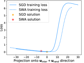
Refer to caption
Refer to caption
Refer to caption
Figure 29: The average of SGD has a bias on flat side (ResNet-164 on CIFAR-100).

Examples for asymmetric directions of ResNet-110 on CIFAR-10 in Figure 30.
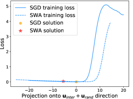
Refer to caption
Refer to caption
Refer to caption
Figure 30: The average of SGD has a bias on flat side (ResNet-110 on CIFAR-10).

Appendix H Additional Figure for Section 6.3: Width of Minima
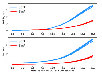
See Figure 31, similar results were observed by (Izmailov et al., 2018) as well.

Refer to caption
Figure 31: Random ray of SGD and SWA solution

Appendix I Additional Figures for Section 7: BN Parameters Are More Asymmetric
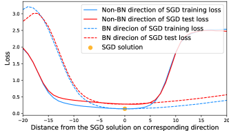
See Figure 32, Figure 33 and Figure 34.

Refer to caption
Figure 32: BN and Non-BN directions comparison of ResNet-164 on CIFAR-10
Refer to caption
Figure 33: BN and Non-BN directions comparison of ResNet-110 on CIFAR-100
Refer to caption
Figure 34: BN and Non-BN directions comparison of DenseNet-100 on CIFAR-100