Self-Binarizing Networks

Abstract

We present a method to train self-binarizing neural networks, that is, networks that evolve their weights and activations during training to become binary. To obtain similar binary networks, existing methods rely on the sign activation function. This function, however, has no gradients for non-zero values, which makes standard backpropagation impossible. To circumvent the difficulty of training a network relying on the sign activation function, these methods alternate between floating-point and binary representations of the network during training, which is sub-optimal and inefficient. We approach the binarization task by training on a unique representation involving a smooth activation function, which is iteratively sharpened during training until it becomes a binary representation equivalent to the sign activation function. Additionally, we introduce a new technique to perform binary batch normalization that simplifies the conventional batch normalization by transforming it into a simple comparison operation. This is unlike existing methods, which are forced to the retain the conventional floating-point-based batch normalization. Our binary networks, apart from displaying advantages of lower memory and computation as compared to conventional floating-point and binary networks, also show higher classification accuracy than existing state-of-the-art methods on multiple benchmark datasets.

1 Introduction

Deep learning has brought about remarkable advancements to the state-of-the-art in several fields including computer vision and natural language processing. In particular, convolutional neural networks (CNN’s) have shown state-of-the-art performance in several tasks such as object recognition with AlexNet (Krizhevsky et al., 2012), VGG (Simonyan & Zisserman, 2014), ResNet (He et al., 2016) and detection with R-CNN (Girshick et al., 2014; Girshick, 2015; Ren et al., 2017). However, to achieve real-time performance these networks are dependent on specialized hardware like GPU’s because they are computation and memory demanding. For example, AlexNet takes up 250Mb for its 60M parameters while VGG requires 528Mb for its 138M parameters.

While the performance of deep networks has been gradually improving over the last few years, their computational speed has been steadily decreasing (Vedaldi, 2016). Notwithstanding this, interest has grown significantly in the deployment of CNN’s in virtual reality headsets (Oculus, GearVR), augmented reality gear (HoloLens, Epson Moverio), and other wearable, mobile, and embedded devices. While such devices typically have very restricted power and memory capacites, they demand low latency and real-time performance to be able to provide a good user experience. Not surprisingly, there is considerable interest in making deep learning models computationally efficient to better suit such devices (Ota et al., 2017; Cheng et al., 2018; Zhu, 2018).

Several methods of compression, quantization, and dimensionality reduction have been introduced to lower memory and computation requirements. These methods produce near state-of-the-art results, either with fewer parameters or with lower precision parameters, which is possible thanks to the redundancies in deep networks (Cheng et al., 2015).

In this paper we focus on the solution involving binarization of weights and activations, which is the most extreme form of quantization. Binarized neural networks achieve high memory and computational efficiency while keeping performance comparable to their floating point counterparts.  Courbariaux et al. (2015) have shown that binary networks allow the replacement of multiplication and additions by simple bit-wise operations, which are both time and power efficient.

The challenge in training a binary neural network is to convert all its parameters from the continuous domain to a binary representation, typically done using the $\operatorname{sign}$ activation function. However, since the gradient of $\operatorname{sign}$ is zero for all nonzero inputs, it makes standard back-propagation impossible. Existing state-of-the-art methods for network binarization (Courbariaux et al., 2015; 2016; Rastegari et al., 2016) alternate between a binarized forward pass and a floating point backward pass to circumvent this problem. In their case, the gradients for the $\operatorname{sign}$ activation are approximated during the backward pass, thus introducing inaccuracies in training. Furthermore, batch normalization (Ioffe & Szegedy, 2015) is necessary in binary networks to avoid exploding feature map values due to the large scale of the weights. However, during inference, using batch normalization introduces intermediary floating point representations. This means, despite binarizing weights and activations, these networks can not be used on chips that do not support floating-point computations.

In our method, the scaled hyperbolic tangent function $\tanh$ is used to bound the values in the range $[-1,1]$. The network starts with floating point values for weights and activations, and progressively evolves into a binary network as the scaling factor is increased. Firstly, this means that we do not have to toggle between the binary and floating point weight representations. Secondly, we have a continuously differentiable function that allows backpropagation passes. As another important contribution, we reduce the standard batch normalization operation during the inference stage to a simple comparison. This modification is not only very efficient and can be accomplished using fixed-point operations, it is also an order of magnitude faster than the floating-point counterpart. More clearly, while existing binarization methods perform, at each layer, the steps of binary convolutions, floating-point batch normalization, and sign activation, we only need to perform binary convolutions followed by our comparison-based batch normalization, which serves as the sign activation at the same time.

We validate the performance of our self-binarizing networks by comparing them to those of existing binarization methods. We choose the standard bechmarks of CIFAR-10, CIFAR-100 (Krizhevsky & Hinton, 2009) as well as ImageNet (Russakovsky et al., 2015) and popular network architectures such as VGG and AlexNet. We demonstrate higher accuracies despite using less memory and fewer computations. To the best of our knowledge, our proposed networks are the only ones that are free of any floating point computations and can therefore be deployed on low-precision integrated chips or micro-controllers.

In what follows, in Sec. 2 we describe previous work related to reducing the network complexity and where we are placed among them. In Sec. 3 we explain how the scaled $\tanh$ function can be used for progressive binarization. In Sec. 4 we explain our binarization method for weights and activations and explain how to simplify batch normalization at inference time. In Sec. 5 we compare our technique to existing state-of-the-art binary networks on standard benchmarks and demonstrate the performance gains from our proposed batch normalization simplification. Sec. 6 concludes the paper.

2 Related Work

Making deep networks memory and computation efficient has been approached in various ways. In this section we cover some of the relevant literature and explain how our work is positioned with respect to the state-of-the-art. The interested reader may refer to Cheng et al. (2018), Ota et al. (2017), and Zhu (2018) for a wider coverage.

Since most of the computation in deep networks is due to convolutions, it is logical to focus on reducing the computational burden due to them. Howard et al. (2017); Zhang et al. (2017); Freeman et al. (2018) employ variations of convolutional layers by taking advantage of the separability of the kernels either by convolving with a group of input channels or by splitting the kernels across the dimensions. In addition to depth-wise convolutions, MobileNetV2 (Sandler et al., 2018) uses inverted residual structures to learn how to combine the inputs in a residual block. In general, these methods try to design a model that computes convolutions in an efficient manner. This is different from this work because it focuses on redesigning the structure of the network, while ours tries to reduce the memory requirements by using lower precision parameters. However, our method can be applied to these networks as well.

Reducing the number of weights likewise reduces the computational and memory burden. Due to the redundancy in deep neural networks (Cheng et al., 2015), there are some weights that contribute more to the output than others. The process of removing the less contributing weights is called pruning. In LeCun et al. (1990), the contribution of weights is measured by the effect on the training error when this parameter is zeroed. In Deep Compression (Han et al., 2015), the weights with lowest absolute value are pruned and the remaining are quantized and compressed using Huffman coding. In other work, Fisher Information (Tu et al., 2016) is used to measure the amount of information the output carries about each parameter, which allows pruning. While these approaches often operate on already trained networks and fine-tune them after compression, our method trains a network to a binary state from scratch without removing any parameters or feature maps. This allows us to retain the original structure of the network, while still leaving the potential for further compression after or during binarization using pruning techniques.

Another way to reduce memory consumption and potentially improve computational efficiency is the quantization of weights. Quantized neural networks (Hubara et al., 2016; Zhou et al., 2016; 2017) occupy less memory while retaining similar performance as their full precision counterparts. DoReFaNet (Zhou et al., 2016) proposes to train low bitwidth networks with low bitwidth gradients using stochastic quantization. Similarly, Zhou et al. (2017) devise a weight partitioning technique to incrementally quantize the network at each step. The degree of quantization can vary between techniques.  Deng et al. (2018), Zhu et al. (2016), and Li & Liu (2016) quantize weights to three levels, i.e., two bits only. These quantizations, while severe, still allow for accurate inference. However, to improve computational efficency, specialized hardware is needed to take advantage of the underlying ternary operations.

An extreme form of such quantization is binarization, which requires only one bit to represent. Expectation BackPropagation (EBP) paved the way for training neural networks for precision limited-hardware (Soudry et al., 2014). BinaryConnect (Courbariaux et al., 2015) extended the idea to train neural networks with binary weights. The authors later propose BinaryNet (Courbariaux et al., 2016) to binarize activations as well. Similarly, XNORNet (Rastegari et al., 2016) extends BinaryNet by adding a scaling factor to the parameters of every layer while keeping the weights and activations binary. ABCNet (Lin et al., 2017) approximates full precision parameters as a linear combination of binary weights and uses multiple binary activations to compensate for the information loss arising from quantization. Hou et al. (2016) use Hessian approximations to minimize loss with respect to the binary weights during training.

The focus of our work is the binarization of weights and activations of a network. In previous binarization methods, the binarization process is non-differentiable leading to approximations during the training that can affect the final accuracy. In contrast, we use a differentiable function to progressively self-binarize the network and improve its accuracy. Additionally, we differ from these techniques as we introduce a comparison-based binary batch normalization that eliminates all floating point operations at inference time.

3 Self-binarization with Tanh

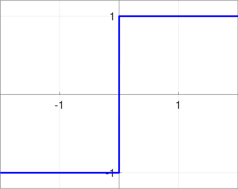
In typical binary network training, during the forward pass, the floating-point weights and activations are quantized to binary values $\{-1,1\}$, through a piece-wise constant function, most commonly the $\operatorname{sign}$ function:

$$\operatorname{sign}(x)=\begin{cases}-1&\textrm{if }x\leq 0\\ 1&\textrm{if }x>0.\end{cases}$$ (1)

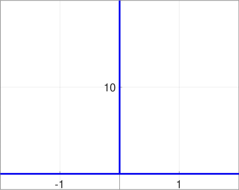
This non-linear activation leads to strong artifacts during the forward pass, and does not generate gradients for backpropagation. The derivatives of the binarized weights are therefore approximately computed using a Straight Through Estimator (STE) (Bengio et al., 2013). STE creates non-zero derivative approximations for functions that either have a zero derivative everywhere or are non-differentiable. Typically, the derivative of $\operatorname{sign}$ is estimated by using the following STE:

$$\frac{\partial\operatorname{sign}(x)}{\partial x}=\begin{cases}1&\textrm{if }|x|\leq 1\\ 0&\textrm{otherwise}.\end{cases}$$ (2)

In the backward propagation step, the gradients are computed on the binarized weights using the STE and the corresponding floating-point representations are updated. Since both forward and backward functions are different, the training is ill-defined. The lack of an accurate derivative for the weights and activations creates a mismatch between the quantized and floating-point values and influences learning accuracy. We term this as hard binarization.

This kind of problems has been studied previously, and continuation methods have been proposed to simplify its solution (Allgower & Georg, 2003). To do so, the original complex and non-smooth optimization problem is transformed by smoothing the original function and then gradually decreasing the smoothness during training, building a sequence of sub-optimization problems converging to the original one. For example, Cao et al. (2017) apply these methods on the last layer of a neural network to predict hashes from images.

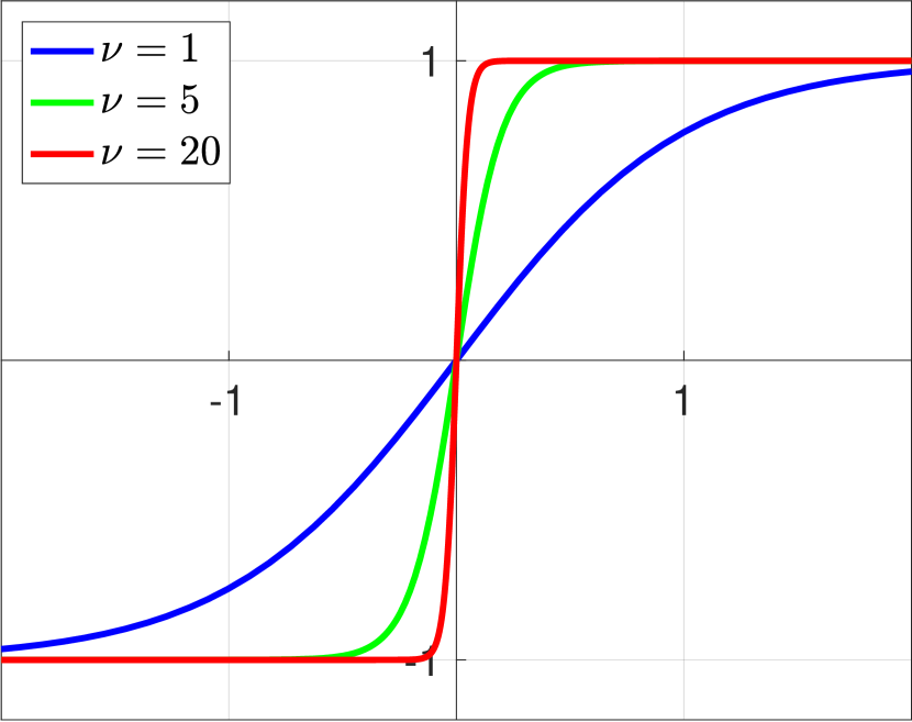
Following this philosophy, we introduce a much simpler and efficient training method that allows the network to self-binarize. We pass all our weights and activations through the hyperbolic tangent function $\tanh$ whose slope can be varied using a scale parameter $\nu>0$. As seen in Fig. 1(c), when $\nu$ is large enough the $\tanh(\nu x)$ converges to the $\text{sign}(x)$ function:

$$\lim_{\nu\rightarrow\infty}{\tanh(\nu x)}=\operatorname{sign}(x).$$ (3)

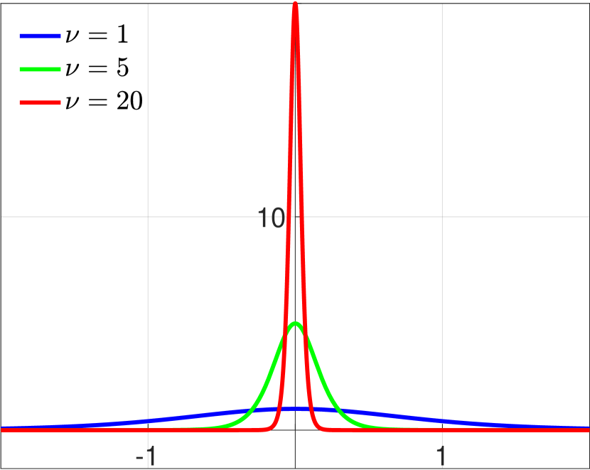
Throughout the training process, the weights and activations use floating-point values. Starting from a value of $\nu=1$, as the scale factor is progressively incremented, the weights and activations are forced to attain binary values $\{-1,1\}$. During the training and while $\nu$ is still small, the derivative of $\tanh$ exists for every value of $x$ and is expressed as

$$\frac{\partial\tanh(\nu x)}{\partial x}=\nu\operatorname{sech}^{2}(\nu x)=\nu(1-\tanh^{2}(\nu x)),$$ (4)

where $\operatorname{sech}$ is the hyperbolic secant. Using the scaled $\tanh$, we can build a continuously differentiable network which progressively approaches a binary state, leading to a more principled approach to obtain a binarized network. We term this approach as soft binarization.

(a) $\operatorname{sign}(x)$

(b) $\delta(x)$

(c) $\tanh(\nu x)$

(d) $\nu\text{sech}^{2}(\nu x)$

Figure 1: The discrete $\operatorname{sign}$ (a) and its derivative (b) are shown. (c, d) show that as $\nu$ takes values of 1, 5, and 20, the scaled $\tanh$ converges toward the original $\operatorname{sign}$ function and its derivative.

4 Method

In this section, we formally describe our self-binarizing approach. We first explain how weights and activations are binarized. Then, we propose a more efficient, comparison-based batch-normalization method that is more suitable when working in binary settings.

4.1 Weight self-binarization

As stated above, we cannot use binary weights at training time as it would make gradient computation infeasible. Instead, we use a set of constrained floating-point weights $\mathbf{W}_{\ell}$ at each layer $\ell$. Unlike traditional networks, these weights are not learnable parameters of our model, but depend on learnable parameters. For each layer $\ell$ of the network, we define a set of learnable, unconstrained parameters $\mathbf{P}_{\ell}$ and use the scaled $\tanh$ to compute the weights as

$$\mathbf{W}_{\ell}=\tanh(\nu_{e}\mathbf{P}_{\ell}),$$ (5)

where $\nu_{e}$ is the scale factor at epoch $e$, taken from a sequence $1=\nu_{0}<\nu_{1}<\ldots<\nu_{M}\rightarrow\infty$ of increasingly larger values. During training, parameters $\mathbf{P}_{\ell}$ are updated to minimize a loss function using a standard gradient-based optimization procedure, such as stochastic gradient descent. The scaled $\tanh$ transforms the parameters $\mathbf{P}_{\ell}$ to obtain weights $\mathbf{W}_{\ell}$ that are bounded in the range $[-1,1]$ and become closer to binary values as the training proceeds.

At the end of the training, weights $\mathbf{W}_{\ell}$ are very close to exact binary values. At this point, we obtain the final binary weights $\mathbf{B}_{\ell}$ by taking the sign of the parameters,

$$\mathbf{B}_{\ell}=\operatorname{sign}(\mathbf{P}_{\ell})\approx\mathbf{W}_{\ell},\quad\forall r.$$ (6)

At inference time, we drop all learnable parameters $\mathbf{P}_{\ell}$ and constrained weights $\mathbf{W}_{\ell}$, and use only binary weights $\mathbf{B}_{\ell}$.

4.2 Activation self-binarization

We follow the idea as for weights to address the binarization of activations as well. During training, we use the scaled $\tanh$ as the activation function of the network. For a given layer $\ell$, the activation function transforms the output $\mathbf{O}_{\ell}$ of the layer to lead to the activation

$$\mathbf{A}_{\ell}=\tanh(\nu_{e}\mathbf{O}_{\ell}).$$ (7)

The activations are constrained to lie within the range $[-1,1]$, and eventually become binary at the end of the training procedure. At inference time we make the network completely binary by substituting the scaled $\tanh$ by the $\operatorname{sign}$ operator as the binary activation function.

4.3 Binary Batch Normalization (BinaryBN)

Batch Normalization (BN) introduced by Ioffe & Szegedy (2015) accelerates the training of a general deep network. During training, the BN layers compute the running mean $\mu_{r}$ and standard deviation $\sigma_{r}$ of the feature maps that pass through them, as well as two parameters, $\beta$ and $\gamma$, that define an affine transformation. Later, at inference time, BN layers normalize and transform the input $I$ to obtain an output $O$ as given by

$$O=\dfrac{I-\mu_{r}}{\sigma_{r}}\gamma+\beta.$$ (8)

For binary networks (Courbariaux et al., 2015; 2016; Rastegari et al., 2016) in particular, BN becomes essential in order to avoid exploding activation values. However, using BN brings in the limitation of relying on floating-point computations. Apart from affecting computation and memory requirements, the floating-point BN effectively eliminates the possibility of using the network on low-precision hardware.

A useful observation of BN is that, in a networks with binary activations, the output of the BN layers is always fed into a $\operatorname{sign}$ function. This means only the sign of the normalized output is kept, while its magnitude is not relevant for the subsequent layers. We can leverage this property to simplify the BN operation. The sign of the output $O$ of a BN layer can be reformulated as:

$$\begin{split}\operatorname{sign}(O)&\equiv O>0\equiv\frac{I-\mu_{r}}{\sigma_{r}}\gamma+\beta>0\\ &\equiv(I-\mu_{r})\gamma>-\sigma_{r}\beta\\ &\equiv I\operatorname{sign}(\gamma)>\left(\mu_{r}-\frac{\sigma_{r}\beta}{\gamma}\right)\operatorname{sign}(\gamma)\quad\text{since dividing by}\ \gamma\ \text{could flip the inequality}\\ &\equiv I\operatorname{sign}(\gamma)>T\operatorname{sign}(\gamma)\\ &\equiv\text{XNOR}(I>T,\gamma>0),\end{split}$$ (9)

with

$$T=\mu_{r}-\frac{\sigma_{r}\beta}{\gamma}.$$ (10)

While $T$ is a floating-point value, in practice we represent it as a fixed-point 8-bit integer. This sacrifices some amount of numerical precision, but we observed no negative effect on the performance of our models. We refer to our simplified batch normalization as Binary Batch Normalization (BinaryBN).

Note that the derivation of Eq. (9) does not hold when $\gamma=0$. This is handled as a special case that simply evaluates $\beta>0$. It must be emphasized that BinaryBN is not an approximate method; it computes the exact value of the sign of the output of the standard BN.

During training we use the conventional BN layers. At inference time, we replace them with the BinaryBN without any loss in prediction accuracy. Our trained models can thus bypass the floating-point batch normalization with an efficient alternative that requires mere comparison operations.

5 Experiments

In this section, we first compare our self-binarization method against other known techniques. Later on, we discuss and demonstrate the efficiency gained using our proposed BinaryBN instead of the typical BN layer.

5.1 Classification Accuracy

We compare our self-binarizing networks with other state-of-the-art methods that use binary networks.  Courbariaux et al. (2015) present BinaryConnect (BC), a method that only binarizes the weights. Binary Neural Networks (BNN) (Courbariaux et al., 2016) improves BC by also binarizing the activations. Similarly, Rastegari et al. (2016) present two variants of their method: Binary Weight Networks (BWN), which only binarizes the weights, and XNORnet (XNOR), which binarizes both weights and activations.

For a fair comparison and to prove the generality of our method, we use the original implementations of BC, BNN, BWN, and XNOR, and apply our self-binarizing technique to them. Specifically, we substituted the weights from the original implementations by a pair of parameters $\mathbf{P}$ and constrained weights $\mathbf{W}$ given by Eq. (5). Also, we substituted the activation functions by the scaled $\tanh$ as described in Eq. (7). At inference time we used the binary weights obtained with Eq. (6) and the $\operatorname{sign}$ operator as the activation function. Additionally, we replace the batch normalization layers by our BinaryBN layer for the cases where the activations are binarized.

We evaluate the methods on three common benchmark datasets: CIFAR-10, CIFAR-100 (Krizhevsky & Hinton, 2009) and ILSVRC12 ImageNet (Russakovsky et al., 2015). For CIFAR-10 and CIFAR-100, we use a VGG-16-like network with data augmentation as proposed in Lee et al. (2015): 4 pixels are padded on each side, and a 32x32 patch is randomly cropped from the padded image or its horizontal flip. During testing, only a single view of the original 32x32 image is evaluated. The model is trained with a mini-batch size of 256 for 100 epochs.

The ILSVRC12 ImageNet dataset is used to train an AlexNet-like network without drop-out or local response normalization layers. We use the data augmentation strategy from Wu et al. (2016). At inference time, only the center crop is used from the validation set. The model is trained with a mini-batch size of 64 and a total of 50 epochs.

In all our experiments we increase $\nu$ from $1$ to $1000$ during training in an exponential manner. The final $\nu=1000$ is large enough to make weights and activations almost binary in practice. We optimize all models using Adam (Kingma & Ba, 2014) with an exponentially decaying learning rate starting at $10^{-3}$.

Table 1: Accuracy rates (%) comparing existing state-of-the-art methods when trained with and without our self-binarizing technique. Top-1 and Top-5 results are reported for CIFAR-100 and ImageNet. Also, Top-1 results are reported for CIFAR-10. $B_{w}$, $B_{a}$, and $B_{BN}$ indicate the number of bits required to represent the values of the weights, activations, and batch normalization outputs. Note that since we use BinaryBN, which combines the batch normalization and activation steps, we do not show any bits for $B_{a}$ when both weights and activations are binarized using our method.

	Method		$B_{w}$	$B_{a}$	$B_{BN}$	CIFAR-10	CIFAR-100	ImageNet
	Full-Precision		32	32	32	86.55	60.67 / 81.98	55.07 / 79.27
WEIGHT-ONLY BINARIZATION	BC	orig.	1	32	32	87.24	55.82 / 73.11	40.57 / 66.40
		ours	1	32	32	88.50	55.81 / 76.50	41.27 / 67.51
	BWN	orig.	1	32	32	89.87	63.14 / 85.64	50.87 / 75.63
		ours	1	32	32	90.56	63.48 / 86.01	52.89 / 77.34
WEIGHT & ACTIVATION BINARIZATION	BNN	orig.	1	1	32	84.06	51.58 / 78.58	29.94 / 56.43
		ours	1	-	1	84.61	54.06 / 80.45	30.97 / 56.65
	XNOR	orig.	1	1	32	86.16	51.91 / 79.41	37.84 / 64.06
		ours	1	-	1	86.91	53.84 / 81.56	39.44 / 65.23

Table 1 shows the results of the experiments. Our self-binarizing approach achieves the highest accuracies for CIFAR-10 and ImageNet. Our method is only slightly outperformed by BC for CIFAR-100, but still gives better Top-5 accuracy for the same model. For both weights and activation binarization, our method obtains the best results across all datasets and architectures.

What is remarkable is that the improved performance comes despite eliminating floating-point computations and using drastically fewer bits than the previous methods, as can be seen in the columns $B_{w}$, $B_{a}$ and $B_{BN}$ of Table 1. For CIFAR-10 and CIFAR-100, BWN outperforms the full precision models likely because the binarization serves as a regularizer (Courbariaux et al., 2015).

5.2 Efficiency due to BinaryBN

With all other computations being common between our self-binarizing networks and other networks with binary weights and activations, any difference in computational efficiency has to arise from the use of a different batch normalization scheme. We therefore compare our proposed BinaryBN layer to the conventional BN layer as well as to the Shift-based Batch Normalization (SBN) proposed by Courbariaux et al. (2016). SBN proposes to round both $\gamma$ and $\sigma_{r}$ to their nearest power of 2 and replace multiplications and divisions by left and right shifts, respectively. SBN follows the same formula as BN, and is used both at training and inference time, so that the network is trained with the rounded parameters.

Table 2: Memory and computational requirements of BN, SBN and BinaryBN layers when working on a $w\times h$ feature map with $c$ channels.

	BN + $\operatorname{sign}$	SBN + $\operatorname{sign}$	BinaryBN
Operations used	$+,-,\times,\div$	$+,-,\ll,\gg$	$>,=$
Storage Memory	$128c$	$80c$	$9c$
Output Memory	$32chw+chw$	$32chw+chw$	$chw$
Operations	$4chw+chw$	$4chw+chw$	$2chw$

Table. 2 summarizes the requirements of memory and computational time of these three types of batch normalization layers. We assume the standard case where a binary convolution is followed by a batch normalization layer and then a binary activation function.

For storing BN parameters, we need four 32-bit vectors of length $c$, amounting to $32\times 4c=128c$ bits, $c$ being the number of channels in this layer. For SBN, we need two 32-bit vectors and two 8-bit vectors of length $c$, resulting in $80c$ bits. For BinaryBN, we need an 8-bit vector of size $c$ to store the $T$ value of each channel, and a binary vector for the sign of $\gamma$, totaling $9c$ bits.

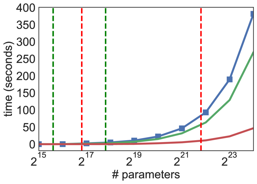
(a) Time comparison

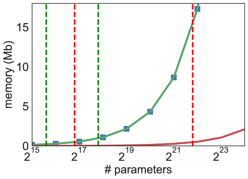
(b) Memory comparison

Figure 2: Comparison between time and memory consumption of BN, SBN and BinaryBN for an input feature map of $256\times 256$. For reference, dotted lines show the minimum and maximum number of parameters that can be found in the BN layers of a VGG-16 network and an AlexNet network.

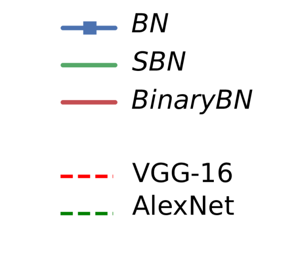
We experimentally assessed the time and memory requirements of the three batch normalization techniques. We run batches of increasing sizes through BN, SBN and BinaryBN layers with randomly generated values for $\mu_{r}$, $\sigma_{r}$, $\beta$, and $\gamma$, and measure time and memory consumption. Fig. 2 shows the results. Overall, BinaryBN is nearly one order of magnitude less memory consuming and faster than BN and SBN.

5.3 Why soft binarization is better

In order to show the superiority of our soft binarization based on scaled $\tanh$ over the hard binarization of BC, BNN, BWN, and XNOR, we take snapshots of the weights at different epochs of training a VGG-16 network on CIFAR10. Fig. 3 shows the histograms of snapshots taken at the last convolutional layer of the network. It can be seen that, under the soft binarization scheme, the floating-point weights are initially centered at $0$, allowing them to continue evolving as the network progresses. As the training proceeds, the distribution of softly-binarized weights is gradually shifted towards binary values. However, under the hard binarization scheme, the distribution of floating-point weights is not similarly centered at zero, which means a lot of the weights have immediately been driven far from $0$ and require very large gradients to be changed. With weights unable to change as much, a lot of the neurons in the network become quickly unusable thereby limiting the final performance of the architecture. This explains why our binary networks perform better than those relying on hard binarization.

(a) Hard binarization with $\text{sign}(x)$

(b) Soft binarization with $\tanh(\nu x)$

Figure 3: Histograms of weights before (blue) and after (red) binarization for conventional approaches in (a) versus our method in (b).

6 Conclusion

We present a novel method to binarize a deep network that is principled, simple, and results in binarization of weights and activations. Instead of relying on the $\operatorname{sign}$ function, we use the $\tanh$ function with a controllable slope. This simplifies the training process without breaking the flow of derivatives in the back-propagation phase as compared to that of existing methods that have to toggle between floating-point and binary representations. In addition to this, we replace the conventional batch normalization, which forces existing binarization methods to use floating point computations, by a simpler comparison operation that is directly adapted to networks with binary activations. Our simplified batch normalization is not only computationally trivial, it is also extremely memory-efficient. Despite using lesser memory and computation, our trained binary networks outperform those of existing binarization schemes on the standard benchmarks.

References

- Allgower & Georg (2003) Eugene L Allgower and Kurt Georg. Introduction to numerical continuation methods, volume 45. SIAM, 2003.
- Bengio et al. (2013) Yoshua Bengio, Nicholas Léonard, and Aaron Courville. Estimating or propagating gradients through stochastic neurons for conditional computation. arXiv preprint arXiv:1308.3432, 2013.
- Cao et al. (2017) Zhangjie Cao, Mingsheng Long, Jianmin Wang, and Philip S Yu. Hashnet: Deep learning to hash by continuation. arXiv preprint arXiv:1702.00758, 2017.
- Cheng et al. (2015) Yu Cheng, Felix X Yu, Rogerio S Feris, Sanjiv Kumar, Alok Choudhary, and Shi-Fu Chang. An exploration of parameter redundancy in deep networks with circulant projections. In Proceedings of the IEEE International Conference on Computer Vision, pp. 2857–2865, 2015.
- Cheng et al. (2018) Yu Cheng, Duo Wang, Pan Zhou, and Tao Zhang. Model compression and acceleration for deep neural networks: The principles, progress, and challenges. IEEE Signal Processing Magazine, 35(1), January 2018.
- Courbariaux et al. (2015) Matthieu Courbariaux, Yoshua Bengio, and Jean-Pierre David. Binaryconnect: Training deep neural networks with binary weights during propagations. In Advances in neural information processing systems, pp. 3123–3131, 2015.
- Courbariaux et al. (2016) Matthieu Courbariaux, Itay Hubara, Daniel Soudry, Ran El-Yaniv, and Yoshua Bengio. Binarized neural networks: Training deep neural networks with weights and activations constrained to+ 1 or-1. arXiv preprint arXiv:1602.02830, 2016.
- Deng et al. (2018) Lei Deng, Peng Jiao, Jing Pei, Zhenzhi Wu, and Guoqi Li. Gxnor-net: Training deep neural networks with ternary weights and activations without full-precision memory under a unified discretization framework. Neural Networks, 100:49–58, 2018.
- Freeman et al. (2018) Ido Freeman, Lutz Roese-Koerner, and Anton Kummert. Effnet: An efficient structure for convolutional neural networks. arXiv preprint arXiv:1801.06434, 2018.
- Girshick (2015) Ross Girshick. Fast r-cnn. arXiv preprint arXiv:1504.08083, 2015.
- Girshick et al. (2014) Ross Girshick, Jeff Donahue, Trevor Darrell, and Jitendra Malik. Rich feature hierarchies for accurate object detection and semantic segmentation. In Proceedings of the IEEE conference on computer vision and pattern recognition, pp. 580–587, 2014.
- Han et al. (2015) Song Han, Huizi Mao, and William J Dally. Deep compression: Compressing deep neural networks with pruning, trained quantization and huffman coding. arXiv preprint arXiv:1510.00149, 2015.
- He et al. (2016) Kaiming He, Xiangyu Zhang, Shaoqing Ren, and Jian Sun. Deep residual learning for image recognition. In Proceedings of the IEEE conference on computer vision and pattern recognition, pp. 770–778, 2016.
- Hou et al. (2016) Lu Hou, Quanming Yao, and James T Kwok. Loss-aware binarization of deep networks. arXiv preprint arXiv:1611.01600, 2016.
- Howard et al. (2017) Andrew G Howard, Menglong Zhu, Bo Chen, Dmitry Kalenichenko, Weijun Wang, Tobias Weyand, Marco Andreetto, and Hartwig Adam. Mobilenets: Efficient convolutional neural networks for mobile vision applications. arXiv preprint arXiv:1704.04861, 2017.
- Hubara et al. (2016) Itay Hubara, Matthieu Courbariaux, Daniel Soudry, Ran El-Yaniv, and Yoshua Bengio. Quantized neural networks: Training neural networks with low precision weights and activations. arXiv preprint arXiv:1609.07061, 2016.
- Ioffe & Szegedy (2015) Sergey Ioffe and Christian Szegedy. Batch normalization: Accelerating deep network training by reducing internal covariate shift. arXiv preprint arXiv:1502.03167, 2015.
- Kingma & Ba (2014) Diederik Kingma and Jimmy Ba. Adam: A method for stochastic optimization. 12 2014.
- Krizhevsky & Hinton (2009) Alex Krizhevsky and Geoffrey Hinton. Learning multiple layers of features from tiny images. 2009.
- Krizhevsky et al. (2012) Alex Krizhevsky, Ilya Sutskever, and Geoffrey E Hinton. Imagenet classification with deep convolutional neural networks. In Advances in neural information processing systems, pp. 1097–1105, 2012.
- LeCun et al. (1990) Yann LeCun, John S Denker, and Sara A Solla. Optimal brain damage. In Advances in neural information processing systems, pp. 598–605, 1990.
- Lee et al. (2015) Chen-Yu Lee, Saining Xie, Patrick Gallagher, Zhengyou Zhang, and Zhuowen Tu. Deeply-supervised nets. In Artificial Intelligence and Statistics, pp. 562–570, 2015.
- Li & Liu (2016) Fengfu Li and Bin Liu. Ternary weight networks. CoRR, abs/1605.04711, 2016. URL http://arxiv.org/abs/1605.04711.
- Lin et al. (2017) Xiaofan Lin, Cong Zhao, and Wei Pan. Towards accurate binary convolutional neural network. In Advances in Neural Information Processing Systems, pp. 344–352, 2017.
- Ota et al. (2017) Kaoru Ota, Minh Son Dao, Vasileios Mezaris, and Francesco G. B. De Natale. Deep learning for mobile multimedia: A survey. ACM Trans. Multimedia Comput. Commun. Appl., 13(3s):34:1–34:22, June 2017. ISSN 1551-6857. doi: 10.1145/3092831. URL http://doi.acm.org/10.1145/3092831.
- Rastegari et al. (2016) Mohammad Rastegari, Vicente Ordonez, Joseph Redmon, and Ali Farhadi. Xnor-net: Imagenet classification using binary convolutional neural networks. In European Conference on Computer Vision, pp. 525–542. Springer, 2016.
- Ren et al. (2017) Shaoqing Ren, Kaiming He, Ross Girshick, and Jian Sun. Faster r-cnn: towards real-time object detection with region proposal networks. IEEE transactions on pattern analysis and machine intelligence, 39(6):1137–1149, 2017.
- Russakovsky et al. (2015) Olga Russakovsky, Jia Deng, Hao Su, Jonathan Krause, Sanjeev Satheesh, Sean Ma, Zhiheng Huang, Andrej Karpathy, Aditya Khosla, Michael Bernstein, et al. Imagenet large scale visual recognition challenge. International Journal of Computer Vision, 115(3):211–252, 2015.
- Sandler et al. (2018) Mark Sandler, Andrew Howard, Menglong Zhu, Andrey Zhmoginov, and Liang-Chieh Chen. Inverted residuals and linear bottlenecks: Mobile networks for classification, detection and segmentation. arXiv preprint arXiv:1801.04381, 2018.
- Simonyan & Zisserman (2014) Karen Simonyan and Andrew Zisserman. Very deep convolutional networks for large-scale image recognition. arXiv preprint arXiv:1409.1556, 2014.
- Soudry et al. (2014) Daniel Soudry, Itay Hubara, and Ron Meir. Expectation backpropagation: Parameter-free training of multilayer neural networks with continuous or discrete weights. In Advances in Neural Information Processing Systems, pp. 963–971, 2014.
- Tu et al. (2016) Ming Tu, Visar Berisha, Martin Woolf, Jae-sun Seo, and Yu Cao. Ranking the parameters of deep neural networks using the fisher information. In Acoustics, Speech and Signal Processing (ICASSP), 2016 IEEE International Conference on, pp. 2647–2651. IEEE, 2016.
- Vedaldi (2016) Andrea Vedaldi. Convolutional networks for computer vision applications, February 2016. URL http://www.robots.ox.ac.uk/~vedaldi/assets/teach/vedaldi16deepcv.pdf.
- Wu et al. (2016) Yuxin Wu et al. Tensorpack. https://github.com/tensorpack/, 2016.
- Zhang et al. (2017) Xiangyu Zhang, Xinyu Zhou, Mengxiao Lin, and Jian Sun. Shufflenet: An extremely efficient convolutional neural network for mobile devices. arXiv preprint arXiv:1707.01083, 2017.
- Zhou et al. (2017) Aojun Zhou, Anbang Yao, Yiwen Guo, Lin Xu, and Yurong Chen. Incremental network quantization: Towards lossless cnns with low-precision weights. arXiv preprint arXiv:1702.03044, 2017.
- Zhou et al. (2016) Shuchang Zhou, Yuxin Wu, Zekun Ni, Xinyu Zhou, He Wen, and Yuheng Zou. Dorefa-net: Training low bitwidth convolutional neural networks with low bitwidth gradients. arXiv preprint arXiv:1606.06160, 2016.
- Zhu et al. (2016) Chenzhuo Zhu, Song Han, Huizi Mao, and William J Dally. Trained ternary quantization. arXiv preprint arXiv:1612.01064, 2016.
- Zhu (2018) Ji Wang ; Bokai Cao ; Philip Yu ; Lichao Sun ; Weidong Bao ; Xiaomin Zhu. Deep learning towards mobile applications. In International Conference on Distributed Computing Systems (ICDCS), 2018.