Identifying Variability in Deeply Embedded Protostars with ALMA and CARMA

Abstract

Variability of pre-main-sequence stars observed at optical wavelengths has been attributed to fluctuations in the mass accretion rate from the circumstellar disk onto the forming star. Detailed models of accretion disks suggest that young deeply embedded protostars should also exhibit variations in their accretion rates, and that these changes can be tracked indirectly by monitoring the response of the dust envelope at mid-IR to millimeter wavelengths. Interferometers such as ALMA offer the resolution and sensitivity to observe small fluctuations in brightness at the scale of the disk where episodic accretion may be driven. In this work, we present novel methods for comparing interferometric observations and apply them to CARMA and ALMA 1.3mm observations of deeply embedded protostars in Serpens taken 9 years apart. We find no brightness variation above the limits of our analysis of a factor of $\gtrsim 50\%$, due to the limited sensitivity of the CARMA observations and small number of sources common to both epochs. We further show that follow up ALMA observations with a similar sample size and sensitivity may be able to uncover variability at the level of a few percent, and discuss implications for future work.

1. Introduction

The earliest stages of star formation begin with the gravitational collapse of a molecular cloud core to a protostar and circumstellar disk, both surrounded by an extended envelope of gas and dust. The disk is fed by infall of mass from the envelope, while further growth of the protostar proceeds by accretion from the disk. The transport of mass through the disk and onto the protostar is predicted to produce a varying accretion rate by a wide variety of mechanisms, including gravitational and/or magneto-rotational instabilities in the disk (e.g., Armitage et al. 2001; Vorobyov & Basu 2005, 2006, 2010; Machida et al. 2011; Cha & Nayakshin 2011; Zhu et al. 2009a, b, 2010; Bae et al. 2014; Hartmann et al. 2016), quasi-periodic magnetically driven outflows in the envelope (Tassis & Mouschovias, 2005), decay and regrowth of magneto-rotational instability turbulence (Simon et al., 2011), close interaction in binary systems or in dense stellar clusters (Bonnell & Bastien 1992; Pfalzner et al. 2008), and disk/planet interactions (Lodato & Clarke 2004; Nayakshin & Lodato 2012).

A variable accretion rate can also resolve the “luminosity problem” (Kenyon et al., 1990; Dunham et al., 2010, 2014), the discrepancy between the observed luminosities of protostars, which are spread over several orders of magnitude (Dunham et al., 2015; Jensen & Haugbølle, 2018) and extend to much lower levels than predicted by models using a constant accretion rate (e.g. Shu et al. 1987). If a large portion of a protostar’s mass is accreted in episodes occupying a small fraction ($<0.01$) of its lifetime, the luminosity problem vanishes. However, this is not the only plausible solution; a longer protostellar lifetime with a lower or exponentially decreasing accretion rate may also resolve or alleviate the luminosity problem (McKee & Offner, 2011).

Despite the abundance of possible theoretical origins for variable accretion rates in young stars, and the likelihood that accretion occurs at a wide range of amplitudes and frequencies (e.g. Vorobyov & Basu 2010), most observational constraints come from indirect evidence or rarely observed large amplitude bursts followed over the course of years. The strongest indirect evidence of variability is found in the clumpy structure of outflows driven by young protostars (e.g. Plunkett et al. (2015)) and their signatures in the envelope chemistry [(Taquet et al., 2016; Rab et al., 2017), see also reviews in Dunham et al. (2014)]. Two examples of types of bursts at optical wavelengths are FUors and EXors, classes of young T-Tauri stars which are observed to brighten by several magnitudes and remain bright for decades (FUors) or months to years (EXors) (Herbig, 1977; Hartmann & Kenyon, 1996; Herbig, 2008). This rise in brightness of FUors is interpreted as an increase in the accretion rate from the disk by factors of $10^{2}-10^{4}$ (Reipurth, 1990), and is believed to occur only a few times during the formation of a star (Audard et al., 2014). More evolved T-Tauri stars are also inferred to exhibit regular changes in their accretion rate by factors of a few from variations in emission line strength (Costigan et al., 2014; Venuti et al., 2015).

While changes in the brightness of older T Tauri stars can be monitored in the optical or near-IR, protostars in the earliest stages of their evolution are too deeply embedded in their nascent envelopes to be directly observed. At far-IR to mm wavelengths, bulk of the dust in the disk and envelope (heated by the protostar) is optically thin to its own emission, and the bolometric luminosity of the system can be obtained. Johnstone et al. (2013) used models of deeply embedded protostars undergoing sharp increases in their accretion luminosity to show that the envelope heats up in response to a burst on a timescale of days to months, with the largest and fastest changes in luminosity occurring at the effective photosphere of the envelope around $\sim 100$ AU. In the far-IR near the peak of the SED ($\sim 100$ $\mu$m), the observed flux can be used as a direct measure of the accretion rate as a proxy for the bolometric luminosity. At sub-mm/mm wavelengths, changes in the flux probe variability in the disk and envelope temperature, resulting in a somewhat weaker response.

Until recently, only a handful of large amplitude bursts onto deeply embedded (Class 0/I ) protostars have been detected in the far-IR to mm, and these detections have all been serendipitous. The protostar HOPS 383 was the first Class 0 protostar found to have undergone an accretion burst, brightening by a factor of $\sim 35$ at 24$\mu$m (Safron et al., 2015) and a factor of $\sim 2$ in the sub-mm. An outburst at mm wavelengths of a factor of $\sim 4$ was found in the massive ($\sim 50-156$ M_⊙) and distant ($1.3\pm 0.09$ kpc) protostellar system NGC 6334-I by comparing 2008 Submillimeter Array (SMA) and 2015 Atacama Large Millimeter/submillimeter Array (ALMA) observations, corresponding to an increase in luminosity by a factor of $\sim 70$ (Hunter et al., 2006, 2017). Liu et al. (2017) conducted a 1.3 mm SMA survey of FUors and similar outbursting objects, and very tentatively detected 30-60% variability over a period of $\sim$1 year in V2494 Cyg and V2495 Cyg.

The ongoing James Clerk Maxwell Telescope (JCMT) Transient Survey (Herczeg et al., 2017) is the first survey designed to monitor for variability in young stellar objects (YSOs) at sub-mm wavelengths. Eight nearby ($<500$ pc) star forming regions are being monitored at a monthly or better cadence with the Submillimetre Common-User Bolometer Array 2 (SCUBA-2; Holland et al. 2013) at 450 and 850 $\mu$m. As the absolute flux calibration of SCUBA-2 is at the very best $\sim 10\%$ (450 $\mu$m) or $\sim 5\%$ (850 $\mu$m) (Dempsey et al., 2013), a relative flux calibration strategy requiring identification and use of stable calibrators in the field is used, and currently achieves a relative calibration accuracy of $\sim 2\%$ at 850 $\mu$m across epochs (Mairs et al., 2017a).

The first half of the 36 month Transient Survey has found that in a sample of 51 protostars brighter than 350 mJy/beam at 850 $\mu$m (14.6″beam), 10% are varying at rates of $\sim|5|\%$yr^-1. Several of the most robust variables are found in the Serpens Main molecular clouds, including EC53, SMM10, and SMM1. EC 53 is a Class I protostar already known to be a variable at 2$\mu$m (Hodapp, 1999; Hodapp et al., 2012) and which varies at 850 $\mu$m by $\sim$50% with an $\sim$18 month period, interpreted as accretion flow mediated by a companion star or planet at several AU (Yoo et al., 2017). The Class 0/I object SMM10 is found to have a fractional increase in peak brightness of$\sim 7\%$yr^-1 (Johnstone et al., 2018). SMM1, a bright intermediate mass Class 0 protostar, is rising in brightness by $\sim 5\%$yr^-1, (Johnstone et al., 2018; Mairs et al., 2017b), and 0.3″ALMA observations show it to harbour a high velocity CO jet (Hull et al., 2016). HOPS 383, the serendipitous source in Orion detected by Safron et al. (2015), now appears in decline (Johnstone et al., 2018; Mairs et al., 2017b).

While the Transient Survey monitors a large number of sources over several years, the beam size of the JCMT at the distances of several hundred pc in the surveyed fields (Herczeg et al., 2017) includes much of the outer envelope in the beam, rather than just the effective photosphere surrounding the disk near $\sim 100$ AU where changes in the accretion luminosity are most prominent (Johnstone et al., 2013), thus resulting in dilution of the signal and possible contamination by heating from the interstellar radiation field. Given that the Transient Survey is still able to find variations at the level of $\sim|5|\%$yr^-1, higher resolution observations examining the disk and inner envelope with similar calibration uncertainty should be more sensitive to variability. The exquisite resolution and sensitivity provided by interferometric observations with ALMA is well suited to this task, however, the additional calibration complications caused by changes in array configuration, spectral setup, and image deconvolution must be taken into account. The goal of this work is thus to develop and apply methods for comparing interferometric data in a variability study of deeply embedded protostars.

For this study, we compare observations of protostars in the Serpens Main molecular cloud observed at 1.3 mm with The Combined Array for Research in Millimeter-wave Astronomy (CARMA) (Enoch et al., 2011) during the 2007 fall, and again 9 years later by ALMA in July 2016 (cycle 3). The remainder of this paper is organized as follows: In section 2, we describe our ALMA and the archived CARMA observations of Serpens Main and basic data reduction. In section 3 we provide maps of the Serpens Main sample produced from our ALMA data and summarize the properties of the detected sources. In section 4 we compare our ALMA observations against themselves to determine sensitivity limits of future ALMA observations for detecting variability. In section 5 we discuss the specialized techniques required for comparing interferometric observations and present results of a comparison between the ALMA and CARMA observations. In section 6 we discuss the results and highlight potential directions for future variability studies.

2. Observations and Standard Calibrations

Our ALMA observations are designed to measure the 1.3 mm flux of a sample of deeply embedded protostars for which a previous epoch exists in order to identify any large amplitude ($>50\%$) variations, and as a baseline for comparisons with future ALMA observations which may uncover much lower levels of variability. We thus target 12 Class 0 and I sources in the Serpens Main molecular cloud (table 1) previously identified in comparisons of Bolocam and Spitzer maps (Enoch et al., 2009) and mapped at high angular resolution ($\sim 1\arcsec$) with CARMA from 2007-2010 (Enoch et al., 2011). One of these sources (SMM1/Ser-emb 6) is a known Class 0 variable protostar identified by the Transient Survey.

The Serpens Main star forming region is located $436.0\pm 9.2$ pc away (Ortiz-León et al., 2017) and contains 34 Class 0 and I protostars (Dunham et al., 2015). The high resolution CARMA maps of Serpens Main covered the 9 known Class 0 and 3 marginal Class I sources (Enoch et al., 2009) in order to constrain the disk and envelope structure of the youngest protostars. Of the 12 sources observed with CARMA, only 9 were robustly detected in preliminary 110 GHz ($2.7$ mm) and followed up with 230 GHz ($1.3$ mm) observations.

Table 1Embedded Protostars observed by ALMA and CARMA

Source Name	ALMA Pointing Center	Class	CARMA 230 GHz Map?	Other Names
Ser-emb 1	18:29:09.09 +00.31.30.9	0	Y
Ser-emb 2	18:29:52.44 +00.36.11.7	0	N
Ser-emb 3	18:28:54.84 +00.29.52.5	0	N
Ser-emb 4 (N)	18:30:00.30 +01.12.59.4	0	Y
Ser-emb 5	18:28:54.90 +00.18.32.4	0	Y
Ser-emb 6	18:29:49.79 +01.15.20.4	0	Y	SMM1, FIRS1
Ser-emb 7	18:28:54.04 +00.29.29.7	0	Y
Ser-emb 8	18:29:48.07 +01.16.43.7	0	Y	S68N
Ser-emb 9	18:28:55.92 +00.29.44.7	0	N
Ser-emb 11 (W)	18:29:06.61 +00.30.34.0	I	Y
Ser-emb 15	18:29:54.30 +00.36.00.8	I	Y
Ser-emb 17	18:29:06.20 +00.30.43.1	I	Y

2.1. ALMA Observations and Calibration

$233$ GHz ($1.3$ mm) Band 6 continuum observations of the Serpens sources in table 1 were taken in July 2016 using the ALMA C36-6 configuration to provide $0.3$″resolution; further details of the observing setup are listed in table 2. Flux and bandpass calibrators were observed at the beginning of the schedule, followed by science observations for each target interlaced with (phase) gain calibrators. Each science target was observed in two separate scans of equal length (except Ser-emb 5, which was scheduled with 3 unequal scans) totalling $\sim 2$ minutes on source. Automatic data flagging and flux, gain, and water vapor calibration were applied to the raw visibility data using the ALMA pipeline in version 4.5.3 of the Common Astronomy Software Applications (CASA) package (McMullin et al., 2007a). In addition to the full reduction, two subsets of the data were created using only the calibrated science target visibilities from either the first or second scan (excluding Ser-emb 5) in order to estimate the detectable lower limits for flux variations for future ALMA observations (see section 4). Phase-only self-calibration using the CASA gaincal task was attempted for every science target in the full data set and each single scan subset. Where successful, self-calibration was repeated 2-3 times with successively smaller solution intervals ranging from the scan duration to the integration time for each visibility. For the brighter targets, self-calibration provided an improvement of up to $30~{}$% in SNR, with a typical increase in peak flux of $\sim 5~{}$% and reduction in the RMS noise of $\sim 5-30~{}$%.

Table 2ALMA Observing Setup

Parameter	Value
Observation date(s)	21 July 2016
Configuration	C36-6
Number of Antennas	39
Project code	2015.1.00310.S
Time per source (minutes)	1.75
FWHM primary beam ($\sim 1.13\lambda/D$)(″)	22
Proj. baseline range (k$\lambda$)	10-808
Resolution (″)	0.3
Maximum Recoverable Scale (″)	3.0
Sky Frequency (GHz)	233
Spectral Window Center Freqs. (GHz)	224, 226, 240, 242
Channel width (MHz)	15.625
Channels per Spectral Window	128
Total bandwidth (GHz)	8
Flux calibrator	J1751+0939
Bandpass calibrator	J1751+0939
Gain calibrator	J1824+0119

2.2. CARMA Observations and Calibration

Enoch et al. (2011) observed nine of the deeply embedded protostars in Serpens (table 1) at 230 GHz with CARMA, a 23 element interferometer with six $10.4$ m, nine $6.1$ m, and eight $3.5$ m antennas. The targets were observed using the $10.4$ m and $6.1$ m antennas from 2007-2010 in CARMA’s B, C, D, and E configurations to sample spatial scales from $51.6$″-$0.41$″. While the maps of the sources produced by Enoch et al. (2011) combine data from all configurations across three years of observations, since we wish to search for variability on month-to year timescales, we instead choose to focus on individual $uv$-plane tracks (i.e., nights of observations).

Each CARMA track samples a range of spatial frequencies in the uv-plane, which are determined by the (projected) baseline lengths of the array configuration. Ideally, the ALMA and CARMA observations would have similar $uv$-plane coverage so that the observations would be sensitive to similar spatial scales of the sky intensity, and we could then produce images and directly compare the observations. Owing to large differences in the CARMA and ALMA array configurations however, this is generally not the case. Figure 1 shows a comparison of the baselines length distribution in the CARMA B-E configurations and our ALMA configuration. While there is significant overlap between CARMA B/C and ALMA, the CARMA D and E configurations only have baseline lengths overlapping with 10-20% of ALMA. Furthermore, the D and E configurations do not sample the spatial scales close to the effective photosphere that we wish to compare. While the ALMA data could still possibly be compared to the CARMA D and E data if most of the ALMA visibilities at large $uv$-distances were removed (see techniques of section 5), this would result in at least a factor of 2-3 drop in the ALMA SNR, and thus we do not attempt to do so.

Although the CARMA B array tracks have $uv$-plane coverage very similar to our ALMA data, the quality of the data is degraded by worse weather conditions at the wetter CARMA site, and which in general are poorer for longer CARMA baselines (Zauderer et al., 2016). None of the science targets in single B-configuration tracks could be detected. We instead concentrate on using the CARMA C-configuration data for the variability study (see sections 5.2-5.4).

Several nights of observations in the C-configuration were taken over $\sim 2$ weeks in Fall 2007, the properties of which are summarized in table 3. Flux and bandpass calibrators were observed at the beginning or end of each observation followed by interlaced science and gain calibrator observations. Each track targeted three or four sources for 3-8 hours around transit (table 4). Integration times varied between sources depending on the expected flux from single dish observations. The archived raw data were obtained and manually calibrated using the MIRIAD data reduction package (Sault et al., 1995). Once calibration was accomplished, the data were converted to the CASA measurement set format using the importmiriad task, and further processing and imaging of the data were carried out in CASA.

Table 3CARMA C Configuration Observing Setup

Parameter	Value
Observation date(s)	Oct 24 2007 - Nov 05 2007
Number of Antennas	6$\times$10.4 m + 8-9$\times$6.1 m
Project code	cx190
Time per source (minutes)	60 - 90
FWHM primary beam (″)	28-47 (37.5)
Proj. baseline range (k$\lambda$)	23.1-269.1
Resolution (″)	1.5
Maximum Recoverable Scale (″)	15.5
Sky Frequency (GHz)	230
Spectral Window Center Freqs. (GHz)	224.0, 224.5, 225.0, 229.5, 230.0, 230.5
Channel width (MHz)	31.25
Channels per Spectral Window	15
Total bandwidth (GHz)	2.8125
Flux calibrator(s)	MWC349, 3C273, Neptune
Bandpass calibrator	J1751+096
Gain calibrator	J1751+096

Table 4CARMA C Configuration Tracks and Sources Observed

Field	Track Name
	C1.2	C1.5	C1.8	C2.3
Track Length (min)	167	315	287	471
All fields	3	3	1	4
Ser-emb 1	1	1	1	-
Ser-emb 2	-	-	-	-
Ser-emb 3	-	-	-	-
Ser-emb 4	0	0	0	-
Ser-emb 5	0	0	0	-
Ser-emb 6	2	2	-	-
Ser-emb 7	-	-	0	0
Ser-emb 8	-	-	-	-
Ser-emb 9	-	-	-	-
Ser-emb 15	-	-	-	1
Ser-emb 11/17	-	-	-	3

Note. — 0 = undetected, - = unobserved by this track. Note that although Ser-emb 8 was observed at 230 Ghz by Enoch et al. (2011), it was never observed using the C configuration. There is data in the archive for two additional tracks, C1.9 and C1.10, however, they are cut short by degrading weather and no sources can be detected.

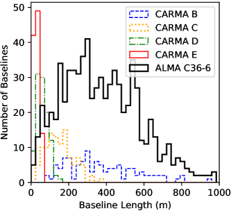
Figure 1.— Baseline length distributions for the four CARMA configurations and the ALMA configuration used for our observations. Each bin is 24m wide.

Table 5ALMA Sources

ID	Field	Position	Peak Flux	Total Flux	Deconvolved	RMS	Position
				Density	Size		Angle
	Ser-emb #	RA, Dec (ICRS)	(mJy beam-1)	(mJy)	(arcsec)	(mJy beam-1)	(degrees)
1	1	18:29:09.09 +00:31:30.9	92.64 (0.88)	125.37 (1.90)	0.24 x 0.14	0.20	98
2	2	18:29:52.53 +00:36:11.5	7.41 (0.30)	18.95 (1.05)	0.63 x 0.11	0.06	165
3	2	18:29:52.54 +00:36:10.3	0.97 (0.30)	0.96 (0.51)	-	0.06	-
4	2	18:29:52.40 +00:35:52.6	8.66 (0.31)	23.85 (1.12)	0.59 x 0.26	0.06	53
5	3	18:28:54.87 +00:29:52.0	9.10 (0.18)	10.54 (0.35)	0.15 x 0.09	0.07	151
6	4 (N)	18:29:59.94 +01:13:11.3	2.80 (0.11)	3.66 (0.24)	0.22 x 0.12	0.07	51
7	4 (N)	18:30:00.67 +01:13:00.1	3.16 (0.11)	3.50 (0.21)	0.13 x 0.07	0.07	68
8	4 (N)	18:30:00.73 +01:12:56.2	3.14 (0.11)	3.43 (0.20)	0.12 x 0.06	0.07	131
9	5	18:28:54.91 +00:18:32.3	7.85 (0.09)	10.08 (0.19)	0.19 x 0.12	0.07	162
10	6	18:29:49.80 +01:15:20.3	342.46 (5.35)	985.14 (20.05)	0.45 x 0.40	0.67	165
11	6	18:29:49.66 +01:15:21.1	29.33 (4.98)	119.72 (24.85)	0.68 x 0.45	0.67	88
12	7	18:28:54.06 +00:29:29.3	16.75 (1.02)	22.12 (2.16)	0.20 x 0.16	0.08	77
13	8	18:29:48.72 +01:16:55.5	15.19 (1.48)	37.28 (4.92)	0.48 x 0.29	0.13	69
14	8	18:29:48.09 +01:16:43.3	28.81 (1.51)	53.18 (4.04)	0.33 x 0.24	0.13	35
15	9	18:28:55.82 +00:29:44.3	3.34 (0.20)	5.07 (0.47)	0.29 x 0.17	0.07	99
16	9	18:28:55.77 +00:29:44.1	3.14 (0.21)	5.35 (0.52)	0.29 x 0.23	0.07	48
17	11 (W)	18:29:06.62 +00:30:33.9	30.77 (0.54)	57.20 (1.45)	0.30 x 0.28	0.14	87
18	11 (W)	18:29:06.77 +00:30:34.1	16.35 (0.52)	20.89 (1.08)	0.19 x 0.13	0.14	163
19	11 (W)	18:29:07.09 +00:30:43.0	3.03 (0.47)	2.49 (0.72)	-	0.14	-
20	15	18:29:54.30 +00:36:00.7	34.58 (0.53)	61.48 (1.40)	0.41 x 0.15	0.07	117
21	17	18:29:06.20 +00:30:43.0	41.48 (0.62)	97.87 (2.00)	0.38 x 0.35	0.12	138
22	17	18:29:05.61 +00:30:34.8	7.17 (0.58)	7.76 (1.07)	0.11 x 0.06	0.12	165

3. Reduced ALMA Maps and Source Identification

Maps of the Serpens protostars targeted by our ALMA observations were produced using the clean task in CASA 4.7.2. During self-calibration, all channels in each spectral window were averaged together to increase the SNR. The clean task was then run in multi-frequency synthesis mode to a threshold of 3$\sigma$ (measured by the RMS in an emission free region of each image) using Briggs weighting with robust=0.25 and a pixel size of 0.06″ to produce 60x60″ maps. All maps were primary beam corrected to a limiting response level of 0.1, corresponding to an image diameter of $40\arcsec$. After correction, the flux of point-like sources was measured by Gaussian fitting. Postage stamps from the resulting maps are shown in figures 2 and 3, while the corresponding Gaussian fits are provided in table 5. In each figure, YSOs previously identified by mid-IR Spitzer surveys (Dunham et al., 2015) are indicated by green pluses (Class 0, I, and Flat-Spectrum) and orange crosses (Class II and III).

While Enoch et al. (2011) only detected sources towards nine of the twelve Serpens fields surveyed, our observations find sources in every field owing to ALMA’s higher sensitivity (0.1 mJy vs the $>0.9$ mJy in the CARMA maps). Most sources are resolved by the 0.3″beam, and many are surrounded by extended structure which may in some cases be evidence of cavity walls sculpted by outflows. As the ALMA configuration used was selected to filter out spatial scales larger than $3.0$″, there is additional extended structure missing from our images. Ser-emb 4 (N) shows a clear example of this, as it is faint and marginally resolved out by ALMA, but is strongly detected (SNR $>20$) in CARMA maps made only with visibilities for scales $>4.1\arcsec$ (Enoch et al., 2011).

In comparisons to the locations of our sources with Spitzer YSOs, there is generally good correspondence, however, there are several sources detected in our 1.3 mm maps with no associated Spitzer source. Discussion of these sources and further descriptions of each ALMA map are given in the appendix.

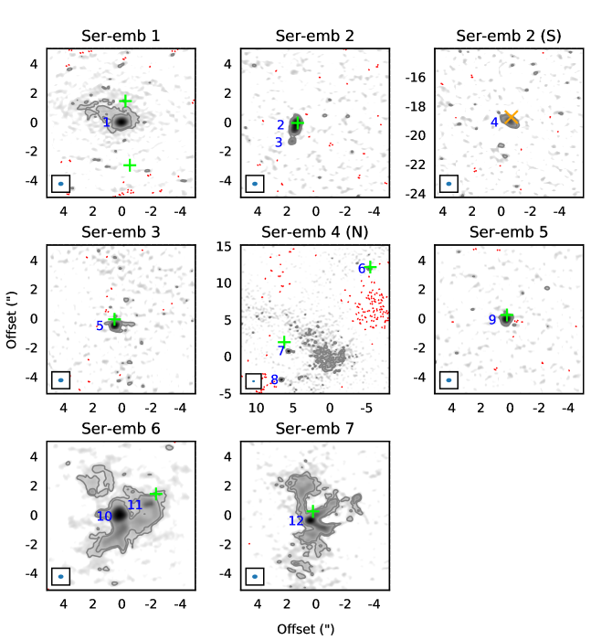
Figure 2.— Postage stamps from our ALMA maps of our Serpens Sample of deeply embedded protostars. Intensity is shown in negative greyscale with logarithmic scaling to highlight extended structure. The x and y axes correspond to the offset from the pointing center (table 2) of each map. Grey contours are shown at 3 and 5 times the RMS in each map, while dashed red contours are shown at -3 times the RMS. Blue numbers indicate the ID of the sources in each map which were fit by a Gaussian in table 5. YSOs previously identified by mid-IR Spitzer (Dunham et al., 2015) surveys are indicated by green pluses (Class 0+I and Flat Spectrum) and orange crosses (Class II and III). Each map is shown without primary beam correction for clearer flux scaling. Full maps from each pointing are provided in the appendix.

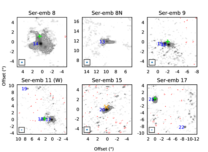
Figure 3.— Figure 2 cont.

4. Detecting Variability in Ideal Comparisons of Interferometer Observations

The smallest variation in flux of a source that can be robustly detected by comparing two interferometric observations depends upon the continuum RMS noise, the method used for calibrating and measuring flux, and how differences in spatial and spectral configurations are accounted for. The most ideal situation would be the comparison of observations made with the same telescope and identical setups, and thus here we compare our 2016 observations against themselves to find approximate lower limits on detectable flux variations, while leaving discussion of comparing different interferometer setups to section 5.

4.1. Continuum RMS Noise of Observations

Our 2016 ALMA observations were requested to reach a continuum RMS noise level of 0.1 mJy, defined as the RMS in an emission free region of a deconvolved (i.e. cleaned) continuum image. This RMS noise limit was intended to allow reaching a SNR $>50$ for our targets, where the SNR is defined as the ratio of peak flux to RMS noise. For our ALMA maps produced from the first scan, the achieved RMS noise (and the RMS as a percentage of the peak flux) is plotted against the peak flux for each source in figure 4. Many of our detected sources have an RMS noise greater than that expected (i.e., above $\sqrt{2}$ times the red curve), however, this can be readily explained by the reduced sensitivity of the ALMA dishes to sources near the edge of the field of view and the dynamic range limit of ALMA. Large open symbols in figure 4 account for the increased noise for sources nearer the edge of the field of view, while smaller filled symbols indicate the RMS noise level had every source been at the field center. Some sources still would lie significantly above the expected noise level even if they had been observed at the field center (small grey symbols). Here the noise is dominated by the dynamic range limit of ALMA due to a brighter source in the same field (green symbols). ALMA’s dynamic range limit describes the expected SNR for the brightest source in the field without self-calibration, and is nominally  100 for Band 6 observations (ALMA Cycle 3 Proposer’s Guide). We find through a fit to the expected noise behaviour for our observations after self-calibration (blue curve in figure 4.) that the dynamic range limit is $\sim 400$.

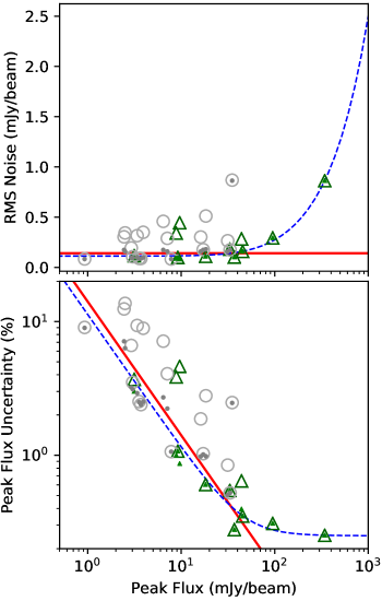
Figure 4.— Upper panel: Achieved RMS noise vs the peak flux for each source in the first scan of our ALMA observations. Lower panel: Same as upper panel, but with the % uncertainty in Peak Flux on the y axis, i.e., the RMS noise divided by the Peak Flux. Large open symbols represent measurements accounting for the increased noise due to the reduced sensitivity of the ALMA primary beam near the field edge, while small filled symbols use the RMS noise at the field center. Green triangles are the brightest sources in a given field, grey circles are from fields with a brighter source, which may cause ALMA to reach its dynamic range limit. The red line is $\sqrt{2}$ times the requested RMS noise of 0.1 mJy. The blue curve in the upper panel is an empirical fit to the brightest peaks with the RMS noise of the field center of the form $A=\sqrt{R^{2}+P^{2}/D^{2}}$, where $A$ and $R$ are the achieved and requested RMS, $P$ is the peak flux, and $D$ is the fitted dynamic range limit. The blue curve in the lower panel plots this function divided by Peak Flux, $A/P$.

4.2. Comparison of First and Second ALMA Scans

To estimate lower limits on detectable flux variations using only ALMA, we divided our visibility data for each field into its individual scans, then independently self-calibrated and imaged each scan using the same CASA clean parameters as those for the full data set in section 3. Integrated and peak fluxes were measured for each source by an elliptical Gaussian fit using CASA imfit. We also measured the integrated and peak flux in fixed regions of the sky enclosing each source (“Box Method”), typically a square 1-1.5″  in size. For this method, the uncertainty in the peak flux is the RMS noise, while that for the integrated flux is $\sqrt{N}$ times the RMS noise, where $N$ is the number of pixels in the region. The use of the Box Method for measuring flux is motivated by the large number of sources which are resolved and/or embedded in extended structure, and therefore not well described by a Gaussian model.

Regardless of how flux measurements are made on the images, direct comparisons between two ALMA observations will be limited by the nominal Band 6 flux calibration accuracy of $\sim$10% (Remijan et al., 2015). Poor flux calibration accuracy is a general issue with mm/sub-mm observing caused by the paucity of bright, stable point sources .

To sidestep this problem, we turn to relative flux calibration methods similar to those used in the JCMT Transient Survey (Mairs et al., 2017a), and apply them to both our predictions here and our comparison of ALMA and CARMA observations in section 5. We determine Relative Flux Calibration Factors (rFCFs) to bring the flux scale of the first scan into agreement with the second by fitting an average to the flux ratios between scans for bright sources ($>10$ mJy). We also separately find rFCFs for only the dim sources ($<10$ mJy or mJy/beam ) as a sanity check and to see what level of variability could be detected without bright sources. When fitting the average to determine the rFCF, each point is weighted by $\sigma^{-2}$, where $\sigma$ is the uncertainty in the ratio given by the errors added in quadrature of the flux measurements in the first and second scan. The overall uncertainty in the rFCF is given by the standard deviation of the ratios, again weighted by $\sigma^{-2}$. The ratios and rFCF fits for just the Box peak flux and Gaussian integrated flux are shown in figure 5, while table 6 summarizes all rFCF values. All of the rFCFs are consistent with 1, and most deviate by $\lesssim 0.01$, demonstrating that the ALMA calibration is extremely stable between scans on the $\sim 40$ minute timescale of our observations. The precision of rFCFs derived from integrated fluxes are typically lower than those derived from peak fluxes by a factor of 2-5, due to the larger relative uncertainties in integrated flux. The precision for rFCFs determined using Gaussian fits are lower than those using the peak/integrated Box flux because we assume flux measurements are independent between scans, yet many of our sources are poorly described by a Gaussians and thus have flux uncertainties dominated by the quality of fit. This causes the flux uncertainties to be correlated scan-to-scan, resulting in a larger rFCF uncertainty. The best rFCF precision is thus achieved using the Box peak flux (essentially the SNR), with a precision of 0.7% and 3.3% for bright and dim sources respectively. This is consistent with what would be expected from the inverse of the SNR for representative dim ($\sim 30$) and bright ($\gtrsim 100$) sources.

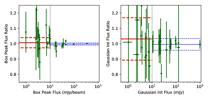
Figure 5.— Ratio between the second and first scans in peak flux estimated using a fixed region (box) on the sky and integrated flux estimated by a Gaussian fit. The average weighted by $\sigma^{-2}$ and the associated standard deviation are shown by the solid and dashed lines for dim sources ($<10$ mJy or mJy/beam ), and bright sources ($>10$ mJy or mJy/beam). The values of these averages are summarized in table 6

.

Table 6Relative Flux Calibration Factors (rFCFs) for ALMA data

rFCF Measurement Method	Dim	Bright
Box Peak Flux	1.006 (0.033)	0.998 (0.007)
Box Int Flux	0.990 (0.152)	0.997 (0.012)
Gaussian Peak Flux	1.012 (0.074)	1.002 (0.012)
Gaussian Int Flux	1.031 (0.138)	0.995 (0.038)

It should be emphasized that reaching sensitivity to low levels of variability requires both a precisely determined rFCF and high SNR flux measurement for an individual source. Table 7 summarizes the percentage change in flux we would be sensitive to at a $3\times$RMS level for a given rFCF and Flux percentage error (assuming that the Flux percentage error does not change between observations). Using the Box peak flux rFCFs, we are thus sensitive to variability at the $\sim 16\%$ level for representative dim sources (3 mJy; 3% flux error) and at the $\sim 4.8\%$ level for bright sources (10 mJy; 1% flux error).

Furthermore, it should be noted that since our observations were taken in a snapshot mode, the uv-coverage of each scan used in these comparisons is nearly identical. To estimate how small differences in uv-plane sampling might affect our sensitivity to variability, we conducted additional tests where a distinct subset of antennas was dropped at random from each scan, and rFCFs were calculated using the Box peak flux as described above. These tests were done removing 2, 4, or 8 of the 39 antennas from each scan, which is equivalent to having 89%, 78%, or 55% of visibilities from each scan at identical positions in the uv-plane. The resulting rFCF values remain consistent with 1.0, while the sensitivity to variability for a 10 mJy source with 2, 4, and 8 antennas randomly dropped respectively becomes 4.8% (unchanged), 5.6%, and 7.8%. This suggests that small differences in uv-plane sampling will not significantly affect our ability to detect variability. The general impact of larger differences in uv-plane sampling is discussed in depth in section 5.

Table 73$\times$RMS Percentage Variability detection Thresholds

Flux Err. (%)	rFCF Err. (%)
	0.3	0.5	1	3	5	10	20
0.3	1.6	2.0	3.3	9.1	15.1	30.0	60.0
0.5	2.3	2.6	3.7	9.2	15.1	30.1	60.0
1	4.3	4.5	5.2	9.9	15.6	30.3	60.1
3	12.8	12.8	13.1	15.6	19.7	32.6	61.3
5	21.2	21.3	21.4	23.0	26.0	36.7	63.6
10	42.4	42.5	42.5	43.4	45.0	52.0	73.5
20	84.9	84.9	84.9	85.3	86.2	90.0	103.9

5. Detecting Variability between Distinct Interferometric Observations with ALMA and CARMA

While the results of section 4 provide a lower limit for detections of variability in ideal conditions, they do not take into account many of the complications involved in comparing typical interferometric observations. These issues are caused by the inherent flexibility of interferometers, which typically have multiple array configurations for recovering structure over a range of spatial scales, and a variety of frequency bands and correlator modes for sampling different parts of the spectrum.

For comparing our ALMA and CARMA observations, we first attempt to address the problems caused by differences in array configuration in sections 5.1-5.3, and then turn to relative flux calibration methods for searching for variability in 5.4.

5.1. Impact of Differences in Spatial Configurations

Interferometers sample the complex visibility $V(u,v)$ of a source, a Fourier transform of it’s intensity distribution on the sky (ignoring effects of the primary beam) and a function of the spatial frequencies $u$ and $v$. The spatial frequencies sampled are determined by the projected lengths of the array’s baselines (in units of the observing $\lambda$) on the sky in the East-West ($u$) and North-South ($v$) directions. Since the projected baseline lengths and orientations change as the earth rotates, the $uv$-plane becomes better sampled over the course of observation, however, this implies that no two interferometric observations will recover exactly the same visibilities unless they observe with identical array configurations and observing schedules, from the same latitude, and at the same wavelength. Since the synthesized beam is simply the Fourier transform of the (weighted) visibility sampling function, this is equivalent to stating that two observations will not have the same beam unless subject to the above conditions.

While differences in $uv$-plane sampling are not a problem for imaging point sources, (which have a constant visibility amplitude over the $uv$-plane) images of resolved sources constructed by inverting $V(u,v)$ will contain varying amounts of flux depending on the $uv$-plane sampling. This issue is partly mitigated by algorithms used in imaging such as CLEAN, which effectively estimate $V(u,v)$ in un-sampled regions of the uv-plane by interpolating between samples, however, extrapolating to regions with no samples at all is extremely difficult. In particular, CLEAN has trouble in accurately extrapolating to the center of the $uv$-plane (where large spatial scales are measured), which is typically poorly sampled by interferometers because of a lack of short baselines.

An example is helpful in further illustrating how differences in $uv$-plane sampling can affect the recovered flux. Consider a point source embedded in extended structure observed by two different configurations of the same interferometer - the first with the antennas in a group compact enough to recover the largest spatial scales of the extended structure, and the second with the antennas spaced further apart, providing higher resolution but missing some of the extended structure. If images are produced for both observations and the flux of the point source is to be measured, the compact configuration image can be used to make a more accurate estimate of the point source flux by fitting for both the point source and the underlying larger scale structure.

To account for this bias, changes in the flux of this point source between the two observations should be measured using images constructed only using visibilities which measure similar spatial scales. There are several ways to accomplish this which we discuss in the following sections, including $uv$-plane matching of synthesized beams and simulated observations.

5.2. $uv$-plane Matching of ALMA and CARMA Synthesized Beams

To directly compare our ALMA and CARMA data for a given source, we first include only visibilities from each observation which sample a similar region of the $uv$-plane, in order to match the synthesized beam shapes as closely as possible. This requires some care, as a simple euclidean distance is not appropriate for comparing $uv$-plane separations between visibilities. The angular scale a visibility measures is the inverse of its euclidean distance from the $uv$-plane origin, and thus a given euclidean distance between two points near the origin is equivalent to a much larger change in angular scale than for the same distance between two points far from the origin. To avoid this problem, we instead use the euclidean distance between ALMA and CARMA visibilities as a fraction of the $uv$-distance to the CARMA visibility from the origin. Figure 6 shows in detail how this fractional distance is used for matching two fictional ALMA and CARMA data sets with an unrealistically large cutoff distance of $f_{\text{cut}}=0.4$.

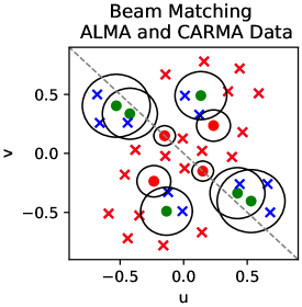
Figure 6.— Demonstration of how beams are matched for our observations using two fictitious data sets. ALMA and CARMA visibilities in the $uv$-plane are indicated by blue/red crosses and green/red disks respectively. Red disks and crosses are visibilities which will be removed from each data set by beam matching. The dashed grey line shows the inherent symmetry axis of the $uv$-plane. The black circles around each CARMA visibility indicate the cut-off distance for beam matching; if there are no samples from the ALMA data set within the cut-off distance (here, $f_{\text{cut}}=0.4$), the CARMA visibility in the original data set is removed. Any ALMA visibilities which do not fall within the cut-off distance to a CARMA visibility are also removed.

For comparisons of our observations, we wish to optimize the value of $f_{\text{cut}}$ by choosing it to match the beam dimensions as closely as possible (smaller $f_{\text{cut}}$) without removing so much data that the SNR drops severely (larger $f_{\text{cut}}$). Since the distribution of baselines for our ALMA configuration is essentially a superset of those for CARMA C (see figure 1), a useful value of $f_{\text{cut}}$ should mostly remove visibilities from the ALMA data while retaining as many from the (much lower SNR) CARMA data as possible. Figure 8 shows the distributions of nearest neighbours between a pair of ALMA and CARMA observations of the same Serpens source in units of fractional distance, from which a value of $f_{\text{cut}}$ of $\sim 0.25$ appears optimal. Since the $uv$-coverage is similar for all other pairs of observations, we use $f_{\text{cut}}=0.25$ in every comparison. Figure 7 shows an example of the $uv$-plane distributions before and after applying beam matching with $f_{\text{cut}}=0.25$ to a pair of ALMA and CARMA observations of the same source.

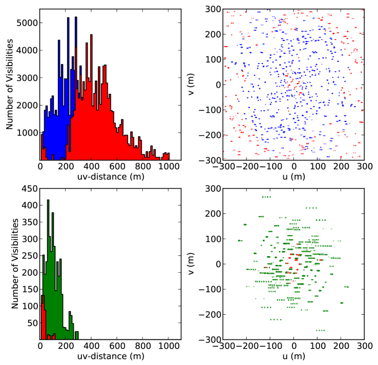
Figure 7.— Effect of applying beam matching with $f_{\text{cut}}=0.25$ on the $uv$-plane distributions of visibilities for CARMA Track C1.2 and our ALMA observations of Ser-emb 1. The top and bottom rows of panels shows the ALMA and CARMA distributions respectively, where red indicates visibilities removed by beam matching.

Once the visibility data from each observation to be compared are selected, preliminary maps are produced with the same parameters as we did for the full ALMA maps in section 3. In table 8, we compare the beam shapes before and after matching. While correspondence in the ALMA and CARMA synthesized beams has improved with their respective increase and decrease in size, CARMA’s beam is still typically $\sim 0.3\arcsec$ larger in either axis than ALMA’s. This can be attributed to differences in the $uv$-plane sampling density and weighting of the visibilities which $uv$-plane matching does not take into account. The sampling density of ALMA is significantly better than CARMA at all $uv$-distances, but is relatively skewed towards large $uv$-distance owing to the longer baselines. Furthermore, longer baseline tend to also have larger phase scatter from atmospheric fluctuations, resulting in a drop in visibility amplitude (Zauderer et al., 2016). These noisier visibilities are flagged or given a lower weight during calibration, resulting in less sensitivity on longer baselines. This affects the data from CARMA more than that from ALMA because of the poorer observing conditions at the CARMA site. To correct for these effects, we also apply a $uv$-taper to each ALMA observation when imaging the data (last column of table 8). The taper used is equivalent to smoothing by a circular Gaussian kernel with FWHM equal to the major axis of the corresponding matched CARMA beam, and improves the agreement in beam shapes to within $\sim 0.1\arcsec$ or better for both axes.

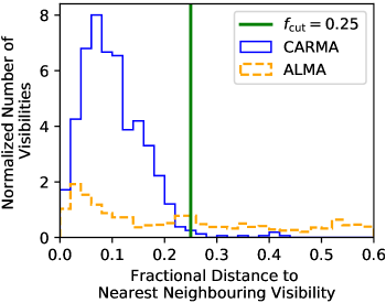
Figure 8.— Normalized histograms of nearest neighbouring visibilities (in the other data set) for our ALMA and the CARMA track C1.5 observations of Ser-emb 6. The bin size is 0.02. The fractional distance cut-off $f_{\text{cut}}$ used for beam matching of all ALMA and CARMA observations is shown by the vertical line.

Table 8Beam Shapes Before and After $uv$-plane Matching

Matching Track	Unmatched (″)			Matched (″)
	CARMA	ALMA		CARMA	ALMA	ALMA + $uv$ taper
C1.2	1.73 x 1.40	0.35 x 0.27		1.16 x 1.00	0.82 x 0.65	1.19 x 1.02
C1.5	1.72 x 1.62			1.46 x 1.21	1.12 x 0.95	1.53 x 1.38
C1.8	1.67 x 1.43			1.30 x 0.85	0.92 x 0.54	1.32 x 1.10
C2.3	1.54 x 1.39			1.02 x 0.82	0.69 x 0.49	1.04 x 0.87

Note. — Beam sizes given are the FWHM of the major and minor axes.

5.3. Simulated Re-observations of ALMA sources with CARMA

Simulated observations provide another means of comparing our ALMA and CARMA data while taking into account differences in $uv$-plane sampling. Typically, simulated observations are used to predict what an interferometer will see with a particular array configuration and observing setup given a model of the true sky brightness. The model is often the result of a numerical simulation or an image from another telescope. In our case, we use the maps derived from our ALMA observations in section 3 with the residuals subtracted as models, and then use CASA’s simobserve task to simulate what CARMA would see had it re-observed the same sources in a identical manner as it did in 2007, and compare against the beam matched CARMA maps from section 5.2. A similar approach was successfully used by Hunter et al. (2017) for detecting variability between SMA and ALMA observations of the massive protocluster NGC 6334-I, albeit with a readily detectable factor of $\sim 4$ change in flux.

In order to realistically simulate the conditions under which the original CARMA data were taken, the same array configuration, correlator setup, observing schedule, and data flagging must be used. For our simulations, we ensure the $uv$-coverage is the same by extracting the exact positions of the CARMA antennas from the data and applying the same observing schedule, integration time, and flagging. For the spectral setup, we simply use a single 2.8 GHz wide spectral window centred on the ALMA observing frequency (227 GHz), rather than the exact parameters in table 3 due to limitations of the CASA simobserve task. While the observing frequencies of ALMA and CARMA are slightly different, changes in the flux should be small and mitigated by relative flux calibration (see discussion in section 6). Finally, we do not add any noise to the simulated visibilities, as we are only modelling differences in $uv$-coverage that would affect measurement of variability, and not attempting to determine sensitivities for a CARMA to CARMA comparison.

From the simulated visibilities, maps are produced using the same parameters as those in section 3, but only including visibilities more than 30m from the $uv$-plane origin. We apply this $uv$-plane cut as a good approximation to the effects of beam matching on the CARMA data. The simulated and $uv$-plane matched beam shapes are compared against each other in table 5.3. As was similarly the case for beam matching, differences in beam shape of $\sim 0.2\arcsec$ remain, however, this likely arises from variations in the visibility weighting not modelled in the simulations, as the $uv$-coverages of the beam matched and simulated observations are nearly identical. To correct for this, a $uv$-taper corresponding to the CARMA matched beam is added to each simulated image when cleaning as was done for beam matching.

Table 9CARMA Beam Shapes In Real and Simulated Observations

Track	Matched (″)	Simulated (″)	Sim. + Taper (″)
C1.2	1.16 x 1.00	1.08 x 0.71	1.18 x 0.95
C1.5	1.46 x 1.21	1.23 x 1.06	1.44 x 1.25
C1.8	1.30 x 0.85	1.09 x 0.75	1.24 x 1.05
C2.3	1.02 x 0.82	0.89 x 0.77	1.02 x 0.92

Note. — Beam sizes given are the FWHM of the major and minor axes.

5.4. Relative Flux Calibration Factors and Variability of Sources

With differences in beam shapes minimized, we can reliably measure fluxes of sources common to both observations and attempt searches for variability. As discussed in section 4, direct comparisons are limited by the accuracy of the absolute flux calibration for each telescope, $\sim$10% for ALMA in Band 6 (ALMA Cycle 3 Technical Handbook) and $\sim$20% for the CARMA observations (Enoch et al., 2011). We therefore calculate rFCFs by fitting an average to the ratio of ALMA to CARMA Box peak fluxes, and use them to convert the CARMA maps to the ALMA flux scale for both methods of beam comparison. Specifically, rFCFs for $uv$-plane beam matching (section 5.2) are fit to the ratio of fluxes in pairs of beam matched CARMA and ALMA maps (specific to each CARMA track), while rFCFs for simulated re-observation (section 5.3) are fit to the ratio of fluxes between the ALMA maps with simulated re-observation by CARMA and the corresponding beam matched CARMA track. The resulting rFCFs for CARMA tracks C1.2, C1.5, and C2.3 and the standard deviation between them, $\sigma_{\text{rFCF}}$, are shown in table 10. Within the uncertainties given, differences in the flux calibration factors across beam comparison methods are consistent with each other and reach a similar level of precision. Further comparison of the two methods and discussion of which may be best suited to future variability studies is given in section 6.

In table 10, a rFCF can not be properly calculated for CARMA track C1.8, as there is only a single observable source in common with the ALMA observations. Relative variability can thus not be detected, and the rFCF given is just the ratio of the brightness of this source (Ser-emb 1, ID 1). This ratio for C1.8 is consistent with the $\sigma_{\text{rFCF}}$ found for the other three tracks.

Given that there is only one ALMA flux calibration for every image, $\sigma_{\text{rFCF}}$ is effectively an estimate of the CARMA absolute flux calibration accuracy. We find $\sigma_{\text{rFCF}}$ to be $\sim 40\%$ for either beam comparison method compared to the $\sim 15\%$ expected from the nominal CARMA absolute flux accuracy. Some of this loss of accuracy is probably caused by the low SNR of the sources used for relative calibration, and some might be attributed to poorer-than-average weather during several of the CARMA tracks. Since $\sigma_{\text{rFCF}}$ was only determined from 3 tracks however, it is not particularly robust.

For tracks C1.2, C1.5, and C2.3, the rFCFs may be useful for measuring variability, but are still not particularly well constrained due to there only being 3-4 sources per track in common with our ALMA observations (see table 4). Determining accurate rFCFs is further hampered by the low signal to noise detections of many of the sources in the CARMA tracks, with most detected with a SNR of 5-15 and the brightest at a SNR of 30. For tracks C1.2 and C1.5, the relative flux calibration is good to the $\sim 10\%$ level, while for the fainter sources compared in C2.3, the relative flux calibration is accurate to $\sim 50\%$, no better than the $\sim 18\%$ uncertainty due to the combined absolute flux calibration of ALMA and CARMA.

Tables 11-13 compare the fluxes in each epoch for each track after application of the rFCFs. Here, the detection $\sigma$ is the the percent difference between the fluxes divided by it’s uncertainty. No source is seen to vary above $\gtrsim 1\sigma$ by either the beam matching or simulated observation analysis. The uncertainty in the percent difference for each source implies our ability to detect variability at a 3$\sigma$ level is $\sim 24-60\%$ for tracks C1.2 and C1.5 and $\sim 75-180\%$ for track C2.3, depending on the brightness of the source in question. These detection thresholds are much larger than those expected from comparison of multiple epochs of ALMA data in section 4, emphasizing the need for large numbers of bright sources to achieve good sensitivity to variability.

Table 10Relative Flux Calibration Factors

Beam Comparison Method	CARMA Track Name				$\sigma_{\text{rFCF}}$
	C1.2	C1.5	C1.8	C2.3
Beam Matching	1.32 (0.09)	0.74 (0.11)	1.02 (0.06)	1.85 (0.54)	0.45
Simulated Re-Observation	1.15 (0.14)	0.64 (0.04)	0.93 (0.05)	1.56 (0.49)	0.37

Table 11Variability of Sources, CARMA Track C1.2

Beam Comparison Method	ID	Beam Matched & Scaled	Equivalent ALMA Flux	Percent Difference	Detection $\sigma$
		CARMA Flux
		(mJy beam-1)	(mJy beam-1)
$uv$-plane Beam Matching	1	114.07 (16.31)	125.33 (0.69)	9.88 (15.72)	0.63
	10	876.38 (67.20)	847.56 (5.47)	-3.29 (7.44)	0.44
	11	121.95 (26.22)	113.91 (5.48)	-6.59 (20.58)	0.32
Simulated Re-Observation	1	99.44 (17.58)	114.10 (0.02)	14.75 (20.28)	0.73
	10	763.97 (98.70)	773.80 (0.21)	1.29 (13.09)	0.10
	11	106.31 (25.39)	89.26 (0.21)	-16.03 (20.05)	0.80

.

Table 12Variability of Sources, CARMA Track C1.5

Beam Comparison Method	ID	Beam Matched & Scaled	Equivalent ALMA Flux	Percent Difference	Detection $\sigma$
		CARMA Flux
		(mJy beam-1)	(mJy beam-1)
$uv$-plane Beam Matching	1	155.20 (25.47)	129.80 (0.85)	-16.36 (13.74)	1.19
	10	966.61 (153.03)	919.68 (5.59)	-4.86 (15.07)	0.32
	11	187.46 (34.39)	227.24 (5.59)	21.22 (22.44)	0.95
Simulated Re-Observation	1	134.89 (12.20)	120.83 (0.01)	-10.43 (8.10)	1.29
	10	840.12 (66.76)	860.11 (0.20)	2.38 (8.14)	0.29
	11	162.93 (19.90)	176.04 (0.20)	8.05 (13.19)	0.61

.

Table 13Variability of Sources, CARMA Track C2.3

Beam Comparison Method	ID	Beam Matched & Scaled	Equivalent ALMA Flux	Percent Difference	Detection $\sigma$
		CARMA Flux
		(mJy beam-1)	(mJy beam-1)
$uv$-plane Beam Matching	17	38.28 (14.75)	53.95 (0.23)	40.92 (54.29)	0.75
	18	34.14 (13.89)	21.38 (0.24)	-37.37 (25.50)	1.47
	20	68.42 (21.34)	57.52 (0.22)	-15.93 (26.22)	0.61
	21	78.10 (26.51)	87.77 (0.30)	12.38 (38.14)	0.32
Simulated Re-Observation	17	32.21 (12.95)	47.75 (0.11)	48.25 (59.59)	0.81
	18	28.72 (12.14)	17.29 (0.11)	-39.79 (25.46)	1.56
	20	57.56 (19.13)	52.05 (0.01)	-9.58 (30.05)	0.32
	21	65.71 (23.54)	66.45 (0.15)	1.13 (36.23)	0.03

.

6. Discussion & Conclusion

Given that large bursts in deeply embedded protostars have only been detected a handful of times, the lack of flux variations above the detection limits of $\sim 24-180\%$ in our Serpens sample is not unexpected. The only source in our sample with prior evidence of variability is Ser-emb 6 (SMM1), which is rising by $\sim 5\%/yr$ in the Transient Survey (Johnstone et al., 2018). Extrapolating over the 9 year difference between the ALMA and CARMA epochs and assuming we would see a similar change (ignoring differences in spatial scale and observing frequency) suggests we might have expected a 45% increase in flux, which would be at or above a 3$\sigma$ detection level for this source (see tables 11-13). Given that we expect variability at the scales of the accretion disk, we would expect the signature of variability could be stronger than 45% in the comparisons of ALMA and CARMA observations than in the Transient Survey where changes in flux are diluted by envelope material in the JCMT beam. Instead, the results of section 5.4 are consistent with no change, suggesting that the rise in brightness of SMM1 seen by the Transient survey (between March 2016 and June 2017) may have only began recently.

The greatest limitations in our comparisons are imposed by the relatively low signal to noise of the CARMA data and the small numbers of objects common to both the ALMA and CARMA observations available for relative flux calibration, which hinder the determination of precise and statistically robust rFCFs. Our comparisons of the ALMA data against itself however, suggest that if a second epoch with similar resolution and sensitivity were obtained, variations at the level of a few percent could be detected for sources with a SNR $>100$, (those brighter than 10 mJy) about 14 in our sample. Moreover, ALMA’s excellent sensitivity makes such an observation efficient - our snapshot observation reached a sensitivity of $100\mu$ Jy in 40 minutes, compared to the sensitivity of the CARMA maps of 1-3 mJy (Enoch et al., 2011), achieved by combining data from over 20 nights of observations over three years. As the JCMT Transient Survey finds 10% of protostars varying at $\sim|5|\%$yr^-1, (including includes SMM1 (Ser-emb 6), an object also in our sample) a second epoch of ALMA observations with a similar array configuration and integration time would likely find robust low level variability in at least 1-2 objects. As the signature of variability is likely being diluted by the JCMT beam at the scales of the envelope it probes, it is possible that even more detections could be made.

The results of section 5 suggest $uv$-plane beam matching and simulated re-observations are similarly effective in terms of their sensitivity to variability, resulting rFCF precision, and ability to match the main lobes of the clean beams. While $uv$-plane beam matching is much simpler to implement, simulated re-observations can apply identical $uv$-plane sampling from one epoch of observations to the the other by carefully taking into account the array setup. Both methods could possibly be improved by taking into account differences in visibility weighting between two epochs in a more precise way than the $uv$-taper we have chosen to use. Future work should also focus on generalizing these methods to compare $>2$ epochs of observations, so reliable light curves can eventually be produced.

Some techniques not explored in this work could also improve the chances of finding variability. We have not taken into account small differences in observing frequency between our 233 GHz ALMA observations and 230 GHz CARMA observations. Assuming a spectral index for optically thin dust of 2.5, a 3 GHz difference in frequency might see a difference in flux of 3.3%. Our relative flux calibration should remove frequency dependent differences in dust emission in an average sense, but does not take into account variations in dust properties between objects. This can be corrected for by fitting a spectral index for each while performing deconvolution. This could be useful for comparing archival observations, which likely have been done with different observing frequencies as well as telescope configurations. Another unexplored technique is the possibility of measuring fluxes by fitting models of each source directly to the visibility data in the uv-plane. The structure of each source could be approximated using simple multi-component models, e.g. a point source embedded in a low-amplitude flat or Gaussian function to represent extended emission. This approach would have the advantages of comparing the visibility data in a more direct way (i.e., without deconvolution, which itself is essentially a model fitting process) and permitting all of the data from different uv-plane samplings to be used instead of being culled or down-weighted, and it could still be used in conjunction with a relative calibration scheme. Disadvantages of this approach would include the modelling uncertainty in choice of functions used to represent each source, and the necessity for a careful analysis of the visibility weights in order to ensure robust uncertainties in the measured flux.

Future work on identifying variability in deeply embedded protostars is underway. A Cycle 6 ALMA proposal for 4 epochs of ACA-only Band 7 observations of variables in Serpens identified by the JCMT Transient survey has been accepted (PI: Logan Francis, project code 2018.1.00917.S). These observations will complement results from the contemporaneous Transient Survey by observing at 850 $\mu$m with a resolution of 3.8″(compared to the 14.6″resolution of the JCMT), sufficient to reach the scale of the inner envelopes ($\sim 1500$AU) of protostars in Serpens.

7. Acknowledgements

We would like to thank Helen Kirk, Sümeyye Suri, Laura Perez, John Carpenter, and Gerald Scheiven for their support with ALMA and CARMA data reduction and useful insights on this project. We would also like to thank the anonymous referee for their helpful comments on this paper.

Doug Johnstone is supported by the National Research Council of Canada and by an NSERC Discovery Grant. The National Radio Astronomy Observatory is a facility of the National Science Foundation operated under agreement by the Associated Universities, Inc. ALMA is a partnership of ESO (representing its member states), NSF (USA) and NINS (Japan), together with NRC (Canada) and NSC and ASIAA (Taiwan) and KASI (Republic of Korea), in cooperation with the Republic of Chile. The Joint ALMA Observatory is operated by ESO, AUI/ NRAO and NAOJ. This paper makes use of the following ALMA data: ADS/JAO.ALMA#2015.1.00310.S,

This work makes use of the following software: The Common Astronomy Software Applications (CASA) package (McMullin et al., 2007b), CASA analysisUtils, Python version 2.7, astropy (Astropy Collaboration et al., 2013), aplpy (Robitaille & Bressert, 2012), and matplotlib (Hunter, 2007).

Appendix A Discussion of Individual Fields in Serpens Main

The Serpens Main cluster has been extensively surveyed at a variety of wavelengths and resolutions over the past 30 years. Our ALMA observations provide some of the highest resolution and most sensitive maps of deeply embedded protostars in the cluster to date. In many of our fields, we are thus able to resolve single sources at the scale of the accretion disks, uncover significant extended structure, and identify previously unknown faint sources. Here, we discuss each field in the context of past and recent observations, and compare the positions of our sources with YSOs identified in the Spitzer “cores to disks” (c2d) and “Gould Belt” (GB) surveys (Dunham et al., 2015). Table 14 lists the properties of all c2d/GB YSOs in our fields associated with our mm sources in table 5.

The Ser-emb objects targeted by our ALMA and the earlier CARMA observations (Enoch et al., 2011) were originally defined from large scale Bolocam 1.1 mm and Spitzer mid-IR surveys, and classified according to their bolometric temperature (Enoch et al., 2009). Most of our targets lie in two dense clusters: the northern Main Cluster (Ser-emb 4, 6, 8) and the southern Cluster B (Ser-emb 3, 7, 9, 11, 17). Three sources are relatively isolated (Ser-emb 2, 5, 15) from either cluster. An overview of the region showing these clusters and the locations of the targeted embedded sources can be found in figure 1 of Enoch et al. (2011).

Our figures 9-11 show the continuum maps with the full field of view for each of our ALMA pointings, and indicate the positions and IDs of c2d/GB YSOs by green pluses (Class 0+1, Flat Spectrum) and orange crosses (Class II). Red squares show the location of the postage-stamp views in figures 2 and 3.

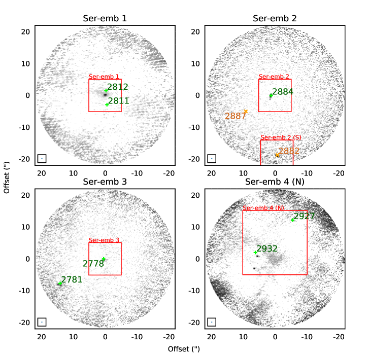
Figure 9.— Full maps of our ALMA observations of Serpens protostars. Red squares indicate the field of view for the postage stamps in figures 2 and 3. The maps are shown with primary beam correction to indicate ALMA’s field of view.

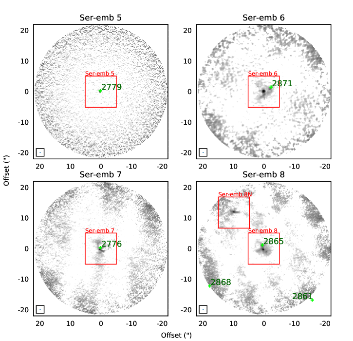
Figure 10.— As figure 9.

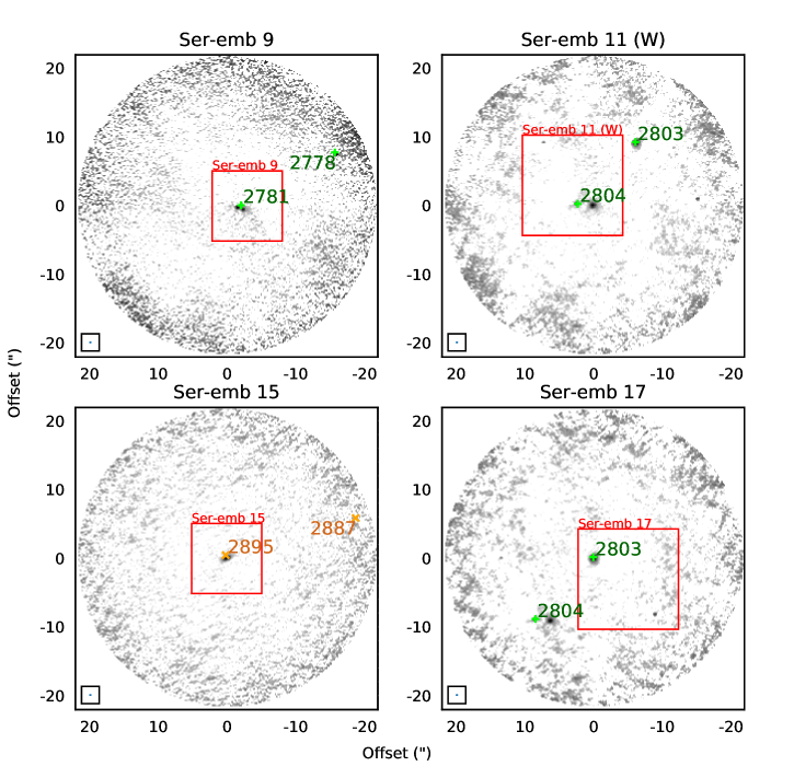
Figure 11.— As figure 9.

Table 14Properties of the Serpens c2d+GB YSOs

	Spitzer		Extinction Corrected				Associated
	Source Name	$A_{\rm V}$		$T_{bol}$′	$L_{bol}$′		ALMA Source	Field
Index	(SSTc2d or SSTgb +)	(mag)	$\alpha^{\prime}$	(K)	(L⊙)	Class	ID	Ser-emb #
2776	J182854.0+002930	9.6	1.15	69	8.80	0+I	12	Ser-emb 7
2778	J182854.8+002952	9.6	1.60	51	6.60	0+I	5	Ser-emb 3,9
2779	J182854.9+001832	9.6	0.68	150	0.14	0+I	9	Ser-emb 5
2781	J182855.7+002944	9.6	1.65	26	1.60	0+I	15,16	Ser-emb 3,9
2803	J182906.2+003043	9.6	1.33	67	10.00	0+I	21	Ser-emb 11(W), 17
2804	J182906.7+003034	9.6	1.40	83	5.40	0+I	17,18	Ser-emb 11(W), 17
2811	J182909.0+003128	9.6	0.07	420	0.03	Flat	-	Ser-emb 1
2812	J182909.0+003132	9.6	2.13	36	4.20	0+I	1	Ser-emb 1
2865	J182948.1+011644	9.6	1.11	30	14.00	0+I	14	Ser-emb 8
2871	J182949.6+011521	9.6	2.53	13	69.00	0+I	11	Ser-emb 6
2882	J182952.3+003553	40.0	-1.55	2400	17.0	II	4	Ser-emb 2
2884	J182952.5+003611	9.6	0.54	68	1.90	0+I	2,3	Ser-emb 2
2887	J182953.0+003606	9.6	-0.35	890	0.58	II	-	Ser-emb 2, 15
2895	J182954.3+003601	9.6	-0.33	59	1.70	II	20	Ser-emb 15
2927	J182959.9+011311	9.6	2.20	120	7.00	0+I	6	Ser-emb 4 (N)
2932	J183000.7+011301	9.6	1.52	29	8.10	0+I	7	Ser-emb 4 (N)

Note. — This table adapted from table 2 of Dunham et al. (2015).

A.1. Ser-emb 1

Ser-emb 1 is seen in our ALMA maps as a bright (100 mJy beam^-1) point-like source (ID 1) surrounded by faint, marginally detected ($3\sigma$) emission extending to the North-East. This extended structure is likely a component of the bright emission visible on $\sim 10\arcsec$ scales in the short-spacing CARMA maps of Enoch et al. (2011), which our ALMA observations are mostly insensitive to.

Ser-emb 1 is the Class 0 source with the lowest bolometric temperature (39K) in Serpens Main (Enoch et al., 2009), suggesting it is also the least evolved. A N-S oriented bi-polar jet likely originating from Ser-emb 1 is seen in 2.122 $\mu$m H₂ emission (Djupvik et al., 2016). N-S oriented CO outflows are also seen emanating directly from the source in CO (J = 2 $\rightarrow$ 1) Hull et al. (2014).

Two c2d/GB YSOs (Dunham et al., 2015) are found within a few arcseconds of source 1. The closer YSO, 2812, has a lower $T_{bol}$(36 K), similar to that found by Enoch et al. (2009). YSO 2811 is a warmer (420 K) source with no corresponding mm emission visible in our ALMA maps, which is perhaps unsurprising given its very low bolometric luminosity (0.03 L_⊙) and more evolved flat spectrum classification.

Ser-emb 1 is coincident (to within $\sim$ 2″) with a 3.6 cm radio continuum source detected by the VLA, which may result from thermal free-free emission in shocks (Djupvik et al., 2006).

A.2. Ser-emb 2

Three compact, faint ($<10$mJy beam^-1) sources (IDs 2-4) are found in the maps of ALMA Ser-emb 2. Enoch et al. (2011) detected these sources only at a $5\sigma$ level in preliminary 110 GHz maps, but did not follow up with 230 GHz (1.3 mm) observations as was done for the other Ser-emb objects due to their faintness.

The central sources in our map correspond to the location of Ser-emb 2 and consist of a disk-like ($\sim 275$ AU major axis) component (ID 2) connected to a point source (ID 3) by a small ridge of emission. The c2d/GB YSO 2884 is coincident with source 2 and has $\mbox{$T_{bol}$}=68$ K.

The source at the southern edge of the field (ID 4) also appears to be a compact resolved disk ($\sim 257$ AU major axis), and is associated with c2d/GB YSO 2882. This class II YSO is more evolved and the hottest in our sample, with a $\mbox{$T_{bol}$}=2400$ K. It is also the most optically extincted at $A_{\text{V}}=40$, compared to the $A_{\text{V}}=9.6$ for all other YSOs in these fields.

Gould Belt YSO 2887 appears within the field, but with no corresponding mm emission, possibly because of its more evolved Class II status and lower luminosity ($\mbox{$L_{bol}$}=0.58L_{\odot}$). This YSO is also seen on the edge of the adjacent Ser-emb 15 field.

A.3. Ser-emb 3 and 9

Ser-emb 3 and 9 are located close enough together ($\sim 15\arcsec$ apart) that they are both seen in two of our ALMA pointings. Neither were mapped at 230 GHz by Enoch et al. (2011) due to the lack of clear detections in 110 GHz maps.

Ser-emb 3 is seen as a faint $\sim 9$ mJy beam^-1 point source (ID 5) associated with the c2d/GB YSO 2778, a $\mbox{$T_{bol}$}=51$ K class 0+I object.

Ser-emb 9 appears as a tight pair of $\sim 9$ mJy beam^-1 peaks (IDs 15, 16) separated by just $\sim 0.5\arcsec/215$ AU and embedded in fainter emission. It is associated with the Gould Belt YSO 2781, a Class 0+1 source with $\mbox{$T_{bol}$}=26$ K. Ser-emb 9 is also seen associated with a 3.6 cm radio to within 1″ (Djupvik et al., 2006).

A.4. Ser-emb 4 (N)

ALMA observations of this field detect three faint ($<3$ mJy/beam) point sources (IDs 6, 7, 8). In the CARMA observations, three regions of extended emission are detected and named Ser-emb 4 S, E, and N. Ser-emb 4 N is the brightest component of this CARMA source, but due to its extended nature, our ALMA configuration barely detects it at the field center. Our ALMA observations find the Eastern-most point source (Source 8) is coincident with Ser-emb 4 E, but do not detect the fainter envelope around the source seen by CARMA. Ser-emb 4 S is similarly undetected.

The point source East of Ser-emb 4 N (Source 7) is associated with c2d/GB YSO 2932, a class 0+I source with $\mbox{$T_{bol}$}=28$ K. Since no compact mm emission or mid-IR c2d/GB sources are found at the positions of Ser-emb N and S, these sources are likely pre-stellar in nature.

The Northern-most point source (Source 6) in this field is identified as Ser-emb 19, a class I with $\mbox{$T_{bol}$}=129$ K in Enoch et al. (2009). It is also associated with Gould Belt 2927, a Class 0+I found to have a similar $\mbox{$T_{bol}$}=120$ K.

A.5. Ser-emb 5

A single 7.8 mJy beam^-1 point source (ID 9) is found at the field center of our ALMA observations. Enoch et al. (2011) similarly detect a faint point source, and suggest the object is the precursor to a brown dwarf or in a very low state of accretion due to its low luminosity ($\mbox{$L_{bol}$}=0.4\mbox{L${}_{\odot}$}$). The Class 0+I c2d/GB YSO 2779 is found at the position of this source, and has $\mbox{$T_{bol}$}=129$ K and a low luminosity ($\mbox{$L_{bol}$}=0.14L_{\odot}$.

A.6. Ser-emb 6

Ser-emb 6 [also known as Serpens FIRS 1 (Harvey et al., 1984) and SMM 1 (Casali et al., 1993)] is the brightest Class 0 source in Serpens Main and one of the most extensively studied. CARMA observations of the source found an extended envelope surrounding two resolved sources. In our ALMA observations, we see two extremely bright resolved sources ($\sim 1000$ mJy beam^-1, ID 10 and $\sim 100$ mJy beam^-1, ID 11) surrounded by complex extended structure. For consistency with other high-resolution ALMA observations of this object [e.g Hull et al. (2016)], we will refer to the bright central source as SMM1-a and the relatively fainter western source as SMM1-b.

SMM1-a and b are associated with several jets and outflows. Hull et al. (2016) find high velocity $\sim 80$ km/s CO ($J=2\rightarrow 1$) jets emanating from SMM1-a and b. They interpret the C-shaped extended structure around SMM1-a as walls of a cavity carved by precession of the jet. The same cavity is also seen in free-free emission from VLA observations, which Hull et al. (2016) suggest to be caused by ionization of gas in shocks at the cavity walls. Polarization measurements with ALMA suggest that the jets are playing a role in shaping the local magnetic field (Hull et al., 2017a). Lower velocity ($\sim 10-20$ km/s) wide angle outflows are also seen in the CO ($J=2\rightarrow 1$) emission around the high velocity jets Hull et al. (2014, 2017a). Mid-IR Spitzer observations also find jets in H₂ and various atomic emission lines (e.g. [FeII]), however, interpreting which source is driving each outflow is complicated by the complexity of the outflows and lower Spitzer resolution (Dionatos et al., 2014).

We find one c2d/GB YSO, 2871, coincident with SMM1-b, however, given that the beam size of Spitzer ranges 2.5″to 40″depending on the instrument and wavelength, flux from the brighter SMM1-a is almost certainly a large contribution if not dominating contribution to the YSO’s determined properties. Its low temperature ($\mbox{$T_{bol}$}=13$ K) and high luminosity ($\mbox{$L_{bol}$}=69L_{\odot}$) agree well with the classification of Ser-emb 6 as a bright Class 0 source by Enoch et al. (2009). The coincidence of 2871 with source SMM1-a rather than b could also indicate that a is fainter at mid-IR wavelengths, but higher resolution observations would be needed to confirm this.

SMM1 is the only source in our sample which is confirmed to be variable at sub-mm wavelengths. It has been rising in brightness by $\sim 5\%$yr^-1 in the first 18 months of the JCMT Transient Survey from December 2017 to June 2018 (Johnstone et al., 2018) and by $\sim 2\%$yr^-1 from 2012 to 2016 in comparisons of archival Gould Belt Survey and Transient survey data (Mairs et al., 2017b). Future epochs of ALMA observations should be able to determine if SMM1-a or b is the source of the rising brightness provided this trend continues.

A.7. Ser-emb 7

Ser-emb 7 is detected in the ALMA observations as a $\sim 17$ mJy beam^-1 point source (ID 12) surrounded by complex and filamentary extended structure of $\sim 1000$ AU in size. This is suggestive of a fragmenting disk or interaction with outflows. No outflows in Spitzer maps of the Cluster B region are linked to the structure surrounding Ser-emb 7, however, the source has yet to be observed at high resolution in CO or another tracer. Ser-emb 7 and extended structure are also seen in the CARMA observations, where maps constructed from large scale visibilities show an envelope extending $\sim 15\arcsec$ to the South of the source which is resolved out by our ALMA configuration.

The Class 0+I c2d/GB YSO 2776 is associated with Ser-emb 7. It is found to have a ($\mbox{$T_{bol}$}=60$K), similar to the ($\mbox{$T_{bol}$}=58$K) for Ser-emb 7 in Enoch et al. (2009). Ser-emb 7 is also associated with a 3.6 cm radio continuum source Djupvik et al. (2006) 5″ to the North.

A.8. Ser-emb 8/S68N

Ser-emb 8 [Also known as S68N (McMullin et al., 1994) and SMM 9 Casali et al. (1993)] is detected in our ALMA maps as a $\sim 30$ mJy beam^-1 point source (ID 14) surrounded by knotty extended emission. Another point source (ID 13) surrounded by extended structure is also detected to the North-East in our observations, here-after referred to as Ser-emb 8N. In the CARMA observations, large scale emission joins together the Ser-emb 8N and 8 in large scale maps. Both 8 and 8N power molecular outflows observed in SiO ($J=5\rightarrow 4$) extending SE-NE (Hull et al., 2014). Maps of this source in polarized dust emission find that magnetic fields at the 100-1000 AU scales are weak and randomly oriented, suggesting turbulence plays a dominant role in establishing the field morphology at these scales Hull et al. (2017b).

Greene et al. (2018) have recently analysed a near-IR spectrum of Ser-emb 8 and detected features of the stellar photosphere (the first such detection and analysis for a Class 0 protostar), finding a photosphere temperature similar to pre-main-sequence stars, but with a lower surface gravity and larger stellar radius.

One class 0+1 Gould Belt YSO, 2865 is associated with Ser-emb 8, lying about 2″to the North of the bright central peak. No c2d/GB YSOs are associated with Ser-emb 8N, suggesting that it is too faint and/or deeply embedded to be detected at mid-IR wavelengths.

A.9. Ser-emb 11 (W) and 17

Ser-emb 11 and 17 are located $\sim 10\arcsec$ apart, and are thus seen in two of our ALMA pointings. 5 sources are found in both pointings (IDs 17-22). In both the ALMA and CARMA observations, Ser-emb 11 and 17 are detected and Ser-emb 11 is resolved into two components (IDs 17, 18). Both the targeted objects are bright, with peak fluxes of $\sim 31$ and $\sim 42$  mJy beam^-1 for Ser-emb 11 (W) (ID 17 )and 17 (ID 21) respectively. Some extended emission is seen around Ser-emb 11 and 17 in the ALMA maps.

Two previously unrecognized point sources (IDs 19, 22) are also found in the field. Both are faint, with a peak flux of $\sim 3$ (ID 19) and $\sim 7$ (ID 22)  mJy beam^-1. Comparing the positions of these faint sources with the large scale CARMA maps in figure 3 of Enoch et al. (2011), there is some extended emission around the brighter $\sim 7$ mJy beam^-1 source directly West of Ser-emb 11 (W), but none around the faint source North-East of Ser-emb 11 (W). The faintness of these sources makes them qualitatively similar to Ser-emb 5, and thus they might also be proto-Brown dwarfs or objects in very low level accretion states. However, no Gould Belt YSOs are associated with either object, nor can we rule out the possibility we may be seeing a background sub-mm galaxy, making such an interpretation insecure.

Ser-emb 11 and 17 have both been suggested as candidate driving sources for outflows seen in 2.122 $\mu$m H₂ by Spitzer Djupvik et al. (2016). Outflows are also seen closer to each source in CO ($J=2\rightarrow 1$) Hull et al. (2014).

Ser-emb 11 E (ID 18) is associated with c2d/GB YSO 2804, a $\mbox{$T_{bol}$}=67$K source, and Ser-emb 17 is similarly associated with YSO 2803, a $\mbox{$T_{bol}$}=73$K source. Similar bolometric temperatures are found by Enoch et al. (2009), who place both objects in Class I. Ser-emb 11 is additionally associated with a 3.6 cm continuum source less than $\sim 1$″  away Djupvik et al. (2006).

A.10. Ser-emb 15

Ser-emb 15 is detected in both the ALMA and CARMA observations, and a disk-like ($\sim 126$ AU major axis) source (ID 20) with a $\sim 35$ mJy beam^-1 peak is seen in our ALMA observations.

Ser-emb 15 is associated with c2d/GB YSO 2895, a marginal class II ($\alpha^{\prime}=-0.33$) source with $\mbox{$T_{bol}$}=120$K, the warmest of our targeted Ser-emb objects. Enoch et al. (2009) place Ser-emb 15 in Class I with $\mbox{$T_{bol}$}=100$K, which is likely a more appropriate categorization of the object given the extended disk seen in these ALMA observations.

References

- Armitage et al. (2001) Armitage, P. J., Livio, M., & Pringle, J. E. 2001, MNRAS, 324, 705
- Astropy Collaboration et al. (2013) Astropy Collaboration, Robitaille, T. P., Tollerud, E. J., et al. 2013, A&A, 558, A33
- Audard et al. (2014) Audard, M., Ábrahám, P., Dunham, M. M., et al. 2014, Protostars and Planets VI, 387
- Bae et al. (2014) Bae, J., Hartmann, L., Zhu, Z., & Nelson, R. P. 2014, ApJ, 795, 61
- Bonnell & Bastien (1992) Bonnell, I., & Bastien, P. 1992, ApJ, 401, L31
- Casali et al. (1993) Casali, M. M., Eiroa, C., & Duncan, W. D. 1993, A&A, 275, 195
- Cha & Nayakshin (2011) Cha, S.-H., & Nayakshin, S. 2011, MNRAS, 415, 3319
- Chen et al. (1995) Chen, H., Myers, P. C., Ladd, E. F., & Wood, D. O. S. 1995, ApJ, 445, 377
- Costigan et al. (2014) Costigan, G., Vink, J. S., Scholz, A., Ray, T., & Testi, L. 2014, MNRAS, 440, 3444
- Dempsey et al. (2013) Dempsey, J. T., Friberg, P., Jenness, T., et al. 2013, MNRAS, 430, 2534
- Dionatos et al. (2014) Dionatos, O., Jørgensen, J. K., Teixeira, P. S., Güdel, M., & Bergin, E. 2014, A&A, 563, A28
- Djupvik et al. (2006) Djupvik, A. A., André, P., Bontemps, S., et al. 2006, A&A, 458, 789
- Djupvik et al. (2016) Djupvik, A. A., Liimets, T., Zinnecker, H., et al. 2016, A&A, 587, A75
- Dunham et al. (2010) Dunham, M. M., Evans, II, N. J., Terebey, S., Dullemond, C. P., & Young, C. H. 2010, ApJ, 710, 470
- Dunham et al. (2014) Dunham, M. M., Stutz, A. M., Allen, L. E., et al. 2014, Protostars and Planets VI, 195
- Dunham et al. (2015) Dunham, M. M., Allen, L. E., Evans, II, N. J., et al. 2015, ApJS, 220, 11
- Enoch et al. (2009) Enoch, M. L., Evans, II, N. J., Sargent, A. I., & Glenn, J. 2009, ApJ, 692, 973
- Enoch et al. (2011) Enoch, M. L., Corder, S., Duchêne, G., et al. 2011, ApJS, 195, 21
- Greene et al. (2018) Greene, T. P., Gully-Santiago, M. A., & Barsony, M. 2018, ApJ, 862, 85
- Greene et al. (1994) Greene, T. P., Wilking, B. A., Andre, P., Young, E. T., & Lada, C. J. 1994, ApJ, 434, 614
- Hartmann et al. (2016) Hartmann, L., Herczeg, G., & Calvet, N. 2016, ARA&A, 54, 135
- Hartmann & Kenyon (1996) Hartmann, L., & Kenyon, S. J. 1996, ARA&A, 34, 207
- Harvey et al. (1984) Harvey, P. M., Wilking, B. A., & Joy, M. 1984, ApJ, 278, 156
- Herbig (1977) Herbig, G. H. 1977, ApJ, 217, 693
- Herbig (2008) —. 2008, AJ, 135, 637
- Herczeg et al. (2017) Herczeg, G. J., Johnstone, D., Mairs, S., et al. 2017, ApJ, 849, 43
- Hodapp (1999) Hodapp, K. W. 1999, AJ, 118, 1338
- Hodapp et al. (2012) Hodapp, K. W., Chini, R., Watermann, R., & Lemke, R. 2012, ApJ, 744, 56
- Holland et al. (2013) Holland, W. S., Bintley, D., Chapin, E. L., et al. 2013, MNRAS, 430, 2513
- Hull et al. (2014) Hull, C. L. H., Plambeck, R. L., Kwon, W., et al. 2014, ApJS, 213, 13
- Hull et al. (2016) Hull, C. L. H., Girart, J. M., Kristensen, L. E., et al. 2016, ApJ, 823, L27
- Hull et al. (2017a) Hull, C. L. H., Girart, J. M., Tychoniec, Ł., et al. 2017a, ApJ, 847, 92
- Hull et al. (2017b) Hull, C. L. H., Mocz, P., Burkhart, B., et al. 2017b, ApJ, 842, L9
- Hunter (2007) Hunter, J. D. 2007, Computing in Science and Engineering, 9, 90
- Hunter et al. (2006) Hunter, T. R., Brogan, C. L., Megeath, S. T., et al. 2006, ApJ, 649, 888
- Hunter et al. (2017) Hunter, T. R., Brogan, C. L., MacLeod, G., et al. 2017, ApJ, 837, L29
- Jensen & Haugbølle (2018) Jensen, S. S., & Haugbølle, T. 2018, MNRAS, 474, 1176
- Johnstone et al. (2013) Johnstone, D., Hendricks, B., Herczeg, G. J., & Bruderer, S. 2013, ApJ, 765, 133
- Johnstone et al. (2018) Johnstone, D., Herczeg, G. J., Mairs, S., et al. 2018, ApJ, 854, 31
- Kenyon et al. (1990) Kenyon, S. J., Hartmann, L. W., Strom, K. M., & Strom, S. E. 1990, AJ, 99, 869
- Liu et al. (2017) Liu, H. B., Dunham, M. M., Pascucci, I., et al. 2017, ArXiv e-prints, arXiv:1710.08686
- Lodato & Clarke (2004) Lodato, G., & Clarke, C. J. 2004, MNRAS, 353, 841
- Machida et al. (2011) Machida, M. N., Inutsuka, S.-i., & Matsumoto, T. 2011, ApJ, 729, 42
- Mairs et al. (2017a) Mairs, S., Lane, J., Johnstone, D., et al. 2017a, ApJ, 843, 55
- Mairs et al. (2017b) Mairs, S., Johnstone, D., Kirk, H., et al. 2017b, ApJ, 849, 107
- McKee & Offner (2011) McKee, C. F., & Offner, S. R. R. 2011, in IAU Symposium, Vol. 270, Computational Star Formation, ed. J. Alves, B. G. Elmegreen, J. M. Girart, & V. Trimble, 73–80
- McMullin et al. (1994) McMullin, J. P., Mundy, L. G., Wilking, B. A., Hezel, T., & Blake, G. A. 1994, ApJ, 424, 222
- McMullin et al. (2007a) McMullin, J. P., Waters, B., Schiebel, D., Young, W., & Golap, K. 2007a, in Astronomical Society of the Pacific Conference Series, Vol. 376, Astronomical Data Analysis Software and Systems XVI, ed. R. A. Shaw, F. Hill, & D. J. Bell, 127
- McMullin et al. (2007b) McMullin, J. P., Waters, B., Schiebel, D., Young, W., & Golap, K. 2007b, in Astronomical Society of the Pacific Conference Series, Vol. 376, Astronomical Data Analysis Software and Systems XVI, ed. R. A. Shaw, F. Hill, & D. J. Bell, 127
- Myers & Ladd (1993) Myers, P. C., & Ladd, E. F. 1993, ApJ, 413, L47
- Nayakshin & Lodato (2012) Nayakshin, S., & Lodato, G. 2012, MNRAS, 426, 70
- Ortiz-León et al. (2017) Ortiz-León, G. N., Dzib, S. A., Kounkel, M. A., et al. 2017, ApJ, 834, 143
- Pfalzner et al. (2008) Pfalzner, S., Tackenberg, J., & Steinhausen, M. 2008, A&A, 487, L45
- Plunkett et al. (2015) Plunkett, A. L., Arce, H. G., Mardones, D., et al. 2015, Nature, 527, 70
- Rab et al. (2017) Rab, C., Elbakyan, V., Vorobyov, E., et al. 2017, A&A, 604, A15
- Reipurth (1990) Reipurth, B. 1990, in IAU Symposium, Vol. 137, Flare Stars in Star Clusters, Associations and the Solar Vicinity, ed. L. V. Mirzoian, B. R. Pettersen, & M. K. Tsvetkov, 229–251
- Remijan et al. (2015) Remijan, A., Adams, M., Eiji, A., & Andreani, P. 2015, ALMA Technical Handbook Cycle 3
- Robitaille & Bressert (2012) Robitaille, T., & Bressert, E. 2012, APLpy: Astronomical Plotting Library in Python, Astrophysics Source Code Library, ascl:1208.017
- Safron et al. (2015) Safron, E. J., Fischer, W. J., Megeath, S. T., et al. 2015, ApJ, 800, L5
- Sault et al. (1995) Sault, R. J., Teuben, P. J., & Wright, M. C. H. 1995, in Astronomical Society of the Pacific Conference Series, Vol. 77, Astronomical Data Analysis Software and Systems IV, ed. R. A. Shaw, H. E. Payne, & J. J. E. Hayes, 433
- Shu et al. (1987) Shu, F. H., Adams, F. C., & Lizano, S. 1987, ARA&A, 25, 23
- Simon et al. (2011) Simon, J. B., Hawley, J. F., & Beckwith, K. 2011, ApJ, 730, 94
- Taquet et al. (2016) Taquet, V., Wirström, E. S., & Charnley, S. B. 2016, ApJ, 821, 46
- Tassis & Mouschovias (2005) Tassis, K., & Mouschovias, T. C. 2005, ApJ, 618, 783
- Venuti et al. (2015) Venuti, L., Bouvier, J., Irwin, J., et al. 2015, A&A, 581, A66
- Vorobyov & Basu (2005) Vorobyov, E. I., & Basu, S. 2005, ApJ, 633, L137
- Vorobyov & Basu (2006) —. 2006, ApJ, 650, 956
- Vorobyov & Basu (2010) —. 2010, ApJ, 719, 1896
- Yoo et al. (2017) Yoo, H., Lee, J.-E., Mairs, S., et al. 2017, ApJ, 849, 69
- Zauderer et al. (2016) Zauderer, B. A., Bolatto, A. D., Vogel, S. N., et al. 2016, AJ, 151, 18
- Zhu et al. (2009a) Zhu, Z., Hartmann, L., & Gammie, C. 2009a, ApJ, 694, 1045
- Zhu et al. (2010) —. 2010, ApJ, 713, 1143
- Zhu et al. (2009b) Zhu, Z., Hartmann, L., Gammie, C., & McKinney, J. C. 2009b, ApJ, 701, 620