Forecasting Intra-Hour Imbalances
in Electric Power Systems

Abstract

Keeping the electricity production in balance with the actual demand is becoming a difficult and expensive task in spite of an involvement of experienced human operators. This is due to the increasing complexity of the electric power grid system with the intermittent renewable production as one of the contributors. A beforehand information about an occurring imbalance can help the transmission system operator to adjust the production plans, and thus ensure a high security of supply by reducing the use of costly balancing reserves, and consequently reduce undesirable fluctuations of the 50 Hz power system frequency. In this paper, we introduce the relatively new problem of an intra-hour imbalance forecasting for the transmission system operator (TSO). We focus on the use case of the Norwegian TSO, Statnett. We present a complementary imbalance forecasting tool that is able to support the TSO in determining the trend of future imbalances, and show the potential to proactively alleviate imbalances with a higher accuracy compared to the contemporary solution.

Introduction

The electrical power system is a highly complex system. One of the main reasons is the need for instantaneous balancing of supply and demand in any synchronous power system. The Nordic power system (consisting of the countries Norway, Sweden, Finland and Denmark) is no different. Additionally, it is undergoing a period of significant changes driven by the developments in the infrastructure and consumer behaviour (?). The volumes of intermittent renewable capacity has increased rapidly over the past decade, driven by a mix of environmental regulations and subsidies, and cost reduction. Furthermore, consumers of power are increasingly generating their own power. The increased volatility in production and demand resulting from these developments represent a significant challenge to the operation of power systems.

Also following the liberalisation of the Nordic power market in the 1990s (?), many of the tasks related to coordinating the supply and demand have been given to the market through the creation of the Nord Pool, a Nordic market for electric power exchange. In this market place, Nordic market actors exchange bids and offers and agree on the future production and delivery of physical power (?). Nevertheless, because of structural limitations in the market (mainly the time resolution being limited to hours) and the uncertainty associated with both generation and demand, there will always be a need for a transmission system operator (TSO) to handle instantaneous imbalances (i.e. differences between demand and supply) within the operating hour. As imbalances ultimately result in frequency deviations in the synchronous power system, managing these imbalances is a key in ensuring a stable and secure power supply.

Figure 1: A two hours ahead imbalance prediction with prediction intervals.

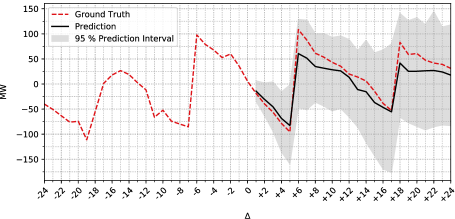
The TSOs work tightly together (e.g. Statnett with their Nordic counterparts such as Svenska Kraftnät, Energinet and Fingrid) to mitigate imbalances. Their toolbox for managing imbalances can be dived into the following categories:

• Preventive measures. These are measurements that are taken several hours before the operating hour, but after the market has determined the supply and demand. The TSO can then approximate the upcoming imbalances based on the supply and demand scheduled on an hourly resolution, and their intra-hour load forecast. The results of this approximation are presented in a so called Planning Table. Typically this results in smoothing out big hourly shifts in the scheduled production since the demand normally does not follow strict hourly patterns (?).

• Operational measures. There are three types of balancing reserves that can be activated within the operation hour usually in the given order:

  • Frequency Containment Reserves (FCR) which is a built-in flexibility in the power system resulting from requirements that the TSO has set for all generators providing power to the system.

  • Automatic Frequency Restoration Reserves (aFRR) which are automatically activated by the TSO and has a response time of maximum 2 minutes.

  • Manual Frequency Restoration Reserves (mFRR) which can be ordered by the TSO manually by communication with large power producers and which is set to have a response time of maximum 15 minutes.

In brief, the tools that are available for Statnett and other Nordic TSOs vary in terms of activation time, response time, magnitude of availability and cost. As a balancing strategy, Statnett uses mFRR both retrospectively (to free FCR and aFRR volumes that have been activated due to an occurred imbalance) and proactively (to mitigate upcoming imbalances). The objective is to minimize the use of expensive and limited FCR and aFRR, and thereby ensuring a high security of supply (?). In order to do so, Statnett relies on a human experience and the aforementioned Planning Table, which provides forecasts for the upcoming imbalances in the next two hours.

In essence, Planning Table is a prediction tool that takes the scheduled production from the market, and subtracts a 5-minute granularity demand (load) forecasts to calculate the upcoming imbalance. Unfortunately, the quality of the forecast provided by Planning Table is limited. Arguably, this is because it relies greatly on the assumptions that the market is in balance on an hourly granularity, that the generators produce the power without deviations from the plan, and that the demand prediction is accurate. This lack of an effective tool for forecasting upcoming market imbalances makes it hard to proactively manage imbalances with manual reserves, which in turn makes more use of the expensive and limited aFRR and FCR. As a result, it becomes difficult for the TSO reaching their KPI (Key Performance Indicator) in terms of frequency quality (i.e. minutes of frequency deviations in the past years) and experience increasing costs of balancing (?). This, coupled with the fact that published literature on forecasting system imbalance volumes is very limited, indicates great room for improvement (?), and is the main motivation behind this research.

In order to mitigate imbalances proactively and effectively, an improved or complementary forecasting tool would be of a great benefit to TSOs like Statnett. Such a tool would additionally implement some of the expert knowledge, and thus lessen the burden of the human experts, improve the decisions and the robustness of the power system, together with reduction of the costs for balancing.

In this work, we present a complementary forecasting solution giving the TSO information about the most likely trend of imbalances within the next two hours. Additionally, it is beneficial to have an information about the reliability of predictions especially in use cases where human experts are involved in the process of decision making. For this reason, the aforementioned imbalance predictions are accompanied with prediction intervals. By applying quantile forest regression on feature engineered data, our solution outperforms a proxy of Statnett’s contemporary forecasting solution, i.e. a more accurate representation of the Planning Table.

Problem Definition

We define the imbalances as a time series with 5-minute granularity, where each value represents an average imbalance of the past five minutes. The objective is to predict the imbalances two hours ahead. Formally, in a market area $\alpha$ and at time $t$, our objective is to predict 24 future imbalances $I_{\alpha,t+\Delta}$, where $\Delta\in\langle 1,24\rangle$, alternatively annotated as $\boldsymbol{I_{\alpha,t}}=(I_{\alpha,t+1},...,I_{\alpha,t+24})$. Imbalance predictions are denoted with $\hat{}$, i.e. $\hat{I}_{\alpha,t+\Delta}$ or $\boldsymbol{\hat{I}_{\alpha,t}}$. The goal is to minimize the difference between the predicted imbalance $\hat{I}_{\alpha,t+\Delta}$ and actual imbalance $I_{\alpha,t+\Delta}$. Additionally, each imbalance prediction $\hat{I}_{\alpha,t+\Delta}$ shall be accompanied with prediction interval $PI_{\alpha,t+\Delta}$ which is an estimate of an interval where an observed imbalance, i.e. $I_{\alpha,t+\Delta}$, will lie with a certain probability. In this work, $\alpha$ is one of the five market areas (labeled as $NO1$, $NO2$, $NO3$, $NO4$ and $NO5$) into which Norway is currently divided.

A key aspect is the definition of what precisely a single imbalance value represents. Since all imbalance managing measures share the purpose of reducing the imbalance, the imbalance itself varies with respect to which point in time it is measured. As the target model is intended to be an operational decision support tool for activating operational measurements, the imbalance is defined as the imbalance measured after preventive measures is taken, but before any operational measures have affected the imbalance. The imbalance is measured in megawatts (MW) and is commonly referred to as Area Control Error Open Loop (ACE OL). This definition ensures that the balancing measures (taken based on the predictions) do not affect the imbalances. Worth underlining is also that imbalance (ACE OL) can be computed only retrospectively at the end of the period of interest, as it essentially is determined by subtracting the actual operational measures from the actual observed imbalance (so called Area Control Error, or ACE). Additionally, the preventive measures are subtracted from ACE OL as they are planned ahead and known prior the prediction time (?).

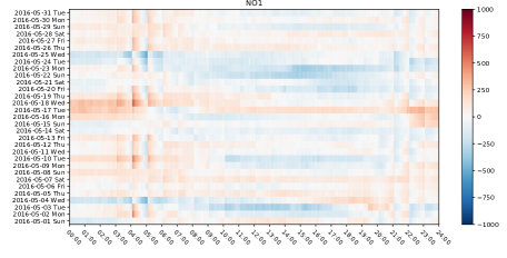
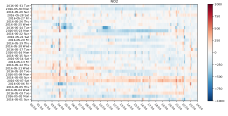
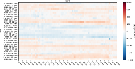
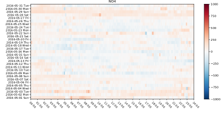
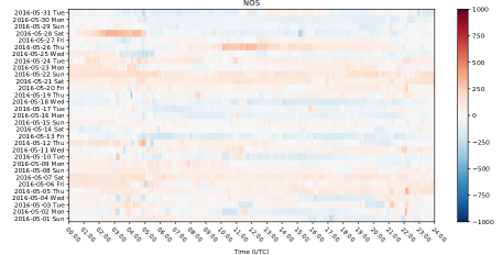
Figure 2 visualizes in a great detail the heterogeneous character of the pre-processed imbalances in the market areas within the same timespan (i.e. May 2016). Apparent is a strong correlation over time and differences between the areas. Notice the sudden changes in imbalance at the beginning of hours (e.g. in area NO1 at 3, 4 and 5 o’clock in the morning). This is due to the aforementioned hourly resolution of the planned production contrary to the abrupt intra-hour changes of the demand, even though possibly matching the hourly average of the production.

Related Work

To the best of our knowledge, only a handful of publications (?; ?; ?) are dealing with the power system imbalance forecasting, which gives a hint about the novelty of the topic. In comparison, a large number of publications deal, e.g., with the short-term load forecasting, prediction of market prices, and analysis of the impacts of increasing penetration of intermittent renewable sources. The following provides a brief overview of the three publications dealing with power system imbalance predictions.

The first publication (?) discusses and shows the limitations and insufficiency of richly applied but basic forecasting techniques such as ARIMA and exponential smoothing, because of the non-periodic, non-stationary and noisy character of imbalance time-series. Instead, the contemporary state-of-the-art artificial neural networks (ANN) are applied to uncover the non-linearity and irregularity of the data, and predict the daily imbalance medians. Presented are improvements compared to methods based on a linear regression, and the fact that none of the neural networks provided optimal predictions for all market conditions is discussed. Two use cases were evaluated: prediction of daily medians with three months training and one month testing window, and prediction of six values for each day with four week training and one week testing window. The following predictor variables were employed: demand forecast, demand forecast error, accepted bid volumes, accepted offer volumes, forward trades, gate closure imbalance volume, accepted offers and bids, imbalance prices and day of the week. However, it is not clear whether historical imbalances were utilized as one of the input features of the models.

The second publication (?) investigates the most important predictors contributing to accurate forecasts. The impact of multiple exogenous variables was analyzed by applying autocorrelation analysis. The exogenous variables were grouped into three classes: demand variables, supply variables, and market participants’ behaviour. One of the outcomes of the analysis is that variables of maximum two hours delay provide sufficient predictive power. However, we should be aware of the fact that autocorrelation is the linear dependence of a variable. The proposed model does not aim to predict imbalances accurately, instead, its objective is to map the future imbalance into one of five proposed intervals. The input variables have undergone similar discretization. The discretized dataset is used in a customized linear-regression-based model for forecasting intra-hour (with one minute granularity) imbalances. The model takes into account the exogenous variables and is being compared to the ARIMA based benchmark. Unfortunately, the current state-of-the-art modelling approaches do not seem to be exploited in this work.

Figure 2: Imbalances in the Norwegian market areas in May 2016.

The third publication (?) is dedicated to hourly imbalance predictions using random forest regression. Similarly to previous works, a broad range of influencing variables are taken into account. The listed variables may be grouped into demand forecast, wind forecast, temperature, bid volume in day-ahead market, day-ahead market price, energy volume auctioned in phase 2 of technical constraints and its price, reserves. The final model is trained with only eight-day dataset, and evaluated on the consequent ninth day. Multiple variants of feature sets were compared of their predictive performance. Model incorporating all features performed best, however, with a small margin. The work also presents a variable analysis predominantly exploring linear dependencies. However, it is not clear how the 24 target imbalances were predicted using random forests. It is worth noting that historical imbalances were not included in the feature set.

Incorporating the exogenous variables is an important research direction, and all of the above mentioned works have this in common. Their incorporation of influencing variables is related to several factors, including demand forecasts, market prices, planned production, weather observations and forecasts.

Of the aforementioned works, only the work by ? (?) copes with the problem of our interest, i.e. short-term power imbalance forecasting. Still, the aims of our solution are slightly different. The proposed solution should not replace the contemporary tool, Planning Table, but rather act as a complementing tool enhancing the judgment of the human experts. This is also due to existing constraints regarding the available data sources (as described in the Dataset section). Another important distinction to the mentioned works is that our solution provides prediction intervals, in addition to point predictions of imbalances.

Forecasting Intra-Hour Imbalances

This section describes the selected modelling approach, i.e. quantile regression forests (?), and the experimental setting producing the presented results.

The quantile regression forests (QRF) is a generalization of the random forests (?), a sound and widely applied ensemble learning method. Random forests (RF) provide point predictions in the form of conditional mean $E(Y|X=x)$, where $Y$ is the target variable and $X$ the predictor variable. QRF extends RF with the ability to generate prediction intervals as an intrinsic part of the model, thus allowing to assess the reliability of the predictions. Given $X=x$, the prediction interval $\mathcal{Q}_{p}(x)$ expresses that a new observation Y will lie with a certain probability ($p$) within an interval given by the lower quantile $Q_{l}$ and upper quantile $Q_{u}$. For example, a 95 % prediction interval is given by

$$\mathcal{Q}_{.95}(x)=[Q_{.025}(x),Q_{.975}(x)].$$

The $q$-quantile is then defined as

$$Q_{q}(x)=\inf\{y:P(Y\leq y|X=x)\geq q\}.$$

In RF (and QRF), the conditional mean $E(Y|X=x)$ is approximated as a weighted mean over the observations of the target variable $Y$. Similarly in QRF, the conditional distribution function $P(Y\leq y|X=x)$, defined as $E(1_{\{Y\leq y\}}|X=x)$, is approximated by weighted mean over the observations of $1_{\{Y\leq y\}}$. Therefore, each leaf of each tree stores also the observed target variables $Y$ besides their average.

The prediction of the 24 future imbalances is treated as an univariate prediction problem. This means that for each of the 24 predicted imbalance values, an independent model is trained. The imbalances are predicted for each price area separately. This results in 120 models in the given five market prices areas.

Through an empirical testing of training set sizes ranging from 3 to 18 months, the training sets of size at least 12 months manifested considerable performance gains. Greater training set sizes did not show evidence of diminishing performance. Therefore, the training set used in this paper consists of one year of data. The 12 months training set size was chosen also with regards of the test set size, allowing us to analyze the performance throughout the year. Also through empirical testing we have selected 1 month as a retraining interval, i.e. once per month a new model is trained with the preceding 12 months as training set. Note, however, that it is beyond the scope of this paper to present the empirical results for selecting the sizes of training set and test set.

Through an exhaustive hyper-parameter search with the focus on mean squared error (MSE), we were able to select hyper-parameters for each of the predicted imbalance values ($I_{\alpha,t+\Delta}$). However, as the gains were not significant, we selected one hyper-parameter set applied across all experiments. Here, the key hyper-parameters are 100 estimators (with minimum leaf size set to ten observations), each trained on bootstrapped data retaining a subset of 70 % randomly selected features. In our experiments, MSE was used as the splitting criterion.

Easy maintenance, i.e. retraining and adjustments in features, plays a key role when selecting the model type. RF type of models are known for their non-sensitiveness to overfitting and noise, and our empirical testing has also shown a small sensitivity to changes in HPs, i.e. small changes in the HPs do not lead to considerably different results. It is worth noting that QRF had a decisive influence on the model selection.

Dataset

This section describes the available data (defining the scope and limitations of this work), and the dataset used for training and testing of the proposed models. Consequently, we clarify the definition of an imbalance, a key aspect of the problem definition.

We base this work on a dataset provided by Statnett, which contains two years of imbalance data from 2015 to 2016. The dataset individually covers the five Norwegian market areas (pricing areas), recalling that the focus is on predicting imbalances in each market area separately. We will refer to the market areas as NO1, NO2, NO3, NO4 and NO5. The imbalance data is a time series made up by continuous timestamped values with a 5-minute granularity, where each value represent the average imbalance across the past 5 minutes ending at the timestamp. For each market area, the dataset comprises roughly 210K data points, in total.

The imbalance can be decomposed into three main contributing factors: error of the consumption forecast, deviations from the production plan, and deviations from the HVDC plan (i.e. planned import and export of the power). Here we ignore unforeseen events, such as failures in the electrical power grid, as another contributing factor. Each of the factors is further under influence of exogenous variables such as weather and human activity. Unfortunately, we were not able to decompose and utilize the imbalance contributors, due to the absence of the data. For this reason, we limit the scope of this work to following types of variables: historical imbalances, temporal features (including solar elevation), market prices, planned HVDC flows, production plans, and forecasts and observations of the temperature, wind and river flows.

The final dataset is a result of an exhaustive manual feature engineering (partly involving human experts from Statnett and Svenska Kraftnät) and feature selection process. We have evaluated the top-N features retrieved by the feature importance ranking of the RF. Additionally, aware of the feature importance diffusion of correlated features, multiple manually created (using previous results, the domain expertise and logical reasoning) feature subsets were evaluated. However, due to space constraints of this paper, we only present the final and simplest version of the utilized dataset. The final feature set, acting as predictor variables ($X$) in our model, has exhibited greatest gains in terms of predictive performance. The key features were dramatically reduced to the following: 24 past imbalances ($I_{\alpha,t-\delta}$, where $\delta\in\langle 1,24\rangle$) represented as relative values to $I_{\alpha,t+0}$, $I_{\alpha,t+0}$ (as an absolute value), and temporal features (month, day of the week, hour, minute, sine and cosine representation of the previously listed, holiday flag, and solar elevation). The prediction targets are also imbalance values relative to $I_{\alpha,t+0}$.

Figure 3: Plots of cumulative errors over time $t$ for each market area $\alpha$ and prediction target $t+\Delta$ in the year 2016. Due to space restrictions only results of $\Delta\in\langle 1,13\rangle$ are presented. The Planning Table benchmark is available only for a subset of data, i.e. for $\Delta\in\langle 1,7\rangle$ from March to September 2016.

Experimental Results

The predictions were evaluated on the period from January to December 2016. Each model was trained on 12 calendar months, and evaluated on the subsequent calendar month. This results into a set of 12 prediction sets times 24 predicted variables (two hours of imbalances) times 5 market areas.

For point predictions, we calculate the mean squared error (MSE) and the mean absolute error (MAE) to measure the accuracy. To evaluate the prediction intervals, we calculate the coverage probability (CP), which is essentially the probability that the future (observed) imbalances will lie within the constructed prediction intervals, and is given by

$$CP=\frac{1}{N}\sum_{i=1}^{N}c_{i}\quad\text{where}\quad c_{i}=\begin{cases}1&\text{if}\ y_{i}\in\mathcal{Q}_{p}(x_{i});\\ 0&\text{otherwise},\end{cases}$$

where $N$ is the total number of predictions, $y_{i}$ is an observed value and $\mathcal{Q}(x_{i})$ is the prediction interval. The 95 % prediction intervals were evaluated.

Two benchmarks are provided for the point predictions. The first benchmark, referenced as Naive, is a predictor assuming imbalances to be identical to previous week’s. The second benchmark, referenced as Planning Table, is a more accurate proxy of the Planning Table. This is due to missing consumption forecasts being replaced by actual consumption. Note that the Planning Table benchmark is available only for $\Delta\in\langle 1,7\rangle$ from March to September 2016.

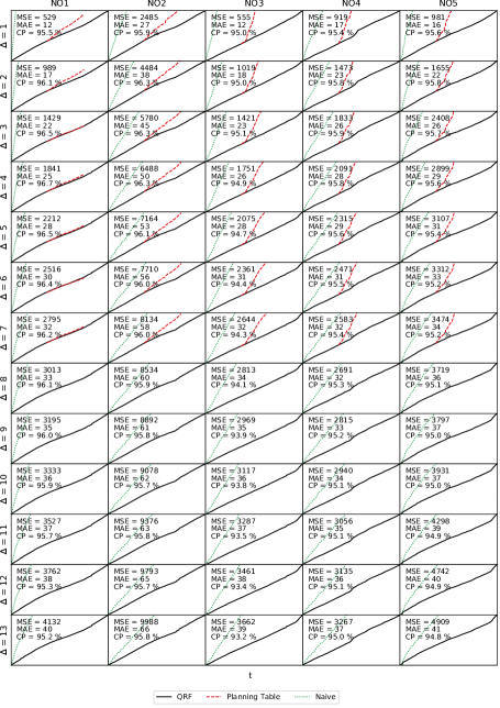
Figure 3 summarizes the results of the described experiments. Each cell plots the cumulative error throughout the year 2016 for the QRF forecasts and benchmarks. Additionally, each cell contains information about the MSE, MAE and CP of the QRF predictions. Each cell stands for a specific prediction target given by market area $\alpha$ and time $t+\Delta$.

Above all, the predicted imbalances are of higher accuracy compared to both benchmarks. As expected, the accuracy of the point predictions declines going further in the future (i.e. with increasing $\Delta$). As desired, the coverage probability is at approximately 95 % across all predictions. Significant is the performance difference for the market areas NO2, NO3, NO4 and NO5, where the QRF predictions are superior compared to the Planning Table.

We use the Scikit Garden implementation of the quantile regression forests.

Prototype

Although the quantitative offline evaluation showed considerable improvements in forecasting imbalances, the actual prototype deployment (and usage by human operators) will demonstrate the usefulness as an accompanying tool next to the Planning Table.

The lower MSE values can be translated to smaller frequency deviations, compared to the Planning Table, if both solution would act as an autonomous system. However, neither of the two are autonomous systems, as already mentioned they act as decision support tools. The human operator has the final decision on the operational measures to take. Hence, after the deployment, we expect to acquire a qualitative feedback from the human operators.

It is worth noting that the research and the deployment of the prototype would not be possible without a tight cooperation with the TSO, i.e. Statnett. Normally, TSOs has conservative and careful approach in introducing new tools in the control room (to the human operators). Nevertheless, the introduced tool cannot (for reasons explained later) and does not aim to replace the Planning Table. Planning Table still remains the main decision support tool, whereas our tool aims to provide more accurate intra-hour imbalance forecasts utilizing historical data.

Discussion

The presented approach has its limitations. Contrary to the Planning Table, the model does not incorporate features such as production plans, consumption forecasts and planned HVDC flows. Thus, it cannot account for rare but foreseen imbalances. This is why the presented approach cannot replace the Planning Table. For future work, it is crucial to take plans and forecasts into account, and learn (reoccurring) patterns.

Additionally, we focus on the problem within the Nordic area. The imbalances may have different character in other electrical power systems, and thus our approach can exhibit better or worse performance, and may require a different feature set.

The presented model does not utilize weather information because those features do not contribute to substantial improvements. We hypothesise that the weather data may provide useful information if the model could incorporate the consumption forecasts, or in electrical power systems with a greater share of intermittent renewable production (e.g. wind and solar power).

Conclusion

In this paper, we proposed a method that applies quantile regression forests to predict two hours ahead imbalances in the form of point predictions and more importantly as prediction intervals. In contrast to known methods reported in the literature, the proposed method relies purely on historical imbalances and features related to date and time, making our method novel for imbalance forecast in general.

An unanticipated finding was that the imbalances exhibit relatively strong and to some extent predictable patterns. Moreover, even though our model operates purely using historical imbalances and temporal features, it was still able to outperform the contemporary solution of the TSO.

Overall, we see this work as an initial step towards a decision support tool, which could in a longer horizon be a fully automated solution that is able to replace the insufficient Planning Table altogether with the human expertise. For future work, we plan to develop a model that incorporates some essential predictors such as consumption forecasts. More importantly, we are in the process of building a prototype system that is able to deliver real-time imbalance forecasts. In addition to being a proof of concept, this prototype system will be deployed in Statnett’s control room and thus provide a complementary tool for the human operators to assess the trend of the upcoming imbalances. Furthermore, we expect to acquire a qualitative feedback from the human operators, which could help us to further improve our method.

References

- [Breiman 2001] Breiman, L. 2001. Random forests. Machine Learning 45:5–32.
- [Contreras 2016] Contreras, C. 2016. System imbalance forecasting and short-term bidding strategy to minimize imbalance costs of transacting in the Spanish electricity market. Master’s thesis, Comillas Pontifical University, ICAI School of Engineering.
- [ENTSO-E 2016] ENTSO-E. 2016. Nordic balancing philosophy. http://bit.ly/2T5uxx0. Accessed 05 September 2018.
- [Garcia and Kirschen 2004] Garcia, M. P., and Kirschen, D. S. 2004. Forecasting system imbalance volumes in competitive electricity markets. IEEE PES Power Systems Conference and Exposition 1115–1122.
- [Glachant and Ruester 2014] Glachant, J.-M., and Ruester, S. 2014. The EU internal electricity market: Done forever? Utilities Policy 31:221 – 228.
- [Håberg and Doorman 2016] Håberg, M., and Doorman, G. 2016. Classification of balancing markets based on different activation philosophies: Proactive and reactive designs. In 2016 13th International Conference on the European Energy Market (EEM), 1–5.
- [Klæboe, Eriksrud, and Fleten 2015] Klæboe, G.; Eriksrud, A. L.; and Fleten, S.-E. 2015. Benchmarking time series based forecasting models for electricity balancing market prices. Energy Systems 6:43–61.
- [Kratochvíl 2016] Kratochvíl, Š. 2016. System Imbalance Forecast. Ph.D. Dissertation, Czech Technical University in Prague, Department of Economics, Management and Humanities.
- [Meinshausen 2006] Meinshausen, N. 2006. Quantile regression forests. Journal of Machine Learning Research 7:983–999.
- [Statnett et al. 2016] Statnett; Fingrid; Energinet.dk; and Svenska Kraftnät. 2016. Challenges and Opportunities for the Nordic power system. http://bit.ly/2DkYPX4. Accessed 20 June 2018.
- [Wangensteen 2012] Wangensteen, I. 2012. Power System Economics: The Nordic Electricity Market. Tapir Academic Press.