Three-Dimensional Supernova Explosion Simulations of 9-, 10-, 11-, 12-, and 13-M_⊙ Stars

Abstract

Using the new state-of-the-art core-collapse supernova (CCSN) code Fornax, we have simulated the three-dimensional dynamical evolution of the cores of 9-, 10-, 11-, 12-, and 13-M_⊙ stars from the onset of collapse. Stars from 8-M_⊙ to 13-M_⊙ constitute roughly 50% of all massive stars, so the explosive potential for this mass range is important to the overall theory of CCSNe. We find that the 9-, 10-, 11-, and 12-M_⊙ models explode in 3D easily, but that the 13-M_⊙ model does not. From these findings, and the fact that slightly more massive progenitors seem to explode (Vartanyan et al., 2019), we suggest that there is a gap in explodability near 12-M_⊙ to 14-M_⊙ for non-rotating progenitor stars. Factors conducive to explosion are turbulence behind the stalled shock, energy transfer due to neutrino-matter absorption and neutrino-matter scattering, many-body corrections to the neutrino-nucleon scattering rate, and the presence of a sharp silicon-oxygen interface in the progenitor. Our 3D exploding models frequently have a dipolar structure, with the two asymmetrical exploding lobes separated by a pinched waist where matter temporarily continues to accrete. This process maintains the driving neutrino luminosty, while partially shunting matter out of the way of the expanding lobes, thereby modestly facilitating explosion. The morphology of all 3D explosions is characterized by multiple bubble structures with a range of low-order harmonic modes. Though much remains to be done in CCSN theory, these and other results in the literature suggest that, at least for these lower-mass progenitors, supernova theory is converging on a credible solution.

1 Introduction

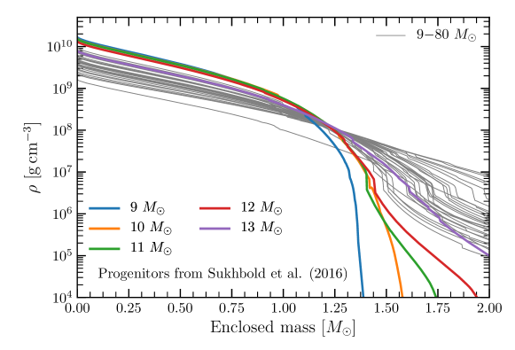
Approximately $\sim$50% of the mass function of massive stars above $\sim$8.0 M_⊙ lies below $\sim$13.0 M_⊙. Since only stars more massive than $\sim$8.0 M_⊙ can end their lives as core-collapse supernovae (CCSNe) (simultaneously giving birth to either neutron stars or black holes), understanding the mechanism and character of supernova explosions (if they occur) in this modest mass range, assumes an outsized astrophysical importance. Traditionally, those who model the core-collapse and explosion phases of massive stars inherit progenitor models at the cusp of core collapse from experts in massive star evolution. The latter simulate a star’s passage through successive burning phases until an unstable Chandrasekhar white dwarf core emerges at the star’s center, at which point the physical profiles of that core are mapped onto the grid of a supernova code to carry the dynamical, oftimes multi-dimensional, evolution forward. Aside from the stochasticity and chaos associated with the turbulence that attends both progenitor and supernova convective instabilities, the structure of the roughly spherical “initial" model determines the outcome of the supernova simulation, and, it is hoped, the outcome of stellar death. In particular, a progenitor’s radial mass density profile seems to determine much of the subsequent explosive behavior. Figure 1 portrays a representative collection of such profiles. It has been observed, indeed with quantitative variations from modeler to modeler and with some degree of non-monotonic behavior with progenitor ZAMS mass (Woosley & Heger, 2007; Sukhbold et al., 2016; Sukhbold et al., 2018), that massive stars at the lower end of the mass function have steeper mass density profiles with radius than those at the higher end.

It is thought that such steep profiles result in cores that explode easily by the proto-neutron star (PNS) neutrino-driven wind mechanism (Burrows, 1987; Burrows et al., 1995), even in one-dimension (1D, spherical), and this has been shown to be the case (Kitaura et al., 2006; Fischer et al., 2010; Radice et al., 2017) for the pioneering 8.8-M_⊙ model of Nomoto (Nomoto, 1984, 1987). However, such “electron-capture" supernovae (ECSNe) occupy a problematic region of model space (Woosley & Heger, 2015), one in which burning under electron-degenerate conditions with subsequent flashes could 1) eject envelope matter before collapse, 2) radically restructure the core, or 3) compromise the accuracy of 1D stellar evolution simulations. Nevertheless, spherical progenitor models with masses from 8.1 M_⊙ to 9.6 M_⊙, and steep density profiles in the outer Chandrasekhar mantle, have exploded in 1D CCSN simulations (Kitaura et al., 2006; Fischer et al., 2010; Müller et al., 2012; Melson et al., 2015a; Radice et al., 2017). These supernova models universally involve low explosion energies ($\sim$10⁵⁰ ergs $\equiv$ 0.1 Bethe). When performed in 2D (Burrows et al., 2007; Müller et al., 2012; Radice et al., 2017) or 3D (for the 9.6 M_⊙ model; Melson et al. (2015a)), the explosions are not only low-energy, but quasi-spherical, and such explosions are likely to yield low-mass neutron stars with low-velocity neutron star kicks. A reasonable conclusion is that if the progenitor mass density profiles are as steep as found in these models (Figure 1), the theory and rough explosion numbers arrived at using modern supernova codes that incorporate neutrino transport and heating may be roughly reproducing Nature.

However, the 1D and 2D supernova models of Radice et al. (2017) for the 9, 10, 11 M_⊙ progenitor models of Sukhbold et al. (2016), though spanning a low-mass segment of progenitor parameter space and manifesting a monotonic sequence in mass-density profile from very steep to progressively less steep, do not behave monotonically, nor do they all explode easily. The 9-M_⊙ model explodes easily in 2D by a neutrino-driven wind mechanism (though not in 1D), but the 10-M_⊙ model does not explode in 1D or 2D without significant progenitor velocity perturbations (Couch & Ott, 2013; Müller & Janka, 2015; Müller et al., 2017; Abdikamalov et al., 2016; Takahashi et al., 2016). On the other hand, as with the 9-M_⊙ model, the 11-M_⊙ model does not explode in 1D, but does explode in 2D, and without the aid of perturbations. Moreover, the 12-M_⊙ model of Woosley & Heger (2007), simulated in 2D by Burrows et al. (2018), Vartanyan et al. (2018) and O´Connor & Couch (2018b), does not explode at all unless aided by such things as rotation or significant velocity perturbations (Vartanyan et al., 2018), but the 16-M_⊙ progenitor model from Woosley & Heger (2007) with a significantly shallower mass density profile explodes easily in 2D and 3D (Vartanyan et al., 2019). Collectively, this behavior with variations in mass density profile along the progenitor mass continuum, for which in this mass range the “compactness" parameter (O’Connor & Ott, 2011, 2013; Ott et al., 2018) is monotonic demonstrates once again that the compactness parameter is not predictive of “explodability" (Burrows et al., 2018).

Supernova modeling experience in the recent past now suggests that as the progenitor mass density profile shallows explodability by the wind mechanism is at first easy, and then difficult or impossible. However, with still shallower profiles, explosions by a convection-aided, neutrino-driven mechanism become easier again, though this is not a classic wind. For these progenitors, the post-bounce, pre-explosion mass accretion rates are large enough to result in larger mass densities between the stalled shock wave and PNS core. The correspondingly larger neutrino absorption optical depths in this mantle region lead to more efficient neutrino heating that, with the aid of multi-dimensional effects (Herant et al., 1994; Burrows et al., 1995; Murphy & Burrows, 2008), ignites an explosion. These massive stars have the potential to yield larger explosion energies, with larger kick speeds and neutron star masses. Such explosions are also aided by the accretion of steep silicon/oxygen interfaces (Vartanyan et al., 2018). The associated discontinuity in the mass accretion rate through the shock results in a decrease in the inhibiting tamp, but there is a delay in the corresponding decrease in the neutrino luminosity due to the finite advection time between the shock and the inner core. By accompanying a temporarily unaltered neutrino luminosity with an immediate decrease in the ram pressure, the shock wave can be kicked into explosion by suddenly achieving the critical condition (Burrows & Goshy, 1993). For progenitors with initial mass density profiles intermediate between those of these exploding classes, post-bounce accretion smothers the wind, while failing to provide a large enough neutrino optical depth in the mantle. To date, for these progenitor structures, currently residing near $\sim$12 M_⊙ (Woosley & Heger, 2007; Sukhbold et al., 2016; Sukhbold et al., 2018), 1D and 2D supernova models do not explode in the context of the default physics employed, carried out for as long as one second post-bounce, and without initial rotation nor substantial progenitor seed perturbations. However, we reiterate that the progenitor profiles for massive stars have not theoretically converged and, moreover, that the mapping between ZAMS mass and progenitor structure has not been definitively settled (Woosley & Heger, 2007; Sukhbold et al., 2016; Sukhbold et al., 2018; Meakin et al., 2011; Couch et al., 2015; Müller et al., 2016, 2017).

In this paper, using our new supernova code Fornax (see §2 and Skinner et al. (2019), we simulate in three spatial dimensions (3D) the self-consistent behavior at the lower-mass end (9-, 10-, 11-, 12-, and 13-M_⊙) of a suite of supernova progenitors from Sukhbold et al. (2016). This work is in part a 3D extension of our earlier 1D and 2D study (Radice et al., 2017). As stated earlier, these masses span a large fraction of the mass function.

An earlier generation of pioneering 3D simulations (Hanke et al., 2013; Tamborra et al., 2014; Couch & O’Connor, 2014; Melson et al., 2015a; Melson et al., 2015b; Lentz et al., 2015; Müller, 2015; Takiwaki et al., 2016; Roberts et al., 2016; Ott et al., 2018; O’Connor & Couch, 2018a; Summa et al., 2018; Glas et al., 2018a), employing various necessary simplifications, have set the stage for this study, but 3D simulations are still rare. Moreover, some earlier work did not include inelastic scattering nor velocity-dependent transport (Couch & O’Connor, 2014; Ott et al., 2018; Roberts et al., 2016), did not include inelastic scattering on nucleons (Glas et al., 2018a), employed “ray-by-ray+" dimensional reduction (Hanke et al., 2013; Tamborra et al., 2014; Lentz et al., 2015; Müller, 2015; Melson et al., 2015a; Melson et al., 2015b; Takiwaki et al., 2016; Summa et al., 2018), cut out the inner core, or performed the simulations in the inner core in 1D. Depending upon how large this inner 1D core was, the latter procedure could suppress, partially or in full, PNS convection (Dessart et al., 2006; Radice et al., 2017; Glas et al., 2018b). Such convection has been shown to facilitate the explosion of some models (Radice et al., 2017).

Though still expensive, our 3D Fornax runs avoid all these issues, and are state-of-the-art, but still compromise on aspects of the problem. In particular, we employ the two-moment closure M1 method (Vaytet et al., 2011; Skinner et al., 2019), which is not multi-angle. In addition, our energy-group number and spatial resolution should be increased, perhaps significantly, to ensure the results are converged. Furthermore, we use approximate general relativity (GR) to address the enhanced attractive strength of GR and gravitational redshifts, and not full GR (Roberts et al., 2016; Ott et al., 2018). Finally, we lump the $\nu_{\mu}$, $\bar{\nu}_{\mu}$, $\nu_{\tau}$, and $\bar{\nu}_{\tau}$ neutrinos into one species. It has been suggested that this approach can have its limitations (Bollig et al., 2017). Nevertheless, Fornax belongs to a new generation of CCSN simulation codes now emerging with 3D radiation/hydrodynamic capabilities that, though resource-intensive and perforce incorporating various and sundry approximations, finally promise to address the core-collapse supernova phenomenon with full physical fidelity.

In §2, we briefly summarize our computational setup and the microphysics incorporated into Fornax. Then, in §3 we present the central results and derived quantities of our 3D simulations. Following this, in §4 we discuss the characteristics of the explosion debris field and morphology, and then in §5 we recap our most important findings, summarize the current status of supernova theory, and speculate on productive future directions.

2 Methods and Setup

All the 3D and 2D runs performed in this paper used the multi-group radiation/hydrodynamics code Fornax. To date, results using this new capability have been published in Skinner et al. (2016), Wallace et al. (2016), Radice et al. (2017), Vartanyan et al. (2018), Burrows et al. (2018), Skinner et al. (2019), and Vartanyan et al. (2019). The methodologies and equations solved are described in detail in Skinner et al. (2019). The full suite of microphysics and the approach to approximate general relativity (GR) employed are summarized in Vartanyan et al. (2019), in particular in Appendices A and B, respectively, in that paper. We restrict the calculation of gravity to the monopole term, corrected for approximate GR (Marek et al., 2006) and including gravitational redshifts of the neutrino spectra. The comoving-frame transport is a multi-dimensional variant of the two-moment scheme M1 (Vaytet et al., 2011), with analytic closures for the second and third radiation moments (Skinner et al., 2019). Weak magnetism and recoil effects are handled using the formulae in Horowitz (2002) without truncation. Velocity-dependent transport terms to order $(v/c)$ are included, inelastic energy redistribution for neutrino-electron and neutrino-nucleon scattering are handled using the method of Thompson et al. (2003) and Burrows & Thompson (2004), and detailed neutrino-matter scattering and absorption opacities are calculated using the formulations of Burrows et al. (2006), augmented to include the many-body correction to the neutrino-nucleon scattering rates of Horowitz et al. (2017). The latter progressively decreases these neutral-current scattering opacities with increasing density in a manner that approximately captures the associated many-body physics (Burrows & Sawyer, 1998). The effects of this term on core-collapse physics and phenomenology are explored in Burrows et al. (2018) and Vartanyan et al. (2018).

We simulated the multi-D transport of the electron-type neutrinos ($\nu_{e}$), anti-electron-type neutrinos ($\bar{\nu}_{e}$), and “$\nu_{\mu}$"s, where the latter bundles the $\nu_{\mu}$, $\bar{\nu}_{\mu}$, $\nu_{\tau}$, and $\bar{\nu}_{\tau}$ neutrinos. In 3D, we used twelve energy groups for each species, spanning 1 to 300 MeV for the $\nu_{e}$s and 1 to 100 MeV for the others and in 2D we used twenty energy groups over the same ranges.

The calculations were all performed using the same spherical, dendritic grid (Skinner et al., 2019), which deresolves the angular zoning as the center is approached to roughly maintain the same aspect ratio of the spatial zones in the inner $\sim$20 kilometers and to minimize the Courant penalty of spherical convergence. The zoning was 678$\times$128$\times$256 ($r\times\theta\times\phi$) in 3D and 678$\times$256 ($r\times\theta$) in 2D. The inner zone had a $\Delta{r}$ of 0.5 kilometers, and the radial zoning was roughly constant in the inner $\sim$20 km and logarithmic exterior to $\sim$20 kilometers out to an outer spatial boundary of 20,000 kilometers. The 3D runs were begun 10 milliseconds after bounce and were mapped from a corresponding 1D run and continued forward in 3D.

Though 9, 10, and 11 M_⊙ simulations in Radice et al. (2017) employed the non-rotating progenitors from Sukhbold et al. (2016), as we do here for all our models (see Figure 1), the EOS used in that study was that of Lattimer & Swesty (1991) (LS220). Because the SFHo (Steiner et al., 2013) EOS is still consistent with all known nuclear and astrophysical constraints (Tews et al., 2017), whereas the LS220 EOS no longer is, we have opted to use the SFHo EOS in this study. Therefore, we have redone for this paper the comparison 2D simulations for the 9, 10, and 11 M_⊙ progenitors using the SFHo EOS. Also, whereas Radice et al. (2017) investigated the effects of the many-body corrections of Horowitz et al. (2017) (see also Burrows et al. (2018) and Burrows & Sawyer (1998)) to the neutral-current scattering rates off free nucleons, we here include such corrections by default.

A number of authors have touted the potential role of perturbations due to pre-supernova turbulence (Couch & Ott, 2013; Müller & Janka, 2015; Müller et al., 2017; Abdikamalov et al., 2016; Takahashi et al., 2016), preliminary 3D progenitor models are now emerging (Couch et al., 2015; Müller et al., 2017), and Radice et al. (2017) and Vartanyan et al. (2018) have compared various models with and without perturbations. For our 3D runs, we imposed slight $\ell=10$/$m=1$/$n=4$ velocity perturbations on the initial 3D model between 200 and 1000 kilometers, using the scheme of Müller & Janka (2015), as implemented by Radice et al. (2017). However, the magnitude of these perturbations, meant to seed instabilities that might arise, was only 100 km s^-1. This is to be compared with the radial speed of tens of thousands of km s^-1 at the beginning of the 3D phase. This prescription imposes a minimal degree of perturbation merely to seed turbulence and seems irrelevant to the viability of the explosions we witness. We impose the same perturbations for the comparison 2D simulations, evaluating them in this case at $\phi=0$. Hence, it is highly unlikely that these perturbations played any substantive role in the subsequent growth of turbulence, and were likely dwarfed in effect by the “grid noise."

This paper is meant in part to be a three-dimensional continuation of the 2D and 1D study in Radice et al. (2017). However, that paper explored 9, 10, 11, 8.1, 8.8, and 9.6 M_⊙ models, while we here focus on the 9, 10, 11, 12, and 13 M_⊙ models of Sukhbold et al. (2016). Since the 8.1 and 9.6 M_⊙ progenitors investigated by Radice et al. (2017) were for $10^{-4}$ and zero metallicity and our goals here are to understand the common core-collapse supernova phenomenon, we drop these models from further consideration. In addition, since there is no model in Sukhbold et al. (2016) that corresponds to the 8.8 M_⊙ progenitor of Nomoto (Nomoto, 1984) or that is lower in mass than 9.0 M_⊙, the latter mass serves as the lower mass limit of this study.

3 Basic Explosion Results

Tables 1 and 2 provide some useful summary numbers associated with our 3D and 2D core-collapse simulations. For Table 1, the explosion energy, the baryon and gravitational masses of the residual proto-neutron star, the average PNS radius (defined as the average radius interior to an isodensity surface at 10¹¹ g cm^-3), and the envelope binding energy of the off-grid material exterior to 20,000 kilometers (km) are given at t(final), the time post-bounce at the end of each simulation. All the models, except the 13-M_⊙ model, explode. Table 2 lists the mean shock radii and speeds at the end of each simulation. In 3D, the former range from $\sim$15,200 km to $\sim$2,600 km. Since all the exploding models have diagnostic energies (see below) at the end of the calculation in excess of the off-grid overburden energy (see Table 1), these numbers should continue to increase.

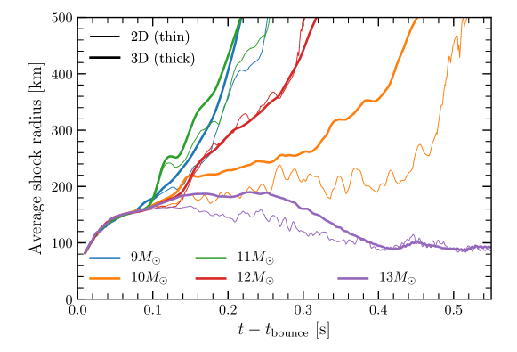
Figure 2 depicts the first 0.55 seconds after bounce of the evolution of the mean shock radius for both 3D (thick) and 2D (thin) models. Except for the 13-M_⊙ model, all the 3D and 2D models explode. As indicated on this figure, all the models evolve similarly in the first $\sim$100 milliseconds. This is a consequence of the characteristic timescale in this study for convection and turbulence to kick in and reflects the very small initial seed perturbations imposed (see §2). It is in part the breaking of symmetry due to the onset of turbulence, with its associated dynamics and turbulent stresses, that enables the divergence of the behaviors of the various stalled shocks. The mean shock radii of the 9-M_⊙ and 11-M_⊙ models never really stall or recede and these models explode within $\sim$100 milliseconds of bounce. As with many of our models, the 9-M_⊙ core explodes immediately upon accretion through the partially stalled shock of its sharp silicon/oxygen interface (Vartanyan et al., 2018). The core of the 12-M_⊙ progenitor requires $\sim$40 milliseconds longer to launch its explosion, while the 10-M_⊙ model takes rather much longer to supernova, but is clearly doing so by $\sim$0.3 and $\sim$0.45 seconds in 3D and 2D, respectively. Generally, the 3D models explode slightly earlier than the 2D models, though for the 12-M_⊙ progenitor the 3D and 2D models are launched at roughly the same time. This behavior is consonant with that found by Vartanyan et al. (2019) for the 16-M_⊙ star from Woosley & Heger (2007), who observed that for this progenitor the 3D explosion preceded the 2D explosion by $\sim$50 milliseconds. We note that using their FMD (fully-multi-dimensional) code AENUS-ALCAR, which did not incorporate redistribution by inelastic scattering nor the many-body correction to neutral-current neutrino-nucleon scattering (Horowitz et al., 2017), Glas et al. (2018a) also found that their 3D model exploded before their 2D model, though it exploded at $\sim$300 ms after bounce, later than we find. This difference could easily reflect differences in numerical approach and microphysics. Why the 3D models explode earlier than the 2D models is unclear, but was anticipated in Dolence et al. (2013).

As stated earlier, the 13-M_⊙ model in this progenitor suite does not explode in either 2D or 3D. As Figure 1 demonstrates, this model not only has a shallower density profile (and, therefore higher post-bounce mass accretion rates), but a more muted density jump at its silicon/oxygen interface relative to that of the other “low-mass" progenitors highlighted in this paper. This interface also resides further out in interior mass. These factors clearly have a bearing on the outcome we find. Due to its steep density profile, the 9-M_⊙ model transitions rather quickly to a neutrino-driven wind explosion (Burrows, 1987) and achieves a low asymptotic explosion energy near 0.1 Bethe. The 10-M_⊙, 11-M_⊙, and 12-M_⊙ models explode similarly weakly (though quickly), due in part to the low absorbing mass (hence, low neutrino optical depth) in the gain region (Bethe & Wilson, 1985) and the low driving $\nu_{e}$ and $\bar{\nu}_{e}$ neutrino luminosities. Both the low luminosities (which are powered in this early phase mostly by accretion) and low neutrino optical depths are consequences of the steep core mass density profiles of these 9-M_⊙, 10-M_⊙, 11-M_⊙, and 12-M_⊙ models. However, it seems that for these models the positive effect of post-shock turbulence and neutrino heating outweigh the negative effects of the accretion ram and the critical condition for explosion (Burrows & Goshy, 1993; Murphy & Burrows, 2008) can be met. But as the mass density shallows and if the Si/O interface is more subtle, we witness a decreasing tendency to explode, as manifest by our result for the 13-M_⊙ progenitor. However, as our positive result for the corresponding 16-M_⊙ progenitor (Vartanyan et al., 2019) demonstrates, explodability returns despite a shallower, higher density mantle. For such models the neutrino optical depth and accretion-powered luminosities are more significant and, particularly if the Si/O interface jump is not small, “explodability" seems to return. Therefore, we are seeing a gap in explodability, near 13-M_⊙ for the Sukhbold et al. (2016) progenitor models and our Fornax implementation (§2). We saw a similar gap at 12-M_⊙ in Burrows et al. (2018) and Vartanyan et al. (2018) for the 2D models of those studies with a different progenitor suite (Woosley & Heger, 2007), as did O´Connor & Couch (2018b). Hence, it may well be that 1) the lowest-mass progenitors experience low-energy (one to a few$\times$10⁵⁰ ergs?) explosions that are partially wind-like; 2) higher-mass progenitors experience higher-energy explosions due to higher driving luminosities and neutrino absorption optical depths in the gain region, despite the higher accretion ram tamp; and 3) there is a gap in explodability. It may be that some flavor of rotation, or new/better physics and numerics, could close this gap, but currently the presence of a gap in explodability, as indicated by our 3D calculations to date, seems plausible. We emphasize that the “compactness parameter" (O’Connor & Ott, 2011) of the 9-M_⊙ through our 16-M_⊙ (Vartanyan et al., 2019) models we have studied to date is monotonic with progenitor mass, but that the outcomes are not.

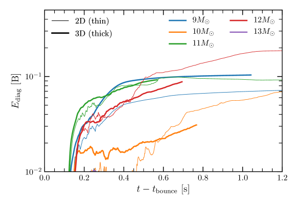
Figure 3 portrays the “diagnostic" explosion energy (Melson et al., 2015a) evolution for our 9-, 10-, 11-, and 12-M_⊙ 3D and 2D models. Since the 13-M_⊙ model does not explode in either 3D or 2D, it does not appear as one of the plotted lines. By diagnostic energy, we mean the sum of the gravitational, kinetic, thermal, and recombination energies of the ejecta. The ejecta are defined as matter that instantaneously appears unbound by the standard Bernoulli condition, and the diagnostic energy does not include the binding energy of the matter exterior to our 20,000-kilometer outer boundary. The latter is given in Table 1 and we see that in all exploding cases the diagnostic energy has overcome the mantle binding term by the end of all our simulations, and is still climbing for most. In fact, the total asymptotic explosion energy (Table 1) is indeed positive for all our exploding models, though those energies are still modest and seem destined to be no more than $\sim$one to a few$\times$10⁵⁰ ergs. However, for this low-mass massive star subset, this may be realistic (Morozova et al., 2018). The 9-M_⊙ models have total explosion energies (in 3D and 2D) that have almost asymptoted. We note that our 3D 9-M_⊙ model is one of the only state-of-the-art 3D models in the literature to have approached an asymptotic value.

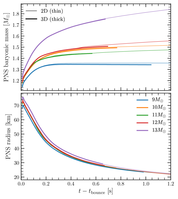
Figure 4 provides the evolution of both the baryon mass (top) and PNS radius (bottom) for both the 3D (thick) and 2D (thin) models. The final values of the residue’s baryon mass (those achieved by the end of each simulation), along with the corresponding gravitational masses, are given in Table 1. We see that the neutron star left behind in the 3D 9-M_⊙ explosion has a baryonic mass of 1.342 M_⊙ and a gravitational mass of 1.246 M_⊙. These values are on the low end of the observed pulsar mass distribution and reflect the lower accretion rates and early explosion times of this model. As suggested in Table 1, such low masses seem to be generic for the steeper density profiles that obtain in this low-mass supernova progenitor mass range. Since the 13-M_⊙ models don’t explode and the associated progenitor density profile is the shallowest of the set (implying higher mass accretion rates), the corresponding 3D and 2D PNS baryon masses are large (1.714 [3D] and 1.854 [2D] M_⊙ at simulation end) and are still growing fast at the termination of the runs.

Müller (2015) observes in his long-term study of the 11.2 M_⊙ model of Woosley et al. (2002) that the explosion energy accumulates more unsteadily in 2D than in 3D. In Figure 3 in the early explosion stages, we too see that the 2D explosion energies accumulate more unsteadily than in 3D, but at later times accumulate smoothly. Moreover, we observe for all our models that the residual PNS masses are similar in 2D and 3D. This is in contradistinction to what was found in Müller (2015) and reflects the similar accretion histories in 2D and 3D we witness; what differences there are seem correlated mostly with the (slight) differences in explosion times. An important difference with the Müller (2015) investigation, other than the different code, EOS, and transport methods employed in each study, is that we include as a default in our microphysics suite the Horowitz et al. (2017) many-body correction to the neutrino-nucleon scattering rates. As noted, this facilitates explosion and may mitigate some of the accretional differences between 2D and 3D highlighted in Müller (2015). However, a full exploration of the phenomena called out in Müller (2015) awaits a more exhaustive study that includes longer-term simulations of a broader set of stellar progenitor masses.

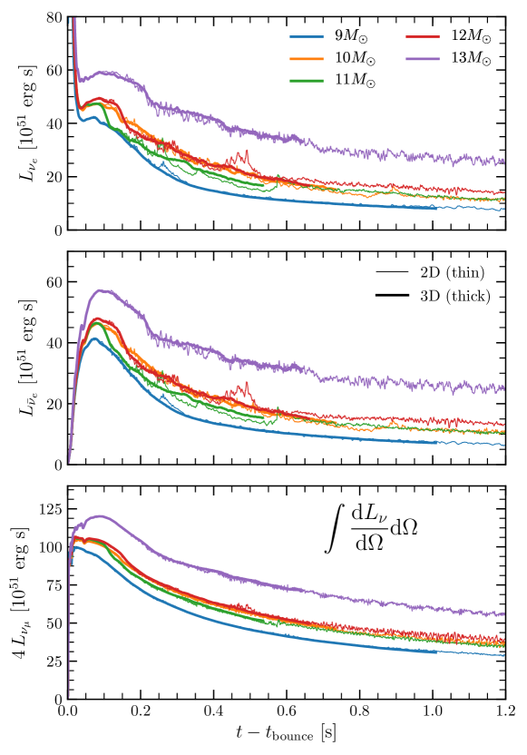
The PNS radii are defined as the average radius at a density of 10¹¹ g cm^-3. As determined in Radice et al. (2017), due to enhanced outward transport and the alteration of inner entropy and Y_e profiles, PNS convection increases this radius beyond what would obtain in 1D. The similarity of the 3D and 2D curves in Figure 4 reflects the similar luminosity and core energy loss rates from the interior in 3D and 2D. This fact is reinforced by Figure 5, which demonstrates that the luminosity evolutions in 2D and 3D are nearly the same. We note in passing that the solid-angle-integrated luminosities in 3D evolve more smoothly in time than in 2D, wherein axial sloshing and hydrodynamic asymmetries are more pronounced.

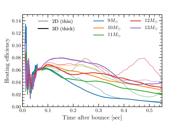
Figure 6 depicts the neutrino heating efficiency, defined as the ratio of the heating rate due to $\nu_{e}$ and $\bar{\nu}_{e}$ absorption in the gain region and the sum of the $\nu_{e}$ and $\bar{\nu}_{e}$ luminosities. This quantity does not include the heating due to inelastic scattering off electrons and nucleons, though this effect is included in the calculations and amounts to a sub-dominant $\sim$5-15% of the total. We see in Figure 6 that the efficiency ranges from a few to $\sim$8% and is similar in 3D and 2D prior to explosion. For the non-exploding 13-M_⊙ model, the 3D and 2D curves do not much differ during the entire simulation, but for the exploding models, since the explosion times differ in 3D and 2D (generally being later in 2D), the associated curves depart from one another after the first of the models explodes. We note that higher efficiencies do not translate into a greater tendency to explode, as witnessed by the behavior of the 13-M_⊙ model. We also note that the neutrino-driven mechanism is not a “1% phenomenon," as frequently considered, but in this context is closer to a “5$-$6%" phenomenon.

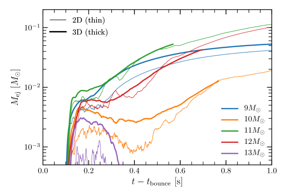
Figure 7 shows the evolution of the ejecta mass (in units of M_⊙) versus time after bounce (in seconds, up to a maximum of one second) for both the 3D (thick) and 2D (thin) models. Only the “qualifying" matter on our computational grid interior to the 20,000-kilometer radius of the initial progenitor models is included in this quantity, but it is likely that all the matter exterior to the 20,000-kilometer outer boundary for the exploding models will in fact be ejected. Some matter for the 13-M_⊙ models that did not eventually explode still achieved for a short time the Bernoulli condition we have used to identify the ejecta. At the end of the simulations, the ejecta mass (as defined here) for the exploding models ranges from $\sim$10^-2 to $\sim$10^-1 M_⊙.

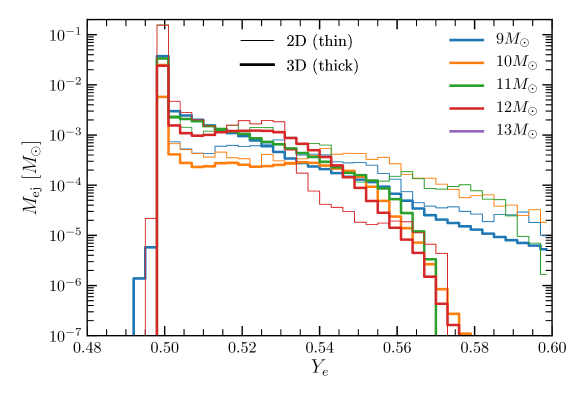
Figure 8 renders histograms of the final Y_e distributions for the 3D (thick) and 2D (thin) models calculated. This is a true histogram for which the total ejecta mass in a particular Y_e bin is the mass given on the y-axis. Importantly, M_ej on the ordinate is not a distribution function in Y_e (i.e., not $\frac{dM}{dY_{e}}$) and the actual sum of the histogram values given here is the last total ejecta mass plotted in Figure 7 and/or given at the final time listed in Table 1. We find that the total ejecta mass with Y_e = 0.5 for the 3D models ranges between $\sim$5$\times$ and $\sim$40$\times$10^-2 M_⊙ and provides a scale for the ⁵⁶Ni mass ejected. However, we did not perform nucleosynthetic calculations for these runs and are leaving such studies to an upcoming new generation of 3D calculations. As Figure 8 shows, the ejecta for the 3D and 2D runs are not vastly different and are generally proton rich, extending up beyond Y_e = 0.56, with most of the ejecta near 0.5. The ejecta Y_es are a consequence of the competition between $\nu_{e}$ and $\bar{\nu}_{e}$ absorption and, hence, quite dependent on the fidelity with which the neutrino-matter coupling is handled. This fact should be borne in mind and puts a premium on accurate neutrino transport.

4 Explosion Morphologies

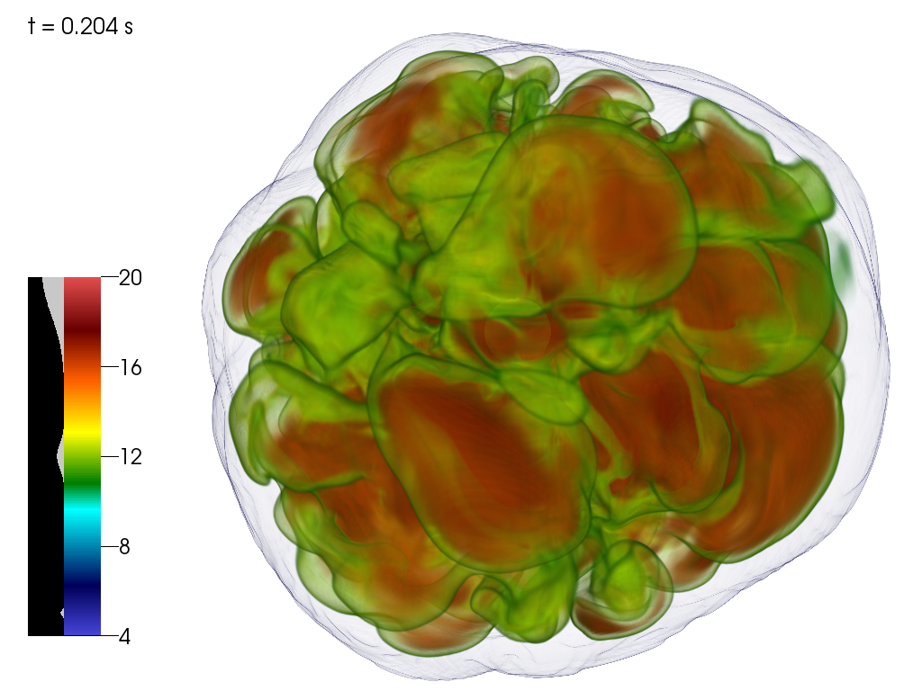
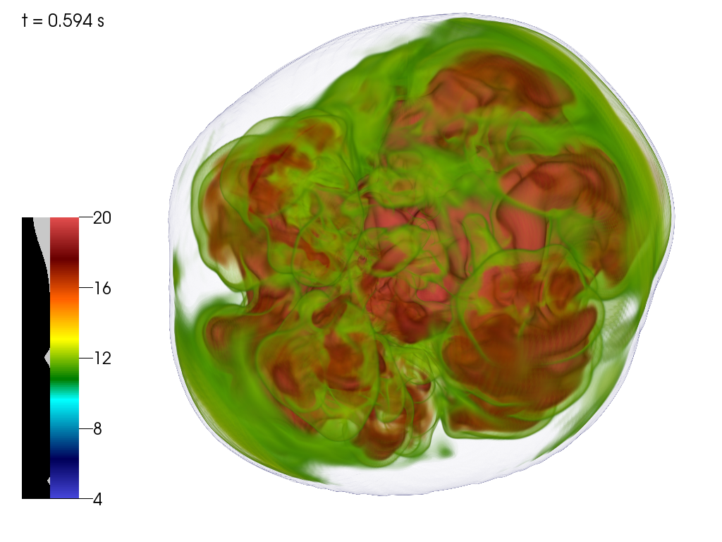
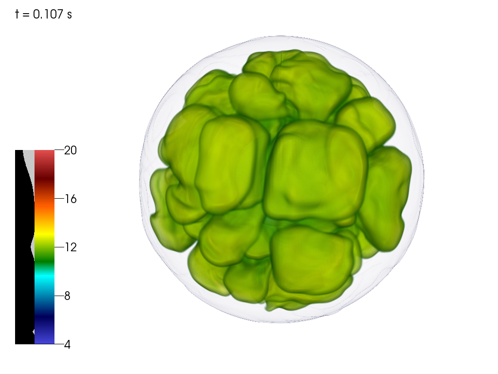
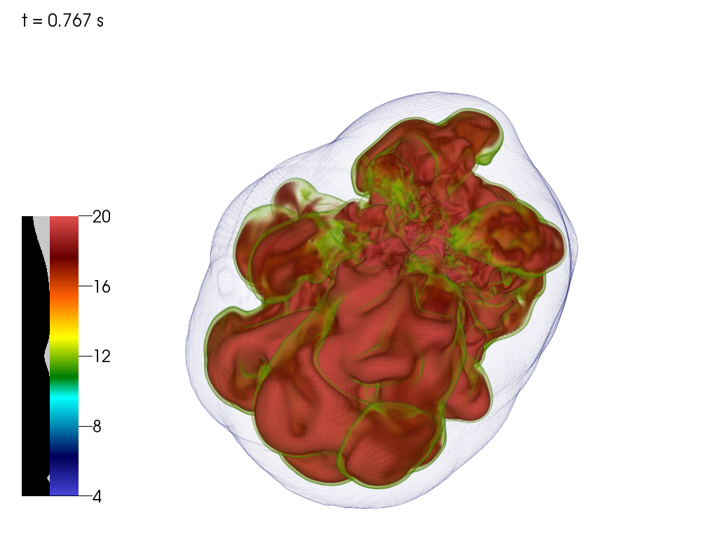
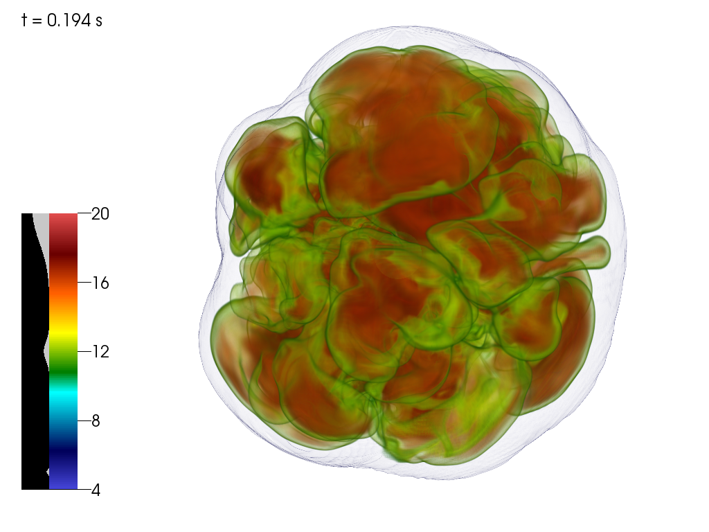
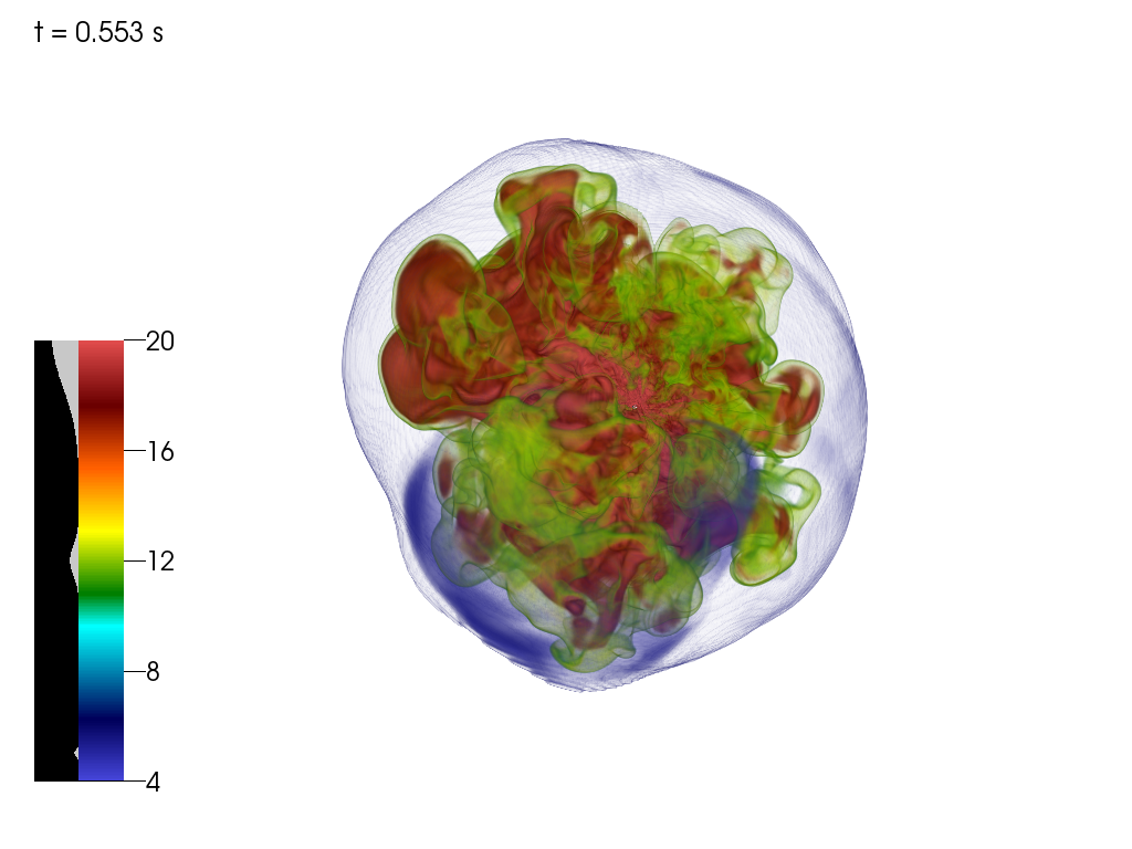
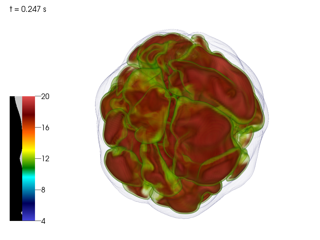
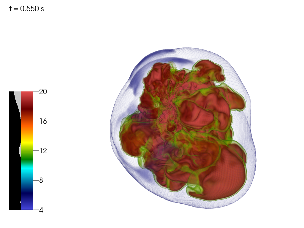
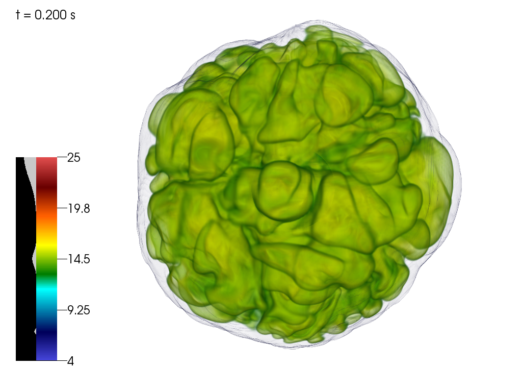
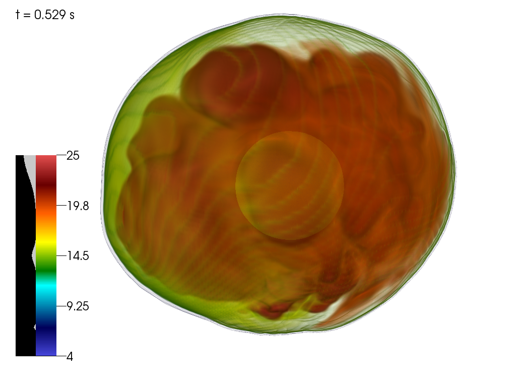
Figures 9 through 12 depict snapshots of volume renderings of the entropy distributions for the 9-M_⊙, 10-M_⊙, 11-M_⊙, and 12-M_⊙ models interior to the shock wave. This post-shock mantle material 1) first participates in the turbulent convection exterior to the PNS core and interior to the stalled shock prior to explosion (left slide) and then 2) constitutes, along with the outer matter encompassed by the expanding shock, the neutrino-driven bubbles and mushroom clouds of the subsequent explosion (right slide). The outer blue shroud is the shock wave. Recall that the 13-M_⊙ model (Figure 13) does not explode and that both its shock wave and PNS core eventually shrink as the core deleptonizes and cools.

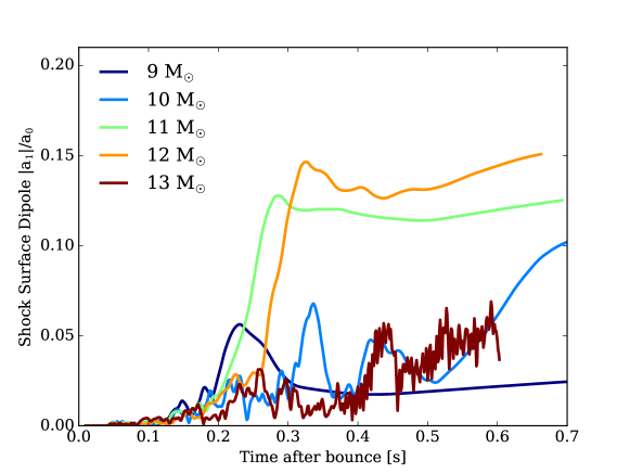
Prior to explosion, the characteristic physical scale of the neutrino-driven turbules behind the shock is set by the size of the gain region. This is tens of kilometers to $\sim$100 kilometers and generally represents less than or equal to 50% of the shock radius (to the center). Hence, the angle subtended by the turbules is tens of degrees, which translates into modes of $\ell$ = 5$-$10. To be sure, this is a crude estimate, but serves as a useful mnemonic. However, as the explosion commences, the dominant harmonic components of the shock position itself are predominantly the monopole (clearly) and the dipole. In fact, most exploding models have a growing dipole (Dolence et al., 2013), whose growth seems in phase with that of the monopole (whose growth itself constitutes a zeroth-order marker of explosion). For these non-rotating models, the direction chosen by the dipole (a vector) seems arbitrary and is not correlated with the coordinate axes (fortunately), but is correlated with the kick direction (Radice et al. 2019, in preparation). This emphasizes the conclusion that the explosions of such stochastic and chaotic models without physically defined directions would in reality span a uniform spectrum of directions. Figure 14 depicts the monopole-normalized dipole magnitude versus time after bounce for the five 3D models of this paper. The harmonic decomposition employed to generate this figure is that found in Burrows et al. (2012) and Vartanyan et al. (2019). The explosions of our 11-M_⊙ and 12-M_⊙ models are particularly asymmetrical and dipolar, with the dipole component of the shock surface of the 10-M_⊙ model growing fast at the end of that simulation, while by that metric the 3D 9-M_⊙ model is much more spherical. That the latter is more spherical makes sense, since this model explodes almost immediately and a dipole mode doesn’t seem to have time to grow.

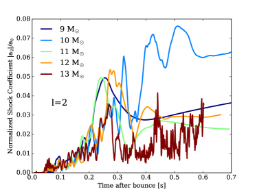
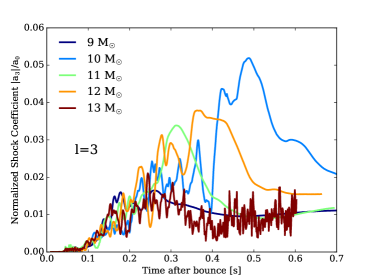
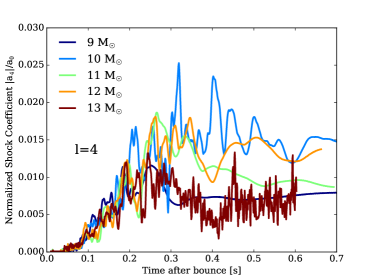
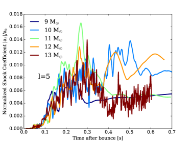
Figure 15 renders the corresponding evolution for the normalized higher-order spherical harmonics ($\ell=2,3,4,5$) of the deformation of the shock surface in 3D. For the 3D model results in both Figures 14 and 15, we have lumped together in quadrature the azimuthal $m$s in an effort to avoid the significant clutter that would attend their separate inclusion. However, there is much information in this more refined azimuthal decomposition and we will explore in the future ways to represent it.

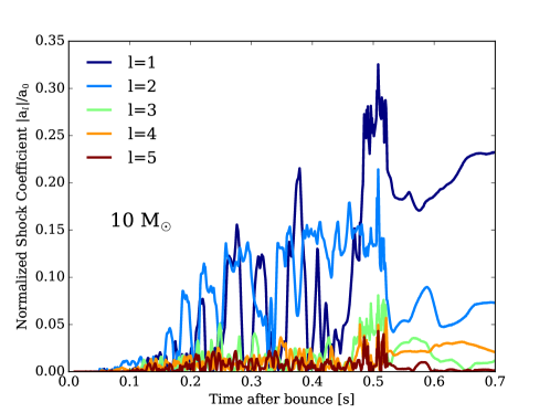
We observe that for a given progenitor model the magnitude of the higher-order harmonic coefficients generally decreases as $\ell$ increases and that for the non-exploding 13-M_⊙ model all $\ell$s below six remain of rather low relative amplitude. As both Figures 14 and 15 demonstrate, all the non-monopolar components start small and grow with time as turbulent convection builds. The speed with which this occurs reflects in part the character and magnitude of the seed perturbations, which for all our models are quite small. After explosion onset, for all models the higher-order normalized $\ell$ coefficients grow and then saturate, or grow, peak, slightly diminish, and then saturate (or assume a more secular, long-term drift), with the dipole and quadrupole terms usually predominating in relative magnitude. The time at which the normalized amplitudes of the various harmonics peaks correlates with the explosion time, with the coefficients for the 9-M_⊙ model evolving most quickly through its stages. For this most spherical of our 3D models, the amplitudes of the higher-harmonics remain rather small. For the more-delayed 10-M_⊙ model, the dipole term remains small until explosion is fully underway, and then strengthens (as it does for those models that explode earlier). Before this phase, its normalized shock quadrupole is roughly comparable to its corresponding dipole. Curiously, only the dipole component is of real significance for the 11-M_⊙ model; all its other modes peak early and then assume rather small values. For all models, the temporal fluctuations of all components are significant before explosion, but damp out after explosion as the ejecta evolve into a more coasting, nearly homologous, phase. For the non-exploding 13-M_⊙ model, fluctuations remain rapid on the roughly $\sim$10-millisecond timescales of the turbulence in the gain region. For comparison, we portray in Figure 16 the evolution of the normalized $\ell=1,2,3,4,5$ shock harmonics for the 10-M_⊙ model in 2D. This choice of progenitor is meant merely to be representative. We notice immediately the larger amplitude of the temporal fluctuations in 2D until the simulation is well into explosion, the clear hierarchy in harmonic order with $\ell$, and the larger asymptotic values of the dipole and quadrupole coefficients in 2D than in 3D. The latter are clearly artifacts of the 2D constraint.

We emphasize that all explosions are dominated interior to the shock by bubble structures in mass and entropy, not surprisingly very much like mushroom clouds, with higher harmonic order and angular scales of $\sim$30$-$60 degrees. At late times, but before instabilities in the outer reaches of the massive star can come into play (Utrobin et al., 2018), the bubble structures freeze into a quasi-homologous expansion with frozen angular scales, reflecting the approximate freezing of the associated shock surface structure. However, we note that the influence of computational resolution on the morphology and angular scales of the debris has yet to be determined.

As seen in our 3D 16-M_⊙ explosion model (Vartanyan et al., 2019), two lobes sometimes characterize the debris field, with a “wasp-like" waist separating the two exploding lobes of different sizes (see also Müller (2015), his Figure 6). We see something like this for the 10-M_⊙ and 12-M_⊙ 3D models, but not for the 9-M_⊙ and 11-M_⊙ 3D models and it is curious (perhaps coincidental?) that those former models explode the latest. For a time during the early explosion, this waist, when it appears, is the region where matter is still accreting onto the PNS core in an annular region. This continued accretion helps maintain the driving $\nu_{e}$ and $\bar{\nu}_{e}$ neutrino luminosities, which is emitted more isotropically, despite the directed character of wasp-waist accretion. Such annular accretion seems to funnel matter away from the exploding lobes, thereby diminishing the tamp they experience and, perhaps, facilitating explosion. In some sense, this partial funnelling of matter from antipodal regions into which matter is exploding to an annular region that, at early times, is not exploding is akin to a quadrupolar ($\ell=2$) symmetry breaking in the velocity field and may be a mode found by the outer flow to encourage explosion. Numerous questions emerge, among which are: 1) Is it the case that some models employ such a quadrupolar instability to facilitate explosion? and 2) Given a progenitor, how predictable is the character of the debris field and what is the distribution of explosion morphologies for a given star? We don’t yet know the answers to these questions, but these are worthy future lines of investigation.

The debris fields and morphologies that we have described and that are represented in Figures 9 through 12 are but the initial conditions for the ⁵⁶Ni-bubble, Rayleigh-Taylor, and Richtmyer-Meshkov instability phases and reverse shocks experienced by the ejecta (Fryxell et al., 1991; Kifonidis et al., 2003; Utrobin et al., 2018) at later times as the blast traverses the outer star. We also note that, aside from the 9-M_⊙ model, our exploding 3D models have not yet asymptoted to their final energies and PNS configurations, though they have achieved positive total explosion energies. Finally, for the non-exploding 13-M_⊙ model, there is some indication at late times of the development of a spiral “SASI" mode (Blondin & Shaw, 2007; Blondin & Mezzacappa, 2007; Rantsiou et al., 2011) and whether this will transition into an explosion at very late times (Takiwaki et al., 2016), though unlikely, has yet to be determined. Other than this late-time manifestation in our 3D 13-M_⊙ run, we don’t witness the classical SASI (Blondin et al., 2003) in any of our simulations. This is in keeping with the conclusion by Burrows et al. (2012) that the SASI is more likely to be in evidence for non-exploding models and that in exploding models neutrino-driven convection generally overwhelms it. However, the final word on the appearance and importance of the SASI has yet to be written.

5 Conclusions

Our new 3D results, and those 1D, 2D, and 3D results of others (Kitaura et al., 2006; Burrows et al., 2007; Fischer et al., 2010; Müller et al., 2012; Melson et al., 2015a; Radice et al., 2017) for this lower-mass range, now suggest that these stars can easily explode by the delayed neutrino mechanism with explosion energies not far from what is observationally expected (Morozova et al., 2018). Moreover, with the results articulated here and elsewhere in the recent literature (e.g., Burrows et al. (2018); Vartanyan et al. (2019)), we can conclude that various features and/or processes disproportionately support or determine explosion in the context of the neutrino heating paradigm. These include 1) turbulence behind the stalled shock wave; 2) the progenitor density structure, in particular the magnitude of the discontinuity at the silicon/oxygen interface; 3) neutrino heating by inelastic neutrino-electron and neutrino-nucleon scattering; 4) many-body corrections to neutrino-nucleon scattering rates (Burrows et al., 2018; Horowitz et al., 2017); and 5) the magnitude and distribution of seed perturbations (Couch & Ott, 2013, 2015; Müller et al., 2017) (though not explored here). We have found in this paper that most low-mass progenitor models explode in 3D, but that there may be a mass gap for the current generation of progenitor models near 12$-$14 M_⊙ where explosion is a bit more problematic. This does not mean that these stars don’t explode, merely that there is a hint from our simulation experience using state-of-the-art tools and modern stellar progenitors that non-rotating cores in this intermediate mass range are less explodable. In addition, we see in our 3D simulations, as with the previous generation of 2D simulations, that simultaneous explosion and accretion (in different solid-angle sectors at a given time) helps maintain explosion in its early phases in some directions by continuing to power the emergent luminosity with an accretion component in other directions. This can’t happen in 1D, but with such a broken symmetry in multi-D it can. Related to this is a wasp-waist pinched structure seen in some debris distributions and the strong dipolar character to many ejecta fields. Moreover, and again (Burrows et al., 2018), we see that compactness parameter in and of itself is not predictive of explosion.

Though the 3D calculations in this new tranche of full-physics supernova models suggest that we and the community of supernova theorists have reached an important milestone in the theory of core-collapse supernovae with the routine generation of sophisticated 3D explosion simulations, there are a number of caveats that bear listing. First, though not outdone by any extant full-physics 3D runs, the spatial and energy-group resolution of our simulations should be improved $-$ a resolution study is in order. Second, we have implemented and fielded with Fornax an approximate GR variant, wherein the correction to the monopolar strength of gravity has been addressed, along with the gravitational redshift of the neutrinos, but bonafide GR (Kuroda et al., 2016; Ott et al., 2018) has been left to later development. Third, we have employed a many-body correction to the axial-vector coupling term in the neutrino-nucleon scattering rates that is still approximate (Horowitz et al., 2017) and have not incorporated the still-uncalculated corresponding correction to the charged-current absorption rates (Burrows & Sawyer, 1999; Roberts et al., 2012; Roberts & Reddy, 2017). Since we have here and elsewhere (Burrows et al., 2018; Vartanyan et al., 2018) found such effects to be important, this remains an important topic for future investigation. Fourth, for this study we have employed the SFHo EOS and though competitive it is not definitive. The dependence of the outcome of stellar collapse on the EOS remains to be determined in full. Fifth, though we perform truly 3D neutrino transfer solving for two angular moments of the specific intensity with a vector neutrino flux, this is not multi-angle transport. The assumed tensor closure form is an ansatz and the higher-order moments (second and third) are provided analytically (Vaytet et al., 2011). Though for pseudo-spherical problems such an approach can be quite accurate (Richers et al., 2017), ultimately full Boltzmann transport in seven dimensions (three space, three momentum space, and time), currently too expensive, will be necessary. In addition, it may well be that aspects of neutrino oscillations must be factored in, raising yet further the ultimate necessary level of computational complexity. Sixth, the mapping between progenitor structure and ZAMS mass is still in flux. Though palpable and enduring progress has been made these last few decades in determining the character of massive star evolution, since the density, seed perturbation, and rotational profiles of the collapsing cores of massive stars are not yet reliably determined in detail, one should be cautious in declaring what a given mass star might do at the end of its life. In addition, we note that core rotation can affect the outcomes, but that rapid rotation that results in neutron-star spin periods less $\sim$50 milliseconds should be rare (Faucher-Giguère & Kaspi, 2006). Such a rotation period is considered “slow" by CCSN theorists. Nevertheless, there is such a densely-packed range in published massive-star structures for the full range of ZAMS masses (see Figure 1) that we find it difficult to conclude that what is now in the literature does not span a realistic range of progenitor structures. However, and importantly, chaos and stochasticity in the turbulent pre-supernova phases will translate into a spread of outcomes in all the astronomical observables (e.g., explosion energies, kick velocities, final neutron star spins and masses, nucleosynthesis, debris spatial distributions). What these spreads are is currently unknown.

Hence, there still remains much to do in CCSN theory that will keep investigators busy for many years. Nevertheless, with the recent emergence of sophisticated codes such as Fornax to generate multiple 3D simulations every year, we have entered a new era in the study of supernova explosions. No longer is the community limited to one or a few expensive 3D runs per year whose individual import is ambiguous. Now, with adequate computational resources many, many full-physics 3D simulations per year are possible. This enables the broader exploration of parameter space and can lead to a more forgiving theoretical environment. The few inevitable mistakes necessary to make real progress in a science are no longer as dire. The last two decades marked the era of commodity 2D simulations that facilitated real progress in parameter exploration and constituted a palpable leap in overall understanding. After $\sim$50 years of development in physics, technique, and computational capabilities, we have now entered the corresponding era in 3D modeling. As a result, with good reason can we expect in the years to come, further (and final?) leaps in insight into this, one of the last remaining fundamental theoretical challenges of stellar astrophysics.

Figure 1: The mass-density ($\rho$, in g cm^-3) versus interior mass (in units of M_⊙) for various representative progenitor models from Sukhbold et al. (2016). The profiles for the 9-, 10-, 11-, 12-, and 13-M_⊙ models are highlighted in color. Comparisons between these and the other profiles (in gray) up to 80-M_⊙ put this lower-mass subclass into the larger context of progenitor initial models. Note that the 13-M_⊙ model is distinct from the others highlighted in this low-mass progenitor study. See the text for a discussion.

Figure 2: The solid-angle-weighted average shock wave radius (in kilometers) versus time after bounce (in seconds) for the 9-, 10-, 11-, 12-, and 13-M_⊙ models of this study in 3D (thick) and 2D (thin). All the 3D and 2D models, except the 13-M_⊙ model, explode. Shown are the radii until 0.55 seconds after bounce, though the runs were frequently carried out further (see Table 1). The 9-M_⊙ and 11-M_⊙ models explode within $\sim$100 milliseconds of bounce, the 12-M_⊙ progenitor requires $\sim$40 milliseconds longer, while the 10-M_⊙ model is clearly exploding by $\sim$0.3 and 0.45 seconds in 3D and 2D, respectively. Generally, the 3D models explode slightly earlier than the 2D models, though for the 12-M_⊙ progenitor the 3D and 2D models are launched at roughly the same time. We note that the 13-M_⊙ model in this progenitor model suite not only does not explode in either 2D or 3D, but that it has a muted silicon/oxygen interface jump in density (and entropy) relative to that of the others (see Figure 1) that resides further out in interior mass. These factors seem to have an impact on the “explodability" of that core. Moreover, in Burrows et al. (2018) and Vartanyan et al. (2018), the 2D 12-M_⊙ model, using default physics, did not explode, but this initial model was from a different progenitor suite (Woosley & Heger, 2007) for which the 12-M_⊙ model does not have as pronounced a silicon/oxygen density discontinuity. See the text for a discussion of these trends.

Figure 3: Diagnostic explosion energies (in Bethes, $\equiv$ 10⁵¹ ergs) versus time after bounce (in seconds) for the 9-, 10-, 11-, and 12-M_⊙ models calculated for this investigation. Note that since the 13-M_⊙ model does not explode in either 3D or 2D it does not register as one of the plotted lines (it would have been purple). The thick lines are for the 3D models and the thin lines are for the 2D models. The diagnostic energy includes the sum of the gravitational, kinetic, thermal, and recombination energies of the ejecta, but not the binding energy of the off-grid matter exterior to our 20,000-kilometer outer boundary. However, as can be seen in Table 1, the outer envelope binding energies for each of these low-mass models are quite small. We note that the 9-M_⊙ models have total explosion energies (in 3D and 2D) that have almost asymptoted to their final values. See text for a discussion.

Figure 4: The corresponding proto-neutron star baryon masses (in units of M_⊙) and radii (in units of kilometers) versus time after bounce (in seconds). The radii are defined as the average at a density of 10¹¹ g cm^-3. The 3D models are the thick lines, while the 2D models are the thin lines. Note that the residual baryon masses for the 9-M_⊙ models have asymptoted, those for the other models are still growing (slightly), and those for the 13-M_⊙ model (which don’t explode) are still growing quickly. The final gravitational masses (Table 1) for the exploding models range comfortably from 1.23 M_⊙ to 1.36 M_⊙.

Figure 5: The evolution with time after bounce (in seconds) of the neutrino luminosities (in units of 10⁵¹ erg s^-1) for the 3D (thick) and 2D (thin) model sets. Shown from top to bottom are the curves for the $\nu_{e}$, $\bar{\nu}_{e}$, and “$\nu_{\mu}$" species. Note that the 3D and 2D luminosity curves are solid-angle-averaged and are quite similar. This reflects similar core deleptonization and cooling rates and similar mass accretion histories (in 3D and 2D) for the quasi-spherical cores and is expected.

Figure 6: The neutrino heating efficiency versus time after bounce (in seconds) for all the 3D and 2D models simulated in this paper. The efficiency is defined as the ratio of the neutrino heating rate due to $\nu_{e}$ and $\bar{\nu}_{e}$ absorption on nucleons in the gain region and the sum of the $\nu_{e}$ and $\bar{\nu}_{e}$ luminosities. The efficiency ranges from a few to $\sim$8% and is similar in 3D and 2D prior to explosion, but differs after explosion. See text for a discussion.

Figure 7: The ejecta mass (in units of M_⊙), defined as the mass on positive Bernoulli trajectories, versus time after bounce (in seconds, up to a maximum of one second) for both the 3D (thick) and 2D (thin) models. Here, we are tagging only matter on our computational grid interior to the 20,000-kilometer radius of the initial progenitor models. For the exploding models, it is likely that all the matter exterior to the 20,000-kilometer outer boundary will in fact be ejected, but this has yet to be definitively determined. Note that some matter for the 13-M_⊙ models that did not eventually explode still achieved for a short time the Bernoulli condition we have used to tag the ejecta. At the end of the simulations, the ejecta mass (as defined here) for the exploding models ranges from $\sim$10^-2 to $\sim$10^-1 M_⊙.

Figure 8: Histograms of the final (end of simulation, see Table 1) Y_e distributions for the 3D (thick) and 2D (thin) models calculated. This is a true histogram for which the total ejecta mass in a particular Y_e bin is the mass given on the ordinate (y-axis). M_ej on the ordinate is not a distribution function in Y_e (i.e., not $\frac{dM}{dY_{e}}$). We note that the total ejecta mass with Y_e = 0.5 for the 3D models ranges between $\sim$5$\times$ and $\sim$40$\times$10^-2 M_⊙ and provides a scale for the ⁵⁶Ni mass ejected. However, we also note that we did not perform true nucleosynthetic calculations for these runs and are leaving such studies to an upcoming new generation of 3D calculations.

Figure 9: Two representative stills during the post-bounce 3D evolution of the exploding 9-M_⊙ model. Time proceeds from left to right and the spatial scale expands as a function of time. The outer blue shroud is the shock wave. The representation is a volume rendering of the entropy at the post-bounce time given in each top-left corner (in seconds) and the associated color map given in the bottom-left corner. The entropy units are per baryon per Boltzmann’s constant. High entropies in the shocked mantle are more conducive to explosion, but entropy alone does not determine a predilection towards explosion. The physical scales (approximate diameter of the shock) are 400 km (left) and 6000 km (right). Note that, as with the following figures, the last time depicted here is not the last time of the simulation (see Table 1). See the text for a discussion of this and related plots.

Figure 10: Same as Figure 9, but for the 10-M_⊙ model. Note that the entropy scales are the same as in Figure 9, but that snapshot times are different. The physical scales (approximate diameter of the shock) are 200 km (left) and 2700 km (right).

Figure 11: Same as Figure 9, but for the 11-M_⊙ model. Note that the entropy scales are the same as in Figure 9, but that snapshot times are different. The physical scales (approximate diameter of the shock) are 420 km (left) and 4000 km (right).

Figure 12: Same as Figure 9, but for the 12-M_⊙ model. Note that the entropy scales are the same as in Figure 9, but that snapshot times are different. The physical scales (approximate diameter of the shock) are 436 km (left) and 2500 km (right).

Figure 13: Same as Figure 9, but for the 13-M_⊙ model. Note that the entropy scales are the same as in Figure 9, but that snapshot times are different. By that the end of the simulation this model had not exploded and the shock radius had shrunk significantly. The circles dimly seen in the centers of the two rightmost figures trace the PNS "surface," defined as the surface where $\rho=10^{11}$ g cm^-3. As indicated in Table 2, at the last time depicted here the PNS radius was $\sim$30 kilometers. The physical scales (approximate diameter of the shock) are 200 km (left) and 100 km (right).

Figure 14: The amplitude of the dipole component of the shock surface, normalized by the corresponding monopole term, as a function of the time after bounce (in seconds). The algorithm for calculating this quantity is taken from Burrows et al. (2012). The five 3D models of this plot are indicated by different colors. Note that the ramp up of the dipolar component (when it occurs) roughly coincides with the onset of explosion (Table 1). See the text for a discussion.

Figure 15: Similar to Figure 14, but for the $\ell=2,3,4,5$ harmonic coefficients of the shock surface (normalized to the monopole term) versus time since bounce (in seconds). $\ell=2$ is in the top left, $\ell=3$ is in the top right, $\ell=4$ is in the bottom left, and $\ell=5$ is in the bottom right. As in Burrows et al. (2012), for the 3D models and the various $\ell$s the $m$ subcomponent terms are added in quadrature. See the text for a discussion.

Figure 16: Similar to the panels in Figure 15, but for the $\ell=1,2,3,4,5$ harmonic coefficients of the shock surface (normalized to the monopole term) of the 2D 10-M_⊙ model. See the text for a discussion.

References

- Abdikamalov et al. (2016) Abdikamalov E., Zhaksylykov A., Radice D., Berdibek S., 2016, MNRAS, 461, 3864
- Bethe & Wilson (1985) Bethe H. A., Wilson J. R., 1985, ApJ, 295, 14
- Blondin & Mezzacappa (2007) Blondin J. M., Mezzacappa A., 2007, Nature, 445, 58
- Blondin & Shaw (2007) Blondin J. M., Shaw S., 2007, ApJ, 656, 366
- Blondin et al. (2003) Blondin J. M., Mezzacappa A., DeMarino C., 2003, ApJ, 584, 971
- Bollig et al. (2017) Bollig R., Janka H.-T., Lohs A., Martínez-Pinedo G., Horowitz C. J., Melson T., 2017, Physical Review Letters, 119, 242702
- Burrows (1987) Burrows A., 1987, ApJ, 318, L57
- Burrows & Goshy (1993) Burrows A., Goshy J., 1993, ApJ, 416, L75
- Burrows & Sawyer (1998) Burrows A., Sawyer R. F., 1998, Phys. Rev. C, 58, 554
- Burrows & Sawyer (1999) Burrows A., Sawyer R. F., 1999, Phys. Rev. C, 59, 510
- Burrows & Thompson (2004) Burrows A., Thompson T. A., 2004, in Fryer C. L., ed., Astrophysics and Space Science Library Vol. 302, Astrophysics and Space Science Library. pp 133–174, doi:10.1007/978-0-306-48599-2_5
- Burrows et al. (1995) Burrows A., Hayes J., Fryxell B. A., 1995, ApJ, 450, 830
- Burrows et al. (2006) Burrows A., Reddy S., Thompson T. A., 2006, Nuclear Physics A, 777, 356
- Burrows et al. (2007) Burrows A., Dessart L., Livne E., 2007, in Immler S., Weiler K., McCray R., eds, American Institute of Physics Conference Series Vol. 937, Supernova 1987A: 20 Years After: Supernovae and Gamma-Ray Bursters. pp 370–380, doi:10.1063/1.3682931
- Burrows et al. (2012) Burrows A., Dolence J. C., Murphy J. W., 2012, ApJ, 759, 5
- Burrows et al. (2018) Burrows A., Vartanyan D., Dolence J. C., Skinner M. A., Radice D., 2018, Space Sci. Rev., 214, 33
- Couch & O’Connor (2014) Couch S. M., O’Connor E. P., 2014, ApJ, 785, 123
- Couch & Ott (2013) Couch S. M., Ott C. D., 2013, ApJ, 778, L7
- Couch & Ott (2015) Couch S. M., Ott C. D., 2015, ApJ, 799, 5
- Couch et al. (2015) Couch S. M., Chatzopoulos E., Arnett W. D., Timmes F. X., 2015, ApJ, 808, L21
- Dessart et al. (2006) Dessart L., Burrows A., Livne E., Ott C. D., 2006, ApJ, 645, 534
- Dolence et al. (2013) Dolence J. C., Burrows A., Murphy J. W., Nordhaus J., 2013, ApJ, 765, 110
- Faucher-Giguère & Kaspi (2006) Faucher-Giguère C.-A., Kaspi V. M., 2006, ApJ, 643, 332
- Fischer et al. (2010) Fischer T., Whitehouse S. C., Mezzacappa A., Thielemann F.-K., Liebendörfer M., 2010, A&A, 517, A80
- Fryxell et al. (1991) Fryxell B., Mueller E., Arnett D., 1991, ApJ, 367, 619
- Glas et al. (2018b) Glas R., Janka H.-T., Melson T., Stockinger G., Just O., 2018b, arXiv e-prints,
- Glas et al. (2018a) Glas R., Just O., Janka H.-T., Obergaulinger M., 2018a, preprint, (arXiv:1809.10146)
- Hanke et al. (2012) Hanke F., Marek A., Müller B., Janka H.-T., 2012, ApJ, 755, 138
- Hanke et al. (2013) Hanke F., Müller B., Wongwathanarat A., Marek A., Janka H.-T., 2013, ApJ, 770, 66
- Herant et al. (1994) Herant M., Benz W., Hix W. R., Fryer C. L., Colgate S. A., 1994, ApJ, 435, 339
- Horowitz (2002) Horowitz C. J., 2002, Phys. Rev. D, 65, 043001
- Horowitz et al. (2017) Horowitz C. J., Caballero O. L., Lin Z., O’Connor E., Schwenk A., 2017, Phys. Rev. C, 95, 025801
- Kifonidis et al. (2003) Kifonidis K., Plewa T., Janka H.-T., Müller E., 2003, A&A, 408, 621
- Kitaura et al. (2006) Kitaura F. S., Janka H.-T., Hillebrandt W., 2006, A&A, 450, 345
- Kuroda et al. (2016) Kuroda T., Takiwaki T., Kotake K., 2016, ApJS, 222, 20
- Lattimer & Swesty (1991) Lattimer J. M., Swesty F. D., 1991, Nuclear Physics A, 535, 331
- Lentz et al. (2015) Lentz E. J., et al., 2015, ApJ, 807, L31
- Marek et al. (2006) Marek A., Dimmelmeier H., Janka H.-T., Müller E., Buras R., 2006, A&A, 445, 273
- Meakin et al. (2011) Meakin C. A., Sukhbold T., Arnett W. D., 2011, Ap&SS, 336, 123
- Melson et al. (2015a) Melson T., Janka H.-T., Marek A., 2015a, ApJ, 801, L24
- Melson et al. (2015b) Melson T., Janka H.-T., Bollig R., Hanke F., Marek A., Müller B., 2015b, ApJ, 808, L42
- Morozova et al. (2018) Morozova V., Piro A. L., Valenti S., 2018, ApJ, 858, 15
- Müller (2015) Müller B., 2015, MNRAS, 453, 287
- Müller & Janka (2015) Müller B., Janka H.-T., 2015, MNRAS, 448, 2141
- Müller et al. (2012) Müller B., Janka H.-T., Heger A., 2012, ApJ, 761, 72
- Müller et al. (2016) Müller B., Viallet M., Heger A., Janka H.-T., 2016, ApJ, 833, 124
- Müller et al. (2017) Müller B., Melson T., Heger A., Janka H.-T., 2017, MNRAS, 472, 491
- Murphy & Burrows (2008) Murphy J. W., Burrows A., 2008, ApJ, 688, 1159
- Nomoto (1984) Nomoto K., 1984, ApJ, 277, 791
- Nomoto (1987) Nomoto K., 1987, ApJ, 322, 206
- O’Connor & Couch (2018a) O’Connor E., Couch S., 2018a, preprint, (arXiv:1807.07579)
- O´Connor & Couch (2018b) O´Connor E. P., Couch S. M., 2018b, ApJ, 854, 63
- O’Connor & Ott (2011) O’Connor E., Ott C. D., 2011, ApJ, 730, 70
- O’Connor & Ott (2013) O’Connor E., Ott C. D., 2013, ApJ, 762, 126
- Ott et al. (2018) Ott C. D., Roberts L. F., da Silva Schneider A., Fedrow J. M., Haas R., Schnetter E., 2018, ApJ, 855, L3
- Radice et al. (2017) Radice D., Burrows A., Vartanyan D., Skinner M. A., Dolence J. C., 2017, ApJ, 850, 43
- Rantsiou et al. (2011) Rantsiou E., Burrows A., Nordhaus J., Almgren A., 2011, ApJ, 732, 57
- Richers et al. (2017) Richers S., Nagakura H., Ott C. D., Dolence J., Sumiyoshi K., Yamada S., 2017, ApJ, 847, 133
- Roberts & Reddy (2017) Roberts L. F., Reddy S., 2017, Phys. Rev. C, 95, 045807
- Roberts et al. (2012) Roberts L. F., Reddy S., Shen G., 2012, Phys. Rev. C, 86, 065803
- Roberts et al. (2016) Roberts L. F., Ott C. D., Haas R., O’Connor E. P., Diener P., Schnetter E., 2016, ApJ, 831, 98
- Skinner et al. (2016) Skinner M. A., Burrows A., Dolence J. C., 2016, ApJ, 831, 81
- Skinner et al. (2019) Skinner M. A., Dolence J. C., Burrows A., Radice D., Vartanyan D., 2019, ApJS, 241, 7
- Steiner et al. (2013) Steiner A. W., Hempel M., Fischer T., 2013, ApJ, 774, 17
- Sukhbold et al. (2016) Sukhbold T., Ertl T., Woosley S. E., Brown J. M., Janka H.-T., 2016, ApJ, 821, 38
- Sukhbold et al. (2018) Sukhbold T., Woosley S. E., Heger A., 2018, ApJ, 860, 93
- Summa et al. (2018) Summa A., Janka H.-T., Melson T., Marek A., 2018, ApJ, 852, 28
- Takahashi et al. (2016) Takahashi K., Iwakami W., Yamamoto Y., Yamada S., 2016, ApJ, 831, 75
- Takiwaki et al. (2016) Takiwaki T., Kotake K., Suwa Y., 2016, MNRAS, 461, L112
- Tamborra et al. (2014) Tamborra I., Raffelt G., Hanke F., Janka H.-T., Müller B., 2014, Phys. Rev. D, 90, 045032
- Tews et al. (2017) Tews I., Lattimer J. M., Ohnishi A., Kolomeitsev E. E., 2017, ApJ, 848, 105
- Thompson et al. (2003) Thompson T. A., Burrows A., Pinto P. A., 2003, ApJ, 592, 434
- Utrobin et al. (2018) Utrobin V., Wongwathanarat A., Janka H.-T., Mueller E., Ertl T., Woosley S., 2018, arXiv e-prints,
- Vartanyan et al. (2018) Vartanyan D., Burrows A., Radice D., Skinner M. A., Dolence J., 2018, MNRAS, 477, 3091
- Vartanyan et al. (2019) Vartanyan D., Burrows A., Radice D., Skinner M. A., Dolence J., 2019, MNRAS, 482, 351
- Vaytet et al. (2011) Vaytet N. M. H., Audit E., Dubroca B., Delahaye F., 2011, J. Quant. Spectrosc. Radiative Transfer, 112, 1323
- Wallace et al. (2016) Wallace J., Burrows A., Dolence J. C., 2016, ApJ, 817, 182
- Woosley & Heger (2007) Woosley S. E., Heger A., 2007, Phys. Rep., 442, 269
- Woosley & Heger (2015) Woosley S. E., Heger A., 2015, ApJ, 810, 34
- Woosley et al. (2002) Woosley S. E., Heger A., Weaver T. A., 2002, Reviews of Modern Physics, 74, 1015