Spectral content of a single non-Brownian trajectory

Abstract

Time-dependent processes are often analysed using the power spectral density (PSD), calculated by taking an appropriate Fourier transform of individual trajectories and finding the associated ensemble-average. Frequently, the available experimental data sets are too small for such ensemble averages, and hence it is of a great conceptual and practical importance to understand to which extent relevant information can be gained from $S(f,T)$, the PSD of a single trajectory. Here we focus on the behavior of this random, realization-dependent variable, parametrized by frequency $f$ and observation-time $T$, for a broad family of anomalous diffusions—fractional Brownian motion (fBm) with Hurst-index $H$—and derive exactly its probability density function. We show that $S(f,T)$ is proportional—up to a random numerical factor whose universal distribution we determine—to the ensemble-averaged PSD. For subdiffusion ($H<1/2$) we find that $S(f,T)\sim A/f^{2H+1}$ with random-amplitude $A$. In sharp contrast, for superdiffusion $(H>1/2)$ $S(f,T)\sim BT^{2H-1}/f^{2}$ with random amplitude $B$. Remarkably, for $H>1/2$ the PSD exhibits the same frequency-dependence as Brownian motion, a deceptive property that may lead to false conclusions when interpreting experimental data. Notably, for $H>1/2$ the PSD is ageing and is dependent on $T$. Our predictions for both sub- and superdiffusion are confirmed by experiments in live cells and in agarose hydrogels, and by extensive simulations.

I Introduction

The power spectral density of any time-dependent process $X_{t}$ is a fundamental feature of its spectral content, dynamical behavior and temporal correlations norton . It is an important measure for various processes across many disciplines, including loudness of musical recording voss ; geisel , evolution of climate data talkner , time gaps between large earthquakes sornette , retention times of chemical tracers in groundwater kirchner , noise in graphene devices balandin , fluorescence intermittency in nanosystems fran , current fluctuations in nanoscale electrodes krapf , stochastic processes with random reset satya , some extremal properties of Brownian motion krapivsky , diffusion in strongly disordered systems enzo ; dean , and ionic currents across nanopores ramin1 , to name a few diverse examples.

In its standard definition, the power spectral density (PSD) is the Fourier transform of the autocorrelation function of $X_{t}$ over an infinitely large observation time $T$, i.e., it is an ensemble-averaged property taken in the limit $T\to\infty$. In many situations, however, one cannot create a sufficiently large statistical sample to achieve a reliable ensemble average, and even though the limit $T\to\infty$ can be formally taken in mathematical expressions, it cannot be reached in experiments. Instead, one often deals with either a single or a few individual finite-length realizations of the process, particularly, in experimental data dealing with in vivo systems noerregaard , climate change climatechange , or financial markets eco . In this regard, a question of immense conceptual and practical importance is whether one can learn relevant information about the system from the PSD of just a single or a few finite-length realizations.

Several recent studies examined the PSD from such single-trajectory data. Power spectra of individual time-series were examined for a stochastic model describing blinking quantum dots nie ; QD and also for single-particle tracking experiments with tracers in artificially crowded fluids mat . Notably, the scaling exponent of the power spectrum computed from a few single-trajectory PSDs remains very stable. In addition, the power spectra of the velocity of motile amoeba revealed a robust large-$f$ asymptotic behavior of the form $1/f^{2}$, for all measured individual trajectories li ; ped .

Without a solid mathematical theory, these observations nie ; QD ; mat ; li ; ped may be considered merely as curious coincidences. However, in a recent work diego (see also the perspective ulrich ), it was proven that for standard Brownian motion, the single-trajectory PSD $S(f,T)$ in the large-$f$ limit and at finite $T$ exhibits the same $f$-dependence as its traditional ensemble-average counterpart. This mathematical prediction was fully corroborated by numerical simulations and experiments with polystyrene beads in aqueous solution diego .

Despite its ubiquitous appearance in nature frey , Brownian motion is just a particular example of a stochastic process, and there is no evidence that the same behavior should hold for other naturally occurring transport processes. In this regard, it seems highly desirable to have an analogous proof for anomalous diffusion, with mean-squared displacement (MSD)

$$\langle X_{t}^{2}\rangle\sim t^{\alpha},$$ (1)

and anomalous diffusion exponent $\alpha\neq 1$, where the brackets here and henceforth denote the average over the statistical ensemble.

Such processes are widely observed in soft matter, condensed matter and biological systems, e.g., diffusion in viscoelastic and crowded systems, the motion of proteins noerregaard ; rienzi or sub-micron tracers in living cells lene ; tabei , in artificially crowded liquids lene1 ; szymanski , telomere diffusion in the cell nucleus garini , diffusion in disordered media disorder , dynamics of ultra-cold atoms atmos and in lipid membranes prx ; bba ; sadegh ; membranes . Anomalous diffusion is also found in other systems, including heartbeat intervals heartbeat , DNA sequence landscapes dna , and even in the daily fluctuations of climate variables climate and economic markets eco .

Here we calculate exactly for any $T$, $f$ and $\alpha$ the full probability density function (PDF) of a single-trajectory PSD $S(f,T)$ - a random, realization-dependent variable - for the widely observed process of fractional Brownian motion (fBm) ness ; pccp (see also Sec. II for more details). Analogous to the parental fBm process, the PDF of the PSD of its individual realizations appears to be entirely characterized by its two first moments: we thus derive an explicit expression for the ensemble-averaged PSD

$$\mu=\mu(f,T)=\langle S(f,T)\rangle\,,$$ (2)

the first moment of the PDF, which is a standard property, and also go beyond the textbook definition and determine its variance

$$\sigma^{2}=\sigma^{2}(f,T)=\langle S^{2}(f,T)\rangle-\langle S(f,T)\rangle^{2}\,.$$ (3)

This permits us to quantify the effective broadness of the PDF via its coefficient of variation $\gamma=\sigma/\mu$. We realize that, (for any $f$ and $T$ and regardless of the value of the anomalous diffusion exponent), $\gamma$ always exceeds the value $1$ such that the standard deviation $\sigma$ of the single-trajectory PSD is always greater than its ensemble-averaged value $\mu$. This implies that the PDF is broad and cannot be characterized exhaustively solely by its first moment, which justifies a posteriori our quest for the form of the full PDF. Moreover, we find that the value achieved by $\gamma$ in the limit $fT\to\infty$ is very meaningful, and on this basis we offer a novel and very robust criterion, which will permit to prove the anomalous character of random motion in situations when the analysis of the MSD deduced from experimental data leads to ambiguous conclusions.

Our theoretical analysis then culminates at the observation that for sufficiently large values of $f$ a single-trajectory PSD $S(f,T)$ is linearly proportional (with a universal, dimensionless, random proportionality factor) to its mean value $\mu$, which embodies the full dependence on $T$ and $f$. This generalizes the previous observation made in Ref. diego for standard Brownian motion to a wide class of anomalous diffusion. Here, however, the value of the anomalous diffusion exponent appears to be crucially important: for $\alpha<1$ (subdiffusion) the PSD attains a stationary form $1/f^{\alpha+1}$ for sufficiently large $f$ and $T$, while in the superdiffusive case ($\alpha>1$) the leading behavior of the PSD is given by $T^{\alpha-1}/f^{2}$, i.e., the PSD is ageing and is deceivingly proportional to $1/f^{2}$, where the exponent $2$ characterizing the $f$-dependence is the same as for standard Brownian motion ($\alpha=1$) diego , regardless of the actual value of $\alpha>1$. In consequence, one should exercise a great deal of care in the interpretation of the data for superdiffusive motion and rather concentrate on the ageing behavior on $T$ than on the $f$-dependence.

Further on, we compare a variety of our analytical predictions against the corresponding analysis of single-trajectory data garnered from experiments in quite diverse systems: the dynamics of telomeres in the nucleus of live cells, of polystyrene microspheres in agarose hydrogels, of motile Acanthamoeba castellanii and their intracellular vacuoles. Some features of the predicted behavior of the PDF, which we could not access in experiments, are also verified by an extensive numerical analysis. As we will show, our analytical predictions on the $f$-dependence of the PSD in the subdiffusive case, ageing behavior and the deceptive $1/f^{2}$ dependence in the superdiffusive case, as well as the corresponding distributions of the universal random amplitude are fully in line with experimental observations in biologically relevant systems.

We remark that the four systems used in our experimental analysis are just a few particular examples of systems with an fBm-type dynamics. In general, fBm encompasses a broad range of naturally occurring processes with continuous paths and long-ranged temporal correlations, which entail both sub- and superdiffusive behaviors, depending on whether the increments of particle displacement are negatively or positively correlated. In particular, physically fBm processes describe the over-damped, antipersistent motion of particles in viscoelastic environments goychuk ; mat ; pccp , as well as the persistent superdiffusion in actively driven systems christine . The characteristic antipersistent signature of subdiffusive fBM was identified in the dynamics of chromosomal loci and RNA-protein particles in live bacterial cells weber , lipid granules in yeast cells in the millisecond range lene , tracer beads in worm-like micellar solutions lene1 , lipid molecules in dilute bilayer membranes in supercomputing studies prx ; prl ; kneller , and chromatin in Langevin dynamics simulations dipierro . With different observables fBm-type motion was further identified in the dynamics of chromosomal telomeres in living U2OS cells burnecki and nanosized particles in crowded dextran solutions szymanski ; ernst ; mat .

FBm is thus a very generic stochastic process, and it combines both subdiffusive and superdiffusive motion in a common framework, and therefore we regard it here as the first prototype example for the study of single-trajectory PSD. Of course, fBm does not cover all possible kinds of anomalous diffusion pccp . Moreover, in some instances, fBm dominates the dynamics of a system at intermediate time scales and it is tempered to become standard diffusion at longer times; or dynamical transitions between different types of fBm may take place igor ; daniel . A systematic analysis of other representative examples of anomalous diffusion, of combinations of different anomalous diffusions, and of processes with dynamical transitions between different types of behavior is thus ultimately necessary, in order to attain a full understanding of the spectral content of a single-trajectory PSD. In turn, such an analysis will provide robust criteria permitting eventually to distinguish between different types of random motion. Our work thus represents an essential first step in this direction.

The outline of this paper is as follows: In Sec. II we describe the statistical properties of fractional Brownian motion, present the definitions of the random variables of interest here, namely, the power spectral density of individual trajectories of fBm in case of one-dimensional dynamics, as well as for a more general case of a $d$-dimensional dynamics with projections on the coordinate axes. We also present the definition of the moment-generating function of the PSD of individual fBm trajectories. The desired PDF follows from the latter upon a mere inversion of the Laplace transform. In Sec. III we describe our experimental systems which exhibit anomalous, non-Brownian dynamics and also briefly recall how both the MSD and the PSD can be deduced from the experimental data. At the end of this Section we also describe the algorithm of our numerical analysis. Sec. IV presents our main exact analytical results and a discussion of their asymptotic behavior. On this basis, we formulate here a robust, novel criterion which will permit to prove the anomalous or normal (standard Brownian) character of dynamics. This criterion is based on a statistical sample and is validated by numerical simulations. Further on, in Sec. V we compare our analytical predictions against the results of simulations and experimental data garnered from experiments performed for four different systems exhibiting an anomalous behavior. In Sec. VI we present a brief summary of our results and a perspective.

II Fractional Brownian motion and its power spectral densities

FBm is a Gaussian stochastic process and hence, is entirely characterized by its first moment and the covariance, which defines its auto-correlation at two different time instants $t_{1}$ and $t_{2}$. FBm has zero mean value and its covariance function is given by

$$\langle X_{t_{1}}X_{t_{2}}\rangle=D\left[t_{1}^{2H}+t_{2}^{2H}-|t_{1}-t_{2}|^{2H}\right]\,,$$ (4)

where $H\in(0,1)$ is the so-called Hurst index ness ; pccp . Comparing the expression in Eq. (4) for $t_{1}=t_{2}$ with Eq. (1), one infers that for fBm the anomalous diffusion exponent $\alpha$ is simply related to $H$, $\alpha=2H$.

Standard Brownian motion, on which the analysis in Ref. diego was concentrated is recovered for a particular case $H=1/2$ only. In this case, the increments of the process are independent and $D$ is the standard diffusion coefficient. When $H>1/2$ (corresponding to $\alpha>1$), the increments are positively correlated such that if there is an increasing pattern in the previous steps, it is likely that the current step will be increasing as well, resulting ultimately in a superdiffusive motion. For $H<1/2$ the increments are negatively correlated, such that it is most likely that after an increasing step a decreasing one will follow. This ultimately entails a subdiffusive motion. In the two latter cases $D$ can be thought of as a proportionality factor with units ${\rm length}^{2}/{\rm time}^{2H}$.

We focus here on the single-component single-trajectory PSD

$$S(f,T)=\frac{1}{T}\left|\int^{T}_{0}\exp(ift)X_{t}dt\right|^{2},$$ (5)

which is a random variable dependent on a given realization $X_{t}$ of a one-dimensional fBm and is parametrized by the observation time $T$ and the frequency $f$. For its generalization over the $d$-dimensional case, we represent a trajectory ${\bf R}_{t}$ of a $d$-dimensional fBm as ${\bf R}_{t}=\{X_{t}^{(1)},X_{t}^{(2)},\ldots,X_{t}^{(d)}\}$ 1 . Here $X_{t}^{(j)}$ is the projection of ${\bf R}_{t}$ onto the axis $x_{j}$ and is statistically independent of other components. With this definition we consider the $k$-component version of a $d$-dimensional single-trajectory PSD,

$$S_{k}(f,T)=\frac{1}{T}\sum_{j=1}^{k}\left|\int^{T}_{0}\exp\left(ift\right)X_{t}^{(j)}dt\right|^{2},$$ (6)

where $k=1,\ldots,d$, is the number of the tracked components. For $k=1$ Eq. (6) reduces to $S(f,T)$.

We note that the standard text-book definition of the PSD is based on the ensemble-averaged expressions in Eqs. (5) and (6). Our aim here is much more ambitious: we proceed to calculate exactly the full PDF of the random variable $S_{k}(f,T)$ for arbitrary $H$, $k$, $f$ and $T$. This can be done rather straightforwardly, if we manage to determine the moment-generating function of the random variable $S_{k}(f,T)$, defined formally by

$$\Phi_{\lambda}=\left\langle\exp\left(-\frac{\lambda}{T}\sum_{j=1}^{k}\left|\int^{T}_{0}\exp\left(ift\right)X_{t}^{(j)}dt\right|^{2}\right)\right\rangle\,,$$ (7)

with $\lambda\geq 0$. The desired PDF $P(S_{k})$ follows from Eq. (7) by a mere inversion of the Laplace transform with respect to the parameter $\lambda$. Exact results for both the moment-generating function and the PDF, as well as asymptotic expressions of the first two moments of the PDF are presented in Sec. IV. Details of the derivations, which are rather lengthy, and also quite cumbersome exact expressions for the first two moments of the PDF (valid for arbitrary values of the parameters $f$ and $T$, and for arbitrary $H\in(0,1)$) are presented in the Supplemental Material (SM).

III Experimental and numerical analyses

III.1 Experimental systems

We study experimentally the dynamics of polystyrene microspheres in agarose hydrogels, of telomeres in the nucleus of live cells, of motile Acanthamoeba castellanii amoeba and of their intracellular vacuoles.

Agarose hydrogel

We recorded the motion of 50-nm microspheres in agarose hydrogel. A 1.5% agarose gel was prepared from agarose powder (Cat. 20-102GP, Genesee Scientific, San Diego, CA) without further purification by dissolving it in phosphate-buffered saline. Carboxylate-modified polystyrene microspheres with 50-nm nominal diameter (Cat. PC02002, Bangs Laboratories, Fishers, IN) were first heated to 60^∘C in 0.5% Tween20 and introduced into the agarose solution also at 60^∘C. The agarose/microsphere solution was allowed to mix at 60^∘C for 15 min and then transferred to a hot glass-bottom petri dish and left to slowly cool to room temperature.

The microspheres were imaged in an inverted microscope equipped with a 40x objective (Olympus PlanApo, N.A. 0.95) and a sCMOS camera (Andor Zyla 4.2) operated at 71 frames per second. The first 2,048 images were used for further tracking and analysis. Tracking of the microspheres in the plane was performed in LabView using a cross-correlation based tracking algorithm tracking . Immobile particles and particles that exhibited very little motion were discarded. A total of 20 trajectories were analysed in terms of their PSD.

Telomeres

Trajectories of telomeres in the nucleus of untreated U2OS cells were acquired at 8 frames per second and evaluated as described before SW2017 . It was shown previously that the time-averaged mean squared displacement (TA-MSD) of these trajectories featured an fBm-like sub-diffusive scaling for short and intermediate times with a mean exponent $\langle\alpha\rangle\approx 0.5$. From these previously analysed data, we selected $19$ individual trajectories, each of 2,500 frames length, with scaling exponents in the range $\alpha=0.5\pm 0.05$ for PSD analysis.

Amoeba and intracellular vacuoles

Trajectories of amoeba and intracellular vacuoles were recorded using A. castellanii cultured as previously described christine . Imaging was done using a Hamamatsu ORCA ER2 camera on an Olympus IX71 microscope and images were recorded with the MATLAB Image Acquisition Toolbox (Mathworks, Inc.) at 9 frames per second. In addition, every two seconds the image was segmented using an edge detection algorithm in MATLAB and the centre of mass of the amoeba was calculated. To record over long time periods, the amoeba was kept in the centre of the image by automatically moving along a scanning stage (Märzhäuser, SCAN IM 112 x 74). In addition, the position of intracellular vacuoles was detected using a home-written segmentation algorithm in MATLAB. In brief, first edge detection was carried out, followed by a Hough transformation to find circles and an algorithm to verify the vacuoles by their light edge. The centre of the circles in the images was determined and gave the position of the vacuoles. All trajectories were optically verified. Previously, it was shown that the vacuole intracellular motion within A. castellanii is super-diffusive christine .

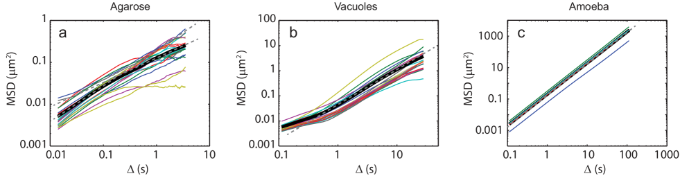
Figure 1: MSD analysis. (a) Time-averaged MSD (TA-MSD), Eq. (8) as a function of lag time $\Delta$ for 20 individual microsphere trajectories together with their ensemble average. (b) TA-MSD for 20 individual representative vacuole trajectories together with the ensemble average from 50 trajectories. (c) TA-MSD for four individual amoeba trajectories together with their ensemble average. In all three panels the thick black lines show the ensemble averages and the grey dashed lines show power law behaviour MSD $\sim\Delta^{\alpha}$.

Four individual amoeba trajectories, each consisting of 16,384 frames, were analysed in terms of their PSD. Short vacuole trajectories were discarded and 50 vacuoles trajectories, all from the same cell, were analysed. In order to avoid differences in trajectory lengths, only the first 2,048 frames in each vacuole trajectory were used in the analysis.

Mean squared displacement (MSD)

The time-averaged MSD of individual trajectories $X_{p}$, where $p$ is an appropriately discretized time variable, is defined as (see, e.g., Ref. pccp )

$$\overline{\delta^{2}(\Delta)}=\frac{1}{N-\Delta}\sum_{p=1}^{N-\Delta}\left(X_{p+\Delta}-X_{p}\right)^{2}.$$ (8)

This property was computed in MATLAB as a function of the lag time $\Delta$ for all analysed trajectories. The MSD of representative microspheres, amoeba, and vacuole trajectories along with their ensemble mean are shown in Fig. 1. The MSD from the analysed telomere trajectories were previously reported SW2017 . The anomalous exponent as obtained from the MSD is for microspheres $\alpha_{S}=0.87$ for short times and $\alpha_{L}=0.61$ for longer times (Fig. 1a); for telomeres $\alpha=0.5$ (see Ref. SW2017 ); for vacuoles $\alpha=1.33$ (Fig. 1b); and for amoeba $\alpha=1.97$ (Fig. 1c).

PSD analysis

Single- and two-component PSDs of individual trajectories (as defined in Eqs. (5) and (6), respectively), were obtained in MATLAB from the Fourier-transformed components $X_{t}^{(1)}$ and $X_{t}^{(2)}$ of three-dimensional trajectories. Care was taken that all trajectories of the same type included the same number of data points and the same frame rate.

For analysing the fluctuations of the PSD, i.e., to obtain the empirical distributions of the amplitudes of the PSD for sub- and super-diffusive cases, the gross scaling $1/f^{\beta}$ was obtained from the ensemble-averaged PSD, where $\beta=2H+1$ for the sub-diffusive cases (microspheres and telomeres) and $\beta=2$ for the super-diffusive ones (vacuoles). From these data sets we extracted values $A^{\prime}=S(f,T)f^{\beta}$ in the following frequency ranges: (i) $11\mathrm{Hz}<f<87\mathrm{Hz}$ for microspheres, (ii) $1\mathrm{Hz}<f<10\mathrm{Hz}$ for telomeres, and (iii) $1\mathrm{Hz}<f<5\mathrm{Hz}$ for vacuoles. We did not extract the fluctuations of the amoeba because only four trajectories were used. Then, we normalised the fluctuations according to $A=A^{\prime}/\langle A^{\prime}\rangle$. The same procedure was followed to obtain $B$ for the vacuoles. These data were then compared to the theoretical predictions as described in Sec. IV below.

Numerical algorithms

Numerical simulations of fBm are far more complicated than the ones used, for example, for a standard Brownian motion. FBm is not a Markov process and has long range correlations. In order to reproduce fBm numerically we use the exact Davies Harte Circulant method (see, e.g., Refs. DH ; WC ; DN ; D ; MD ). Due to the use of Fast Fourier Transform the required CPU time for reproducing a $T$ steps trajectory is of order $T\log(T)$ (and not of order $T^{2}$ as a naive approach would give). The Davies-Harte approach is a very powerful exact method, and for samples of the size we use its running time is comparable to the one of effective approximate methods D . We use trajectories of $T=2^{21}$ to $T=2^{23}$ discrete time steps. The total CPU time we have used for all the numerical runs that have been useful to prepare this work is of the order of few months of one core of Intel(R) Xeon(R) CPU E5-2620 0 $@$ 2.00GHz.

IV Analytical predictions

Our first step consists in calculating the moment-generating function $\Phi_{\lambda}$ of the $k$-component single-trajectory PSD (see Eq. (6)), defined in Eq. (7). We obtain (see SM for the details of the derivation)

$$\Phi_{\lambda}=\left[1+2\mu\lambda+\left(2-\gamma^{2}\right)\mu^{2}\lambda^{2}\right]^{-k/2},$$ (9)

where $\mu$ is the first moment of a single-component single-trajectory PSD, Eq. (2), $\sigma^{2}$ is the variance of this random variable, Eq. (3), and $\gamma=\sigma/\mu$ is the coefficient of variation of the PDF of a single-component single-trajectory PSD $S(f,T)$, Eq. (5). Inverting the Laplace transform with respect to $\lambda$ we readily obtain the PDF of $S_{k}(f,T)$,

$$P\left(S_{k}(f,T)=S\right)=\frac{\sqrt{\pi}}{2^{\frac{k-1}{2}}\Gamma\left(k/2\right)\sqrt{2-\gamma^{2}}\left(\gamma^{2}-1\right)^{\frac{k-1}{4}}}$$ (10)

$$\times \frac{S^{\frac{k-1}{2}}}{\mu^{\frac{k+1}{2}}}\exp\left(-\frac{1}{2-\gamma^{2}}\frac{S}{\mu}\right){\rm I}_{\frac{k-1}{2}}\left(\frac{\sqrt{\gamma^{2}-1}}{2-\gamma^{2}}\frac{S}{\mu}\right)\,,$$

where ${\rm I}_{\nu}(z)$ is the modified Bessel function of the $1$st kind. We emphasise that the expressions in Eqs. (9) and (10) are exact and hold for any $f$, $T$ and also for any value of the Hurst index $H$. We note that $\Phi_{\lambda}$ and $P\left(S_{k}(f,T)=S\right)$ are entirely defined by the first two moments of $S(f,T)$—and hence, all higher moments of the $k$-component single-trajectory PSD $S_{k}(f,T)$ can be expressed solely through the first two moments of $S(f,T)$. This is a direct consequence of the Gaussian nature of the parental process $X_{t}$. This suggests, in turn, that the expressions in Eqs. (9) and (10) may hold, in general, for arbitrary Gaussian processes, not necessarily for the fBm only. The dependence $\mu$, $\sigma^{2}$ and hence, of $\gamma$ on the characteristic parameters will depend, of course, on the case at hand.

For fBm processes, the exact dependence of $\mu$, $\sigma$ and, hence, of $\gamma$ on $f$ and $T$ for any value of $H\in(0,1)$ is presented in SM. Below we discuss their rather complex behavior focusing first on the coefficient of variation $\gamma$, which characterizes the effective broadness of the PDF in Eq. (10).

The coefficient of variation $\gamma$, which enters Eqs. (9) and (10), is a dimensionless numerical factor that depends on $f$ and $T$ only through the function $\omega=fT$. Figure 2 shows $\gamma$ as a function of $\omega$ for six different Hurst indices spanning the range $1/4\leq H\leq 7/8$. The behaviour of $\gamma$ has several characteristic features, which can be clearly observed in Fig. 2:
(i) In the limit $\omega\to 0$, the coefficient $\gamma$ tends to the universal value $\sqrt{2}$, regardless of the value of $H$. Next, $\gamma$ is an oscillatory function of $\omega$, and the oscillations are prominent at moderate values of $\omega$. In the limit $\omega\gg 1$ the oscillatory terms fade out and $\gamma$ is given by very simple asymptotic formula (see SM for derivation)

$$\gamma\sim\left[1+\left(1+c_{H}\omega^{1-2H}\right)^{-2}\right]^{1/2},$$ (11)

with $c_{H}=\Gamma\left(1+2H\right)\sin\left(\pi H\right)$. This asymptotic form is depicted by thin solid curves in Fig. 2.
(ii) We see that $\gamma\geq 1$, in the whole range of variation of $\omega$. This signifies that the standard deviation of the single-component single-trajectory PSD always exceeds its mean value. In consequence, the PDF in Eq. (10) is effectively broad and the analysis of the power spectrum using the standard ensemble-averaged PSD $\mu$ only is rather meaningless.
(iii) A most remarkable feature - rendering $\gamma$ a crucial and highly practical property for fBm-type processes - is that it offers the sought criterion for anomalous diffusion, since the values attained by $\gamma$ in the limit $\omega\to\infty$ are distinctly different: $\sqrt{2}$, $\sqrt{5}/2$, and $1$, independent of the exact value of $H$ but solely dependent on whether one has a superdiffusive ($H>1/2$), diffusive ($H=1/2$), or subdiffusive ($H<1/2$) behaviour, respectively. These analytical predictions are fully confirmed by numerical simulations for a number of $H$ values.

Before we proceed, it may be expedient to dwell some more on the last point. When dealing with particle-tracking experiments, one often observes values of $\alpha$ that are only slightly different from $1$. Consequently, in these cases, it is not obvious whether one is dealing with anomalous diffusion, or simply if the fitting of the curves started too early and includes transient behavior. On the other hand, the asymptotic value of $\gamma$ at large frequencies provides, in principle, an immediate answer to this question and reveals whether the underlying diffusion process is normal or anomalous. Such an unequivocal confirmation of anomalous diffusion can provide extremely valuable evidence to drive efforts into searching for microscopic mechanisms underlying the dynamics and lead eventually to a deeper comprehension of the processes in the system under study.

Note that here, however, we resorted to proof-of-concept numerical simulations, because the confirmation of this prediction requires a rather big statistical sample, which we were unable to create in current experimental analysis. We nonetheless perform such an analysis below in Sec. V (see Fig. 4): it appears to be instructive and shows that even a small sample containing only few tens of trajectories can provide a meaningful representation of the overall trend. Given the current rapid progress in single particle tracking techniques, sufficiently large experimental samples are certainly within reach.

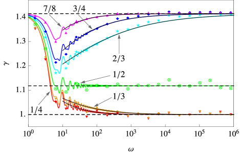
Figure 2: Coefficient of variation $\gamma$ as a function of $\omega=fT$. Colored solid curves represent exact values of $\gamma$ (arrows indicate the corresponding values of $H$), defined by Eq. (47) in the SM, while thin solid curves depict the asymptotic expression in Eq. (11). Horizontal dashed lines correspond to $\sqrt{2}$ (top), $\sqrt{5}/2$ (middle) and $1$ (bottom). Symbols represent numerical results averaged over $10^{4}$ realizations of trajectories consisting of $T=2^{23}$ discrete time steps.

Even though $\gamma$ allows finding whether the process is subdiffusive or superdiffusive, it does not permit one to deduce the value of the anomalous diffusion exponent $\alpha$. Below we discuss how one can find this further piece of the puzzle by analyzing the asymptotic behavior of the ensemble-averaged PSD $\mu$ and the corresponding limiting behavior of the PDF in Eq. (10). Consider first the case of subdiffusion ($H<1/2$). We suppose that $\omega$ is sufficiently large, such that $\gamma-1\leq\varepsilon$, where $\varepsilon$ is a small parameter. In virtue of relation (11) the above inequality holds for $\omega$ within the interval $\omega\in(\omega_{l}^{(\mathrm{sub})},\infty)$ where $\omega_{l}^{(\mathrm{sub})}=1/(2c_{H}\varepsilon)^{1/(1-2H)}$ (e.g., for $H=1/4$ and $\varepsilon=0.01$ one gets $\omega_{l}\approx 6.4\times 10^{3}$). In this limit, the denominator in Eq. (9) becomes a full square, i.e., $\Phi_{\lambda}\simeq\left[1+\mu\lambda\right]^{-k}$, with accuracy set by $\varepsilon$. This means, in turn, that the PDF of $S_{k}(f,T)$ becomes, up to terms of order of $\varepsilon$, the gamma distribution with shape parameter $k$ and scale parameter $\mu$. Consequently, in this case, the $k$-component single-trajectory PSD obeys the equality in distribution

$$\frac{S_{k}(f,T)}{\mu^{\mathrm{(sub)}}}\overset{d}{=}A+O(\varepsilon),$$ (12)

where the omitted terms are small in $\varepsilon$ and $A$ is a random numerical factor with distribution

$$P(A)=A^{k-1}\exp(-A)/\Gamma(k).$$ (13)

In the superdiffusive case ($H>1/2$), we again assume that $\omega$ is sufficiently large such that the inequality $\sqrt{2}-\gamma\leq\varepsilon$ holds. By virtue of relation (11), this is true when $\omega\in(\omega_{l}^{(\mathrm{sup})},\infty)$ with $\omega_{l}^{(\mathrm{sup})}=(2\sqrt{2}c_{H}/\varepsilon)^{1/(2H-1)}$ (e.g., for $H=3/4$ and $\varepsilon=0.01$, we have that $\omega_{l}^{(\mathrm{sup})}\approx 7.1\times 10^{4}$, i.e., a somewhat bigger value than the one in the subdiffusive case). In this limit the coefficient in front of the term quadratic in $\lambda$ in the denominator in Eq. (9), (i.e., $(2-\gamma^{2})$), is less than $\varepsilon$ such that $\Phi_{\lambda}\simeq\left[1+2\mu\lambda\right]^{-k/2}$ and, in turn, the PDF of $S_{k}(f,T)$ becomes the gamma distribution with scale $2\mu$ and shape parameter $k/2$. Consequently, the $k$-component single-trajectory PSD follows the equality in distribution

$$\frac{S_{k}(f,T)}{\mu^{\mathrm{(sup)}}}\overset{d}{=}2B+O(\varepsilon),$$ (14)

where $B$ is a random numerical factor with distribution

$$P(B)=B^{k/2-1}\exp(-B)/\Gamma(k/2).$$ (15)

Therefore, the equalities in Eqs. (12) and (14) suggest that for both the subdiffusive and superdiffusive cases the single-trajectory PSD should always be linearly proportional to its ensemble-average value $\mu$, (which incorporates the dependence on frequency), at large values of $\omega$. The proportionality factor is merely a random number with distribution given by Eqs. (13) or (15), which does not entail any additional dependence on $f$ or $T$.

Below we specify the spectral content of $\mu$. In the SM we show that for subdiffusive fBm at sufficiently large values of $T$ and $f$, $\mu$ has the scaling form

$$\mu^{\mathrm{(sub)}}=\frac{2c_{H}D}{f^{2H+1}}.$$ (16)

In the superdiffusive case $H>1/2$, at large $T$ and $f$,

$$\mu^{\mathrm{(sup)}}=\frac{2D}{f^{2}}T^{2H-1}+\frac{2c_{H}D}{f^{2H+1}}+o\left(1\right),$$ (17)

where the Landau symbol $o(1)$ states that the omitted terms vanish as $T\to\infty$. Result (17) unveils two remarkable features of the ensemble-averaged PSD in the superdiffusive case:
(i) First, regardless of the value of $H$, for large $T$, the frequency dependence has the universal $1/f^{2}$ form, precisely that of the PSD for standard Brownian motion. Therefore, experimental analyses of the frequency dependence of the PSD in the superdiffusive case may lead to the false conclusion that one deals with Brownian motion ($H=1/2$). Consequently, one should exercise care in interpreting data in this case: while Brownian motion has a PSD that scales as $1/f^{2}$, the observation of exclusively such a dependence does not guarantee that one indeed deals with Brownian motion.
(ii) Second, a crucial difference from Brownian motion is the dependence of the amplitude on the observation time $T$. This ageing behavior can be used to distinguish the $T$-independent PSD for Brownian motion from the superdiffusive case: $H$ can be deduced by analysing the spectrum at some fixed frequency given that one expects $S_{k}(f,T)\sim T^{2H-1}$.

Lastly, we show that the value of $H$ can be deduced from the spectrum evaluated at zero frequency,

$$S_{k}(f=0,T)=\frac{1}{T}\sum_{j=1}^{k}\left(\int^{T}_{0}X_{t}^{(j)}dt\right)^{2}\,,$$ (18)

which represents the sum (divided by $T$) of squared areas under the projections of the random curve $X_{t}$ on different axes. In the SM we show that the ensemble-averaged PSD at zero frequency is universally (for both subdiffusive and superdiffusive $H$) described by

$$\mu(f=0,T)=\frac{DT^{2H+1}}{(H+1)}\,,$$ (19)

(see also the result in Ref. satya with the reset rate set equal to zero). On the other hand, the variance of the single-trajectory PSD obeys (see SM), again for any $H$,

$$\sigma^{2}(f=0,T)=\frac{2D^{2}T^{4H+2}}{(H+1)^{2}}\,.$$ (20)

This signifies that the coefficient of variation $\gamma=\sqrt{2}$, regardless of the value of $H$, such that the PDF of $S_{k}(f=0,T)$ is the gamma distribution with scale $2\mu(f=0,T)$ and shape parameter $k/2$ for any $T$. In consequence, $S_{k}(f=0,T)$ obeys exactly the single-trajectory relation in Eq. (14) with the correction term $O(\varepsilon)$ identically equal to zero implying that the Hurst index can be deduced directly from the PSD at zero frequency.

Below we explore both possibilities to deduce $H$ from a single-trajectory data, taking advantage of the ageing behavior of $S_{k}(f,T)$ and of the dependence of the PSD at zero frequency on the observation time $T$.

V Comparison with experimental and numerical data

We tested our predictions for the PSD of single trajectories in four different experimental data sets and multiple numerical simulations. The experimental data consist of two systems exhibiting subdiffusive behavior and two systems exhibiting superdiffusion. For subdiffusive dynamics, we analysed the motion of 50-nm microspheres in agarose gels and telomeres in the nucleus of mammalian cells SW2017 . For superdiffusive behaviour, we studied the motion of live amoeba and their intracellular vacuoles. Representative MSD of individual trajectories in all these systems are presented in Fig. 1 along with their respective averages of the time-averaged MSDs. Examples of PSDs of the single trajectories are shown in Figs. 3a-d.

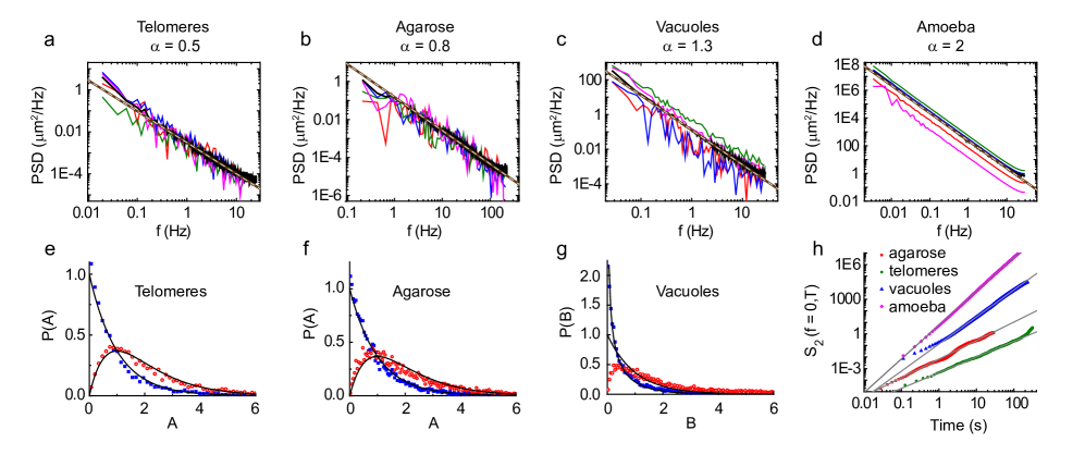
Figure 3: Power spectrum analysis of experimental data sets. (a-d) PSD of representative trajectories along with the ensemble-averaged PSD for telomeres in the nucleus of HeLa cells, 50-nm microspheres in 1.5% agarose gel, intracellular vacuoles within amoeba, and the motion of amoeba. The dashed thick lines show the $1/f^{1.49}$ trend for panel (a), $1/f^{1.76}$ for panel (b) and $1/f^{2}$ for panels (c) and (d). In each case, the PSDs of four trajectories are presented (log-sampled with a factor 1.1 for clarity) together with the ensemble-averaged PSD (thicker black lines, $n=19,20,50,$ and $4$ trajectories for telomeres, microspheres, vacuoles, and amoeba, respectively). (e-g) Distribution of amplitudes of the PSD for one and two components. (h) PSD evaluated at zero frequency. The zero frequency spectra are shifted for clarity and displayed together with the fitted power-law functions (grey solid lines). The experimental results throughout agree excellently with the theoretical predictions.

The time-averaged MSDs of telomeres scale with an exponent $\alpha=0.5$, (i.e., $H=0.25$) for short and intermediate times SW2017 , predicting a PSD $S(f,T)\sim A/f^{1.5}$. As shown in Fig. 3a, the individual trajectories agree with this prediction and the ensemble-averaged PSD from 19 trajectories yields $\mu^{(\mathrm{sub})}\sim 1/f^{1.49}$. We also show that the experimentally observed fluctuations in the PSDs remarkably confirm the predicted universal distribution Eq. (13) for both one- and two-components PSDs, i.e., for $k=1$ and $k=2$, respectively (Fig. 3e). Similar agreements are found for the motion of $50$-nm microspheres in $1.5\%$ agarose gel. As shown in Fig. 1a, the MSD of these particles scales with an exponent $\alpha=0.87$ ($H=0.43$) for short times and $\alpha=0.61$ ($H=0.30$) for long times. The PSD yields $\mu^{(\mathrm{sub})}\sim 1/f^{1.76}$ (Fig. 3b), and the PSD fluctuations also follow closely a gamma distribution (Fig. 3f) as predicted by Eq. (13).

The motion of amoebae and their intracellular vacuoles are good examples of superdiffusive dynamics. Intracellular vacuoles are subdiffusive at short lag times and superdiffusive with $\alpha=1.33$ at long lag times (Fig. 1b). This behaviour is typical of active motion in the cytoplasm ActiveMotion . Interestingly, the MSDs of the centre of mass of the investigated amoebae show almost ballistic motion with $\alpha=1.97$ (Fig. 1c). The PSDs of the motion of both the amoebae and the vacuoles therein, clearly show the predicted deceptive $1/f^{2}$ behavior (Figs. 3c and d). The distribution of the PSD amplitudes is also shown for the vacuoles in Fig. 3g together with the predicted gamma distributions, Eq. (15), revealing an excellent agreement with the latter for $k=1$. The discrepancy with our two-component analytical prediction for small $B$-values is likely associated with small amplitude antipersistent motion of the vacuoles, as is evident from the trajectories.

In Fig. 3h we present the averaged spectra at zero frequency for both subdiffusive and superdiffusive cases ( see eqs. (19) and (20) in Sec. IV). We used $19$, $20$, $50$ and $4$ trajectories for the telomeres, microspheres, vacuoles and amoeba, respectively, to get directly the Hurst exponents: $H=0.30$, $0.18$, $0.67$ and $1.92$. Despite the small sizes of our statistical samples, the obtained values of $H$ agree well with the values deduced from the corresponding MSDs.

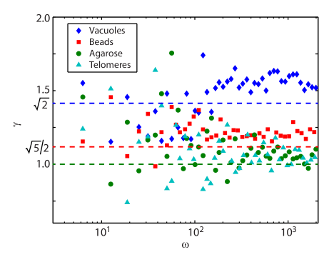
Figure 4: Coefficient of variation $\gamma$ as a function of $\omega=fT$ in small statistical samples of experimental data. Dashed horizontal lines highlight the analytical predictions made in Sec. IV with blue, red, and green indicating the values $\gamma=\sqrt{2}$ (superdiffusive fBm), $\gamma=\sqrt{5}/2$ (standard Brownian motion diego ), and $\gamma=1$ (subdiffusive fBm), respectively. Symbols represent the values of $\gamma$ drawn from experiments. Blue diamonds: vacuoles ($50$ trajectories); red squares: $1.2$-$\mu$m beads in aqueous solution ($150$ trajectories) diego ; green circles: $50$-nm microspheres in agarose hydrogel ($20$ trajectories); and cyan triangles: telomeres in the nucleus of mammalian cells ($19$ trajectories).

We revisit next the behavior of the coefficient of variation $\gamma$ of the single-trajectory PDF (see Fig. 2) and address the question whether meaningful information can already be drawn from small statistical samples of experimental data. In Fig. 4 we plot the value of $\gamma$ as a function of $\omega=fT$ obtained from only $19$ experimentally recorded trajectories of telomeres, $20$ trajectories of microspheres in agarose hydrogels and $50$ intracellular vacuole trajectories, as well as from a larger number of trajectories ($150$) of micrometer-sized beads in an aqueous solution diego . The microspheres in aqueous solution provide an excellent example of standard Brownian motion, i.e., $H=0.5$. One observes that, indeed, in the large-$\omega$ limit, $\gamma$ converges to distinctly different values for superdiffusion, normal diffusion and subdiffusion cases. For vacuoles, at large $\omega$, the coefficient of variation $\gamma$ is observed to converge to $1.55\pm 0.01$, for Brownian motion (beads in aqueous solution), it is observed to converge to $1.21\pm 0.01$, for telomeres to $1.05\pm 0.01$ and for the microspheres in agarose gels to $1.07\pm 0.01$. In line with our analytical prediction of a universal value of $\gamma$ for subdiffusive fBm, the obtained values for telomeres and microspheres are very close to each other. Overall, the experimentally determined values for $\gamma$ are only about 10% larger than our analytical predictions ($\sqrt{2}\approx 1.41$ for vacuoles, $\sqrt{5}/2\approx 1.12$ for beads in aqueous solution diego , and $1$ for telomeres and microspheres). Given the small size of the statistical sample, we consider such a favorable agreement quite remarkable. In comparison, the perfect agreement of our predictions with $\gamma$ values from fBm simulations (cf. Fig. 2) rather represents an exceptional situation due to the big statistical sample ($10^{4}$ trajectories). Moreover, in experiments many different, sometimes uncontrollable factors, e.g. detector noise, may come into play which leads to an increasing variance of the single-trajectory PSD and hence to elevated values of $\gamma$. We plan to examine this important aspect in more detail in our future work.

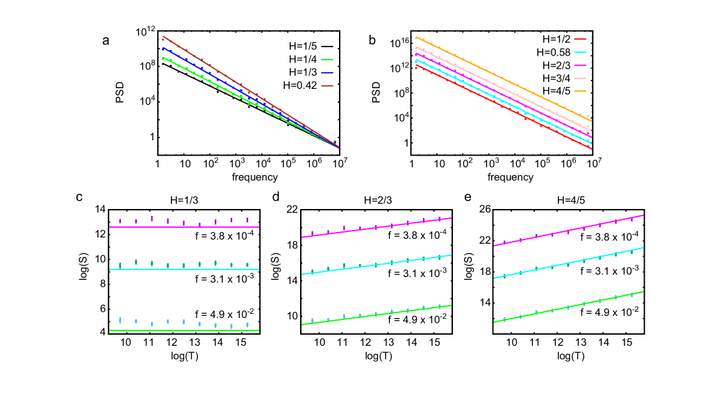
Figure 5: Numerical confirmation of our theoretical predictions. (a) Frequency dependence of a single-trajectory PSD in the subdiffusive case (Eqs. (12) and (16)) for $H=0.42,1/3,1/4$, and $H=1/5$, averaged over $10$ realisations. Straight lines have slope $-(2H+1)$, as shown in Eq. (16). The symbols represent the results of numerical simulations. (b) Deceptive $1/f^{2}$-dependence (Eq. (17)) in the superdiffusive case. Symbols represent results of numerical simulations for individual trajectories averaged over $10$ realisations. (c) Apparent independence of a single-trajectory PSD in the subdiffusive case on the observation time for sufficiently large $T$. (d-e) Ageing behavior of a single-trajectory PSD in the superdiffusive case for three different values of the frequency. Straight lines have slopes $2H-1$ as shown in Eq. (17). Symbols represent numerical results averaged over $50$ realisations.

We further performed extensive analyses of single-trajectory PSDs for different values of $H$ using numerical simulations. Figures 5a and b show the results for single-trajectory PSDs as a function of the frequency (for sufficiently large $T$) for different values of $H$ between $1/5$ and $4/5$. Namely, the subdiffusive cases ($H<1/2$) are shown in Fig. 5a and other cases ($H>1/2$) are shown in Fig. 5b. One observes excellent agreement between the predicted behaviour, Eqs. (12) and (16), and the numerics even for a small statistical sample consisting of $10$ realisations. In Fig. 5c we also demonstrate that the single-trajectory PSD for a specific subdiffusive case ($H=1/3$) is not ageing. On the other hand, Figs. 5e and f illustrate the ageing behavior of a single-trajectory PSD for $H=2/3$ and $4/5$, at three fixed frequencies. Here, the straight lines indicate the predicted ageing dependence $T^{2H-1}$, Eq. (17), while the symbols represent the results of numerical simulations averaged over $50$ realisations. We again observe a perfect agreement with our theoretical predictions.

VI Discussion

In summary, we here combined theoretical, numerical and experimental analyses to provide a comprehensive answer to the conceptually and practically important question: which information can be reliably obtained from the spectral content of a single realisation of naturally occurring anomalous-diffusion processes. Given the widespread occurrence of $1/f$-type of spectra in the analysis of experimental systems and signals across almost every field of physics, such an analysis is very pertinent. Focusing on a wide class of such processes—the so-called fractional Brownian motion—we derived exactly the distribution of a single-trajectory power-spectral density (PSD) and analyzed its asymptotic forms for both subdiffusive and superdiffusive dynamics. On this basis, we unveiled several striking features:
(i) At a fixed observation time and in the limit of high frequencies, this distribution reduces to simple forms with a unique scaling given by the ensemble-averaged PSD, which incorporates the full dependence on $f$ and $T$. As a consequence, one expects that for an arbitrary realization of the process a single-trajectory PSD should exhibit the same large-$f$ dependence as a traditional ensemble-averaged PSD.
(ii) Our experiments and numerical simulations impressively evidence that this is indeed the case for both super- and subdiffusive fBm-type processes. For subdiffusive processes, the exponent characterising the spectrum is equal to $2H+1$ and hence, the anomalous diffusion exponent can be obtained by evaluating the slope of the PSD. For superdiffusive processes, in contrast, the exponent is deceptively universal and equal to two, which can lead to the false conclusion that one deals with ordinary Brownian motion, while in reality the process is superdiffusive. We find this prediction particularly important since it will permit to avoid a misinterpretation of experimental results.
(iii) For superdiffusive processes the amplitude of the PSD is ageing, i.e., dependent on the observation time. However, it is difficult to observe this dependence on a single trajectory since the $T$-dependence is weaker than the large fluctuations between nearby frequencies. Here, a statistical sample (comprising, however, only $50$ trajectories) was used in order to observe the ageing trend and to extract the value of the anomalous diffusion exponent from the ageing behavior.
(iv) We showed that the coefficient of variation $\gamma$ of a single-trajectory PSD provides a novel criterion for anomalous diffusion. For fBm, its large-$f$ form assumes only three different values, depending on whether we observe subdiffusion, normal diffusion, or superdiffusion. Our analytical predictions are in a perfect agreement with the results of numerical simulations for a representative statistical sample ($10^{4}$ trajectories), but are also in line with the experimental results, obtained from a fairly small statistical sample ($19$ to $50$ trajectories).
(v) Lastly, our theoretical, numerical and experimental analysis shows unequivocally that the coefficient of variation always exceeds the value $1$, meaning that the standard deviation of a single-trajectory PSD is generically bigger than its mean value. In standard nomenclature of the statistical analysis, the distributions which possess such a property are considered to be effectively broad. This implies that the analysis of the spectral content of individual trajectories in terms of only the ensemble-averaged PSD has limited meaning, which justifies completely our quest for the full PDF of this important characteristic property.

To conclude, from an experimental perspective, our results serve as a reliable framework in the interpretation of noisy data obtained from a single trajectory - it has become routine to garner few individual particle trajectories of impressive length in the wake of superresolution microscopy and super- computing. In perspective, our results will thus play an important role in extracting more physical information from them.

Finally, we remark that especially in the complex environment of biological cells, where a vast array of specific and non-specific interactions transpire, fBm does not account, of course, for all possible types of observed anomalous diffusions. Therefore, additional stochastic mechanisms may be superimposed, such as short-time or even simultaneous scale-free trapping time dynamics lene ; tabei ; weigel ; weron17 . In other instances, fBm may be tempered or there may occur dynamical transitions between different types of fBm igor ; daniel . Extensions of our analysis over other possible kinds of anomalous diffusion, such as the fBm models with dynamical transitions igor , “diffusing diffusivity” models chechkin , scaled Brownian motion sbm , or continuous-time random walks with a broad distribution of waiting times scher are necessary in order to get a full understanding of the behavior of the PSD in experimentally relevant systems. We believe that our work presents an important first step towards such an understanding and will prompt a systematic case-by-case analysis.

Authors contributions

D.K. and X.X. performed experimental single-trajectory analyses of anomalous diffusion of microspheres in agarose hydrogels, N.L. and C.S-U. studied dynamics of amoebae and their intracellular vacuoles, while L.S. and M.W. performed particle-tracking experiments with telomeres in the nucleus of mammalian cells. D.K. and M.W. analysed the power-spectra of individual experimental trajectories. E.M. performed numerical analysis of power spectral densities of fractional Brownian motion. R.M., G.O. and A.S. performed all analytical calculations. D.K., R.M., E.M., G.O., C.S-U. and M.W. have equally contributed to writing the paper.

Conflict of interests

The authors declare no conflict of interests.

References

- (1) M. P. Norton and D. G. Karczub, Fundamentals of noise and vibration analysis for engineers, (Cambridge University Press, Cambridge UK, 2003).
- (2) R. Voss and J. Clarke, -noise in music and speech, Nature 258, 31 (1975).
- (3) H. Hennig, R. Fleischmann, A. Fredebohm, Y. Hagmayer, J. Nagler, A. Witt, F. J. Theis, and T. Geisel, The nature and perception of fluctuations in human musical rhythms, PLoS ONE 6, e26457 (2011).
- (4) R. O. Weber and P. Talkner, Spectra and correlations of climate data from days to decades, J. Geophys. Res. 106, 20131 (2001).
- (5) A. Sornette and D. Sornette, Self-organized criticality and earthquakes, Europhys. Lett. 9. 197 (1989).
- (6) J. W. Kirchner, X. Feng, and C. Neal, Fractal stream chemistry and its implications for containment transport in catchments, Nature 403, 524 (2000).
- (7) A. A. Balandin, Low-frequency noise in graphene devices, Nat. Nanotechnol. 8, 54 (2013).
- (8) P. A. Frantsuzov, S. Volkán-Kacsó, and B. Jank, Universality of the fluorescence intermittency in nanoscale systems: experiment and theory, Nano Lett. 13, 402 (2013).
- (9) D. Krapf, Nonergodicity in nanoscale electrodes, Phys. Chem. Chem. Phys. 15, 459 (2013).
- (10) S. N. Majumdar and G. Oshanin, Spectral content of fractional Brownian motion with stochastic reset, J. Phys. A: Math. Theor. 51, 435001 (2018).
- (11) O. Bénichou, P. L. Krapivsky, C. Mejía-Monasterio, and G. Oshanin, Temporal correlations of the running maximum of a Brownian trajectory, Phys. Rev. Lett. 117, 080601 (2016).
- (12) E. Marinari, G. Parisi, D. Ruelle, and P. Windey, Random Walk in a Random Environment and Noise, Phys. Rev. Lett. 50, 1223 (1983).
- (13) D. S. Dean, E. Marinari, A. Iorio, and G. Oshanin, Sample-to-sample fluctuations of power spectrum of a random motion in a periodic Sinai model, Phys. Rev. E 94, 032131 (2016).
- (14) M. Zorkot, R. Golestanian, and D. J. Bonthuis, The power spectrum of ionic nanopore currents: The role of ion correlations, Nano Lett. 16, 2205 (2016).
- (15) K. Nørregaard, R. Metzler, C. M. Ritter, K. Berg-Sørensen, and L. B. Oddershede, Manipulation and Motion of Organelles and Single Molecules in Living Cells, Chem. Rev. 117, 4342 (2017).
- (16) D. B. Kemp, K. Eichenseer, and W. Kiessling, Maximum rates of climate change are systematically underestimated in the geological record, Nat. Commun. 6, 8890 (2015).
- (17) B. Tóth, Y. Lempérière, C. Deremble, J. de Lataillade, J. Kockelkoren, and J.-P. Bouchaud, Anomalous price impact and the critical nature of liquidity in financial markets, Phys. Rev. X 1, 021006 (2011).
- (18) M. Niemann, H. Kantz, and E. Barkai, Fluctuations of noise and the low-frequency cutoff paradox, Phys. Rev. Lett. 110, 140603 (2013).
- (19) S. Sadegh, E. Barkai, and D. Krapf, noise for intermittent quantum dots exhibits non-stationarity and critical exponents, New J. Phys. 16, 113054 (2014).
- (20) M. Weiss, Single-particle tracking data reveal anticorrelated fractional Brownian motion in crowded fluids, Phys. Rev. E 88, 010101 (2013).
- (21) L. Li, E. C. Cox, and H. Flyvbjerg, ’Dicty dynamics’: Dictyostelium motility as persistent random motion, Phys. Biol. 8, 046006 (2011).
- (22) J. N. Pedersen, L. Li, C. Grâdinaru, R. H. Austin, E. C. Cox, and H. Flyvbjerg, How to connect time-lapse recorded trajectories of motile microorganisms with dynamical models in continuous time, Phys. Rev. E 94, 062401 (2016).
- (23) D. Krapf, E. Marinari, R. Metzler, G. Oshanin, X. Xu, and A. Squarcini, Power spectral density of a single Brownian trajectory: what one can and cannot learn from it, New J. Phys. 20, 023029 (2018).
- (24) N. D. Schnellbächer and U. S. Schwarz, The power of a single trajectory, New J. Phys. 20, 031001 (2018).
- (25) E. Frey and K. Kroy, Brownian motion: a paradigm of Soft Matter and biological physics, Ann. Phys. 14, 20 (2005).
- (26) C. Di Rienzo, V. Piazza, E. Gratton, F. Beltram, and F. Cardarelli, Probing short-range protein Brownian motion in the cytoplasm of living cells, Nat. Commun. 5, 5891 (2014).
- (27) J.-H. Jeon, V. Tejedor, S. Burov, E. Barkai, C. Selhuber-Unkel, K. Berg-Sørensen, L. Oddershede, and R. Metzler, In vivo anomalous diffusion and weak ergodicity breaking of lipid granules, Phys. Rev. Lett. 106, 048103 (2011).
- (28) S. A. Tabei, S. Burov, H. Y. Kim, A. Kuznetsov, T. Huynh, J. Jureller, L. H. Philipson, A. R. Dinner, and N. F. Scherer, Intracellular transport of insulin granules is a subordinated random walk, Proc. Natl. Acad. Sci. U.S.A. 110, 4911 (2013).
- (29) J.-H. Jeon, N. Leijnse, L. Oddershede, and R. Metzler, Anomalous diffusion and power-law relaxation in wormlike micellar solution, New J. Phys. 15, 045011 (2013).
- (30) J. Szymanski and M. Weiss, Elucidating the origin of anomalous diffusion in crowded fluids, Phys. Rev. Lett. 103, 038102 (2009).
- (31) I. Bronshtein, E. Kepten, I. Kanter, S. Berezin, M. Lindner, A. B. Redwood, S. Mai, S. Gonzalo, R. Foisner, Y. Shav-Tal, and Y. Garini, Loss of lamin A function increases chromatin dynamics in the nuclear interior, Nat. Commun. 6, 8044 (2015).
- (32) S. Havlin and D. ben-Avraham, Diffusion in disordered media, Adv. Phys. 36, 695 (1987).
- (33) G. Afek, J. Coslovsky, A. Courvoisier, O. Livneh, and N. Davidson, Observing power-law dynamics of position-velocity correlation in anomalous diffusion, Phys. Rev. Lett. 119, 060602 (2017).
- (34) D. Krapf, Mechanisms underlying anomalous diffusion in the plasma membrane, Curr. Top. Membr. 75, 167 (2015).
- (35) J.-H. Jeon, M. Javanainen, H. Martinez-Seara, R. Metzler, and I. Vattulainen, Protein crowding in lipid bilayers gives rise to non-Gaussian anomalous lateral diffusion of phospholipids and proteins, Phys. Rev. X 6, 021006 (2016).
- (36) R. Metzler, J.-H. Jeon, and A. G. Cherstvy, Non-Brownian diffusion in lipid membranes: experiments and simulations, Biochim. Biophys. Acta - Biomembranes 1858, 2451 (2016).
- (37) S. Sadegh, J. L. Higgins, P. C. Mannion, M. M. Tamkun, and D. Krapf, Plasma membrane is compartmentalized by a self-similar cortical actin meshwork, Phys. Rev. X 7, 011031 (2017).
- (38) C. K. Peng, J. Mietus, J. M. Hausdorff, S. Havlin, H. E. Stanley, and A. L. Goldberger, Long-range anticorrelations and non-Gaussian behavior of the heartbeat, Phys. Rev. Lett. 70, 1343 (1993).
- (39) C.-K. Peng, S. V. Buldyrev, A. L. Goldberger, S. Havlin, F. Sciortino, M. Simons, and H. E. Stanley, Long-range correlations in nucleotide sequences, Nature 356, 168 (1992).
- (40) A. W. Rempel, E. D. Waddington, J. S. Wettlaufer, and M. G. Worster, Possible displacement of the climate signal in ancient ice by premelting and anomalous diffusion, Nature 411, 568 (2001).
- (41) B. B. Mandelbrot and J. W. van Ness, Fractional Brownian motions, fractional noises and applications, SIAM Rev. 10, 422 (1968).
- (42) R. Metzler, J.-H. Jeon, A. G. Cherstvy, and E. Barkai, Anomalous diffusion models and their properties: non-stationarity, non-ergodicity, and ageing at the centenary of single particle tracking, Phys. Chem. Chem. Phys. 16, 24128 (2014).
- (43) I. Goychuk, Viscoelastic subdiffusion: generalized Langevin equation approach, Adv. Phys. 150, 187 (2012).
- (44) J. F. Reverey, J. -H. Jeon, H. Bao, M. Leippe, R. Metzler, and C. Selhuber-Unkel, Superdiffusion dominates intracellular particle motion in the supercrowded space of pathogenic Acanthamoeba castellanii, Sci. Rep. 5, 11690 (2015).
- (45) S. C. Weber, A. J. Spakowitz, and J. Theriot, Bacterial chromosomal loci move subdiffusively through a viscoelastic cytoplasm, Phys. Rev. Lett. 104, 238102 (2010).
- (46) G. R. Kneller, K. Baczynski, and M. Pasenkiewicz-Gierula, Consistent picture of lateral subdiffusion in lipid bilayers: Molecular dynamics simulation and exact results, J. Chem. Phys. 135, 141105 (2011).
- (47) J.-H. Jeon, H. Martinez-Seara Monne, M. Javanainen, and R. Metzler, Lateral motion of phospholipids and cholesterols in a lipid bilayer: anomalous diffusion and its origins, Phys. Rev. Lett. 109, 188103 (2012).
- (48) M. Di Pierro, D. A. Potoyan, P. G. Wolynes, and J. N. Onuchic, Anomalous diffusion, spatial coherence, and viscoelasticity from the energy landscape of human chromosomes, Proc. Natl. Acad. Sci. U.S.A. 115, 7753 (2018).
- (49) K. Burnecki, E. Kepten, J. Janczura, I. Bronshtein, Y. Garini, and A. Weron,Universal algorithm for identification of fractional Brownian motion. A case of telomere subdiffusion, Biophys. J. 103, 1839 (2012).
- (50) D. Ernst, M. Hellmann, J. Köhler, and M. Weiss, Fractional Brownian motion in crowded fluids, Soft Matter 8, 4886 (2012).
- (51) M. R. Shaebani, Z. Sadjadi, I. M. Sokolov, H. Rieger, and Ludger Santen, Anomalous diffusion of self-propelled particles in directed random environments, Phys. Rev. E 90, 030701(R) (2014).
- (52) D. Molina-Garcia, T. Sandev, H. Safdari, G. Pagnini, A. Chechkin, and R. Metzler, Crossover from anomalous to normal diffusion: truncated power-law noise correlations and applications to dynamics in lipid bilayers, New J. Phys. 20, 103027 (2018).
- (53) J.-H. Jeon, A. V. Chechkin, and R. Metzler, First passage behaviour of fractional Brownian motion in two-dimensional wedge domains, Europhys. Lett. 94, 20008 (2011).
- (54) C. Gosse and V. Croquette, Biophys. J. 82, 3314 (2002).
- (55) L. Stadler and M. Weiss, Non-equilibrium forces drive the anomalous diffusion of telomeres in the nucleus of mammalian cells, New J. Phys. 19, 113048 (2017).
- (56) R. B. Davies and D. S. Harte, Tests for Hurst Effect, Biometrika 74, 95 (1987).
- (57) A. Wood and G. Chan, Simulation of Stationary Gaussian Processes in , J. Comput. Graph. Stat. 3, 409 (1994).
- (58) C. R. Dietrich and G. N. Newsam, Fast and Exact Simulation of Stationary Gaussian Processes through Circulant Embedding of the Covariance Matrix, SIAM J. Sci. Comput. 18, 1088 (1997).
- (59) T. Dieker, Simulation of Fractional Brownian Motion, PhD Thesis, CWI, Amsterdam, and University of Twente, Enschede, The Netherlands, April 2002, and revised version from 2004.
- (60) M. Mandjes and T. Dieker, On Spectral Simulation of Fractional Brownian Motion, Probab. Eng. Inf. Sci. 17, 417 (2003).
- (61) P. Bursac, G. Lenormand, B. Fabry, M. Oliver, D. A. Weitz, V. Viasnoff, J. P. Butler, and J. J. Fredberg, Cytoskeletal remodelling and slow dynamics in the living cell, Nat. Mater. 4, 557 (2005).
- (62) A. V. Weigel, B. Simon, M. M. Tamkun, and D. Krapf, Ergodic and nonergodic processes coexist in the plasma membrane as observed by single-molecule tracking, Proc. Natl. Acad. Sci. U.S.A. 108, 6438 (2011).
- (63) A. Weron, K. Burnecki, E. J. Akin, L. Solé, M. Balcerek, M. M. Tamkun, and D. Krapf, Ergodicity breaking on the neuronal surface emerges from random switching between diffusive states, Sci. Rep. 7, 5404 (2017).
- (64) A. V. Chechkin, F. Seno, R. Metzler, and I. M. Sokolov, Brownian yet non-Gaussian diffusion: from superstatistics to subordination of diffusing diffusivities, Phys. Rev. X 7, 021002 (2017).
- (65) J-.H. Jeon, A. V. Chechkin, and R. Metzler, Scaled Brownian motion: a paradoxical process with a time dependent diffusivity for the description of anomalous diffusion, Phys. Chem. Chem. Phys. 16, 15811 (2014).
- (66) H. Scher and E. W. Montroll, Anomalous transit-time dispersion in amorphous solids, Phys. Rev. B 12, 2455 (1975).