Effective bandwidth of non-Markovian packet traffic

Abstract

We demonstrate the application of recent advances in statistical mechanics to a problem in telecommunication engineering: the assessment of the quality of a communication channel in terms of rare and extreme events. In particular, we discuss non-Markovian models for telecommunication traffic in continuous time and deploy the “cloning” procedure of non-equilibrium statistical mechanics to efficiently compute their effective bandwidths. The cloning method allows us to evaluate the performance of a traffic protocol even in the absence of analytical results, which are often hard to obtain when the dynamics are non-Markovian.

I Introduction

Natural systems made of many coupled components, ranging from ideal gases to living organisms and their communities, have long been of interest to scientists. Recently, by contrast, some of the most studied complex systems have been man-made, for instance telecommunication networks, transport infrastructures, and financial markets. The methods used to approach these technological systems are similar to those used in natural sciences. Indeed, at a sensible level of detail, the system properties appear as random variables, and the scientific effort is directed towards the quantification of such randomness, as well as of its effects. More specifically, in telecommunication engineering, we are interested in relating the elementary (“microscopic”) description of a telecommunication network in terms of packets and servers, to a perceivable (“macroscopic”) quantity, such as the service that is effectively available to the final user. Such a programme looks very similar to the one that led to the the development of statistical mechanics, where macroscopic observables (such as density and energy) are defined based on microscopic modelling.

Studies comparing communication networks and many-body physical systems are well-represented in the literature DeMartino2009 ; DeMartino2009a ; Chernyak2010 and it is now well understood that the analogies are based on the underlying mathematics of stochastic processes and large deviation theory Touchette2009 . This paper is built around the less well-known notion of effective bandwidth (EB), which has been introduced in the 90s to weight the effects of large deviation events in resource allocation Kelly1996 , (see also the more recent reference books Gautam2012 ; Srikant2013 ; Kelly2014 ; Larsson2014 ). It is worth noting that the efficient numerical evaluation of rare events is central within such a context, as in the real world a suitable amount of resources must be allocated even in the absence of analytical solutions for the probability of potentially disruptive rare events Heidelberger1995 ; Reijsbergen2012 ; Chang1994 . To do so, we choose a tool from non-equilibrium statistical mechanics, viz., the “cloning” method Giardina2011 . We are here particularly interested in systems with non-Markovian dynamics (relevant to real-world applications as well as statistical mechanics advances) and so we exploit a recent implementation of cloning for non-Markovian processes Cavallaro2016 .

The text is organised as follows. In section II some basic concepts from queuing theory are introduced to set the stage for the following sections. In section III we present, motivate, and review the notion of EB, which is connected to a large deviation analysis of the net load. In sections IV, V, and VI we analyse Markovian and non-Markovian models of packet traffic modulated by an underlying stochastic process. The cloning method is used to numerically compute their EBs. In particular, while sections IV and V deal with classic teletraffic toy models whose EBs are known analytically, in section VI we explore numerically the case of a modified non-Markovian two-phase process, observing that the EB increases as the dispersion of the phase lengths increases. Significantly, this leads to the observation that the EB in the new model can be adjusted by tuning the traffic parameters, whilst maintaining a fixed mean traffic rate. We conclude with a discussion in section VII.

II Net load, bandwidth, and their bounds

In a queuing network, we have a number of servers that exchange packets or customers. When a collection of packets leaves a server to reach another one, we say that a communication channel has been established between the two servers. In such a channel, we denote the random amount of work brought by customers passing through the channel during the interval $[0,t)$ as $X(t)$. This can be described as the integral over $[0,t)$ of a process $\mathrm{x}(t)$, which can be a “point” process (thought of as a series of random events describing customers – or particles – feeding one of the servers), or a “fluid”/“piece-wise deterministic” process (supplied continuously and deterministically between random times). We will not deal with a third possibility where the instantaneous work is supplied continuously and stochastically; however, many considerations in this paper arguably apply also to such a case. Similarly, we consider the amount of work $Y(t)$ that the receiving server is able to perform during the same amount of time, which is the integral over $[0,t)$ of another point or fluid process $\mathrm{y}(t)$. It is of central importance here that $X(t)$ and $Y(t)$ are assumed to be time-extensive, so that they play the role of integrated currents in standard interacting particle systems Chernyak2010 . Indeed, such a setting is quite general. For example, in the context of economics, $X(t)$ and $Y(t)$ can describe the total production and demand, respectively. It is also convenient to introduce the quantity $W(t)=X(t)-Y(t)$, which we refer to as the net load, and its derivative $\mathrm{w}(t)$.

Figure 1 (left panels) shows an example of such a setting when both $X(t)$ and $Y(t)$ are point processes. In this case, $W(t)$ has increments at the instants $(t_{1},t_{2},\ldots,t_{n})$, with $0\leq t_{1}\leq\ldots\leq t_{n}<t$, when discrete arrival or service events occur.

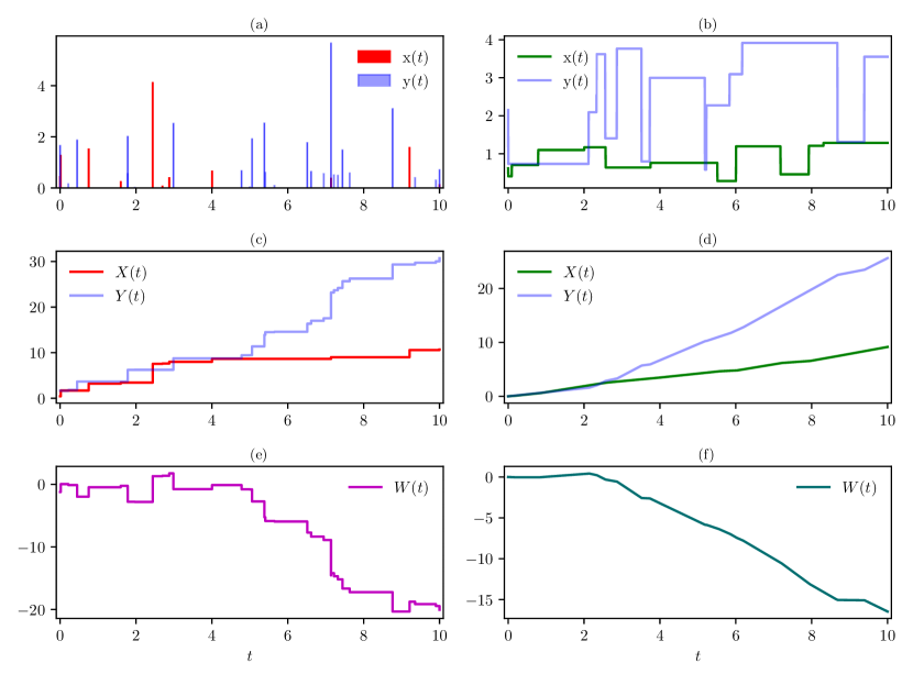
Figure 1: Left and right panels show example settings for point and fluid net loads, respectively. a) $\mathrm{x}(t)$ and $\mathrm{y}(t)$ represent discrete arrival and attempted service events, respectively. b) Both request $\mathrm{x}(t)$ and service $\mathrm{y}(t)$ are carried out continuously in time. The supply laws change at random time points, but are constant otherwise. c) and d) $X(t)$ is the total amount of work (e.g., customers to be served) requested during the interval $[0,t)$, while $Y(t)$ is the service that can be provided during the same amount of time. e) and f) Resulting outcomes of the net-load processes $W(t)=X(t)-Y(t)$.

‘ If $\mathrm{x}(t)$ or $\mathrm{y}(t)$ is fluid, then $W(t)$ increases or decreases deterministically between the random times $(t_{1},t_{2},\ldots,t_{n})$. This is illustrated in figure 1 (right panels). Obviously, it is possible to combine fluid and point processes.

In all the previous cases, the arrival, the service, and the net load can be regarded as driven by an underlying random process, which influences or modulates their evolution in a point-wise or piecewise-deterministic fashion. Conversely, the load itself has no influence on the modulating random process. More specifically, in a point process, increments occur at the random times $t_{i}$, $i=1,2,\ldots,n$, and their frequency and magnitude $\theta_{t_{i}}$ can be thought of as being dictated by the modulating random process. On the other hand, in a fluid process, the $t_{i}$s correspond to the transition times of the underlying process and at the end of an interval between two consecutive transition times $t_{i}$ and $t_{i+1}$ the net load has increased by an amount that depends on $(t_{i+1}-t_{i})$; for simplicity, we assume that the fluid rate is constant between transition times and the load increase is $(t_{i+1}-t_{i})\theta_{t_{i}}$. To maintain generality, we refer to all types of increment as $\Theta_{i}$.

We require that the limits $\bar{x}=\lim_{t\to\infty}X(t)/t$ and $\bar{y}=\lim_{t\to\infty}Y(t)/t$ exist, and we refer to the condition $\bar{x}<\bar{y}$ as stability, which implies that $W(t)/t$ concentrates around a negative value $\bar{w}=\bar{x}-\bar{y}$ as $t\to\infty$. However, the service cannot be stored, and it is possible that at any time there is a certain amount of work waiting to be done. This loosely defines a non-negative random process that is referred to as the queue length and is denoted by $Q(t)$. Its dynamics are as follows. For a point process $W(t)$, the work to be done at time $t_{n}$ is the sum of the length of the queue at the previous event instant $t_{n-1}$ and the net-load increment $W(t_{n})-W(t_{n-1})$ during the same interval; however, when $W(t_{n})-W(t_{n-1})+Q(t_{n-1})<0$, the work surplus is wasted, yielding a zero queue length (instead of a negative one). This can all be expressed in the recursive relation

$$Q(t_{n})=\max\{0,W(t_{n})-W(t_{n-1})+Q(t_{n-1})\}.$$ (1)

In the fluid case the queue dynamics is more subtle, but can be compactly described as

$$Q(t)=\sup_{0<\tau\leq t}\int_{\tau}^{t}\mathrm{d}u\,\mathrm{w}(u),$$ (2)

if the queue is empty at $t=0$, see, e.g., reference Kelly2014 . In this paper, we focus on net-load statistics but will also discuss queue-length statistics.

A convenient simplification consists of assuming deterministic service. When the service is continuously and deterministically provided at constant rate $c$, the service offered during the time interval $[0,t)$ is $ct$, and the net-load process is

$$W(t)=X(t)-ct.$$ (3)

In telecommunications, the quantity $c$ is the data transfer rate of the communication channel, which we refer to as the bandwidth, and is a quantity that can typically be controlled by the service provider. In more general terms, $c$ is a reference deterministic rate at which a service can be provided. In the following, unless explicitly stated, we will deal with the EB of an arrival process $X(t)$ which feeds a net load of the form (3). However, the only condition required for the EB analysis of $X(t)$ is its extensivity, hence it is possible to perform a similar treatment for any observable, as long as it is time-extensive, regardless of whether it is meant to describe the arrival, the service or the net load.

A very loose bound theorem on a generic random variable $X$ that takes non-negative values with density function $f(u)$ can be derived from the knowledge of its expectation value, i.e.,

$$\int_{0}^{\infty}\mathrm{d}u\,uf(u)\geq x\int_{x}^{\infty}\mathrm{d}u\,f(u),$$ (4)

for $x\geq 0$. This can be rewritten more conveniently as

$$\mbox{\small Prob}\{X\geq x\}\leq\frac{\langle X\rangle}{x},$$ (5)

where the angled brackets denote the average over the possible realisations of $X$ and $\mbox{\small Prob}\{X\geq x\}$ is the complementary cumulative probability distribution of $X$. A more general version of the bound (4) valid for non-negative and non-decreasing functions $h$ of $X$, which can now have negative support, is called the Markov inequality and reads

$$\int_{-\infty}^{\infty}\mathrm{d}u\,h(u)f(u)\geq h(x)\int_{x}^{\infty}\mathrm{d}u\,f(u).$$ (6)

We now consider the function $h(x)=\mathrm{e}^{sx}$ for $s>0$ and use it in equation (6) to obtain

$$\mbox{\small Prob}\{X\geq x\}\leq\mathrm{e}^{-sx}\langle\mathrm{e}^{sX}\rangle.$$ (7)

This inequality, well known in the probability community, is referred to as the Chernoff bound Stewart2009probability . In the next section we will use the Chernoff bound to compare request and service in a communication channel after introducing the notion of EB.

III Effective bandwidth

III.1 Finite time

We define the finite-time EB function $\Lambda(s,t)$ of a process $X(t)$ of duration $t$, which describes a time-extensive observable, as the functional

$$\Lambda(s,t)=\frac{\ln\langle\mathrm{e}^{sX(t)}\rangle}{st},$$ (8)

where the angled-bracket notation here represents the average over histories of the process, which are also referred to as trajectories. Following references Kelly1996 ; Kelly2014 , we assume that a number $\mathsf{n}$ of sources contributes to an arrival process $X(t)$, i.e.,

$$X(t)=\sum_{i=1}^{\mathsf{n}}X_{i}(t).$$ (9)

According to the Chernoff bound (7), the probability that the service request overflows the capacity satisfies

$$\ln\mbox{\small Prob}\{X(t)>ct\}\leq\ln\langle\mathrm{e}^{s(X(t)-ct)}\rangle\\ =\ln\langle\mathrm{e}^{s\,X(t)}\rangle-sct,$$ (10)

for all $s>0$. In this context, it is possible to introduce the notion of quality of service (for which the abbreviation QoS is commonly used in engineering) in rigorous terms: for a given positive $\gamma$, we say that QoS is guaranteed if the condition

$$\mbox{\small Prob}\{X(t)>ct\}\leq\mathrm{e}^{-\gamma}$$ (11)

is satisfied. For practical purposes, it is convenient to work with a stronger condition, i.e.,

$$\inf_{s>0}\{\ln\langle\mathrm{e}^{sX(t)}\rangle-sct\}\leq-\gamma,$$ (12)

which is sufficient for equation (11) to hold. This means that if $\ln\langle\mathrm{e}^{sX(t)}\rangle-sct$ is less than $-\gamma$ for some $s>0$, then the promise of QoS to the user is honoured. We are now in a position to decide whether the server can accept another service request $X_{\mathsf{n}+1}(t)$, from a source independent of $X(t)$, without violating the condition (11). The criterion is that the new request $X_{\mathsf{n}+1}(t)$ is accepted if there is at least one value $s>0$ such that

$$\ln\langle\mathrm{e}^{sX(t)}\rangle+\ln\langle\mathrm{e}^{sX_{\mathsf{n}+1}(t)}\rangle-sct\leq-\gamma.$$ (13)

Dividing the inequality (13) by $st$ yields

$$\frac{\ln\langle\mathrm{e}^{sX(t)}\rangle}{st}+\frac{\ln\langle\mathrm{e}^{sX_{\mathsf{n}+1}(t)}\rangle}{st}-c\leq-\frac{\gamma}{st},$$ (14)

which shows that the EBs naturally compare to the true bandwidth $c$. For given values of $\gamma$ and $s$, the smaller the EB of a packet traffic model is, the lesser the impact on the available resources will be. A simple example where the $X_{i}(t)$ are Poisson processes with rates $\lambda_{i}$, $i=1,\ldots,\mathsf{n}+1$ is shown in figure 2, where it is easy to check whether the arrival process $X_{\mathsf{n}+1}(t)$ can be accepted, armed with the knowledge that the cumulant generating function for $X_{i}(t)$ is $\lambda_{i}t(\mathrm{e}^{s}-1)$.

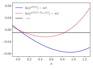
Figure 2: QoS control in finite time. $X(t)$ and $X_{\mathsf{n}+1}(t)$ are Poisson processes of duration $t$ with rates $\sum_{i=1}^{\mathsf{n}}\lambda_{i}=0.09$ and $\lambda_{\mathsf{n}+1}=0.05$. The QoS is set at $\gamma=-0.01$ , the capacity is $c=0.23$, and $t=1$. As there are values of $s$ such that the cumulant generating function of $X(t)+X_{\mathsf{n}+1}(t)$ is smaller than $sct-\gamma$, the condition (11) for $X(t)+X_{\mathsf{n}+1}(t)$ is satisfied and the new request $X_{\mathsf{n}+1}(t)$ can be accepted.

In short, we can now decide whether establishing a new connection can affect the promised QoS for a given time by computing the finite-time EB functions of the incoming traffic sources Kelly2014 . Clearly, finite-time EB functions can also be calculated for the net load and the available work. Considering the long-time limit of $\Lambda(s,t)$ leads to natural connections to statistical mechanics and to the cloning algorithm developed in that field, as discussed in the following subsections.

III.2 Asymptotic analysis

To study the long-time limit, we assume that the net-load process satisfies a large deviation principle, loosely written in the form

$$\mbox{\small Prob}\{W(t)=wt\}\asymp\mathrm{e}^{-t\hat{e}(w)}$$ (15)

with rate function $\hat{e}(w)$, where the symbol $\asymp$ means logarithmic equality in the limit as $t\to\infty$. The rate function $\hat{e}(w)$ encodes for the fluctuations around the typical value $\overline{w}$, which are of interest in resource allocation. As an aside, if $\hat{e}(w)$ is convex, then the large deviation principle (15) implies

$$\mbox{\small Prob}\{W(t)>wt\}\asymp\mathrm{e}^{-t\hat{e}(w)}$$ (16)

for $w>\overline{w}$, as the probability on the left-hand side is dominated by the slowest decaying contribution. The rate function can be obtained from the scaled cumulant generating function (SCGF)

$$e_{W}(s)=\lim_{t\to\infty}\frac{1}{t}\ln\langle\mathrm{e}^{sW(t)}\rangle,$$ (17)

when the latter is differentiable, by means of a Legendre–Fenchel (LF) transform

$$\hat{e}(w)=\sup_{s}\{sw-e_{W}(s)\}.$$ (18)

The inverse of equation (18) is also verified, i.e.,

$$e_{W}(s)=\sup_{w}\{sw-\hat{e}(w)\},$$ (19)

as reviewed in reference Touchette2009 .

More care is needed when the SCGF is non-differentiable. In fact, more generally, the LF transform of $e_{W}(s)$ yields the convex envelope of $\hat{e}(w)$ which can contain linear sections corresponding to the non-differentiable points of $e_{W}(s)$, interpreted as dynamical phase transitions Bertini2006 . In this paper, we will not deal with such circumstances.

Similarly to section III.1, we now turn our attention to the event that the service request overflows the capacity. Specifically, we require that the net load exceeds a specified $q>0$ at any finite time $\tau$ in $(0,t]$. To study this probability we can make the following heuristic argument based on the discrete-time analogue (see, e.g., references Lewis1996 ; Srikant2013 ).

First we note that to find the supremum of $W(\tau)$ it suffices to consider only the transition times $t_{i}$ and the final time $t$. Hence we have the inequality

$$\mbox{\small Prob}\left\{\sup_{0<\tau\leq t}\,W(\tau)>q\right\}\leq\sum_{n=1}^{\infty}\int_{0}^{t}\mathrm{d}t_{1}\int_{0}^{t}\mathrm{d}t_{2}\ldots\int_{0}^{t}\mathrm{d}t_{n}\,p(t_{1},t_{2},\ldots,t_{n})\sum_{i=1}^{n}\mbox{\small Prob}\{W(t_{i})>q\}+\mbox{\small Prob}\{W(t)>q\},$$ (20)

where $p(t_{1},t_{2},\ldots,t_{n})$ is the joint probability density to have transitions at times $t_{1},t_{2},\ldots,t_{n}$. We expect this inequality to become tighter for larger $q$ where the probability of exceedance at more than one time becomes small.

Now, since the net load typically decreases in time (becomes more negative) according to the stability condition of section II, the probability that $W(t)$ exceeds $q$ approaches zero as $t\to\infty$. Indeed we anticipate that the most likely time for exceedance scales with $q$. For large $q$ and $t$ this suggests using (16) to approximate $\mbox{\small Prob}\{W(t_{i})>q\}$ by $\mathrm{e}^{-q\frac{\hat{e}(q/t_{i})}{q/t_{i}}}$. The right-hand side of (20) is then dominated by the smallest exponent $\inf_{w\geq q/t}{\hat{e}(w)}/{w}$, where the condition $w\geq q/t$ follows from $t_{i}\leq t$. For $t\gg q$, this infimum occurs at a $t$-independent value $\arg\inf\hat{e}(w)/w=q/\tau^{*}$, consistent with our intuition that the most significant contribution to the probability (20) comes from a time which scales with $q$.

Putting everything together, we obtain

$$\mbox{\small Prob}\left\{\sup_{0<\tau\leq t}\,W(\tau)>q\right\}\asymp\mathrm{e}^{-q\delta},$$ (21)

which expresses an important asymptotic result for $t\to\infty$ and $q\to\infty$, with $q/t\to 0$. The exponent $\delta$ is the largest number $s$ such that $s-\hat{e}(w)/w\leq 0$ for all $w\geq 0$, or the largest number $s$ such that $e_{W}(s)$ is non-positive, using equation (19). Hence, the inequality

$$e_{W}(\delta)\leq 0$$ (22)

is satisfied.

It is worth noting that the same arguments can be applied to study the asymptotic probability that the queue occupation $Q(t)$ (rather than the net load) overflows $q$, which is obviously more interesting for applications. In fact, from equation (2), we get

$$\mbox{\small Prob}\left\{Q(t)>q\right\}=\mbox{\small Prob}\left\{\sup_{0<\tau\leq t}\int_{\tau}^{t}\mathrm{d}u\,\mathrm{w}(u)>q\right\},$$ (23)

which, by the same heuristic argument used to obtain equations (20) and (21), gives

$$\mbox{\small Prob}\left\{Q(t)>q\right\}\asymp\mathrm{e}^{-q\delta}.$$ (24)

As in section III.1, we focus on net loads of the form (3), whose exponent $\delta$ is given by

$$\delta(c)=\sup\{s:e_{X}(s)/s\leq c\},$$ (25)

with the assumption that the stability condition $\bar{x}<c$ is satisfied. The functional

$$\Lambda(s)=\frac{e_{X}(s)}{s}$$ (26)

represents the observable to be compared against the true capacity $c$ and is referred to as the asymptotic EB function or simply the EB function of the process $X(t)$. Note, we use the notation $\delta(c)$ in equation (25) and elsewhere when we wish to emphasize dependence of the exponent on $c$. The definition (26) holds for generic extensive processes. However, here we are chiefly interested in the case where $X(t)$ is the arrival process and cannot decrease in time. This implies that its rate function has non-negative support and the Legendre duality in turn implies that $\Lambda(s)$ is a monotonic non-decreasing function of $s$.

As we did with equation (14), we can assess the impact of an incoming service request on the available resources by computing the residual $\Lambda(s)-c$. The stability condition ensures that, on average, all the incoming requests are served, i.e., equation (11) is satisfied in the long-time limit for all real $\gamma$. On the other hand, it is of little practical interest to consider the case where $c$ is larger than the peak arrival rate, as this would ensure an excellent QoS for all times, but at the cost of having unused resources for most of the time. To find a more refined bound, let us request that the probability decays faster than a certain reference law, i.e.,

$$\mbox{\small Prob}\left\{\sup_{0<\tau\leq t}\,W(\tau)>q\right\}<\mathrm{e}^{-q\xi}.$$ (27)

The exponent $\xi$ is a way of defining a target asymptotic QoS, and, obviously, the larger its value the better service the final user is provided with. Using the asymptotic relation (21) yields $\delta(c)>\xi$, which implies

$$\Lambda(\delta(c))>\Lambda(\xi),$$ (28)

due to monotonicity. We also have that $c=\Lambda(\delta(c))$, i.e., $\Lambda$ and $\delta$ are inverse functions. This gives us the criterion

$$c>\Lambda(\xi)$$ (29)

to assess if the capacity $c$ is adequate to service the arrival process $X(t)$, given a target value of $\xi$.

It is worth noting that the notions that we have defined so far have glorious analogues in equilibrium statistical mechanics Reichl2009 , which we outline here without aiming at being exhaustive. In fact, equilibrium statistical mechanics is formulated in the limit of the size $\mathfrak{n}$ of a macroscopic system approaching infinity, under the assumption that the density $\Omega(\epsilon)$ of microscopic states having a mean energy $\epsilon$ satisfies

$$\Omega(\epsilon)\asymp\mathrm{e}^{\mathfrak{n}\mathrm{s}(\epsilon)};$$ (30)

the total energy $\mathfrak{n}\epsilon$, which is extensive in the size, has the same role as the net load, which is extensive in time, while $\mathrm{s}(\epsilon)$ is the micro-canonical entropy function of the system and is analogous to $\hat{e}_{W}(w)$. Another fundamental quantity in statistical mechanics is the Helmholtz free energy $\mathrm{A}(\beta)$, which is obtained from the entropy function via an LF transform, with variable $\beta$ conjugated to the mean energy $\epsilon$, followed by scaling by $\beta$. Here $\beta$ is the reciprocal $1/(k_{B}T)$ of the system temperature $T$ and $k_{B}$ is the Boltzmann constant. The function $\mathrm{A}(\beta)$ conveys the same information as the entropy $\mathrm{s}(\epsilon)$ (when that function is strictly concave and differentiable), but sometimes in thermodynamics it is more convenient to use the former than the latter. In fact, the Helmholtz free energy is analogous to the EB function $\Lambda(s)-c$ for a net load of the form (3), where the parameter $s$ is conjugated to the time-averaged load. Similarly to the thermodynamic analogues, the EB function follows from an LF transform and encodes for the same information as $\hat{e}(w)$, while its use is recommended over the rate function if one wants to assess to what extent the fluctuations affect the QoS. We can control the value of the conjugated variable $s$ by setting it to $\xi$, which represents the (rather arbitrary) target exponential tail of the probability in equation (27) and is positive. The EB $\Lambda(\xi)$ can be thought of as a macroscopic quantity, which describes the resource available to the user and can be derived from the microscopic dynamics of $X(t)$. Obviously, $\Lambda(\xi)$ is additive in the number of service requests as we can obtain the EB of pooled independent processes by summing the individual EBs of each process.

The focus on time-extensive observables $X(t)$, $Y(t)$, and $W(t)$ suggests even closer connections with non-equilibrium statistical mechanics, which essentially deals with time-extensive “currents” rather than with the size-extensive energy Zia2007 ; Derrida2007 ; Touchette2013 . As an aside, it is also worth noting that the asymptotic result (21) is reminiscent of recent results on the universal statistics of extrema for observables such as entropy Neri2017 ; see in particular Chetrite2018 for analysis of the housekeeping heat, which, similarly to the net load, is an observable that on average decreases with time. The analogies outlined in this paragraph suggest the exploitation of methods borrowed from non-equilibrium statistical mechanics, such as the so-called “cloning method” for the computation of $\Lambda(s)$. This is the topic of the next subsection.

III.3 Monte Carlo evaluation

Computing large deviation functionals by means of Monte Carlo methods is hard, as time-intensive observables are doomed to converge to their typical values. An approach that prevents such a fate from happening in simulations is the “cloning method” Anderson1975 ; DelMoral2004 ; Giardina2006 ; Giardina2011 . This enables a desired functional to be evaluated directly by propagating an ensemble of trajectories in time and cloning/pruning such trajectories appropriately. The cloning method has deep roots in mathematical physics Metropolis1949 ; Anderson1975 and can be thought of as a sequential Monte Carlo (SMC) strategy, also sometimes referred to as sequential importance resampling (SIR) Doucet2011 , tailored to sample large deviation events. While SMC is typically presented in a discrete-time setting (but see Fearnhead2017 for rigorous details on SMC in continuous time), the cloning method has been extensively used for continuous-time Markov processes, as proposed in Lecomte2007 . For the present EB formalism it is convenient to adapt the procedure of reference Cavallaro2016 , which also includes the case of non-Markovian continuous-time processes. Central to this procedure is to define and simulate the time $\tau$ between two consecutive random events occurring at $t_{n}$ and $t_{n+1}$ and the corresponding increment $\Theta_{n}$ in the value of the driven observable, as defined for $n=1,2,\ldots$ in section II; this can be easily done for both fluid and point processes. The aim is to estimate the SCGF as the exponential growth of $\langle\mathrm{e}^{sX(t)}\rangle$, which, loosely speaking, can be obtained from the ensemble of simulated trajectories if each is cloned (or pruned) when its configuration changes from $n$ to $n+1$ according to a factor $\mathrm{e}^{s\Theta_{n}}$, while the average cloning (or pruning) rate is monitored. More precisely, the algorithm consists of the following steps:

1. Set up an ensemble of $N$ clones, each with a time variable $t$, a random configuration $x_{0}$, and a counter $n=0$. Set a variable $C$ to zero. For each clone, simulate the time $\tau$ until the next event and set $t$ to $\tau$. Then, choose the clone with the smallest value of $t$.

2. For the chosen clone increase the observable by an amount $\Theta_{n}$ and update $n$ to $n+1$.

3. Increment the value of $t$ for the chosen clone to $t+\tau$, where $\tau$ is the waiting time for the clone until the next event, i.e., until $t_{n+1}$.

4. Compute $y=\lfloor\mathrm{e}^{s\Theta_{n}}+u\rfloor$, where $u$ is drawn from the uniform distribution on $[0,1)$.

   1. If $y=0$, prune the current clone. Then replace it with another one, uniformly chosen among the remaining $N-1$.

   2. If $y>0$, produce $y$ copies of the current clone. Then, prune a number $y$ of elements, uniformly chosen among the existing $N+y$.

5. Increment $C$ to $C+\ln[(N+\mathrm{e}^{s\Theta_{n}}-1)/N]$. Choose the clone with the smallest $t$, and repeat from 2) until $t$ for a chosen clone reaches the desired simulation time $T$.

The EB is finally recovered as $C/(sT)$ for large $T$. This prescription can suffer from finite-ensemble errors if any of the numbers $s\Theta_{n}$ is large enough for a single clone to replace a conspicuous fraction of the existing ensemble elements. Such an effect can be alleviated by choosing large $N$; for further discussion on this and related points, see Hurtado2009 ; Cavallaro2015 ; Nemoto2016 ; Brewer2018 ; Angeli2019 .

In the next sections we will consider selected Markovian and non-Markovian processes (fluid processes in section IV and point processes in sections V and VI) and demonstrate that the cloning method reproduces exact analytical solutions within numerical accuracy and thus can be reliably used as an automated way to compute the EB.

IV Markov fluid process

Introducing the EB in the previous section involved us defining a service that is provided at a constant deterministic rate $c$. This led to the notion of a fluid process, which describes the continuous flow in or out of a source (or server) subject to random periods of filling and emptying. The fluid process was arguably first introduced by P. A. P. Moran to describe the level of a dam, based on a discrete-time stochastic process Moran1954 . Since then, continuous-time variants have also been analysed, with remarkably many contributions to modelling of high-speed data-networks, building on reference Anick1982 . Although Markov fluids are well known to many specialists in traffic and queueing modelling Gautam2012 , it is worth dedicating a whole section to them, as they provide an elegant setting to demonstrate the EB and the cloning method.

We call an observable a Markov fluid if its time derivative is a function of a continuous-time Markov process. To illustrate this, we consider a server that can be in many states, and during the stay in each state releases a fluid with a certain deterministic rate. In such a model, deterministic and stochastic dynamics coexist, and the traffic generated can be thought of as a piece-wise continuous flow, in contrast with standard discrete-packet models. The flow intensity varies according to the state of an underlying continuous-time stochastic process with state space $\mathcal{S}$ and generator $\mathbf{G}$. Each state $i\in\mathcal{S}$ corresponds to a different flow intensity $b_{i}$. This generates a process which we refer to as $B(t)$ and can generically represent an arrival, a service or a net-load process.

As an example of an arrival process we can combine a number $\left|\mathcal{S}\right|$ of identical sources, which can be active or inactive. In this case the configuration state of the underlying Markov chain has dimension $\left|\mathcal{S}\right|$, each state corresponding to the number of active sources, with the total flow at its peak when all the sources are active Anick1982 .

For a general fluid, the rates $b_{i}$, $i=1,2,\ldots,\left|\mathcal{S}\right|$ are organised into the matrix $\mathbf{B}=\mathrm{diag}(b_{1},b_{2},\ldots,b_{\left|\mathcal{S}\right|})$. If the underlying Markov chain has transitions at times $t_{1},t_{2},\ldots,t_{n}$, with $0\leq t_{1}\leq t_{2}\leq\ldots\leq t_{n}\leq t$, the fluid process can be written as the continuous functional

$$B(t)=t_{1}b_{\mathsf{s}(0)}+\sum_{i=1}^{n-1}(t_{i+1}-t_{i})b_{\mathsf{s}(t_{i})}+(t-t_{n})b_{\mathsf{s}(t_{n})},$$ (31)

where $\mathsf{s}$ here simply maps the transition time to the underlying configuration immediately after it. We have chosen the symbol $B$ in allusion to the “type B” observables defined in non-equilibrium statistical physics Garrahan2009 ; Jack2015 . Similarly to such observables, each term of $B(t)$ only depends on the configuration immediately after $t_{i}$ and the time increment $t_{i+1}-t_{i}$ (except for the last term which only contributes until $t$).

We now define a joint configuration–flow space and denote the probability of having a configuration $i$, at time $t$, with a value $\mathsf{B}$ for the observable $B(t)$ as $P_{i}(\mathsf{B},t)$. This probability is propagated for a short time interval $\tau$, up to the first order in $\tau$, as

$$P_{i}(\mathsf{B},t+\tau)=\sum_{j\neq i}[\mathbf{G}]_{ij}\tau P_{j}(\mathsf{B},t)\\ +(1+[\mathbf{G}]_{ii}\tau)P_{i}(\mathsf{B}-b_{i}\tau,t),$$ (32)

which yields, in the limit as $\tau\to 0$, the master equation

$$\frac{\mathrm{d}}{\mathrm{d}t}P_{i}(\mathsf{B},t)=\sum_{j}[\mathbf{G}]_{ij}P_{j}(\mathsf{B},t)-b_{i}\frac{\partial}{\partial\mathsf{B}}P_{i}(\mathsf{B},t),$$ (33)

where $i,j=1,2,\ldots,\lvert\mathcal{S}\rvert$ are generic configurations of the underlying Markov process and $[\mathbf{G}]_{ij}$ is the generic entry of $\mathbf{G}$. In matrix form we get

$$\frac{\mathrm{d}}{\mathrm{d}t}|P(\mathsf{B},t)\rangle=\mathbf{G}|P(\mathsf{B},t)\rangle-\mathbf{B}\frac{\partial}{\partial\mathsf{B}}|P(\mathsf{B},t)\rangle,$$ (34)

where $|P(\mathsf{B},t)\rangle$ is the column vector with entries $P_{1}(\mathsf{B},t),P_{2}(\mathsf{B},t),\ldots,P_{\mathcal{S}}(\mathsf{B},t)$. In the limit as $t$ approaches infinity, the observable $B(t)/t$ concentrates around its typical value

$$\bar{b}=\langle 1|\mathbf{B}|P^{*}\rangle,$$ (35)

where $\langle 1\rvert$ is the row vector with all entries equal to one and $|P^{*}\rangle$ is the stationary distribution of the underlying Markov chain, i.e., the solution of $\mathbf{G}|P^{*}\rangle=0$.

Now, the full system can be diagonalised with respect to the subspace of the $\mathsf{B}$s by means of an integral transform, which yields the biased master equation

$$\frac{\mathrm{d}}{\mathrm{d}t}\tilde{P}_{i}(t)=\sum_{j}[\mathbf{G}]_{ij}\tilde{P}_{j}(t)+sb_{i}\tilde{P}_{i}(t),$$ (36)

where $\tilde{P}_{i}(t)=\int_{0}^{\infty}\mathrm{d}\mathsf{B}\,\mathrm{e}^{s\mathsf{B}}P_{i}(\mathsf{B},t)$ and we assume that the boundary conditions are such that $\mathrm{e}^{s\mathsf{B}}P_{i}(\mathsf{B},t)|_{0}^{\infty}=0$; more care is needed when these boundary conditions are not satisfied, but cloning simulations confirm that the approach works well in practice. Equation (36) corresponds to the dynamics of a system that changes configuration according to $\mathbf{G}$, whose weight evolves exponentially with rate $sb_{i}$ during the stay in state $i$, and feeds $B(t)$ an amount $b_{i}\tau$ after each visit to $i$ of duration $\tau$. In matrix form this is equivalent to

$$\frac{\mathrm{d}}{\mathrm{d}t}|\tilde{P}(t)\rangle=(\mathbf{G}+s\mathbf{B})|\tilde{P}(t)\rangle$$ (37)

and has formal solution

$$|\tilde{P}(t)\rangle=\exp\left[(\mathbf{G}+s\mathbf{B})t\right]|\tilde{P}(0)\rangle.$$ (38)

The finite-time EB of a Markov fluid can be expressed as follows. The aim is to find $\Lambda(s,t)=\ln\langle\mathrm{e}^{sB(t)}\rangle/(st)$, where the angled-bracket expectation value is obtained by averaging over both the configuration and flow space, i.e.,

$$\langle\mathrm{e}^{sB(t)}\rangle=\int\mathrm{d}\mathsf{B}\,\langle 1|\mathrm{e}^{s\mathsf{B}}|P(\mathsf{B},t)\rangle.$$ (39)

Integrating over $\mathsf{B}$ component-wise and using equation (38) gives the form

$$\Lambda(s,t)=\frac{1}{st}\ln\langle 1|\exp\left[(\mathbf{G}+s\mathbf{B})t\right]|\tilde{P}(0)\rangle,$$ (40)

which also shows that the EB can be obtained by propagating in time an initial state $|\tilde{P}(0)\rangle$.

As a simple example, we focus now on a source modulated by a telegraph process, i.e., a two-state ($1$ and $2$) continuous-time Markov process with generator

$$\mathbf{G}=\left(\begin{array}[]{cc}-\alpha&\beta\\ \alpha&-\beta\\ \end{array}\right),$$ (41)

where $\alpha$ and $\beta$ are transition rates. The service request is produced deterministically at rate $b_{1}$ or $b_{2}$, when the configuration is $1$ or $2$, respectively, while the typical behaviour is given by

$$\overline{b}=\frac{\beta b_{1}+\alpha b_{2}}{\alpha+\beta}.$$ (42)

The biased master equation explicitly reads

$$\frac{\mathrm{d}}{\mathrm{d}t}\left(\begin{array}[]{c}\tilde{P}_{1}(t)\\ \tilde{P}_{2}(t)\end{array}\right)=\left(\begin{array}[]{cc}-\alpha+b_{1}s&\beta\\ \alpha&-\beta+b_{2}s\\ \end{array}\right)\left(\begin{array}[]{c}\tilde{P}_{1}(t)\\ \tilde{P}_{2}(t)\end{array}\right).$$ (43)

Such a model can describe a source that is either in an idle state, i.e., transmitting only a few packets, or in a active state and transmitting at its peak rate. Further assuming that the observation starts in the stationary distribution

$$|P^{*}\rangle=\left(\begin{array}[]{c}\frac{\beta}{\beta+\alpha}\\ \frac{\alpha}{\beta+\alpha}\end{array}\right),$$ (44)

we can compute the finite-time EB function

$$\Lambda(s,t)=\frac{1}{st}\ln\langle 1|\exp\left[\left(\begin{array}[]{cc}-\alpha+b_{1}s&\beta\\ \alpha&-\beta+b_{2}s\\ \end{array}\right)t\right]\,|P^{*}\rangle.$$ (45)

We now turn to consider the asymptotic properties of a stable net load, fed by a telegraph-modulated fluid source and serviced by a channel of constant capacity $c$. Such a system is described by a master equation equivalent to equation (33), with the addition of a loss term $c\,\partial P_{i}(\mathsf{B},t)/\partial\mathsf{B}$, which in matrix form reads

$$\frac{\mathrm{d}}{\mathrm{d}t}|P(\mathsf{B},t)\rangle=\mathbf{G}|P(\mathsf{B},t)\rangle-(\mathbf{B}-c\mathds{1})\frac{\partial}{\partial\mathsf{B}}|P(\mathsf{B},t)\rangle.$$ (46)

The observable $B(t)$ now represents a net load of the form (3). Upon a bilateral integral transform, equation (46) can be written instead as

$$\frac{\mathrm{d}}{\mathrm{d}t}|\tilde{P}(t)\rangle=\left[\mathbf{G}+s(\mathbf{B}-c\mathds{1})\right]|\tilde{P}(t)\rangle,$$ (47)

where the entries of $|\tilde{P}(t)\rangle$ are $\tilde{P}_{i}(t)=\int_{-\infty}^{\infty}\mathrm{d}\mathsf{B}\,\mathrm{e}^{s\mathsf{B}}P_{i}(\mathsf{B},t)$ and we now assume that the boundary conditions are such that $\mathrm{e}^{s\mathsf{B}}P_{i}(\mathsf{B},t)|_{-\infty}^{\infty}=0$.

For the fluid modulated by a telegraph process it is straightforward to verify that the asymptotic EB function is given by

$$\Lambda(s)=-\frac{1}{2s}\Big{\{}\alpha+\beta-(b_{1}+b_{2})s\\ -\sqrt{[\alpha+\beta-(b_{1}+b_{2})s]^{2}-4[b_{1}b_{2}s^{2}-(b_{1}\beta+b_{2}\alpha)s]}\Big{\}},$$ (48)

which is the leading eigenvalue of the biased generator of equation (43), divided by $s$. In figure 3 it is shown that the result obtained using the cloning method of subsection III.3 is consistent with the exact analytic solution, except for well documented finite-ensemble errors Hurtado2009 ; Cavallaro2016 at large positive values of $s$.

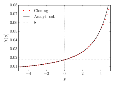
Figure 3: EB function for the telegraph fluid model with parameters $(\alpha,\beta,b_{1},b_{2})=(0.1,5,0,0.9)$. Markers correspond to cloning simulations with $(t,N)=(10^{4},10^{4})$, which underestimate the exact solution for large values of $s$ due to finite-ensemble effects (see main text).

Now, we are ready to tackle the problem of deciding whether, for this fluid traffic model, it is possible to guarantee a promised asymptotic QoS in the terms of inequality (27) with target $\xi$. The criterion (29) ensures that as long as the EB $\Lambda(\xi)$ is smaller than $c$, the user receives service as agreed with the provider.

V Markov modulated Poisson process

In this section, we consider sources modelled by Markov modulated Poisson processes (MMPPs), which can be thought of as the discrete counterparts of the fluid sources seen in the previous section, and, similarly to those, are ubiquitous in traffic and queueing modelling Fischer1993 ; Stewart2009probability ; Gautam2012 . As in fluid processes, in MMPPs, the load is modulated by the generator $\mathbf{G}$ and its intensity is defined by the diagonal matrix $\mathbf{B}=\mathrm{diag}(b_{1},\ldots,b_{\lvert\mathcal{S}\rvert})$. When the Markov chain is in state $i$, with $i=1,\ldots,\lvert\mathcal{S}\rvert$, events occur according to a pure birth process (Poisson process) with state space $\mathbb{N}^{0}$ and rate $b_{i}$. In fact, MMPPs and fluid processes share a number of additional features; for example, the parallelism between the concept of EB function for fluid processes and MMPPs is detailed in reference Elwalid1993 . Similarly to fluid processes, MMPPs have been extensively used for telecommunication modelling Fischer1993 (see also the application in appendix A) but have also been exploited for biological modelling Dobrzynski2009 ; Cavallaro2019 . A further interesting remark is that, even if MMPPs are modulated by a Markovian stochastic generator, the sequence of arrival events is non-Markovian, hence this framework can be used, in general, to model events that occur with time-varying rates Fischer1993 . If increments occur at times $t_{1},t_{2},\ldots,t_{n}$, the count process can be written as the functional

$$B(t)=\sum_{i=1}^{\infty}\mathbbm{1}_{t_{i}<t},$$ (49)

where $\mathbbm{1}_{x}$ is the indicator function of $x$.

The master equation for the joint MMPP and its underlying Markov process is

$$\frac{\mathrm{d}}{\mathrm{d}t}P_{i,\mathsf{B}}(t)=\sum_{j}[\mathbf{G}]_{ij}P_{j,\mathsf{B}}(t)+b_{i}P_{i,\mathsf{B}-1}(t)-b_{i}P_{i,\mathsf{B}}(t),$$ (50)

where $\mathsf{B}$ is the number of birth events which have occurred by time $t$ and $i,j=1,2,\ldots,\lvert\mathcal{S}\rvert$ are generic configurations of the modulating Markov process. A matrix representation akin to equation (46) is

$$\frac{\mathrm{d}}{\mathrm{d}t}|P(t)\rangle=\mathbf{G}\otimes\mathds{1}|P(t)\rangle+\mathbf{B}\otimes(a^{+}-\mathds{1})|P(t)\rangle,$$ (51)

where $|P(t)\rangle\in\mathcal{S}\otimes\mathbb{N}^{0}$ has elements $P_{i,\mathsf{B}}(t)$, while $a^{+}$ and $\mathds{1}$ are the creation and the identity operators, respectively, in $\mathbb{N}^{0}$. After a transform with $\tilde{P}_{i}(t)=\sum_{\mathsf{B}}\mathrm{e}^{s\mathsf{B}}P_{i,\mathsf{B}}(t)$ and suitable boundary conditions, equation (50) can be written as

$$\frac{\mathrm{d}}{\mathrm{d}t}\tilde{P}_{i}(t)=\sum_{j}[\mathbf{G}]_{ij}\tilde{P}_{j}(t)+b_{i}(\mathrm{e}^{s}-1)\tilde{P}_{i}(t).$$ (52)

In vector form we have

$$\frac{\mathrm{d}}{\mathrm{d}t}|\tilde{P}(t)\rangle=[\mathbf{G}+\mathbf{B}(\mathrm{e}^{s}-1)]|\tilde{P}(t)\rangle,$$ (53)

where $|\tilde{P}(t)\rangle$ has entries $\tilde{P}_{1}(t),\tilde{P}_{2}(t),\ldots,\tilde{P}_{n}(t)$. The finite-time EB function can be formally expressed as

$$\Lambda(s,t)=\frac{1}{st}\ln\langle 1|\exp\{[\mathbf{G}+(\mathrm{e}^{s}-1)\mathbf{B}]t\}|\tilde{P}(0)\rangle,$$ (54)

which is an analogue of equation (40). As a simple toy model, we consider the Poisson process modulated by the telegraph process with generator (41). Despite its simplicity, such a model captures the stochastic dynamics of gene expression when the gene is not self-regulated and switches between high and low activity phases, see, e.g., references Kepler2001 ; Horowitz2017 ; Tiberi2018 . Its EB function can be easily derived as

$$\Lambda(s)=-\frac{1}{2s}\Big{\{}\alpha+\beta-(b_{1}+b_{2})(\mathrm{e}^{s}-1)-\sqrt{[\alpha+\beta-(b_{1}+b_{2})(\mathrm{e}^{s}-1)]^{2}-4[b_{1}b_{2}(\mathrm{e}^{s}-1)^{2}-(b_{1}\beta+b_{2}\alpha)(\mathrm{e}^{s}-1)]}\Big{\}}.$$ (55)

The random variable $B(t)/t$ concentrates around the most probable value $\overline{b}$ given by equation (42). It is also worth noting the similarity in the form of equation (55) with the fluid EB function of equation (48); indeed the two expressions are the same to first-order approximation in $s$. In figure 4 the MMPP EB function (solid line in the figure) is shown to be accurately reproduced by cloning simulations (dot markers).

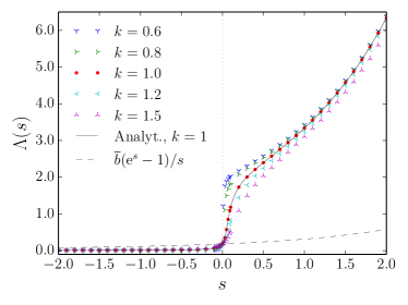
Figure 4: EB function for the two-state modulated Poisson process with $(b_{1},b_{2})=(0,2)$ and Weibull distributed switching times (56) and (57). Weibull distributions have rate parameters as defined in (58), with $(\alpha,\beta)=(0.01,0.1)$ and varying values of the shape parameter $k$. The case $k=1$ corresponds to an MMPP. Markers are results of cloning simulations with $(t,N)=(10^{4},10^{4})$. For comparison, the dashed line indicates the EB of a homogeneous Poisson process of rate $\bar{b}$.

As a remark, in the modulated Poisson processes, there are several net-load increments between two configuration changes, each increment being of unit magnitude. As a result, finite-ensemble effects are smaller than those of the fluid net load, where, in our simulations, increments are added only at configuration changes and depend exponentially on the inter-event time.

VI Non-Markov modulated Poisson process

Finally, and significantly, we introduce a generalization of the two-phase model described in section V by now considering that the arrival rate of the Poisson process is modulated by a semi-Markov process. Here the distributions of the lengths of the phases 1 and 2 are non-exponential thus exacerbating temporal correlations. Our choice is to draw the duration of phases 1 and 2 from the Weibull distributions

$$f_{1}(t|k,\tilde{\alpha}) =k\tilde{\alpha}^{k}t^{k-1}\mathrm{e}^{-(\tilde{\alpha}t)^{k}},$$ (56)

$$f_{2}(t|k,\tilde{\beta}) =k\tilde{\beta}^{k}t^{k-1}\mathrm{e}^{-(\tilde{\beta}t)^{k}},$$ (57)

with shape $k$ and rates $\tilde{\alpha}$ and $\tilde{\beta}$, respectively. The rate parameters are chosen to be

$$\tilde{\alpha}=\alpha\,\Gamma(1+1/k),\qquad\tilde{\beta}=\beta\,\Gamma(1+1/k),$$ (58)

where $\Gamma(x)$ is the Gamma function. This guarantees that each phase has the same mean duration as the process considered in the previous section and that the resulting modified arrival process converges to the same typical value (42); tuning the parameter $k$ only alters the fluctuation scenario.

Generally, for a non-Markov model such as the one described in this section, analytical progress is difficult; however, the cloning method remains a powerful way to evaluate the EB and thus assess the QoS numerically. This is illustrated in figure 4, where the EB functions for our semi-Markov modulated processes (non-dot markers in the figure) are compared to the standard MMPP case (which is obtained for $k=1$). The figure also shows the analytical result for a (homogeneous) Poisson process with identical value of $\overline{b}$, which clearly has very low effective bandwidth—adding a source of this type to the net load has little effect on the QoS.

On increasing the value of $k$ in the semi-Markov modulated process, the distributions of the durations become more peaked around their expected values, the traffic can be thought of as being more regular, and the effective bandwidth decreases (recall that $s>0$ is the relevant case here). Similarly, broad phase-length distributions (obtained by decreasing the value of $k$) correspond to strong fluctuations and high EB.

As a demonstration, we target an exponential decay with specific exponent $\xi$ for the net load and plot the EB $\Lambda(\xi)$ as function of $k$ in figure 5. For a given service capacity $c$, the statistics of the arrival requests can be modified by changing $k$ so that $\Lambda(\xi)<c$ (shaded area in figure 5) in order to provide the desired asymptotic QoS whilst maintaining the mean arrival rate (35). This type of modification is akin to the so-called “traffic shaping” MischaSchwartz1996 .

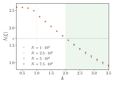
Figure 5: Cloning-simulation EB of semi-Markov modulated Poisson process with target exponent and bandwidth $(\xi,c)=(0.5,1.7)$. Parameters $\alpha,\beta,t$ are as in figure 4. Simulations with different values of $N$ are compared and suggest that finite-ensemble effects do not play a significant role, at least for $k<2$.

As alluded to above, having more regular on and off periods lowers the EB, thus leaving resources available for other requests but still maintaining the mean traffic $\bar{b}$. We see in figure 5 that, for $c=1.7$, this simple toy model achieves a target exponent of $\xi=0.5$ when $k$ exceeds a value around $2$. Arguably, similar considerations apply to more realistic models whose EBs can also be investigated by cloning; having a general numerical method to obtain $\Lambda(s)$ finally allows the use of criterion (29) to assess the asymptotic QoS.

VII Discussion

While physicists have been regarding the large deviation theory as an elegant way to formulate statistical mechanics, teletraffic engineers and operational researchers have been using large deviation results to estimate the likelihood that a demand in service overflows the available resources. A central role in teletraffic engineering is played by the effective bandwidth (EB) function $\Lambda(s)$. This function facilitates the construction of a neat criterion to decide whether a promised “quality of service” can be maintained in finite time and in the long-time limit, despite the threat of disruptive rare events. In this paper, we reviewed the concept of EB, showing that the function $\Lambda(s)$ can be thought of as a Helmholtz free energy and demonstrating that the cloning method, which has been developed in non-equilibrium statistical physics, is a general numerical scheme for the evaluation of $\Lambda(s)$.

The notion of EB is based on comparing the incoming requests (forming the packet traffic) with a very idealised protocol to process them, i.e., deterministic service of constant rate $c$. This is easily demonstrated in the Markov fluid process, for which analytical and numerical solutions are shown to be in excellent agreement. Nevertheless, non-Markovian systems are among those that can benefit the most from tools to predict the probability of large deviation events as has been discussed, e.g., in recent physics literature Andrieux2008 ; Maes2009 ; Cavallaro2015 ; Harris2015 ; Cavallaro2016 ; Sughiyama2018 . Hence, we focused on models from two classes of non-Markovian arrival processes (viz., the Markov and semi-Markov modulated Poisson processes) showing the extent to which the service-request statistics affect the EB. Simulation results on simple on-off toy models show that having more regular on and off periods lowers the EB, thus leaving resources available for other requests.

One can conceive further augmentation of the standard Markov modulated Poisson process (MMPP) by replacing, e.g., the modulated Poisson process with a generalised birth-death process. This generalization has been used to model populations in randomly switching environments modulated by a Markov generator (see, e.g., Hufton2016 and references therein). The lowest-order approximation of modulated birth-death processes leads to the piecewise-deterministic Markov processes (PDMPs) davis1984piecewise , which have also been recently shown to be appropriate for the natural sciences (where the underlying Markov process represents the extrinsic noise) Zeiser2010 ; Realpe-Gomez2013 ; Hufton2016 ; Lin2016 . Such PDMPs are reminiscent of the Markov fluid of section IV, but more general than that, as the deterministic evolution between jumps can be non-linear and the transition rate of the underlying process can depend on the fluid variable. We believe that the cloning method and the EB can contribute to straightforwardly exploring these more complex processes upon defining the correct cloning factor, with exponent given by an increment $\Theta_{n}$ which is non-linear in $\tau$. It is also worth mentioning that a non-equilibrium statistical mechanics of PDMPs has been presented in references Crivellari2010 ; Faggionato2009 .

Despite the fact that the specialised literature is rich in exact solutions (mainly for Markov processes, see, e.g., bucklew1990large ; shwartz1995large ; Weiss1995 ; Kelly1996 ; Lewis1996 and references therein), a systematic and general numerical scheme to compute the EB function $\Lambda(s)$ may be of practical interest. In this contribution we have argued that the cloning method of non-equilibrium statistical mechanics provides such a scheme and, significantly, can also be applied to non-Markovian processes. In fact realistic traffic models often incorporate memory as they convey the patterns of human dynamics, which are non-Markovian Huberman1997 ; Barabasi2005 . Hence, there is potentially much more that could be done in terms of actual applications, such as in the validation of traffic protocols and beyond.

Appendix A Statistics of packet loss

Let us consider modelling the occupation of a queue by a one-dimensional random walk on a linear chain of length $\mathsf{N}$. When the walker is in position $\mathsf{N}$, a new arrival (with rate $\lambda$) causes the total-current counter to tick, but leaving the occupation number (i.e., the underlying configuration $i$) unchanged. Such a system has a lucid interpretation in queuing theory and is referred to as an M/M/1/N queue in the so-called Kendall notation Stewart2009probability . Customers arrive according to a Poisson process at rate $\lambda$ and are processed by a single server at rate $\mu$, but there is space in the server for only $\mathsf{N}$ customers. When the server is fully occupied, there is no interruption of the arrival process; however the new customers do not alter the queue, simply disappearing instead. In communication systems, such customers are said to be “lost”. Formally, the occupation number of the queue follows a birth-death process, where the new arrivals can be neglected when $i\geq\mathsf{N}$. Hence, the stationary state has grand-canonical distribution

$$P^{*}_{i}=\frac{(1-\lambda/\mu)}{\left[1-(\lambda/\mu)^{\mathsf{N}+1}\right]}(\lambda/\mu)^{i},\quad i\leq\mathsf{N},$$ (59)

if $\lambda\neq\mu$, or $P^{*}_{i}=1/(\mathsf{N}+1)$, if $\lambda=\mu$, and satisfies the detailed-balance condition. Now suppose we are interested in the statistics of particle loss, i.e., we want to count the number of customers that arrive when the occupation number of the queue is $\mathsf{N}$. In the context of the present paper, we point out that this can be encoded into an MMPP with $[\mathbf{B}]_{ii}=0$, $i<\mathsf{N}$, and $[\mathbf{B}]_{\mathsf{N}\mathsf{N}}=\lambda$. The mean packet-loss rate is simply given by the arrival rate $\lambda$ times the probability $P^{*}_{\mathsf{N}}$ that the queue is full. Such arrivals correspond to jumps that leave that state as it is, but still contribute a factor $\mathrm{e}^{s}$ in the modified dynamics (defined in equation (53)). The MMPP framework thus provides one way to access fluctuations of the packet loss around its mean rate.

References

- [1] J. B. Anderson. A random-walk simulation of the Schrödinger equation: H+3. J. Chem. Phys., 63(4):1499, 1975.
- [2] D. Andrieux and P. Gaspard. The fluctuation theorem for currents in semi-Markov processes. J. Stat. Mech., 2008(11):P11007, 2008.
- [3] L. Angeli, S. Grosskinsky, and A. M. Johansen. Limit theorems for cloning algorithms, 2019. Preprint ariv:1902.00509.
- [4] D. Anick, D. Mitra, and M. M. Sondhi. Stochastic theory of a data-handling system with multiple sources. Bell Syst. Tech. J., 61(8):1871, 1982.
- [5] A. L. Barabasi. The origin of bursts and heavy tails in human dynamics. Nature, 435, 2005.
- [6] L. Bertini, A. De Sole, D. Gabrielli, G. Jona-Lasinio, and C. Landim. Non equilibrium current fluctuations in stochastic lattice gases. J. Stat. Phys., 123(2):237, 2006.
- [7] T. Brewer, S. R. Clark, R. Bradford, and R. L. Jack. Efficient characterisation of large deviations using population dynamics. J. Stat. Mech., 2018(5):053204, 2018.
- [8] J. A. Bucklew. Large Deviation Techniques in Decision, Simulation, and Estimation. Wiley, New York, NY, 1990.
- [9] M. Cavallaro and R. J. Harris. A framework for the direct evaluation of large deviations in non-Markovian processes. J. Phys. A Math. Theor., 49(47):47LT02, 2016.
- [10] M. Cavallaro, R. J. Mondragón, and R. J. Harris. Temporally correlated zero-range process with open boundaries: Steady state and fluctuations. Phys. Rev. E, 92(2):022137, 2015.
- [11] M. Cavallaro, M. D. Walsh, M. Jones, J. Teahan, S. Tiberi, B. Finkenstädt, and D. Hebenstreit. 3’–5’ crosstalk contributes to transcriptional bursting, 2019. Preprint bioRiv:10.1101/514174.
- [12] C.-S. Chang, P. Heidelberger, S. Juneja, and P. Shahabuddin. Effective bandwidth and fast simulation of ATM intree networks. Perform. Eval., 20(1):45, 1994.
- [13] V. Y. Chernyak, M. Chertkov, D. A. Goldberg, and K. Turitsyn. Non-equilibrium statistical physics of currents in queuing networks. J. Stat. Phys., 140(5):819, 2010.
- [14] R. Chétrite, S. Gupta, I. Neri, and É. Roldán. Martingale theory for housekeeping heat. Europhys. Lett., 124(6):60006, 2019.
- [15] M. R. Crivellari, A. Faggionato, and D. Gabrielli. Averaging and large deviation principles for fully-coupled piecewise deterministic Markov processes and applications to molecular motors. Markov Process. Relat., 16(3):497, 2010.
- [16] M. H. A. Davis. Piecewise-deterministic Markov processes: A general class of non-diffusion stochastic models. J. R. Stat. Soc. B, 46(3):353, 1984.
- [17] D. De Martino, L. Dall’Asta, G. Bianconi, and M. Marsili. A minimal model for congestion phenomena on complex networks. J. Stat. Mech., 2009(8):P08023, 2009.
- [18] D. De Martino, L. Dall’Asta, G. Bianconi, and M. Marsili. Congestion phenomena on complex networks. Phys. Rev. E, 79(1):015101, 2009.
- [19] P. Del Moral. Feynman-Kac Formulae: Genealogical and Interacting Particle Systems with Applications. Springer, New York, NY, 2004.
- [20] B. Derrida. Non-equilibrium steady states: fluctuations and large deviations of the density and of the current. J. Stat. Mech., 2007(7):P07023, 2007.
- [21] M. Dobrzynski and F. J. Bruggeman. Elongation dynamics shape bursty transcription and translation. Proc. Natl. Acad. Sci., 106(8):2583, 2009.
- [22] A. Doucet and A. M. Johansen. A tutorial on particle filtering and smoothing: Fifteen years later. In D. Crisan and B. Rozovskii, editors, The Oxford Handbook of Nonlinear Filtering, chapter 24, page 656. Oxford University Press, Oxford, 2011.
- [23] A. I. Elwalid and D. Mitra. Effective bandwidth of general Markovian traffic sources and admission control of high speed networks. IEEE/ACM Trans. Netw., 1(3):329, 1993.
- [24] A. Faggionato, D. Gabrielli, and M. R. Crivellari. Non-equilibrium thermodynamics of piecewise deterministic Markov processes. J. Stat. Phys., 137(2):259, 2009.
- [25] P. Fearnhead, K. Latuszynski, G. O. Roberts, and G. Sermaidis. Continuous-time Importance Sampling: Monte Carlo Methods which Avoid Time-discretisation Error, 2017. Preprint ariv:1712.06201.
- [26] W. Fischer and K. Meier-Hellstern. The Markov-modulated Poisson process (MMPP) cookbook. Perform. Eval., 18(2):149, 1993.
- [27] J. P. Garrahan, R. L. Jack, V. Lecomte, E. Pitard, K. van Duijvendijk, and F. van Wijland. First-order dynamical phase transition in models of glasses: an approach based on ensembles of histories. J. Phys. A Math. Theor., 42(7):75007, 2009.
- [28] N. Gautam. Analysis of queues: methods and applications. Taylor & Francis, London, 2012.
- [29] C. Giardinà, J. Kurchan, V. Lecomte, and J. Tailleur. Simulating rare events in dynamical processes. J. Stat. Phys., 145(4):787, 2011.
- [30] C. Giardinà, J. Kurchan, and L. Peliti. Direct evaluation of large-deviation functions. Phys. Rev. Lett., 96(12):120603, 2006.
- [31] R. J. Harris. Fluctuations in interacting particle systems with memory. J. Stat. Mech., 2015(7):P07021, 2015.
- [32] P. Heidelberger. Fast simulation of rare events in queueing and reliability models. ACM Trans. Model. Comput. Simul., 5(1):43, 1995.
- [33] J. M. Horowitz and R. V. Kulkarni. Stochastic gene expression conditioned on large deviations. Phys. Biol., 14(3):03LT01, 2017.
- [34] B. A. Huberman. Social dilemmas and internet congestion. Science, 277(5325):535, 1997.
- [35] P. G. Hufton, Y. T. Lin, T. Galla, and A. J. McKane. Intrinsic noise in systems with switching environments. Phys. Rev. E, 93(5):052119, 2016.
- [36] P. I. Hurtado and P. L. Garrido. Current fluctuations and statistics during a large deviation event in an exactly solvable transport model. J. Stat. Mech., 2009(02):P02032, 2009.
- [37] R. L. Jack and P. Sollich. Effective interactions and large deviations in stochastic processes. Eur. Phys. J. Spec. Top., 224(12):2351, 2015.
- [38] F. Kelly. Notes on effective bandwidths. In F. Kelly, S. Zachary, and I. Ziedins, editors, Stochastic Networks: Theory and Application, page 141. Oxford University Press, Oxford, 1996.
- [39] F. Kelly and E. Yudovina. Stochastic Networks. Cambridge University Press, Cambridge, 2014.
- [40] T. B. Kepler and T. C. Elston. Stochasticity in Transcriptional Regulation: Origins, Consequences, and Mathematical Representations. Biophys. J., 81(6):3116, 2001.
- [41] Christofer Larsson. Design of Modern Communication Networks. Elsevier, Amsterdam, 2014.
- [42] V. Lecomte and J. Tailleur. A numerical approach to large deviations in continuous time. J. Stat. Mech., 2007(3):P03004, 2007.
- [43] J. Lewis and R. Russel. An introduction to large deviations for teletraffic engineers (DIAS Technical Report), 1996.
- [44] Y. T. Lin and T. Galla. Bursting noise in gene expression dynamics: linking microscopic and mesoscopic models. J. R. Soc. Interface, 13(114):20150772, 2016.
- [45] C. Maes, K. Netočný, and B. Wynants. Dynamical fluctuations for semi-Markov processes. J. Phys. A Math. Theor., 42(36):365002, 2009.
- [46] N. Metropolis and S. Ulam. The Monte Carlo method. J. Am. Stat. Assoc., 44(247):335, 1949.
- [47] P. A. P. Moran. A probability theory of dams and storage systems. Aust. J. Appl. Sci., 5:116, 1954.
- [48] T. Nemoto, E. Guevara Hidalgo, and V. Lecomte. Finite-time and finite-size scalings in the evaluation of large-deviation functions: Analytical study using a birth-death process. Phys. Rev. E, 95(1):012102, 2017.
- [49] I. Neri, É. Roldán, and F. Jülicher. Statistics of Infima and Stopping Times of Entropy Production and Applications to Active Molecular Processes. Phys. Rev. X, 7(1):011019, 2017.
- [50] J. Realpe-Gomez, M. Baudena, T. Galla, A. J. McKane, and M. Rietkerk. Demographic noise and resilience in a semi-arid ecosystem model. Ecol. Complexity, 15:97–108, 2013.
- [51] L. E. Reichl. A Modern Course in Statistical Physics. Wiley, New York, NY, 2009.
- [52] D. Reijsbergen, P. T. De Boer, W. Scheinhardt, and B. Haverkort. Rare event simulation for highly dependable systems with fast repairs. Perform. Eval., 69(7-8):336, 2012.
- [53] M. Schwartz. Broadband Integrated Network. Prentice Hall, New York, NY, 1996.
- [54] A. Shwartz and A. Weiss. Large Deviations For Performance Analysis: Queues, Communication and Computing. Chapman & Hall, London, 1995.
- [55] R. Srikant and L. Ying. Communication Networks: An Optimization, Control and Stochastic Networks Perspective. Cambridge University Press, Cambridge, 2013.
- [56] W. J. Stewart. Probability, Markov Chains, Queues, and Simulation: The Mathematical Basis of Performance Modeling. Princeton University Press, Princenton, NJ, 2009.
- [57] Y. Sughiyama and T. J. Kobayashi. The explicit form of the rate function for semi-Markov processes and its contractions. J. Phys. A Math. Theor., 51(12):125001, 2018.
- [58] S. Tiberi, M. Walsh, M. Cavallaro, D. Hebenstreit, and B. Finkenstädt. Bayesian inference on stochastic gene transcription from flow cytometry data. Bioinformatics, 34(17):i647, 2018.
- [59] H. Touchette. The large deviation approach to statistical mechanics. Phys. Rep., 478(1-3):1, 2009.
- [60] H. Touchette and R. J. Harris. Large deviation approach to nonequilibrium systems, In R. Klages et al., editors, Nonequilibrium Statistical Physics of Small Systems: Fluctuation Relations and Beyond, page 335. Wiley, New York, NY, 2013.
- [61] A. Weiss. An introduction to large deviations for communication networks. IEEE J. Sel. Areas Commun., 13(6):938, 1995.
- [62] S. Zeiser, U. Franz, and V. Liebscher. Autocatalytic genetic networks modeled by piecewise-deterministic Markov processes. J. Math. Biol., 60(2):207, 2010.
- [63] R. K. P. Zia and B. Schmittmann. Probability currents as principal characteristics in the statistical mechanics of non-equilibrium steady states. J. Stat. Mech., 2007(07):P07012, 2007.