Bondi accretion for adiabatic flows onto a massive black hole with an accretion disk

In this paper, we present the classical Bondi accretion theory for the case of non-isothermal accretion processes onto a supermassive black hole (SMBH), including the effects of X-ray heating and the radiation force due to electron scattering and spectral lines.The radiation field is calculated by considering an optically thick, geometrically thin, standard accretion disk as the emitter of UV photons and a spherical central object as a source of X-ray emission. In the present analysis, the UV emission from the accretion disk is assumed to have an angular dependence, while the X-ray/central object radiation is assumed to be isotropic. This allows us to build streamlines in any angular direction we need to. The influence of both types of radiation is evaluated for different flux fractions of the X-ray and UV emissions with and without the effects of spectral line driving. We find that the radiation emitted near the SMBH interacts with the infalling matter and modifies the accretion dynamics. In the presence of line driving, a transition resembles from pure type 1 & 2 to type 5 solutions (see Fig 2.1, Frank et al. 2002), which takes place regardless of whether or not the UV emission dominates over the X-ray emission. We compute the radiative factors at which this transition occurs, and discard type 5 solution from all our models. Estimated values of the accretion radius and accretion rate in terms of the classical Bondi values are also given. The results are useful for the construction of proper initial conditions for time-dependent hydrodynamical simulations of accretion flows onto SMBH at the centre of galaxies.

1 Introduction

The spherically symmetric Bondi solution (Bondi 1952) has become a reference model for interpreting the observations of mass accretion onto supermassive black holes (SMBHs) in the centre of galaxies. This is so because SMBHs at the centre of elliptical galaxies are likely to accrete primarily from the surrounding hot, quasi-spherical interstellar medium, suggesting that accretion rates can be simply estimated using Bondi accretion theory. Studies on mass accretion were first considered in the framework of Newtonian gravity (Bondi & Hoyle 1944; Bondi 1952; Hoyle & Lyttleton 1939) and then they were generalized by Michel (1972) to curved spacetime. Quantum corrections to the general relativistic accretion have also been proposed (Yang 2015; Contreras et al. 2019). In recent years, the accretion onto SMBHs has been the subject of intense research because of its role in the co-evolution of SMBHs and their host galaxies. In particular, the number of these studies down to the parsec scale in the centre of galaxies has significantly increased with the advances in instrumental and computational capabilities (one example, is given by the Event Horizon Telescope Collaboration et al. 2019). On the other hand, fully analytical solutions on isothermal Bondi-like accretion including radiation pressure and the gravitational potential of the host galaxy have started to appear recently (Korol et al. 2016; Ciotti & Pellegrini 2017; Ciotti & Ziaee Lorzad 2018, hereafter KCP16, CP17 and CZ18). Moreover, recent detailed numerical calculations on Bondi accretion (Ramírez-Velasquez et al. 2018), using state-of-the-art consistent Smoothed Particle Hydrodynamics (SPH) techniques (Gabbasov et al. 2017; Sigalotti et al. 2018), suggest that it would be possible to push these studies further to cover the sub-parsec scales in active galactic nuclei (AGNs), including the effects of radiation pressure due to spectral lines (Ramírez-Velasquez et al. 2016, 2017).

Accretion onto compact objects is now recognized to be a major influencer on the environment surrounding SMBHs in the centre of galaxies (e.g., Salpeter 1964; Fabian 1999; Barai 2008; Germain et al. 2009). In the study of the several properties governing the evolution of the system, i.e., Bondi quantities such as the accretion rate and the solution of the hydrodynamical equations, a quite common assumption is to prescribe values of temperature, pressure and density at infinity and use them as the “true” boundary conditions for the solution of the equations, even when the problem at hand needs sub-parsec resolution scales as, for instance, in the case of AGNs. However, such resolution is never achieved in observational and numerical studies (Pellegrini 2005), introducing under- and over-estimations of the physical quantities (CP17). The outflow phenomenon is believed to play a major role in the feedback processes invoked by modern cosmological models (i.e., $\Lambda$-Cold Dark Matter) to explain the possible relationship between the SMBH and its host galaxy (e.g., Magorrian et al. 1998; Gebhardt et al. 2000) as well as in the self-regulating growth of the SMBH. The problem of accretion onto a SMBH has been studied via hydrodynamical simulations of galaxy evolution (e.g., Ciotti & Ostriker 2001; Di Matteo et al. 2005; Li et al. 2007; Ostriker et al. 2010; Novak et al. 2011). For example, in numerical studies of galaxy formation, spatial resolution permits resolving scales from the kpc to the pc, while the sub-parsec scales of the Bondi radius are not resolved. This is why a prescribed sub-grid physics is often employed to solve this lack of resolution. With sufficiently high X-ray luminosities, the falling material will have the correct opacity, developing outflows that originate at sub-parsec scales (e.g., Ramírez 2013). Therefore, calculations of the processes involving accretion onto SMBH have become of primary importance (e.g., Proga 2000; Proga et al. 2000; Proga 2003; Proga & Kallman 2004; Proga 2007; Ostriker et al. 2010). In order to provide a robust and reliable methodology for the production of initial conditions (ICs) for the numerical calculations of mass accretion onto SMBHs, we have combined the geometric effects and assumptions employed by Proga (2007) (hereafter P07) to compute the radiation field from the disk and central object with the analytical solution procedure provided by KCP16 and CP17.

In particular, P07 reported axisymmetric, time-dependent hydrodynamical calculations of gas flow under the influence of the gravity of black holes in quasars by taking into account X-ray heating and the radiation force due to electron scattering and spectral lines. He found that for a SMBH with a mass of $10^{8}M_{\odot}$ with an accretion luminosity of 0.6 times the Eddington luminosity, the flow settles into a steady state and has two components: an equatorial inflow and a bipolar inflow/outflow with the outflow leaving the system along the disk rotational axis and the inflow being a realization of a Bondi-like accretion flow. To calculate the radiation field an optically thin accretion disk was considered as a source of UV photons and a spherical central object as a source of X-rays. In contrast, KCP16 generalized the classical Bondi accretion theory, including the radiation pressure feedback due to electron scattering in the optically thin approximation and the effects of a general gravitational potential due to a host galaxy. In particular, they presented a full analytical discussion for the case of a Hernquist galaxy model. An extension of this analytical solution was reported by CP17 in terms of the Lambert-Euler $W$-function for isothermal accretion in Jaffe and Hernquist galaxies with a central SMBH. They found that the flow structure is sensitive to the shape of the mass profile of the host galaxy and that for the Jaffe and Hernquist galaxies the value of the critical accretion parameter can be calculated analytically.

In this paper we derive radiative, non-isothermal ($\gamma\neq 1$), angular-dependent streamline solutions for use as initial conditions in numerical simulations of mass accretion flows onto massive compact objects. To do so we introduce a radiation force term due to a non-isothermal extended source in the momentum equation as in P07 and develop a semi-analytical solution for the non-isothermal accretion onto a SMBH at the centre of galaxies using a procedure similar to that developed by KCP16 and CP17, with no assumption about the Bernoulli equation, but radially integrating the equations of motion. The effects of the gravitational potential due to the host galaxy are ignored here, and they will be left for a further analysis in this line. In Section 2, we introduce the mathematical methodology and the fundamental equations, while Section 3 contains the analysis of the results. Section 4 deals with the theoretical prediction of absorption lines. Section 5 deals with a general analysis of the bias in the estimates of the Bondi radius and mass accretion rate and discusses the importance of using the semi-analytical solution as true initial conditions for numerical simulations of accretion flows. Finally, Section 6 contains the relevant conclusions.

2 Bondi accretion for a non-isothermal flow

Under the assumption of spherical symmetry, the classical Bondi solution describes a purely adiabatic accretion flow on a point mass, for the case of a gas at rest at infinity and free of self-gravity. Detailed numerical calculations of the classical Bondi accretion flow onto a stationary SMBH were performed by Ramírez-Velasquez et al. (2018), using a mathematically consistent SPH method. In real situations, however, the accretion flow is affected by the emission of radiation near the SMBH. The radiation emitted near the SMBH interacts with the inflowing matter and modifies the accretion dynamics. The radiation effects can be strong enough to stop the accretion and shut off the central object. Here we follow the recipe of P07 to model the radiation field from the disk and central object, where a radiation force term is added as a source in the momentum equation. In this formulation, the disk is assumed to be flat, Keplerian, geometrically thin and optically thick. The structure and evolution of a flow irradiated by a central compact object can be described by the continuity and momentum equations

$$\frac{d\rho}{dt} = -\rho\nabla\cdot{\bf v},$$ (1)

$$\frac{d{\bf v}}{dt} = -\frac{1}{\rho}\nabla p+\boldsymbol{\mathrm{g}}+{\bf F}^{\rm rad},$$ (2)

where $\rho$ is the mass density, ${\bf v}=(v_{r},v_{\theta}=0,v_{\phi}=0)$ is the velocity vector, $p$ is the gas pressure, $\boldsymbol{\mathrm{g}}$ is the gravitational acceleration due to the central object, ${\bf F}^{\rm rad}=(F_{r},F_{\theta}=0,F_{\phi}=0)$ is the total radiation force per unit mass and $d/dt=\partial/\partial t+{\bf v}\cdot\nabla$. Under the assumption that $v_{\theta}=v_{\phi}=0$, Eq. (2) reduces to a single equation for the radial velocity component, which in spherical coordinates takes the form

$$\frac{\partial v_{r}(r,\theta,\phi)}{\partial t}+v_{r}(r,\theta,\phi)\frac{\partial v_{r}(r,\theta,\phi)}{\partial r} = -\frac{1}{\rho}\frac{\partial p(r,\theta,\phi)}{\partial r}$$ (3)

$$- \frac{\partial}{\partial r}\left(\frac{GM_{\rm BH}}{r}\right)$$

$$+ \frac{\partial}{\partial r}\left(\frac{C}{r}\right),$$

where $C$ is a constant whose value is given by the physical parameters of the system, while $\psi_{\rm grav}=(GM_{\rm BH})/r$ and $\psi_{\rm rad}=-C/r$, are the gravitational and radiation potentials, respectively. The opposite signs in the potentials indicate that the radiative and gravitational forces act in opposite directions. In the present analysis we will study the 1D problem, where $v_{r}(r,\theta,\phi)=v_{r}(r,\theta_{0})=v_{r}$, for a fixed angle $\theta_{0}$, and $p(r,\theta,\phi)=p(r,\theta_{0})=p$. With these assumptions Eq. (3) can be written in the more convenient form

$$\frac{\partial v_{r}}{\partial t}-p\frac{d}{dr}\left(\frac{1}{\rho}\right)+\frac{d\mathcal{H}(r)}{dr}=0,$$ (4)

where

$$\mathcal{H}(r)=\frac{p}{\rho}+\frac{1}{2}v_{r}^{2}-\psi_{\rm grav}-\psi_{\rm rad},$$ (5)

is the so-called Bernoulli function $\mathcal{H}(r)$, which will be used below to radially integrate equation (4). In equations (4) and (5), the gas pressure is related to the mass density by the equation

$$p=\frac{k_{B}\rho T}{\mu m_{p}}=p_{\infty}\tilde{\rho}^{\gamma},$$ (6)

where $k_{B}$ is the Boltzmann constant, $T$ is the gas temperature, $\mu$ is the mean molecular weight, $m_{p}$ is the proton mass, $1<\gamma\leq 5/3$ is the polytropic index and $\tilde{\rho}\equiv\rho/\rho_{\infty}$, where $p_{\infty}$ and $\rho_{\infty}$ are the values of the pressure and density at infinity, respectively. The polytropic sound speed is given by

$$c_{\rm s}^{2}=\frac{\gamma p}{\rho}.$$ (7)

The radiative acceleration on the right-hand side of equation (3) is composed of two parts: one due to electron scattering, which was first studied for the isothermal case by KCP16, CP17 and CZ18, and the other due to the radiation pressure produced by the spectral lines, which is here designed using the same strategy developed by P07. The disk luminosity $L_{\rm disk}$ and the central object luminosity $L_{\star}$ are expressed in terms of the total accretion luminosity $L$. That is, $L_{\rm disk}=f_{\rm disk}L$ and $L_{\star}=f_{\star}L=(1-f_{\rm disk})L$. As in P07, the disk is assumed to emit only in the UV (i.e., $f_{\rm disk}=f_{\rm UV}$), while the central object is assumed to emit only X-rays (i.e., $f_{\star}=f_{\rm X}$). In this way, the central object contributes to the radiation force due to electron scattering only, while the disk contributes to the radiation force due to both electron scattering and spectral lines. For simplicity, only the radiation force along the radial direction is considered, which for an optically thin gas is approximated by the relation

$$F_{r}^{\rm rad}(r)|_{\theta=\theta_{0}}=\frac{\sigma_{T}L}{4\pi r^{2}cm_{p}}\left[f_{\star}+2\cos\theta_{0}f_{\rm disk}(1+M(\tau))\right],$$ (8)

where $c$ is the speed of light, $\sigma_{T}/m_{p}$ is the mass scattering coefficient for free electrons, $\theta_{0}$ is some fixed and constant polar angle measured from the rotational axis of the disk, $\tau$ is the optical depth and $M(\tau)$ is the so-called force multiplier (Castor et al. 1975), which defines the numerical factor that parameterizes by how much spectral lines increase the scattering coefficient. According to P07, we use the following prescriptions for the force multiplier

$$M(\tau)=k\tau^{-\alpha}\left[\frac{(1+\tau_{\rm max})^{(1-\alpha)}-1}{\tau_{\rm max}^{(1-\alpha)}}\right],$$ (9)

where $k$ is a factor proportional to the total number of lines, $\alpha(=0.6)$ is the ratio of optically thick to optically thin lines, $\tau_{\rm max}=\tau\eta_{\rm max}$ and $\eta_{\rm max}$ is a parameter that determines the maximum value $M_{\rm max}=k(1-\alpha)\eta_{\rm max}^{\alpha}$. The parameters $k$ and $\eta_{\rm max}$ are given by the following relations (Stevens & Kallman 1990)

$$k=0.03+0.385\exp\left(-1.4\xi^{0.6}\right),$$ (10)

and

$$\ln\eta_{\rm max}=\cases{6}.9\exp\left(0.16\xi^{0.4}\right),&\quad{\rm if}\quad\ln\xi\leq 0.5,\\ 9.1\exp\left(-7.96\times 10^{-3}\xi\right),\quad{\rm if}\quad\ln\xi>0.5,{}$$ (11)

where $\xi$ is the photoionization parameter. As in P07, the photoionization parameter is calculated as $\xi=4\pi{\cal F}_{X}/n$, where ${\cal F}_{X}$ is the local X-ray flux and $n$ is the number density of the gas given by $n=\rho/(m_{p}\mu)$, with $\mu=1$. The local X-ray flux, corrected for the effects of optical depth, is defined by

$${\cal F}_{X}=\frac{L_{\star}}{4\pi r^{2}}\exp\left(-\tau_{X}\right),$$ (12)

where $\tau_{X}$ is the X-ray optical depth, which can be estimated by the integral

$$\tau_{X}=\int_{0}^{r}\kappa_{X}\rho dr,$$ (13)

between the central source ($r=0$) and a point $r$ in the accreting flow, where $\kappa_{X}$ is the absorption coefficient. Here the attenuation of the X-rays is calculated using $\kappa_{X}=0.4$ g^-1 cm² for all $\xi$.

Introducing the normalized quantities

$$x\equiv\frac{r}{r_{B}},\quad\tilde{c_{\rm s}}\equiv\frac{c_{\rm s}}{c_{\infty}}=\tilde{\rho}^{(\gamma-1)/2},\quad\mathcal{M}\equiv\frac{{v}_{r}}{c_{\rm s}},$$ (14)

where

$$r_{B}=\frac{GM_{\rm BH}}{c_{\infty}^{2}},$$ (15)

is the Bondi radius, $c_{\infty}^{2}=\gamma p_{\infty}/\rho_{\infty}$, $G$ is the Newtonian gravitational constant, $M_{\rm BH}$ is the mass of the black hole and $\mathcal{M}$ is the Mach number, and assuming a steady state motion (i.e., $\partial v_{r}/\partial t=0$), Eqs. (4) and (5) can be combined to give

$$\int\frac{d}{dr}\left(\frac{\mathcal{M}^{2}\tilde{c_{\rm s}}^{2}}{2}+\frac{\tilde{\rho}^{(\gamma-1)}}{\gamma-1}-\frac{1}{x}+\frac{l_{\rm tot}^{\rm rad}|_{\theta=\theta_{0}}}{x}\right)dr=0,$$ (16)

where $C|_{\theta=\theta_{0}}=GM_{\rm BH}l_{\rm tot}^{\rm rad}|_{\theta=\theta_{0}}$. The above integral is easily evaluated as follows

$$\int_{\mathcal{M}_{\infty}}^{\mathcal{M}}d\left(\frac{\mathcal{M}^{2}\tilde{c_{\rm s}}^{2}}{2}\right)=\frac{\mathcal{M}^{2}\tilde{c_{\rm s}}^{2}}{2}$$ (17)

$$\int_{\rho_{\infty}}^{\rho}d\left[\frac{\tilde{\rho}^{(\gamma-1)}}{\gamma-1}\right]=\frac{1}{\gamma-1}\left[\tilde{\rho}^{(\gamma-1)}-1\right]$$ (18)

$$\int_{r_{\infty}}^{r}d\left(-\frac{1}{x}+\frac{l_{\rm tot}^{\rm rad}|_{\theta=\theta_{0}}}{x}\right)=-\frac{1}{x}+\frac{l_{\rm tot}^{\rm rad}|_{\theta=\theta_{0}}}{x},$$ (19)

where $\mathcal{M}_{\infty}\to 0$ and $r_{\infty}\to\infty$. Integration of equation (16) leads to:

$$\tilde{\rho}^{(\gamma-1)}\left(\frac{\mathcal{M}^{2}}{2}+\frac{1}{\gamma-1}\right)=\frac{1}{x}-\frac{l_{\rm tot}^{\rm rad}|_{\theta=\theta_{0}}}{x}+\frac{1}{\gamma-1},$$ (20)

for the steady-state, radial, non-isothermal ($\gamma>1$), gravitational accretion, including the effects of radiation emission due to electron scattering and spectral discrete lines with appropriate boundary conditions at infinity, where

$$l_{\rm tot}^{\rm rad}|_{\theta=\theta_{0}}=l_{\rm Edd}^{\rm rad}f^{\rm rad}|_{\theta=\theta_{0}},$$ (21)

$l_{\rm Edd}^{\rm rad}=L/L_{\rm Edd}$, $L_{\rm Edd}=4\pi cGM_{\rm BH}m_{p}/\sigma_{T}$ is the Eddington luminosity, $\sigma_{T}=6.6524\times 10^{-25}$ cm² is the Thomson cross section and $f^{\rm rad}|_{\theta=\theta_{0}}$ is the radiative force parameter given by

$$f^{\rm rad}|_{\theta=\theta_{0}}=f_{\star}+2\cos\theta_{0}f_{\rm disk}[1+M(\tau)].$$ (22)

Although the force multiplier depends on the gas temperature through the parameter $k$, as shown by equation (17) of P07 based on detailed photoionization calculations performed with the XSTAR code (T. Kallman 2006, private communication), here we adopt the temperature-independent relation given by their equation (12) and leave the corrections for the temperature effects for future numerical work in this line (for instance, when using an energy equation accompanied by the net heating and cooling function developed by Ramírez-Velasquez et al. (2016, 2017).For example, see also Dannen et al. (2018).) The temperature correction for a fixed ionization parameter $\xi$ is explained in detail in P07, but here we provide a brief qualitative explanation. The dependence of the force multiplier on both $\xi$ and $T$ is an extremely complex problem, in part due to the amount and participation of the $\sim 10^{4}$ different atomic transitions given by neutral and ionized species from H to Fe. It is worth to explore in detail these relationships. However, we know that $r\sim 10$ pc is a good place to start such a study due to the amount of UV absorption transitions available for spectral line acceleration (Kashi et al. 2013; Higginbottom et al. 2014; Ramírez-Velasquez et al. 2016, 2017) and is suitable for the comparison we are proposing in this work. So we are computing the radiative factor for a $\xi_{\rm 10pc}=\xi(r={\rm 10\leavevmode\nobreak\ pc})$ without temperature corrections even though the hydrodynamical variables are taken to be temperature dependent. For instance, the dependence on temperature and ionization can be taken into account using the detailed Ramírez-Velasquez et al. (2017)’s Tables. Equation (20) must be solved coupled to the continuity equation (1), which in terms of the above assumptions and normalized parameters can be written as

$$x^{2}\mathcal{M}\tilde{\rho}^{(\gamma+1)/2}=\lambda,$$ (23)

where

$$\lambda=\frac{\dot{M}_{B}}{(4\pi f_{\rm solid})r_{B}^{2}\rho_{\infty}c_{\infty}},$$ (24)

is the dimensionless accretion parameter that determines the accretion rate for given $M_{\rm BH}$ and boundary conditions. In Eq. (24) $4\pi f_{\rm solid}=\int\sin\theta d\theta d\phi$ is the solid angle covered by the streamline at the polar angle $\theta_{0}$. When $f_{\rm solid}=1$ (full solid angle), we recover the classical accretion parameter. However, for the case of a $\theta_{0}$-dependent force $f_{\rm solid}<<1$. This dependence is important only for the final calculation of $\dot{M}_{B}=\lambda(4\pi f_{\rm solid})r_{B}^{2}\rho_{\infty}c_{\infty}$, which is fixed once the value of $\theta_{0}$ is chosen. Using Eq. (23) to eliminate $\tilde{\rho}$ from equation (20), the Bondi problem reduces to solving the equation:

$$g(\mathcal{M})=\Lambda f(x),\quad{\rm with}\quad\Lambda=\left[\chi_{\rm tot}^{\rm rad}|_{\theta=\theta_{0}}^{2}\lambda_{\rm cr}\right]^{2(1-\gamma)/(\gamma+1)},$$ (25)

where $\chi_{\rm tot}^{\rm rad}|_{\theta=\theta_{0}}=1-l_{\rm tot}^{\rm rad}|_{\theta=\theta_{0}}$, $\lambda$ is set equal to the critical value of the accretion parameter, defined as $\lambda=\chi_{\rm tot}^{\rm rad}|_{\theta=\theta_{0}}^{2}\lambda_{\rm cr}$, and

$$g(\mathcal{M}) = \mathcal{M}^{2(1-\gamma)/(\gamma+1)}\left(\frac{\mathcal{M}^{2}}{2}+\frac{1}{\gamma-1}\right),$$ (26)

$$f(x) = x^{4(\gamma-1)/(\gamma+1)}\left(\frac{\chi_{\rm tot}^{\rm rad}|_{\theta=\theta_{0}}}{x}+\frac{1}{\gamma-1}\right),$$ (27)

$$\lambda_{\rm cr} = \frac{1}{4}\left(\frac{2}{5-3\gamma}\right)^{(5-3\gamma)/[2(\gamma-1)]}.$$ (28)

Although equation (25) together with the definitions (26)-(28) look the same as those derived by KCP16 and CP17, there are some differences that are described in the following. On the other hand, it is clear from equation (25) that all physical quantities can be expressed in terms of the radial Mach number profile.

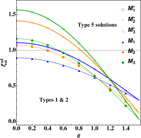
Figure 1: Angular dependence of the radiative force parameter for models $M_{1}$, $M_{2}$ and $M_{3}$ (when $M(\tau)=0$; thin dashed lines) and models $M_{1}^{\star}$, $M_{2}^{\star}$ and $M_{3}^{\star}$ (when $M(\tau)\neq 0$; thick lines). The horizontal line marks the value $l_{\rm tot}^{\rm rad}=1$. Just below this value, the matter will undergo a pure accretion process (type 1 solution), while above this value, it will suffer a transition to a type 5 outflow solution (which we discard). Each pair of models ($M_{i}$, $M_{i}^{\star}$) uses the same boundary conditions.

Compared to the previous analyses performed by KCP16 and CP17, the new feature of the present model is the angular dependence of the UV emission of the accretion disk, while it is assumed that the X-ray/central object radiation does not change with $\theta_{0}$. For an incident angle of $\theta_{0}=0$, the particles experience maximum intensity. As $\theta_{0}$ increases towards the equator, it follows from equation (22) that the radiation flux from the accretion disk becomes weaker until it vanishes for $\theta_{0}=\pi/2$. Consequently, the ratio between the X-ray and the UV flux increases with increasing $\theta_{0}$. Thus, for large $\theta_{0}$ pure gravitational accretion (type 1 solution) takes place until a critical angle $\theta^{\rm phase}$ develops for which radiation dominates over gravity and type 5 solutions result. In Fig. 1 we plot this feature of the solutions for three different flux fractions of the X-ray and UV emissions with and without the force multiplier. For instance, models $M_{1}$, $M_{2}$ and $M_{3}$ have $f_{\star}=0.5$ and $f_{\rm disk}=0.5$, $f_{\star}=0.2$ and $f_{\rm disk}=0.8$ and $f_{\star}=0.05$ and $f_{\rm disk}=0.95$, respectively, with $M(\tau)=0$ so that we can evaluate the influence of both types of radiation in detail. Models $M_{1}^{*}$, $M_{2}^{*}$ and $M_{3}^{*}$ are identical to models $M_{1}$, $M_{2}$ and $M_{3}$, respectively, but with $M(\tau)\neq 0$ and a radially varying ionization parameter given by

$$\xi=\frac{L}{n_{\rm H}r^{2}},$$ (29)

where the total accretion luminosity is set to be $L=7.45\times 10^{45}$ erg s^-1, which is appropriate for a SMBH of $10^{8}M_{\odot}$ at a distance $r=10$ pc, accreting at an efficiency of 8%. The gas density is $n_{\rm H}=10^{10}$ cm^-3 and the optical depth is set to $\tau=0.3$. The physical parameters employed for all these models are listed in Table 1. For all models we set $\theta_{0}=\theta_{\rm acc}^{\rm phase}$ and $\gamma=1.1$. The exploration of different values of the polytropic index $\gamma$ is a very complex topic. For instance, the “mirror” problem, Parker’s winds, with $3/2<\gamma<5/3$, and their spherical properties do change when angular momentum is added to the flow equations (Waters & Proga 2012). Also $\gamma=3/2$ is the critical adiabatic index that separates the solution space from their transonic behaviour. So, we plan to carefully look at $\gamma<3/2$ and $\gamma>3/2$ solutions, which lead to accelerating and decelerating Parker winds, respectively. The values of $f_{\star}$ and $f_{\rm disk}$ listed in Table 1 are the same employed by P07 and are guided by the observational results from Zheng et al. (1997) and Laor et al. (1997).

Table 1: Parameters of the generalized Bondi accretion models.

Run	Lines(a)	$f_{\rm\star}$	$f_{\rm disk}$	$\gamma$	$\theta^{\rm phase}$	$\theta^{\rm phase}_{\rm acc}$	$\theta^{\rm phase}_{\rm T5}$	$x_{\rm crit}$
					(rad)	(rad)	(rad)
M${}_{\rm 1}^{*}$	yes	0.50	0.50	1.1	$0.517465$	1.1	0.9	0.00856
M${}_{\rm 2}^{*}$	yes	0.20	0.80	1.1	$0.821151$	1.1	0.9	0.03350
M${}_{\rm 3}^{*}$	yes	0.05	0.95	1.1	$0.886684$	1.1	0.9	0.04559
M1	no	0.50	0.50	1.1	$na$	1.1	0.9	0.12149
M2	no	0.20	0.80	1.1	$0.391333$	1.1	0.9	0.00571
M3	no	0.05	0.95	1.1	$0.540618$	1.1	0.9	0.01332

(a) $M(\tau)\neq 0$ (yes) and $M(\tau)=0$ (no).

The angles $\theta^{\rm phase}_{\rm acc}$ and $\theta^{\rm phase}_{\rm T5}$ are given in terms of $\theta^{\rm phase}$, i.e., $\theta^{\rm phase}_{\rm acc}=1.1\theta^{\rm phase}$ and $\theta^{\rm phase}_{\rm T5}=0.9\theta^{\rm phase}$.

Models $M_{1}$, $M_{2}$ and $M_{3}$ represent non-isothermal accretion models with only the effect of electron scattering as in KCP16, CP17 and CZ18. A look to Fig. 1 shows that for model $M_{1}$, where the X-ray and UV emitters have each the same fraction of participation (50%) in the emission of radiation, there is no angle at which type 5 solutions are produced. In fact, model $M_{1}$ represents a pure accretion process with a nearly cancellation of the force of gravity close to $\theta_{0}=0$ and a radiative force parameter, $l_{\rm tot}^{\rm rad}|_{\theta=\theta_{0}}$, always below unity. In contrast, model $M_{1}^{*}$ with $M(\tau)\neq 0$ and $\theta^{\rm phase}\approx 0.51$ undergoes a transition from pure accretion to type 5 solution with $l_{\rm tot}^{\rm rad}|_{\theta=\theta_{0}}\approx 1.1$ at $\theta_{0}\approx 0$. Similarly, models $M_{2}$ and $M_{3}$ have values of $\theta^{\rm phase}$ for which there will be non physical solutions around $\approx 0.4-0.5$, while models $M_{2}^{*}$ and $M_{3}^{*}$ develop type 5 solutions for values of $\approx 0.82-0.90$. In what follows we shall explore in more detail these numerical solutions separately.

3 Analysis of the results

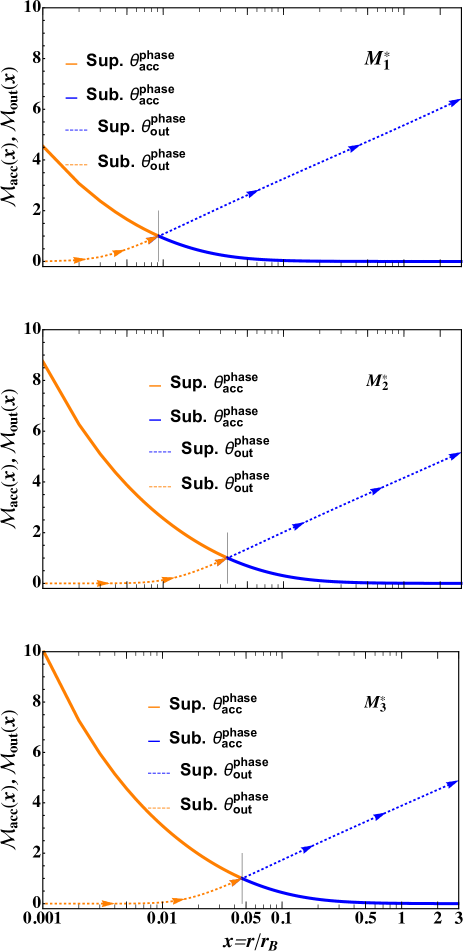
Figure 2: Mach number of the inflow (solid lines) and outflow (dotted lines) solutions of equation (20) with $M(\tau)\neq 0$. The supersonic part of the inflow solutions are depicted in orange, while the subsonic part is given in blue. In contrast, the supersonic outflow solution is depicted in blue and the subsonic one in orange. The vertical lines in each frame mark the position of the sonic radius. When the radiation dominates, the gas will escape from the gravitational potential of the accretor. The upper, middle and bottom frames correspond to models with $f_{\rm disk}=0.5,0.8$ and 0.95, respectively (see Table 1).

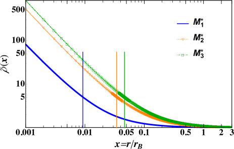
Figure 3: Density profiles of the radiative non-isothermal models with $M(\tau)\neq 0$. The vertical lines mark the position of the sonic radius for each model. As the UV emission becomes stronger, the accreting gas becomes supersonic at larger radial distances from the SMBH, while the density becomes higher for $x\lesssim 0.5$.

Figure 2 shows the radial Mach number profiles of the inflow (solid lines) and type 2 (dotted lines) solutions (which we are including into the discussion and which we will call outflow from now on) of equation (25) for models $M_{1}^{*}$, $M_{2}^{*}$ and $M_{3}^{*}$. The supersonic inflow ($\mathcal{M}>1$) solution is depicted in orange, while the subsonic ($\mathcal{M}<1$) solution is given by the blue lines. For model $M_{1}^{*}$, X-ray heating is the strongest (i.e., $f_{\star}=f_{\rm disk}=0.5$). In this case, the solution predicts a transition from pure accretion (i.e., $\theta_{0}>\theta^{\rm phase}$) to a type 5 flow with a critical radius $x_{\rm crit}\approx 0.0090$, where the supersonic and subsonic flows match to produce a full transonic flow. For model $M_{2}^{*}$, X-ray heating by the central object ($f_{\star}=0.2$) is smaller than the UV emission from the accretion disk ($f_{\rm disk}=0.8$) and we observe two important differences compared to model $M_{1}^{*}$. First, the critical point occurs at a larger radius ($x_{\rm crit}\approx 0.034$) and so the flow becomes supersonic at a distance from the SMBH about 4 times larger than for model $M_{1}^{*}$. Second, at an inner radius of $\approx 0.001$, the inflow for model $M_{2}^{*}$ reaches $\mathcal{M}\approx 8.1$ against $\approx 4.1$ for model $M_{1}^{*}$.

In Fig. 2, the supersonic outflow solution (type 2) is depicted by the dotted blue lines, while the subsonic solutions are given by the dotted orange lines. Notice that for the $M_{2}^{*}$ model, the winds are developed farther away from the centre, i.e., around $x\approx 0.034$ compared to model $M_{1}^{*}$, where the thermal outflows are produced closer to the central object at $x\approx 0.01$. Therefore, at larger distances from the SMBH, i.e., at $x\approx 3$, faster winds are developed for model $M_{1}^{*}$ ($\mathcal{M}(x=3)\approx 6.2$) compared to model $M_{2}^{*}$ for which $\mathcal{M}(x=3)\approx 4.4$. In all plots, the flows escaping supersonically from the gravitational potential of the SMBH are indicated by the arrows. When only 5% of the heating from the central object contributes to the radiation factor, as in model $M_{3}^{*}$, $x_{\rm crit}\approx 0.046$ and mass accretion proceeds supersonically below this radius with $\mathcal{M}\approx 10$ at $x=0.001$, while supersonic outflows are produced for $x\gtrsim 0.046$. The numerical simulations of P07 for $f_{\star}=f_{\rm disk}=0.5$ (his run case A) shows that a strong X-ray heating can accelerate the outflow to maximum velocities of 700 km s^-1 with the outflow collimation by the infall increasing with increasing radius. When $f_{\star}=0.2$ and $f_{\rm disk}=0.8$, line driving is seen to accelerate the outflow to higher velocities (up to 4000 km s^-1), while the outflow collimation becomes very strong for $f_{\star}=0.05$ and $f_{\rm disk}=0.95$, i.e., when the X-ray heating is the smallest, which corresponds to our model $M_{3}^{*}$. In this case, the gas outflow is confined within a very narrow channel along the equatorial axis of the accretion disk, while most of the computational volume is occupied by the inflow.

The density profiles for models $M_{1}^{*}$, $M_{2}^{*}$ and $M_{3}^{*}$ are shown in Fig. 3. As the UV emission intensity from the accretion disk becomes stronger, the gas density close to the SMBH becomes higher. This is counter-intuitive because we would have expected the radiation to push the gas away from the centre, resulting in decreasing density close to the SMBH. This is in fact the case. As the radiation intensity increases, it pushes the critical radius farther away from the SMBH and consequently the gas becomes supersonic at larger radial distances. As the supersonic flow occupies a larger central volume, the density close to the SMBH increases by factors as large as $\approx 10$ when going from $f_{\rm disk}=0.5$ to $f_{\rm disk}=0.95$.

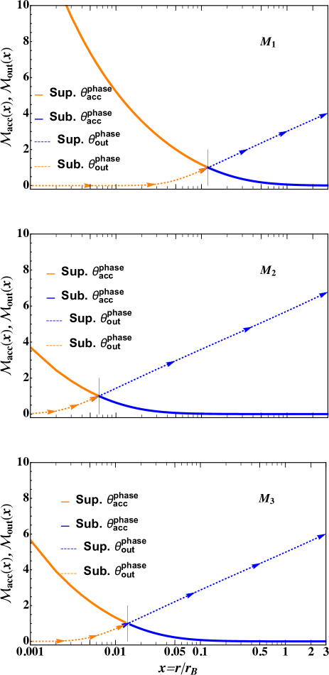
Figure 4: Mach number of the inflow (solid lines) and outflow (dotted lines) solutions of equation (20) with $M(\tau)=0$. The supersonic part of the inflow solutions are depicted in orange, while the subsonic part is given in blue. In contrast, the supersonic outflow solution is depicted in blue and the subsonic one in orange. The vertical lines in each frame mark the position of the sonic radius. When the radiation dominates, the gas will escape from the gravitational potential of the accretor. With no force multiplier, no winds are developed for $f_{\star}=f_{\rm disk}=0.5$ (model $M_{1}$).

The Mach number profiles for models $M_{1}$, $M_{2}$ and $M_{3}$ with no force multiplier are shown in Fig. 4. In the absence of line driving and strong X-ray heating (model $M_{1}$), no type 5 flows are developed regardless of the angle of incidence. In this case, the critical point occurs at $x\approx 0.12$ and close to the SMBH at $x=0.001$ the Mach number reaches values as high as $\approx 250$. As the UV emission intensity increases over the X-ray intensity (models $M_{2}$ and $M_{3}$), the critical point and the outflows occur at smaller radii from the SMBH compared to models $M_{2}^{*}$ and $M_{3}^{*}$. On the other hand, at radii sufficiently far from the SMBH, i.e., at $x=3$ the outflows become more supersonic than for models $M_{2}^{*}$ and $M_{3}^{*}$ as we may see by comparing Figs. 2 and 4. These results clearly show that radial velocities can differ from system to system depending on the details of the radiative processes dominating the source.

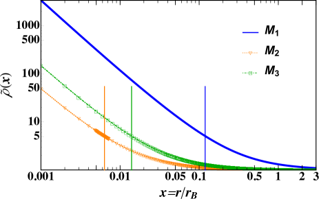
Figure 5: Density profiles of the radiative non-isothermal models with $M(\tau)=0$. The vertical lines mark the position of the sonic radius for each model. As the UV emission becomes stronger, the accreting gas becomes supersonic at larger radial distances from the SMBH, while the density becomes higher for $x\lesssim 0.2$. Note that these trends apply only to models $M_{2}$ and $M_{3}$, while model $M_{1}$, having an arbitrary $\theta_{0}$ and weaker UV emission, becomes supersonic at a much larger distance from the SMBH and achieves much higher central densities than models $M_{2}$ and $M_{3}$.

For our choice of $\theta_{0}=\theta_{\rm acc}^{\rm phase}$, Fig. 5 shows the density profiles for models $M_{1}$, $M_{2}$ and $M_{3}$. We see that model $M_{1}$ reaches a density as high as $\approx 3000$ at $x=0.001$, which is about 30 times larger than for model $M_{1}^{*}$. This result implies that when X-ray emission is strong enough, the accretion rate will also increase by the same factor and the accretion lifetime will decrease for systems with the same gas reservoirs. In contrast, as the UV emission intensity dominates over the X-ray emission, the effects of line driving are those of increasing the density close to the SMBH. In particular, comparing Figs. 3 and 5 we may see that the density at $x=0.001$ is from 10 to 5 times higher for models $M_{2}^{*}$ and $M_{3}^{*}$ than for models $M_{2}$ and $M_{3}$.

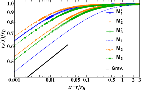
Figure 6: Estimated Bondi radius for all models. Models with $M(\tau)\neq 0$ are represented by the solid lines, while models with $M(\tau)=0$ are depicted by the dashed lines. For comparison, the black solid line displays the asymptotic behaviour for the pure gravitational case. In the limit when $x\to\infty$, $r_{e}\to r_{B}$.

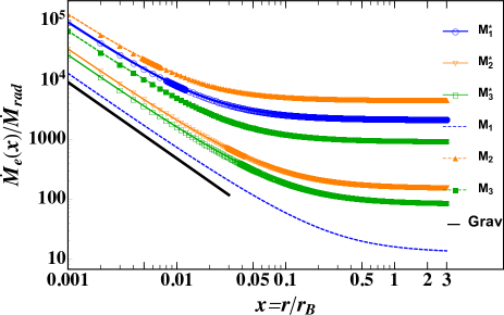
Figure 7: Estimated accretion rate for all models. Models with $M(\tau)\neq 0$ are represented by the solid lines, while models with $M(\tau)=0$ are depicted by the dashed lines. For comparison, the black solid line displays the asymptotic behaviour for the pure gravitational case.

4 Predicted pure absorption spectral line shape

A very important prediction of these models is the symmetry in shape of absorption spectral lines as seen by an observer far away from the system. To see that we imagine an atom falling onto the black hole as predicted by model $M^{*}_{1}$. That atom has a hypothetical transition which would absorb photons emitted by the inner region at 10 $\AA$ in the rest-frame ($\lambda_{0}$). Then we use the Doppler-shift formula (Rybicki & Lightman 1979):

$$w=\frac{w_{0}}{\gamma L(1-{\rm v}(x)\cos\phi/c)},$$ (30)

where $w$ is the angular frequency (measured by the observer) of an emitted photon with rest-frame frequency $w_{0}$. As it is used, $\gamma L$ is the Lorentz factor, ${\rm v}(x)$ is the velocity of the absorbing atom and $\phi$ is the angle between the streamline and the line-of-sight towards the observer, which we have set to $\phi=0$. For falling particles we use ${\rm v}(x)=-\mathcal{M}(x)c_{s}$, where $c_{s}$ is given by equation (7) , for a value of $\approx 345$ km s^-1. The simplest absorption model we could assume for the description of the absorption spectrum is

$$F_{\lambda}(x)=\exp\left[-A(x)\exp\left(-\frac{(\lambda(x)-\lambda_{0})^{2}}{\sigma^{2}}\right)\right],$$ (31)

where $\nu_{0}\lambda_{0}=(w_{0}/2\pi)\lambda_{0}=c$ and $\sigma$ is a representative width given by $0.1\%\lambda(x)$. We set $A(x)=\rho(x)/\rho_{\rm max}$ to model the intensity of the absorption taken from the density profile of each model, $\rho(x)=\tilde{\rho}(x)\rho_{\infty}$ and $\rho_{\rm max}=\tilde{\rho}(x=0.001)\rho_{\infty}$. As the particle is getting closer to the BH, the density is increasing and the final shape will tend to have a deeper deep shifted towards the red. From Figure 8, it is clear that the most asymmetrical line is the one with $f_{\star}=0.05$ (bottom panel, solid red line), for which the high-energy radiation is weaker leaving the particle to reach larger velocities and more asymmetry. On the other hand, we do not discuss the outflow (type 2 solution) profile, because the boundary conditions are not located at the base of the wind as we mentioned earlier. A deep discussion into the matter of asymmetrical absorption line shape is beyond the scope of the present work. An observational treatment in the Seyfert galaxy NGC 3783 can be found in (Ramírez et al. 2005). We leave the detailed description of infalling and outflowing real atoms and ionized species, like O vii, O viii, Fe xxv for future work, which are of extreme importance for our understanding of BH science.

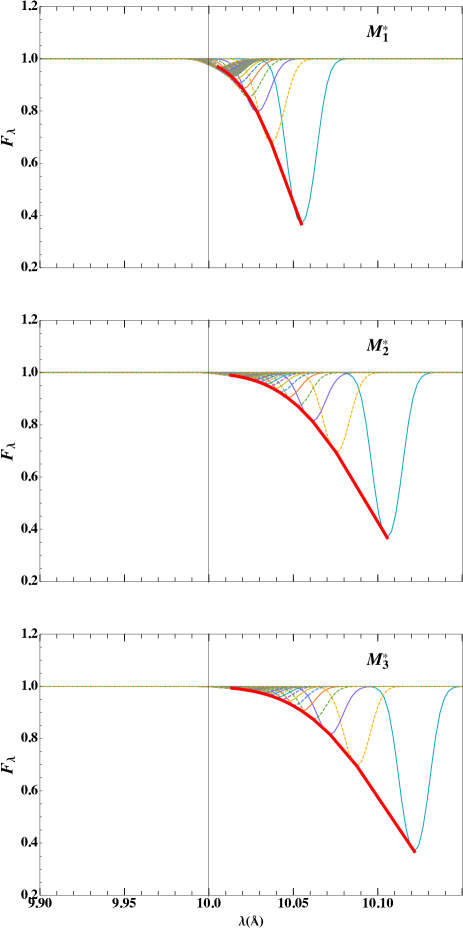
Figure 8: Predicted accretion absorption line shape for models $M_{1}^{*}$, $M_{2}^{*}$ and $M_{3}^{*}$. In each case, the solid red line shows the profile of a typical absorption line for an atom falling onto the BH.

5 Estimated Bondi radius and mass accretion applications

An important application of the present analysis is to quantify the differences between the true ($r_{B}$) and estimated ($r_{e}$) Bondi radius as well as the true ($\dot{M}_{\rm rad}$) and estimated ($\dot{M}_{e}$) accretion rate when the instrumental resolution is limited or the numerical resolution is inadequate at the sub-parsec scales. Following KCP16 and CP17, these differences as a function of radial distance from the central source are defined by the relations

$$\frac{r_{e;\{{\rm acc},{\rm out}\}}(x)}{r_{B}}=\left(\frac{x^{2}\mathcal{M}_{\{{\rm acc},{\rm out}\}}}{\chi_{\rm tot}^{\rm rad}|_{\theta=\theta_{0}}^{2}\lambda_{\rm cr}}\right)^{2(\gamma-1)/(\gamma+1)},$$ (32)

for the radius and

$$\frac{\dot{M}_{e;\{{\rm acc},{\rm out}\}}(x)}{\dot{M}_{\rm rad}}=\frac{1}{\chi_{\rm tot}^{\rm rad}|_{\theta=\theta_{0}}^{2}}\left[\frac{r_{e;\{{\rm acc},{\rm out}\}}(x)}{r_{B}}\right]^{-(5-3\gamma)/[2(\gamma-1)]},$$ (33)

for the accretion rate, where $\chi_{\rm tot}^{\rm rad}(\theta)$ is the angular-dependent radiative factor used in this work. In Fig. 6 we show the estimated values of the Bondi radius for all models. For comparison the solid black line is the estimated Bondi radius for the classical Bondi accretion problem. At small radii, i.e., at $x=0.001$, model $M_{1}^{*}$ has an estimated Bondi radius which is $\approx 0.64r_{B}$ compared to model $M_{3}^{*}$, which has $r_{e}/r_{B}\approx 0.51$ when the UV emission from the accretion disk dominates the radiation field. These values are comparatively lower than those resulting for models $M_{2}$ and $M_{3}$ with no spectral line driving, which have $r_{e}/r_{B}\approx 0.68$ and $\approx 0.6$, respectively. Moreover, comparing the asymptotic behaviour of $r_{e}/r_{B}$ for the pure gravitational case (solid black line) given by $r_{e}(x)/r_{B}\sim x^{3(\gamma-1)/2}$ when $x\to 0^{+}$ (see equation (22) of KCP16), we find differences of $\approx 10\%-40\%$ between the classical and present generalized Bondi models. In addition, for models $M_{1}$, $M_{2}$ and $M_{1}^{*}$ the ratio $r_{e}/r_{B}\to 1$ at $x\approx 0.1$, while at larger radii all models have values of $r_{e}/r_{B}$ close to unity, as shown in Fig. 6 for $x=3$.

The estimated accretion rates for all models are displayed in Fig. 7 as compared with the asymptotic behaviour of the pure gravitational accretion at small radii given by $\dot{M}_{e}(x)/\dot{M}_{B}\sim x^{-3(5-3\gamma)/4}$ (see equation (23) of KCP16). We may see that the radiative effects lead to an overestimation of the accretion rates. In particular at $x=0.001$, models $M_{1}$ and $M_{2}$ with $M(\tau)=0$ have accretion rates that are from 2 to 5 times larger than models $M_{1}^{*}$ and $M_{2}^{*}$. The differences between these models grow up to a factor of 10 at $x\approx 3$. The level of overestimation of the accretion rates compared to the classical Bondi problem is smaller when the effects of line driving are ignored (in $M_{1}$).

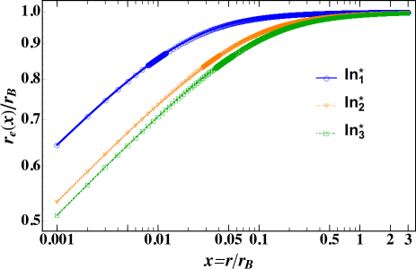
Figure 9: Estimated Bondi radius for all models with $M(\tau)\neq 0$. The solid line is for the $M_{1}^{*}$, dotted line is for the $M_{2}^{*}$, and dotdashed line is for the $M_{3}^{*}$ infalling material.

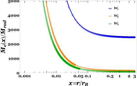
Figure 10: Estimated accretion rate for all models with $M(\tau)\neq 0$. The solid line is for the $M_{1}^{*}$, dotted line is for the $M_{2}^{*}$, and dotdashed line is for the $M_{3}^{*}$ infalling material.

Figure 9 shows the estimated values of the Bondi radius for models $M_{1}^{*}$, $M_{2}^{*}$ and $M_{3}^{*}$ for the inflow solutions (alone). For the type 5 solutions the limit of $r_{e}/r_{B}$ when $x\to\infty$ is no longer one, but deviates from it by about 10%. This occurs because $r_{B}$ looses its meaning for $\chi_{\rm tot}^{\rm rad}|_{\theta=\theta_{0}}\leq 0$, which is precisely the case here. For completeness, Fig. 10 displays the accretion rates as a function of the radial distance from the SMBH (with y-linear scale). The accretion rates associated with the type 5 flows are close to those associated with the infalling material with the differences not being larger than about 3%.

A further important application of these semi-analytical models is the construction of proper initial conditions for studying the stability of the Bondi accretion flow (Foglizzo et al. 2005). In most simulations of accretion flows the accretor is assumed to be stationary and small-scale density and velocity gradients that develop near it, which are the result of non-linear amplification of numerical noise, may lead to different flow patterns as the resolution is increased. This noise arises because mutually repulsive pressure forces do not cancel in all directions simultaneously, giving rise to non-radial velocities whose magnitudes are larger near the accretor. On the other hand, the use of standard artificial viscosity with a constant coefficient leads to spurious angular momentum advection in the presence of vorticity. However, the intrinsic noise generated due to numerical effects is not sufficient to make the flow unstable at parsec scales, while it may become prominent in the proximity of the accretor at sub-parsec scales. On the other hand, the strength and type of the instability may also depend on the size of the accretor (Blondin & Raymer 2012), the Mach number and the polytropic index $\gamma$. Understanding how these parameters can influence noise amplification at sub-parsec scales will shed light on the instability production mechanisms and the accretion rate for long-stage accretion systems.

6 Summary and conclusions

We have presented the classical Bondi accretion theory for the case of non-isothermal accretion processes onto a supermassive black hole (SMBH), including the effects of X-ray heating and the radiation force due to electron scattering and spectral lines. The radiation field is modelled following the recipe of P07, where an optically thick, geometrically thin, standard accretion disk is considered as a source of UV photons and a spherical central object as a source of X-ray emission. A semi-analytical solution for the radiative non-isothermal accretion onto a SMBH at the centre of galaxies is obtained using a procedure similar to that developed by Korol et al. (2016) (KCP16). A novel feature of the present analysis is the angular dependence of the UV emission from the accretion disk, while the X-ray/central object radiation is assumed to be isotropic. The influence of both types of radiation is evaluated for different flux fractions of the X-ray/central object radiation ($f_{\star}$) and the UV emission from the disk ($f_{\rm disk}$) with and without the effects of spectral line driving for an incident angle $\theta_{0}=\theta_{\rm acc}^{\rm phase}$.

The main conclusions can be summarized as follows:

1. The ratio between the X-ray and the UV flux increases with increasing $\theta_{0}$. For $\theta_{0}=\pi/2$, the radiation flux from the accretion disk vanishes and so only the X-ray emission contributes to the radiation flux.

2. When the radiation force due to spectral lines does not contribute to the heating, pure gravitational accretion onto the SMBH occurs when the X-ray emission intensity is the strongest and has the same fraction of participation as the UV emission (i.e., $f_{\star}=f_{\rm disk}=0.5$). As long as the UV emission dominates over the X-ray heating, a transition from pure accretion to mathematical, but non trivial physical, type 5 flows occurs.

3. When the radiation force due to spectral lines is taken into account, a transition from pure accretion to outflows always takes place independently of the intensity of the X-ray emission. However, as the UV emission dominates over the X-ray heating, the angle of incidence for which the pure accretion/outflow transition occurs and the radial distance from the SMBH for which the inflow and the outflow becomes supersonic both increase.

4. As the UV emission becomes stronger, the gas density close to the centre becomes higher. The same trend also applies to the cases where line driving is not considered, except when the X-ray luminosity is strong enough to suppress the outflow. In this case, only pure accretion takes place and the central density achieves much higher values than the other models.

5. For our radiative, non-isothermal Bondi accretion model, we also provide the exact formula for the Bondi radius bias $r_{e}/r_{B}$ as a function of the radial distance from the central accretor, the Mach number, the critical accretion parameter and the total radiation luminosity. The exact formula for the mass accretion bias $\dot{M}_{e}/\dot{M}_{B}$ is also given in terms of $r_{e}/r_{B}$.

6. The estimated values of the Bondi radius $r_{e}$ are between $\approx 0.2$ and $\approx 0.68$ times the classical Bondi radius $r_{B}$ close to the accretor, while $r_{e}\to r_{B}$ at large distances from the accretor ($r\gtrsim 3r_{B}$).

7. The radiative effects produce an overestimation of the estimated accretion rates compared to the classical Bondi accretion rates. However, the level of overestimation is smaller when the effects of line driving are ignored for the $M_{1}$ models.

8. Under the effects of line driving, the limit of $r_{e}/r_{B}$ (for $\chi_{\rm tot}^{\rm rad}|_{\theta=\theta_{0}}\leq 0$) at large distances from the central accretor is no longer one, but deviates from unity by about 10%. On the other hand, the accretion rates associated with $(\chi_{\rm tot}^{\rm rad}|_{\theta=\theta_{0}}\leq 0)$–flows are close to those associated with the accreting material with differences $\lesssim 3$%.

9. The prediction of asymmetric pure absorption lines as seen in the line-of-sight of a distant observer, serves as platform to construct more complex scenarios by adding emission components and/or including ionization structure to the interacting gas. This is becoming imprint in the light of the new generation of telescopes that are able of imaging the centres of galaxies as well as the spectroscopy of the centres of galaxies and the new BH science.

10. We have computed the radiative factor for a $\xi_{\rm 10pc}=\xi(r={\rm 10\leavevmode\nobreak\ pc})$ without temperature corrections although the hydrodynamical variables were taken to be temperature dependent. A future work in this line will consider the temperature and ionization dependence.

We conclude by emphasizing that the present results are useful to model proper initial conditions for time-dependent simulations of accretion flows onto massive black holes at the centre of galaxies. A further important application of the present semi-analytical solutions concerns the stability of the Bondi accretion flow at sufficiently close distances from the accretor, where the stability of the flow is expected to be affected by the growth of small density and velocity fluctuations. As a further step in this line of research, we plan to include the additional effects of the gravitational potential of the host galaxy (Korol et al. 2016) for the cases of Hernquist and Jaffe galaxy models (Ciotti & Pellegrini 2017), which are applicable to early-type galaxies.

7 Acknowledgments

JMRV thanks D. Proga for in-deep discussion into the X type solutions of the Bondi problem. J. K. acknowledges financial support by the Consejo Nacional de Ciencia y Tecnología (CONACyT), Mexico, under grant 283151. We are really indebted with the anonymous referee who has raised a number of suggestions that have improved and clarified the content of the manuscript. impetus is a collaboration project between the abacus-Centro de Matemática Aplicada y Cómputo de Alto Rendimiento of Cinvestav-IPN, the School of Physical Sciences and Nanotechnology, Yachay Tech University, and the Área de Física de Procesos Irreversibles of the Departamento de Ciencias Básicas of the Universidad Autónoma Metropolitana–Azcapotzalco (UAM-A) aimed at the SPH modelling of astrophysical flows. This work has been partially supported by Yachay Tech under the project for the use of the supercomputer quinde i and by UAM-A through internal funds. We also thank the support from Cinvestav-Abacus where part of this work was done.

References

- Barai (2008) Barai, P. 2008, ApJ, 682, L17
- Blondin & Raymer (2012) Blondin, J. M. & Raymer, E. 2012, ApJ, 752, 30
- Bondi (1952) Bondi, H. 1952, MNRAS, 112, 195
- Bondi & Hoyle (1944) Bondi, H. & Hoyle, F. 1944, MNRAS, 104, 273
- Castor et al. (1975) Castor, J. I., Abbott, D. C., & Klein, R. I. 1975, ApJ, 195, 157
- Ciotti & Ostriker (2001) Ciotti, L. & Ostriker, J. P. 2001, ApJ, 551, 131
- Ciotti & Pellegrini (2017) Ciotti, L. & Pellegrini, S. 2017, ApJ, 848, 29
- Ciotti & Ziaee Lorzad (2018) Ciotti, L. & Ziaee Lorzad, A. 2018, MNRAS, 473, 5476
- Contreras et al. (2019) Contreras, E., Rincón, Á., & Ramírez-Velásquez, J. M. 2019, European Physical Journal C, 79, 53
- Dannen et al. (2018) Dannen, R. C., Proga, D., Kallman, T. R., & Waters, T. 2018, arXiv e-prints, arXiv:1812.01773
- Di Matteo et al. (2005) Di Matteo, T., Springel, V., & Hernquist, L. 2005, Nature, 433, 604
- Event Horizon Telescope Collaboration et al. (2019) Event Horizon Telescope Collaboration, Akiyama, K., Alberdi, A., et al. 2019, ApJ, 875, L1
- Fabian (1999) Fabian, A. C. 1999, MNRAS, 308, L39
- Foglizzo et al. (2005) Foglizzo, T., Galletti, P., & Ruffert, M. 2005, A&A, 435, 397
- Frank et al. (2002) Frank, J., King, A., & Raine, D. J. 2002, Accretion Power in Astrophysics: Third Edition (Cambridge University Press), 398
- Gabbasov et al. (2017) Gabbasov, R., Sigalotti, L. D. G., Cruz, F., Klapp, J., & Ramírez-Velasquez, J. M. 2017, ApJ, 835, 287
- Gebhardt et al. (2000) Gebhardt, K., Bender, R., Bower, G., et al. 2000, ApJ, 539, L13
- Germain et al. (2009) Germain, J., Barai, P., & Martel, H. 2009, ApJ, 704, 1002
- Higginbottom et al. (2014) Higginbottom, N., Proga, D., Knigge, C., et al. 2014, ApJ, 789, 19
- Hoyle & Lyttleton (1939) Hoyle, F. & Lyttleton, R. A. 1939, Proceedings of the Cambridge Philosophical Society, 35, 405
- Kashi et al. (2013) Kashi, A., Proga, D., Nagamine, K., Greene, J., & Barth, A. J. 2013, ApJ, 778, 50
- Korol et al. (2016) Korol, V., Ciotti, L., & Pellegrini, S. 2016, MNRAS, 460, 1188
- Laor et al. (1997) Laor, A., Fiore, F., Elvis, M., Wilkes, B. J., & McDowell, J. C. 1997, ApJ, 477, 93
- Li et al. (2007) Li, Y., Hernquist, L., Robertson, B., et al. 2007, ApJ, 665, 187
- Magorrian et al. (1998) Magorrian, J., Tremaine, S., Richstone, D., et al. 1998, AJ, 115, 2285
- Michel (1972) Michel, F. C. 1972, Ap&SS, 15, 153
- Novak et al. (2011) Novak, G. S., Ostriker, J. P., & Ciotti, L. 2011, ApJ, 737, 26
- Ostriker et al. (2010) Ostriker, J. P., Choi, E., Ciotti, L., Novak, G. S., & Proga, D. 2010, ApJ, 722, 642
- Pellegrini (2005) Pellegrini, S. 2005, MNRAS, 364, 169
- Pinto et al. (2019) Pinto, C., Mehdipour, M., Walton, D. J., et al. 2019, arXiv e-prints, arXiv:1903.06174
- Proga (2000) Proga, D. 2000, ApJ, 538, 684
- Proga (2003) Proga, D. 2003, ApJ, 592, L9
- Proga (2007) Proga, D. 2007, ApJ, 661, 693
- Proga & Kallman (2004) Proga, D. & Kallman, T. R. 2004, ApJ, 616, 688
- Proga et al. (2000) Proga, D., Stone, J. M., & Kallman, T. R. 2000, ApJ, 543, 686
- Ramírez (2013) Ramírez, J. M. 2013, A&A, 551, A95
- Ramírez et al. (2005) Ramírez, J. M., Bautista, M., & Kallman, T. 2005, ApJ, 627, 166
- Ramírez-Velasquez et al. (2016) Ramírez-Velasquez, J. M., Klapp, J., Gabbasov, R., Cruz, F., & Sigalotti, L. D. G. 2016, ApJS, 226, 22
- Ramírez-Velasquez et al. (2017) Ramírez-Velasquez, J. M., Klapp, J., Gabbasov, R., Cruz, F., & Sigalotti, L. D. G. 2017, Communications in Computer and Information Science, vol 697. Springer, Cham, 697, 374
- Ramírez-Velasquez et al. (2018) Ramírez-Velasquez, J. M., Sigalotti, L. D. G., Gabbasov, R., Cruz, F., & Klapp, J. 2018, MNRAS, 477, 4308
- Rybicki & Lightman (1979) Rybicki, G. B. & Lightman, A. P. 1979, Radiative processes in astrophysics (New York, Wiley-Interscience)
- Salpeter (1964) Salpeter, E. E. 1964, ApJ, 140, 796
- Sigalotti et al. (2018) Sigalotti, L. D. G., Cruz, F., Gabbasov, R., Klapp, J., & Ramírez-Velasquez, J. 2018, ApJ, 857, 40
- Stevens & Kallman (1990) Stevens, I. R. & Kallman, T. R. 1990, ApJ, 365, 321
- Waters & Proga (2012) Waters, T. R. & Proga, D. 2012, MNRAS, 426, 2239
- Yang (2015) Yang, R. 2015, Phys. Rev. D, 92, 084011
- Zheng et al. (1997) Zheng, W., Kriss, G. A., Telfer, R. C., Grimes, J. P., & Davidsen, A. F. 1997, ApJ, 475, 469