Decentralized Stochastic Optimization and Gossip Algorithms with Compressed Communication

Abstract

We consider decentralized stochastic optimization with the objective function (e.g. data samples for machine learning task) being distributed over $n$ machines that can only communicate to their neighbors on a fixed communication graph. To reduce the communication bottleneck, the nodes compress (e.g. quantize or sparsify) their model updates. We cover both unbiased and biased compression operators with quality denoted by $\omega\leq 1$ ($\omega=1$ meaning no compression).
We (i) propose a novel gossip-based stochastic gradient descent algorithm, Choco-SGD, that converges at rate $\mathcal{O}\left(1/(nT)+1/(T\delta^{2}\omega)^{2}\right)$ for strongly convex objectives, where $T$ denotes the number of iterations and $\delta$ the eigengap of the connectivity matrix. Despite compression quality and network connectivity affecting the higher order terms, the first term in the rate, $\mathcal{O}(1/(nT))$, is the same as for the centralized baseline with exact communication. We (ii) present a novel gossip algorithm, Choco-Gossip, for the average consensus problem that converges in time $\mathcal{O}(1/(\delta^{2}\omega)\log(1/\epsilon))$ for accuracy $\epsilon>0$. This is (up to our knowledge) the first gossip algorithm that supports arbitrary compressed messages for $\omega>0$ and still exhibits linear convergence. We (iii) show in experiments that both of our algorithms do outperform the respective state-of-the-art baselines and Choco-SGD can reduce communication by at least two orders of magnitudes.

1 Introduction

Decentralized machine learning methods are becoming core aspects of many important applications, both in view of scalability to larger datasets and systems, but also from the perspective of data locality, ownership and privacy. In this work we address the general data-parallel setting where the data is distributed across different compute devices, and consider decentralized optimization methods that do not rely on a central coordinator (e.g. parameter server) but instead only require on-device computation and local communication with neighboring devices. This covers for instance the classic setting of training machine learning models in large data-centers, but also emerging applications were the computations are executed directly on the consumer devices, which keep their part of the data private at all times.

Formally, we consider optimization problems distributed across $n$ devices or nodes of the form

$$f^{\star}:=\min_{\mathbf{x}\in\mathbb{R}^{d}}\bigg{[}f(\mathbf{x}):=\frac{1}{n}\sum_{i=1}^{n}f_{i}(\mathbf{x})\bigg{]}\,,$$ (1)

where $f_{i}\colon\mathbb{R}^{d}\to\mathbb{R}$ for $i\in[n]:=\{1,\dots,n\}$ are the objectives defined by the local data available on each node. We also allow each local objective $f_{i}$ to have stochastic optimization (or sum) structure, covering the important case of empirical risk minimization in distributed machine learning and deep learning applications.

Decentralized Communication.

We model the network topology as a graph $G=([n],E)$ with edges $\{i,j\}\in E$ if and only if nodes $i$ and $j$ are connected by a communication link, meaning that these nodes directly can exchange messages (for instance computed model updates). The decentralized setting is motivated by centralized topologies (corresponding to a star graph) often not being possible, and otherwise often posing a significant bottleneck on the central node in terms of communication latency, bandwidth and fault tolerance. Decentralized topologies avoid these bottlenecks and thereby offer hugely improved potential in scalability. For example, while the master node in the centralized setting receives (and sends) in each round messages from all workers, $\Theta(n)$ in total, in decentralized topologies the maximal degree of the network is often constant (e.g. ring or torus) or a slowly growing function in $n$ (e.g. scale-free networks).

Decentralized Optimization.

For the case of deterministic (full-gradient) optimization, recent seminal theoretical advances show that the network topology only affects higher-order terms of the convergence rate of decentralized optimization algorithms on convex problems Scaman et al. (2017, 2018). We prove the first analogue result for the important case of decentralized stochastic gradient descent (SGD), proving convergence at rate $\mathcal{O}(1/(nT))$ (ignoring for now higher order terms) on strongly convex functions where $T$ denotes the number of iterations.

This result is significant since stochastic methods are highly preferred for their efficiency over deterministic gradient methods in machine learning applications. Our algorithm, Choco-SGD, is as efficient in terms of iterations as centralized mini-batch SGD (and consequently also achieves a speedup of factor $n$ compared to the serial setting on a single node) but avoids the communication bottleneck that centralized algorithms suffer from.

Communication Compression.

In distributed training, model updates (or gradient vectors) have to be exchanged between the worker nodes. To reduce the amount of data that has to be send, gradient compression has become a popular strategy. For instance by quantization Alistarh et al. (2017); Wen et al. (2017); Lin et al. (2018) or sparsification Wangni et al. (2018); Stich et al. (2018).

These ideas have recently been introduced also to the decentralized setting by Tang et al. (2018a). However, their analysis only covers unbiased compression operators with very (unreasonably) high accuracy constraints. Here we propose the first method that supports arbitrary low accuracy and even biased compression operators, such as in Alistarh et al. (2018); Lin et al. (2018); Stich et al. (2018).

Contributions.

Our contributions can be summarized as follows:

• We show that the proposed Choco-SGD converges at rate $\mathcal{O}(1/(nT)+1/(T\delta^{2}\omega)^{2})$, where $T$ denotes the number of iterations, $n$ the number of workers, $\delta$ the eigengap of the gossip (connectivity) matrix and $\omega\leq 1$ the compression quality factor ($\omega=1$ meaning no compression). We show that the decentralized method achieves the same speedup as centralized mini-batch SGD when the number $n$ of workers grows. The network topology and the compression only mildly affect the convergence rate. This is verified experimentally on the ring topology and by reducing the communication by a factor of 100 ($\omega=\frac{1}{100}$).

• We present the first provably-converging gossip algorithm with communication compression, for the distributed average consensus problem. Our algorithm, Choco-Gossip, converges linearly at rate $\mathcal{O}(1/(\delta^{2}\omega)\log(1/\epsilon))$ for accuracy $\epsilon>0$, and allows arbitrary communication compression operators (including biased and unbiased ones). In contrast, previous work required very high-precision quantization $\omega\approx 1$ and could only show convergence towards a neighborhood of the optimal solution.

• Choco-SGD significantly outperforms state-of-the-art methods for decentralized optimization with gradient compression, such as ECD-SGD and DCD-SGD introduced in Tang et al. (2018a), in all our experiments.

2 Related Work

Stochastic gradient descent (SGD) Robbins & Monro (1951); Bottou (2010) and variants thereof are the standard algorithms for machine learning problems of the form (1), though it is an inherit serial algorithm that does not take the distributed setting into account. Mini-batch SGD Dekel et al. (2012) is the natural parallelization of SGD for (1) in the centralized setting, i.e. when a master node collects the updates from all worker nodes, and serves a baseline here.

Decentralized Optimization.

The study of decentralized optimization algorithms can be tracked back at least to the 1980s Tsitsiklis (1984). Decentralized algorithms are sometimes referred to as gossip algorithms Kempe et al. (2003); Xiao & Boyd (2004); Boyd et al. (2006) as the information is not broadcasted by a central entity, but spreads—similar as gossip—along the edges specified by the communication graph. The most popular algorithms are based on (sub)gradient descent Nedić & Ozdaglar (2009); Johansson et al. (2010), alternating direction method of multipliers (ADMM) Wei & Ozdaglar (2012); Iutzeler et al. (2013) or dual averaging Duchi et al. (2012); Nedić et al. (2015). He et al. (2018) address the more specific problem class of generalized linear models.
For the deterministic (non-stochastic) convex version of (1) a recent line of work developed optimal algorithms based on acceleration  Jakovetić et al. (2014); Scaman et al. (2017, 2018); Uribe et al. (2018). Rates for the stochastic setting are derived in Shamir & Srebro (2014); Rabbat (2015), under the assumption that the distributions on all nodes are equal. This is a strong restriction which prohibits most distributed machine learning applications. Our algorithm Choco-SGD avoids any such assumption. Also, Rabbat (2015) requires multiple communication rounds per stochastic gradient computation and so is not suited for sparse communication, as the required number of communication rounds would increase proportionally to the sparsity. Lan et al. (2018) applied gradient sliding techniques allowing to skip some of the communication rounds.
Lian et al. (2017); Tang et al. (2018b, a); Assran et al. (2018) consider the non-convex setting with Tang et al. (2018a) also applying gradient quantization techniques to reduce the communication cost. However, their algorithms require very high precision quantization, a constraint we can overcome here.

Gradient Compression.

Instead of transmitting a full dimensional (gradient) vector $\mathbf{g}\in\mathbb{R}^{d}$, methods with gradient compression transmit a compressed vector $Q(\mathbf{g})$ instead, where $Q\colon\mathbb{R}^{d}\to\mathbb{R}^{d}$ is a (random) operator chosen such that $Q(\mathbf{g})$ can be more efficiently represented, for instance by using limited bit representation (quantization) or enforcing sparsity. A class of very common quantization operators is based on random dithering Goodall (1951); Roberts (1962) that is in addition also unbiased, ${\mathbb{E}}_{\xi}\left.Q(\mathbf{x})\right.=\mathbf{x}$, $\forall\mathbf{x}\in\mathbb{R}^{d}$, see Alistarh et al. (2017); Wen et al. (2017); Zhang et al. (2017). Much sparser vectors can be obtained by random sparsification techniques that randomly mask the input vectors and only preserve a constant number of coordinates Wangni et al. (2018); Konecny & Richtárik (2018); Stich et al. (2018). Techniques that do not directly quantize gradients, but instead maintain additional states are known to perform better in theory and practice Seide et al. (2014); Lin et al. (2018); Stich et al. (2018), an approach that we pick up here. Our analysis also covers deterministic and biased compression operators, such as in Alistarh et al. (2018); Stich et al. (2018). We will not further distinguish between sparsification and quantization approaches, and refer to both of them as compression operators in the following.

Distributed Average Consensus.

In the decentralized setting, the average consensus problem consists in finding the average vector of $n$ local vectors (see (2) below for a formal definition). The problem is an important sub-routine of many decentralized algorithms. It is well known that gossip-type algorithms converge linearly for average consensus  Kempe et al. (2003); Xiao & Boyd (2004); Olfati-Saber & Murray (2004); Boyd et al. (2006). However, for consensus algorithms with compressed communication it has been remarked that the standard gossip algorithm does not converge to the correct solution Xiao et al. (2005). The proposed schemes in Carli et al. (2007); Nedić et al. (2008); Aysal et al. (2008); Carli et al. (2010b); Yuan et al. (2012) do only converge to a neighborhood (whose size depends on the compression accuracy) of the solution.
In order to converge, adaptive schemes (with varying compression accuracy) have been proposed Carli et al. (2010a); Fang & Li (2010); Li et al. (2011); Thanou et al. (2013). However, these approaches fall back to full (uncompressed) communication to reach high accuracy. In contrast, our method converges linearly to the true solution, even for arbitrary compressed communication, without requiring adaptive accuracy. We are not aware of a method in the literature with similar guarantees.

3 Average Consensus with Communication Compression

In this section we present Choco-Gossip, a novel gossip algorithm for distributed average consensus with compressed communication. As mentioned, the average consensus problem is an important special case of type (1), and formalized as

$$\overline{\mathbf{x}}:=\frac{1}{n}\sum_{i=1}^{n}\mathbf{x}_{i}\,,$$ (2)

for vectors $\mathbf{x}_{i}\in\mathbb{R}^{d}$ distributed on $n$ nodes (consider $f_{i}(\mathbf{x})=\frac{1}{2}\left\lVert\mathbf{x}-\mathbf{x}_{i}\right\rVert^{2}$ in (1)). Our proposed algorithm will later serve as a crucial primitive in our optimization algorithm for the general optimization problem (1), but is of independent interest for any average consensus problem with communication constraints.

In Sections 3.1–3.3 below we first review existing schemes that we later consider as baselines for the numerical comparison. The novel algorithm follows in Section 3.4.

3.1 Gossip algorithms

The classic decentralized algorithms for the average consensus problem are gossip type algorithms (see e.g. Xiao & Boyd (2004)) that generate sequences $\bigl{\{}\mathbf{x}_{i}^{(t)}\bigr{\}}_{t\geq 0}$ on every node $i\in[n]$ by iterations of the form

$$\mathbf{x}^{(t+1)}_{i}:=\mathbf{x}_{i}^{(t)}+\gamma\sum_{j=1}^{n}w_{ij}\Delta_{ij}^{(t)}\,.$$ (3)

Here $\gamma\in(0,1]$ denotes a stepsize parameter, $w_{ij}\in[0,1]$ averaging weights and $\Delta_{ij}^{(t)}\in\mathbb{R}^{d}$ denotes a vector that is sent from node $j$ to node $i$ in iteration $t$. Note that no communication is required if $w_{ij}=0$. If we assume symmetry, $w_{ij}=w_{ji}$, the weights naturally define the communication graph $G=([n],E)$ with edges $\{i,j\}\in E$ if $w_{ij}>0$ and self-loops $\{i\}\in E$ for $i\in[n]$. The convergence rate of scheme (3) crucially depends on the connectivity matrix $W\in\mathbb{R}^{n\times n}$ of the network defined as $(W)_{ij}=w_{ij}$, also called the interaction or gossip matrix.

Definition 1 (Gossip matrix).

We assume that $W\in[0,1]^{n\times n}$ is a symmetric ($W=W^{\top}$) doubly stochastic ($W\mathbf{1}=\mathbf{1}$,$\mathbf{1}^{\top}W=\mathbf{1}^{\top}$) matrix with eigenvalues $1=|\lambda_{1}(W)|>|\lambda_{2}(W)|\geq\dots\geq|\lambda_{n}(W)|$ and spectral gap

$$\delta:=1-|\lambda_{2}(W)|\in(0,1]\,.$$ (4)

It will also be convenient to define

$$\rho :=1-\delta\,, \beta :=\left\lVert I-W\right\rVert_{2}\in[0,2]\,.$$ and (5)

Table 1 gives a few values of the spectral gap for commonly used network topologies (with uniform averaging between the nodes). It is well known that simple matrices $W$ with $\delta>0$ do exist for every connected graph.

graph/topology	$\delta^{-1}$	node degree
ring	$\mathcal{O}(n^{2})$	2
2d-torus	$\mathcal{O}(n)$	4
fully connected	$\mathcal{O}(1)$	$n-1$

Table 1: Spectral gap $\delta$ for some important network topologies on $n$ nodes (see e.g. (Aldous & Fill, 2002, p. 169)) for uniformly averaging $W$, i.e. $w_{ij}=\frac{1}{deg(i)}=\frac{1}{deg(j)}$ for $\{i,j\}\in E$.

3.2 Gossip with Exact Communication

For a fixed gossip matrix $W$, the classical algorithm analyzed in Xiao & Boyd (2004) corresponds to the choice

$$\gamma :=1, \Delta_{ij}^{(t)} :=\mathbf{x}^{(t)}_{j}-\mathbf{x}^{(t)}_{i},$$ (E-G)

in (3), with (E-G) standing for exact gossip. This scheme can also conveniently be written in matrix notation as

$$X^{(t+1)}:=X^{(t)}+\gamma X^{(t)}(W-I)\,,$$ (6)

for iterates $X^{(t)}:=[\mathbf{x}_{1}^{(t)},\dots,\mathbf{x}_{n}^{(t)}]\in\mathbb{R}^{d\times n}$.

Theorem 1.

Let $\gamma\in(0,1]$ and $\delta$ be the spectral gap of $W$. Then the iterates of (E-G) converge linearly to the average $\overline{\mathbf{x}}=\frac{1}{n}\sum_{i=1}^{n}\mathbf{x}_{i}^{(0)}$ with the rate

$$\sum_{i=1}^{n}\left\lVert\mathbf{x}_{i}^{(t)}-\overline{\mathbf{x}}\right\rVert^{2}\leq(1-\gamma\delta)^{2t}\sum_{i=1}^{n}\left\lVert\mathbf{x}_{i}^{(0)}-\overline{\mathbf{x}}\right\rVert^{2}\,.$$

For $\gamma=1$ this corresponds to the classic result in e.g. Xiao & Boyd (2004), here we slightly extend the analysis for arbitrary stepsizes. The short proof shows the elegance of the matrix notation (that we will later also adapt for the proofs that will follow).

Proof for $\gamma=1$..

Let $\overline{X}:=[\overline{\mathbf{x}},\dots,\overline{\mathbf{x}}]\in\mathbb{R}^{d\times n}$. Then for $\gamma=1$ the theorem follows from the observation

$$\left\lVert X^{(t+1)}-\overline{X}\right\rVert_{F}^{2} \stackrel{{\scriptstyle\eqref{eq:boyd2}}}{{=}}\left\lVert(X^{(t)}-\overline{X})W\right\rVert_{F}^{2}$$

$$=\left\lVert(X^{(t)}-\overline{X})(W-\tfrac{1}{n}\mathbf{1}\mathbf{1}^{\top})\right\rVert_{F}^{2}$$

$$\leq\left\lVert W-\tfrac{1}{n}\mathbf{1}\mathbf{1}^{\top}\right\rVert_{2}^{2}\left\lVert X^{(t)}-\overline{X}\right\rVert_{F}^{2}$$

$$=\rho^{2}\left\lVert X^{(t)}-\overline{X}\right\rVert_{F}^{2}\,.$$

Here on the second line we used the crucial identity $X^{(t)}(\tfrac{1}{n}\mathbf{1}\mathbf{1}^{\top})=\overline{X}$, i.e. the algorithm preserves the average over all iterations. This can be seen from (6):

$$X^{(t+1)}(\tfrac{1}{n}\mathbf{1}\mathbf{1}^{\top})=X^{(t)}W(\tfrac{1}{n}\mathbf{1}\mathbf{1}^{\top})=X^{(t)}(\tfrac{1}{n}\mathbf{1}\mathbf{1}^{\top})=\overline{X}\,,$$

by Definition 1. The proof for arbitrary $\gamma$ follows the same lines and is given in the appendix. ∎

3.3 Gossip with Quantized Communication

In every round of scheme (E-G) a full dimensional vector $\mathbf{g}\in\mathbb{R}^{d}$ is exchanged between two neighboring nodes for every link on the communication graph (node $j$ sends $\mathbf{g}=\mathbf{x}_{j}^{(t)}$ to all its neighbors $i$, $\{i,j\}\in E$). A natural way to reduce the communication is to compress $\mathbf{g}$ before sending it, denoted as $Q(\mathbf{g})$, for a (potentially random) compression $Q\colon\mathbb{R}^{d}\to\mathbb{R}^{d}$. Informally, we can think of $Q$ as either a sparsification operator (that enforces sparsity of $Q(\mathbf{g})$) or a quantization operator that reduces the number of bits required to represent $Q(\mathbf{g})$. For instance random rounding to less precise floating point numbers or to integers.

Aysal et al. (2008) propose the quantized gossip (Q1-G),

$$\gamma :=1, \Delta_{ij}^{(t)} :=Q(\mathbf{x}^{(t)}_{j})-\mathbf{x}^{(t)}_{i}\,,$$ (Q1-G)

in scheme (3), i.e. to apply the compression operator directly on the message that is send out from node $j$ to node $i$. However, this algorithm does not preserve the average of the iterates over the iterations, $\tfrac{1}{n}\sum_{i=1}^{n}\mathbf{x}_{i}^{(0)}\neq\tfrac{1}{n}\sum_{i=1}^{n}\mathbf{x}_{i}^{(t)}$ for $t\geq 1$, and as a consequence does not converge to the optimal solution $\overline{\mathbf{x}}$ of (2) (though in practice often to a close neighborhood).

An alternative proposal by Carli et al. (2007) alleviates this drawback. The scheme

$$\gamma :=1, \Delta_{ij}^{(t)} :=Q(\mathbf{x}^{(t)}_{j})-Q(\mathbf{x}^{(t)}_{i})\,,$$ (Q2-G)

preserves the average of the iterates over the iterations. However, the scheme also fails to converge for arbitrary precision. If $\overline{\mathbf{x}}\neq\mathbf{0}$, the noise introduced by the compression, $\bigl{\|}Q(\mathbf{x}_{j}^{(t)})\bigr{\|}$, does not vanish for $t\to\infty$. As a consequence, the iterates oscillate around $\overline{\mathbf{x}}$ when compression error becomes larger than the suboptimality $\bigl{\|}\mathbf{x}_{i}^{(t)}-\overline{\mathbf{x}}\bigr{\|}$.

Both these schemes have been theoretically studied in Carli et al. (2010b) under assumption of unbiasendness, i.e. assuming ${\mathbb{E}}_{Q}\left.Q(\mathbf{x})\right.=\mathbf{x}$ for all $\mathbf{x}\in\mathbb{R}^{d}$ (and we will later also adopt this theoretically understood setting in our experiments).

3.4 Proposed Method for Compressed Communication

We propose the novel compressed gossip scheme Choco-Gossip that supports a much larger class of compression operators, beyond unbiased quantization as for the schemes above. The algorithm can be summarized as

$$\begin{split}\hat{\mathbf{x}}_{j}^{(t+1)}&:=\hat{\mathbf{x}}_{j}^{(t)}+Q(\mathbf{x}^{(t)}_{j}-\hat{\mathbf{x}}_{j}^{(t)})\,,\\ \Delta_{ij}^{(t)}&:=\hat{\mathbf{x}}_{j}^{(t+1)}-\hat{\mathbf{x}}_{i}^{(t+1)}\,,\end{split}$$ (Choco-G)

for a stepsize $\gamma<1$ depending on the specific compression operator $Q$ (this will be detailed below). Here $\hat{\mathbf{x}}_{i}^{(t)}\in\mathbb{R}^{d}$ denote additional variables that are stored by all neighbors $j$ of node $i$, $\{i,j\}\in E$, as well as on node $i$ itself.

We will show in Theorem 2 below that this scheme (i) preserves the averages of the iterates $\mathbf{x}_{i}^{(t)}$, $i\in[n]$ over the iterations $t\geq 0$. Moreover, (ii) the noise introduced by the compression operator vanishes as $t\to 0$. Precisely, we will show that $(\mathbf{x}_{i}^{(t)},\hat{\mathbf{x}}_{i}^{(t)})\to(\overline{\mathbf{x}},\overline{\mathbf{x}})$ for $t\to\infty$ for every $i\in[n]$. Consequently, the argument for $Q$ in (Choco-G) goes to zero, and the noise introduced by $Q$ can be controlled.

The proposed scheme is summarized in Algorithm 1. Every worker $i\in[n]$ stores and updates its own local variable $\mathbf{x}_{i}$ as well as the variables $\hat{\mathbf{x}}_{j}$ for all neighbors (including itself) $j:\{i,j\}\in E$.

Algorithm 1 Choco-Gossip

0:  : Initial values $\mathbf{x}_{i}^{(0)}\in\mathbb{R}^{d}$ on each node $i\in[n]$, stepsize $\gamma$, communication graph $G=([n],E)$ and mixing matrix $W$, initialize $\hat{\mathbf{x}}_{i}^{(0)}:=\mathbf{0}$ $\forall i$

1:  for $t$ in $0\dots T-1$ do in parallel for all workers $i\in[n]$

2:     $\mathbf{q}_{i}^{(t)}:=Q(\mathbf{x}_{i}^{(t)}-\hat{\mathbf{x}}_{i}^{(t)})$

3:     for neighbors $j\colon\{i,j\}\in E$ (including $\{i\}\in E$) do

4:        Send $\mathbf{q}_{i}^{(t)}$ and receive $\mathbf{q}_{j}^{(t)}$

5:        $\hat{\mathbf{x}}_{j}^{(t+1)}:=\hat{\mathbf{x}}_{j}^{(t)}+\mathbf{q}_{j}^{(t)}$

6:     end for

7:     $\mathbf{x}_{i}^{(t+1)}:=\mathbf{x}_{i}^{(t)}+\gamma\!\!\displaystyle\sum_{j:\{i,j\}\in E}w_{ij}\left(\hat{\mathbf{x}}_{j}^{(t+1)}-\hat{\mathbf{x}}_{i}^{(t+1)}\right)$

8:  end for

Algorithm 1 seems to require each machine to store $deg(i)+2$ vectors. This is not necessary and the algorithm could be re-written in a way that every node stores only three vectors: $\mathbf{x}_{i}$, $\hat{\mathbf{x}}_{i}$ and $\mathbf{s}_{i}=\sum_{j:\{i,j\}\in E}w_{ij}\hat{\mathbf{x}}_{j}$. For simplicity, we omit this technical modification here and refer to Appendix E for the exact form of the memory-efficient algorithm.

3.5 Convergence Analysis for Choco-Gossip

We analyze Algorithm 1 under the following general quality notion for the compression operator $Q$.

Assumption 1 (Compression operator).

We assume that the compression operator $Q\colon\mathbb{R}^{d}\to\mathbb{R}^{d}$ satisfies

$${\mathbb{E}}_{Q}\left.\left\lVert Q(\mathbf{x})-\mathbf{x}\right\rVert\right.^{2} \leq(1-\omega)\left\lVert\mathbf{x}\right\rVert^{2}, \forall\mathbf{x}\in\mathbb{R}^{d}\,,$$ (7)

for a parameter $\omega>0$. Here $\mathbb{E}_{Q}$ denotes the expectation over the internal randomness of operator $Q$.

Example operators that satisfy (7) include

• sparsification: Randomly selecting $k$ out of $d$ coordinates ($\operatorname{rand}_{k}$), or the $k$ coordinates with highest magnitude values ($\operatorname{top}_{k}$) give $\omega=\frac{k}{d}$ (Stich et al., 2018, Lemma A.1).

• randomized gossip: Setting $Q(\mathbf{x})=\mathbf{x}$ with probability $p\in(0,1]$ and $Q(\mathbf{x})=\mathbf{0}$ otherwise, gives $\omega=p$.

• rescaled unbiased estimators: suppose ${\mathbb{E}}_{Q}\left.Q(\mathbf{x})\right.=\mathbf{x}$, $\forall\mathbf{x}\in\mathbb{R}^{d}$ and ${\mathbb{E}}_{Q}\left.\left\lVert Q(\mathbf{x})\right\rVert^{2}\right.\leq\tau\left\lVert\mathbf{x}\right\rVert^{2}$, then $Q^{\prime}(\mathbf{x}):=\frac{1}{\tau}Q(\mathbf{x})$ satisfies (7) with $\omega=\frac{1}{\tau}$.

• random quantization: For precision (levels) $s\in\mathbb{N}_{+}$, and $\tau=(1+\min\{d/s^{2},\sqrt{d}/s\})$ the quantization operator

  $$\operatorname{qsgd}_{s}(x)=\frac{\operatorname{sign}(\mathbf{x})\cdot\left\lVert\mathbf{x}\right\rVert}{s\tau}\cdot\left\lfloor s\frac{\left\lvert\mathbf{x}\right\rvert}{\left\lVert\mathbf{x}\right\rVert}+\xi\right\rfloor\,,$$

  for random variable $\xi\sim_{\rm u.a.r.}[0,1]^{d}$ satisfies (7) with $\omega=\frac{1}{\tau}$ (Alistarh et al., 2017, Lemma 3.1).

Theorem 2.

Choco-Gossip (Algorithm 1) converges linearly for average consensus:

$$e_{t}\leq\left(1-\dfrac{\delta^{2}\omega}{82}\right)^{t}e_{0}\,,$$

when using the stepsize $\gamma:=\frac{\delta^{2}\omega}{16\delta+\delta^{2}+4\beta^{2}+2\delta\beta^{2}-8\delta\omega}$, where $\omega$ is the compression factor as in Assumption 1, and $e_{t}={\mathbb{E}}_{Q}\left.\sum_{i=1}^{n}\left(\bigl{\|}\mathbf{x}_{i}^{(t)}-\overline{\mathbf{x}}\bigr{\|}^{2}+\bigl{\|}\mathbf{x}_{i}^{(t)}-\hat{\mathbf{x}}_{i}^{(t+1)}\bigr{\|}^{2}\right)\right.$.

For the proof we refer to the appendix, where we used matrix notation to simplify derivations. For the exact communication case $\omega=1$ we recover the rate from Theorem 1 for stepsize $\gamma<1$ up to constant factors (which seems to be a small artifact of our proof technique). The theorem shows convergence for arbitrary $\omega>0$, showing the superiority of scheme (Choco-G) over (Q1-G) and (Q2-G).

4 Decentralized Stochastic Optimization

In this section we leverage our proposed average consensus Algorithm 1 to achieve consensus among the compute nodes in a decentralized optimization setting with communication restrictions.

In the decentralized optimization setting (1), not only does every node have a different local objective $f_{i}$, but we also allow each $f_{i}$ to have stochastic optimization (or sum) structure, that is

$$f_{i}(\mathbf{x}):={\mathbb{E}}_{\xi_{i}\sim\mathcal{D}_{i}}\left.F_{i}(\mathbf{x},\xi_{i})\right.\,,$$ (8)

for a loss function $F_{i}\colon\mathbb{R}^{d}\times\Omega\to\mathbb{R}$ and distributions $\mathcal{D}_{1},\dots,\mathcal{D}_{n}$ which can be different on every node. Our framework therefore covers both stochastic optimization (e.g. when all $\mathcal{D}_{i}$ are identical) and empirical risk minimization (as in machine learning and deep learning applications) when the $\mathcal{D}_{i}$’s are discrete with disjoint support.

4.1 Proposed Scheme for Decentralized Optimization

Our proposed method Choco-SGD—Communication-Compressed Decentralized SGD—is stated in Algorithm 2.

Algorithm 2 Choco-SGD

0:  : Initial values $\mathbf{x}_{i}^{(0)}\in\mathbb{R}^{d}$ on each node $i\in[n]$, consensus stepsize $\gamma$, SGD stepsizes $\{\eta_{t}\}_{t\geq 0}$, communication graph $G=([n],E)$ and mixing matrix $W$, initialize $\hat{\mathbf{x}}_{i}^{(0)}:=\mathbf{0}$ $\forall i$

1:  for $t$ in $0\dots T-1$ do in parallel for all workers $i\in[n]$

2:     Sample $\xi_{i}^{(t)}$, compute gradient $\mathbf{g}_{i}^{(t)}\!:=\nabla F_{i}(\mathbf{x}_{i}^{(t)}\!,\xi_{i}^{(t)})$​

3:     $\mathbf{x}_{i}^{(t+\frac{1}{2})}:=\mathbf{x}_{i}^{(t)}-\eta_{t}\mathbf{g}_{i}^{(t)}$

4:     $\mathbf{q}_{i}^{(t)}:=Q(\mathbf{x}_{i}^{(t+\frac{1}{2})}-\hat{\mathbf{x}}_{i}^{(t)})$

5:     for neighbors $j\colon\{i,j\}\in E$ (including $\{i\}\in E$) do

6:        Send $\mathbf{q}_{i}^{(t)}$ and receive $\mathbf{q}_{j}^{(t)}$

7:        $\hat{\mathbf{x}}^{(t+1)}_{j}:=\mathbf{q}^{(t)}_{j}+\hat{\mathbf{x}}_{j}^{(t)}$

8:     end for

9:     $\mathbf{x}_{i}^{(t+1)}:=\mathbf{x}_{i}^{(t+\frac{1}{2})}+\gamma\!\!\displaystyle\sum_{j:\{i,j\}\in E}\!\!w_{ij}\left(\hat{\mathbf{x}}^{(t+1)}_{j}\!-\hat{\mathbf{x}}^{(t+1)}_{i}\right)$

10:  end for

The algorithm consists of four parts. The stochastic gradient step in line 3, application of the compression operator in step 4, and the (Choco-G) local communication in lines 5–8 followed by the final iterate update in line 9.

Remark 3.

As a special case without any communication compression, and for consensus stepsize $\gamma=1$ as in exact gossip (E-G), Choco-SGD (Algorithm 2) recovers the following standard variant of decentralized SGD with gossip (similar e.g. to Sirb & Ye (2016); Lian et al. (2017)), stated for illustration in Algorithm 3.

Algorithm 3 Plain Decentralized SGD

1:  for $t$ in $0\dots T-1$ do in parallel for all workers $i\in[n]$

2:     Sample $\xi_{i}^{(t)}$, compute gradient $\mathbf{g}_{i}^{(t)}\!:=\nabla F_{i}(\mathbf{x}_{i}^{(t)}\!,\xi_{i}^{(t)})$​

3:     $\mathbf{x}_{i}^{(t+\frac{1}{2})}:=\mathbf{x}_{i}^{(t)}-\eta_{t}\mathbf{g}_{i}^{(t)}$

4:     Send $\mathbf{x}_{i}^{(t+\frac{1}{2})}$ to neighbors

5:     $\mathbf{x}_{i}^{(t+1)}:=\sum_{i=1}^{n}w_{ij}\mathbf{x}_{j}^{(t+\frac{1}{2})}$

6:  end for

4.2 Convergence Analysis for Choco-SGD

Assumption 2.

We assume that each function $f_{i}\colon\mathbb{R}^{d}\to\mathbb{R}$ for $i\in[n]$ is $L$-smooth and $\mu$-strongly convex and that the variance on each worker is bounded

$${\mathbb{E}}_{\xi_{i}}\left.\left\lVert\nabla F_{i}(\mathbf{x},\xi_{i})-\nabla f_{i}(\mathbf{x})\right\rVert^{2}\right.\leq\sigma_{i}^{2}\,, \forall\mathbf{x}\in\mathbb{R}^{d},i\in[n],$$

$${\mathbb{E}}_{\xi_{i}}\left.\left\lVert\nabla F_{i}(\mathbf{x},\xi_{i})\right\rVert\right.^{2}\leq G^{2}\,, \forall\mathbf{x}\in\mathbb{R}^{d},i\in[n],$$

where $\mathbb{E}_{\xi_{i}}[\cdot]$ denotes the expectation over $\xi_{i}\sim\mathcal{D}_{i}$. It will be also convenient to denote

$$\overline{\sigma}^{2}:=\frac{1}{n}\sum_{i=1}^{n}\sigma_{i}^{2}.$$

For the (standard) definitions of smoothness and strong convexity we refer to Appendix A.1. These assumptions could be relaxed to only hold for $\mathbf{x}\in\bigl{\{}\mathbf{x}_{i}^{(t)}\bigr{\}}_{t=1}^{T}$, the set of iterates of Algorithm 2.

Theorem 4.

Under Assumption 2, Algorithm 2 with SGD stepsizes $\eta_{t}:=\frac{4}{\mu(a+t)}$ for parameter $a\geq\max\left\{\frac{410}{\delta^{2}\omega},16\kappa\right\}$ for condition number $\kappa=\frac{L}{\mu}$ and consensus stepsize $\gamma:=\gamma(\delta,\omega)$ chosen as in Theorem 2, converges with the rate

$${\mathbb{E}}\left.\!\Upsilon^{(T)}\right.\!=\!\mathcal{O}\left(\dfrac{\overline{\sigma}^{2}}{\mu nT}\right)\!+\!\mathcal{O}\left(\dfrac{\kappa G^{2}}{\mu\omega^{2}\delta^{4}T^{2}}\right)\!+\!\mathcal{O}\left(\dfrac{G^{2}}{\mu\omega^{3}\delta^{6}T^{3}}\right),$$

where $\Upsilon^{(T)}:=f(\mathbf{x}_{avg}^{(T)})-f^{\star}$ for an averaged iterate $\mathbf{x}_{avg}^{(T)}=\frac{1}{S_{T}}\sum_{t=0}^{T-1}w_{t}\overline{\mathbf{x}}^{(t)}$ with weights $w_{t}=(a+t)^{2}$, and $S_{T}=\sum_{t=0}^{T-1}w_{t}$. As reminder, $\delta$ denotes the eigengap of $W$, and $\omega$ the compression ratio.

For the proof we refer to the appendix. When $T$ and $\overline{\sigma}$ are sufficiently large, the second two terms become negligible compared to $\mathcal{O}\bigl{(}\frac{\overline{\sigma}^{2}}{\mu nT}\bigr{)}$—and we recover the convergence rate of of mini-batch SGD in the centralized setting and with exact communication. This is because topology (parameter $\delta$) and compression (parameter $\omega)$ only affect the higher-order terms in the rate. We also see that we obtain in this setting a $n\times$ speed up compared to the serial implementation of SGD on only one worker.

Figure 1: Ring topology (left) and Torus topology (right).

5 Experiments

In this section we first compare Choco-Gossip to the gossip baselines from Section 5.2 and then compare the Choco-SGD to state of the art decentralized stochastic optimization schemes (that also support compressed communication) in Section 5.3.

5.1 Shared Experimental Setup

For our experiments we always report the number of iterations of the respective scheme, as well as the number of transmitted bits. These quantities are independent of systems architectures and network bandwidth.

Datasets.

In the experiments we rely on the $epsilon$ Sonnenburg et al. (2008) and $rcv1$ Lewis et al. (2004) datasets (cf. Table 4).

Compression operators.

We use the ($\operatorname{rand}_{k}$), ($\operatorname{top}_{k}$) and $(\operatorname{qsgd}_{s})$ compression operators as described in Section 3.5, where we choose $k$ to be $1\%$ of all coordinates and $s\in\{2^{4},2^{8}\}$, only requiring $4$, respectively $8$ bits to represent a coordinate.

Note that in contrast to Choco-Gossip, the earlier schemes (Q1-G) and (Q2-G) were both analyzed in Carli et al. (2010b) for unbiased compression operators. In order to reflect this theoretical understood setting we use the rescaled operators ($\frac{d}{k}\cdot\operatorname{rand}_{k}$) and $(\tau\cdot\operatorname{qsgd}_{s})$ in combination with those schemes.

5.2 Average Consensus

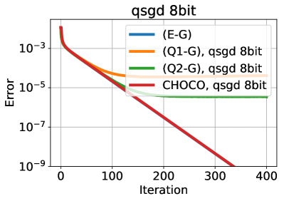
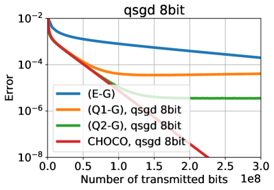
Figure 2: Average consensus on the ring topology with $n=25$ nodes, $d=2000$ coordinates and $(\operatorname{qsgd}_{256})$ compression

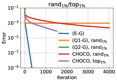
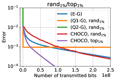
Figure 3: Average consensus on the ring topology with $n=25$ nodes, $d=2000$ coordinates and ($\operatorname{rand}_{1\%}$) and ($\operatorname{top}_{1\%}$) compression

dataset	$m$	$d$	density
epsilon	$400000$	$2000$	$100\%$
rcv1	$20242$	$47236$	$0.15\%$

Table 2: Size $(m,d)$ and density of the datasets.

experiment	$\gamma$
Choco, $(\operatorname{qsgd}_{256})$	1
Choco, ($\operatorname{rand}_{1\%}$)	0.011
Choco, ($\operatorname{top}_{1\%}$)	0.046

Table 3: Tuned stepsizes $\gamma$ for averaging in Figs. 3– 3.

	$epsilon$			$rcv1$
algorithm	$a$	$b$	$\gamma$	$a$	$b$	$\gamma$
Plain	0.1	$d$	-	1	1	-
Choco, $(\operatorname{qsgd}_{16})$	$0.1$	$d$	0.34	1	1	0.078
Choco, ($\operatorname{rand}_{1\%}$)	0.1	$d$	0.01	1	1	0.016
Choco, ($\operatorname{top}_{1\%}$)	0.1	$d$	0.04	1	1	0.04
DCD, ($\operatorname{rand}_{1\%}$)	$10^{-15}$	$d$	-	$10^{-10}$	$d$	-
DCD, $(\operatorname{qsgd}_{16})$	0.01	$d$	-	$10^{-10}$	$d$	-
ECD, ($\operatorname{rand}_{1\%}$)	$10^{-10}$	$d$	-	$10^{-10}$	$d$	-
ECD, ($\operatorname{qsgd}_{16}$)	$10^{-12}$	$d$	-	$10^{-10}$	$d$	-

Table 4: Parameters for the SGD learning rate $\eta_{t}=\frac{ma}{t+b}$ and consensus learning $\gamma$ used in the experiments in Figs. 5–6. Parameters where tuned separately for each algorithm. Tuning details can be found in Appendix F. The ECD and DCD stepsizes are small because the algorithms were observed to diverge for larger choices.

We compare the performance of the gossip schemes (E-G) (exact communication), (Q1-G), (Q2-G) (both with unbiased compression), and our scheme (Choco-G) in Figure 3 for the $(\operatorname{qsgd}_{256})$ compression scheme and in Figure 3 for the random ($\operatorname{rand}_{1\%}$) compression scheme. In addition, we also depict the performance of Choco-Gossip with biased ($\operatorname{top}_{1\%}$) compression. We use ring topology with uniformly averaging mixing matrix W as in Figure 1, left. The stepsizes $\gamma$ that were used for Choco-Gossip are listed in the Table 4. We consider here the consensus problem (2) with data $\mathbf{x}_{i}^{(0)}\in\mathbb{R}^{d}$ on the $i$-machine was chosen to be the $i$-th vector in the $epsilon$ dataset. We depict the errors $\tfrac{1}{n}\sum_{i=1}^{n}\bigl{\|}\mathbf{x}_{i}^{(t)}-\overline{\mathbf{x}}\bigr{\|}^{2}$.

The proposed scheme (Choco-G) with 8 bit quantization $(\operatorname{qsgd}_{256})$ converges with the same rate as (E-G) that uses exact communications (Fig. 3, left), while it requires much less data to be transmitted (Fig. 3, right). The schemes (Q1-G) and  (Q2-G) can do not converge and reach only accuracies of $10^{-4}$ –$10^{-5}$. The scheme (Q1-G) even starts to diverge, because the quantization error becomes larger than the optimization error.

With sparsified communication ($\operatorname{rand}_{1\%}$), i.e. transmitting only $1\%$ of all the coordinates, the scheme (Q1-G) quickly zeros out all the coordinates, and (Q2-G) diverges because quantization error is too large already from the first step (Fig. 3). Choco-Gossip proves to be more robust and converges. The observed rate matches with the theoretical findings, as we expect the scheme with factor $100\times$ compression to be $100\times$ slower than (E-G) without compression. In terms of total data transmitted, both schemes converge at the same speed (Fig. 3, right). We also see that ($\operatorname{rand}_{1\%}$) sparsification can give additional gains and comes out as the most data-efficient method in these experiments.

5.3 Decentralized SGD

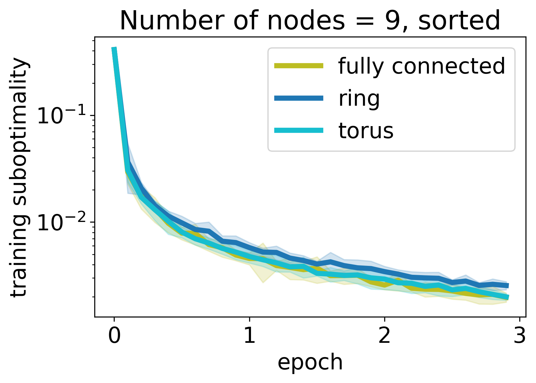
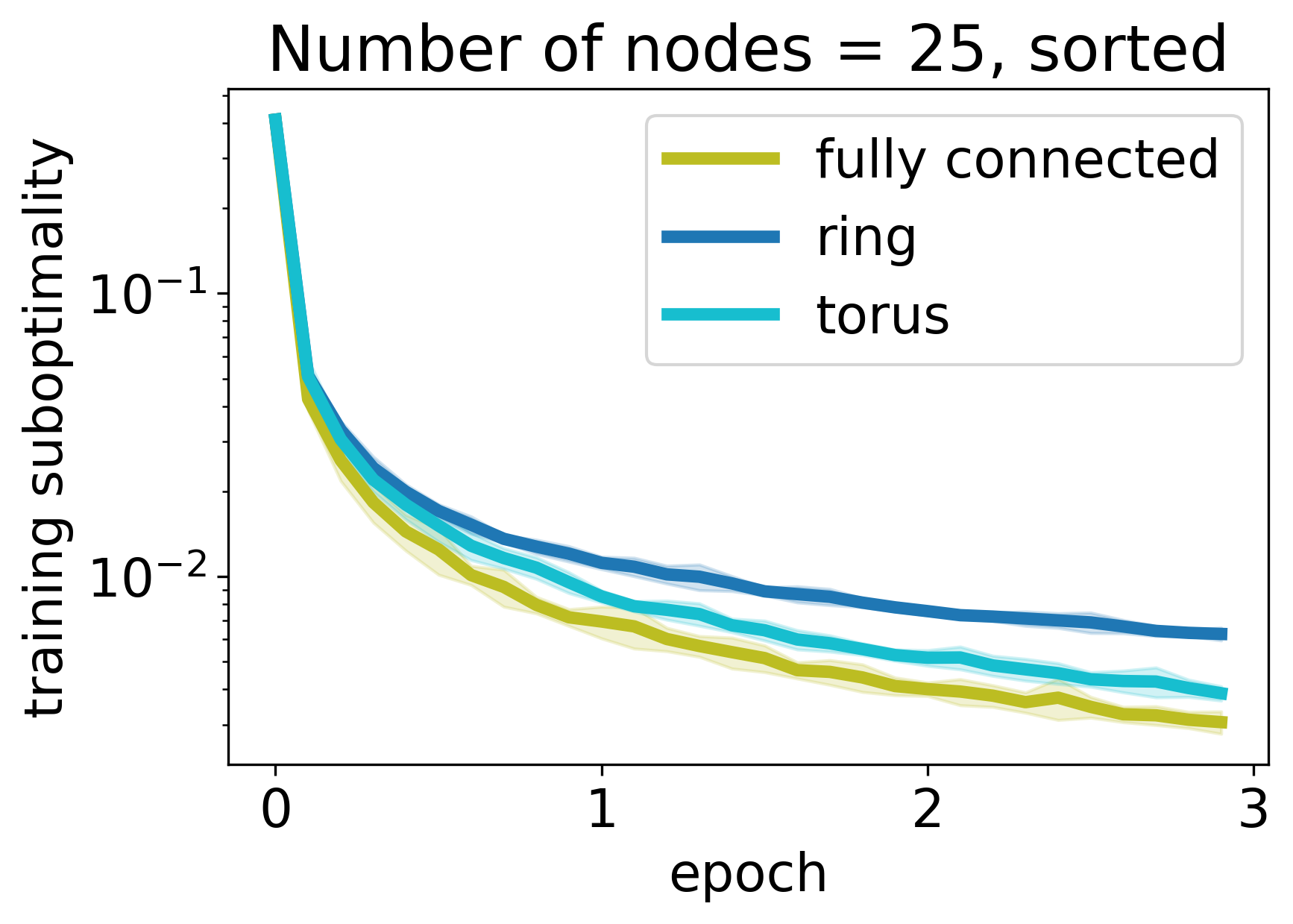
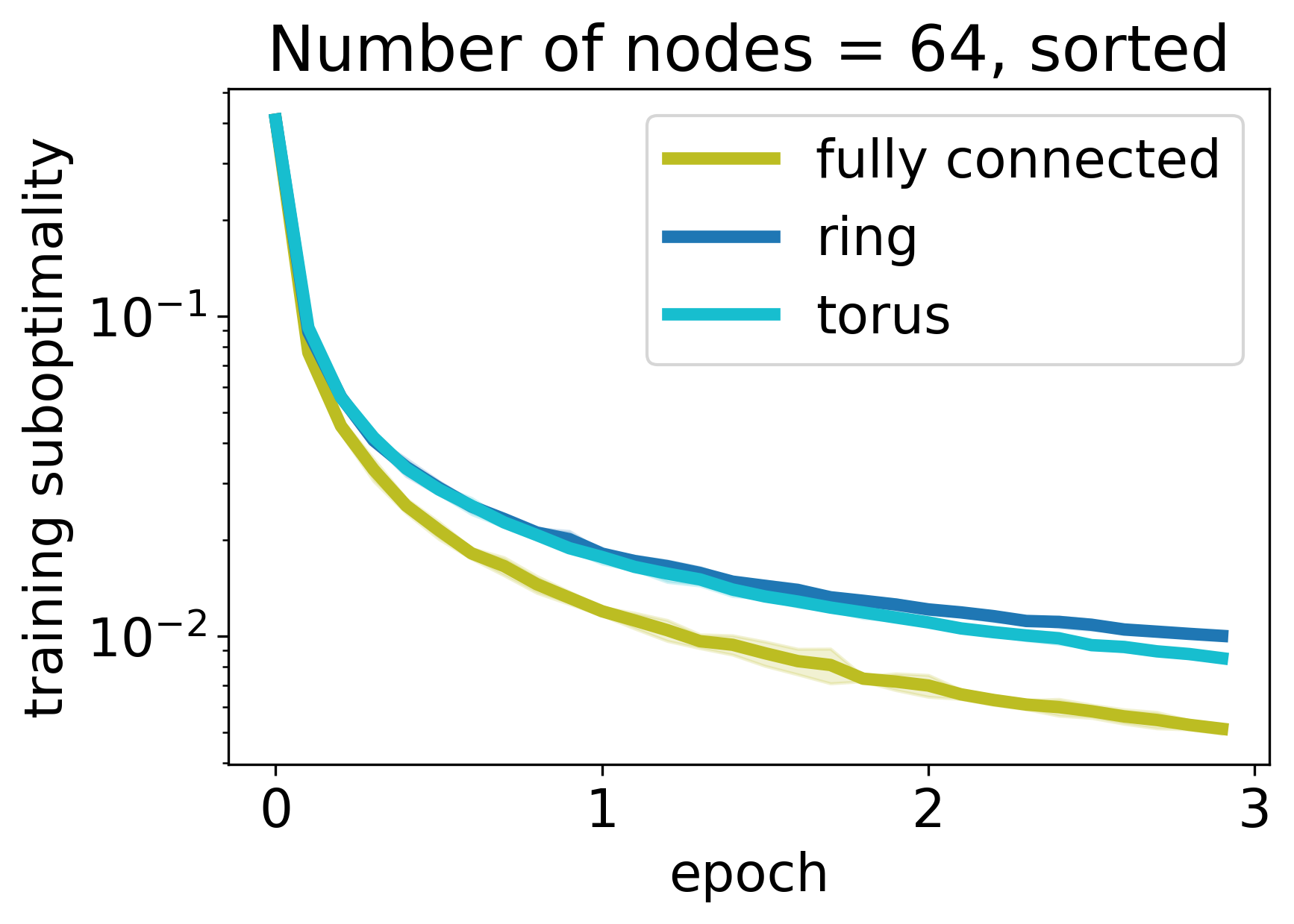
Figure 4: Performance of Algorithm 3 on ring, torus and fully connected topologies for $n\in\{9,25,64\}$ nodes. Here we consider the sorted setting, whilst the performance for randomly shuffled data is depicted in the Appendix G.

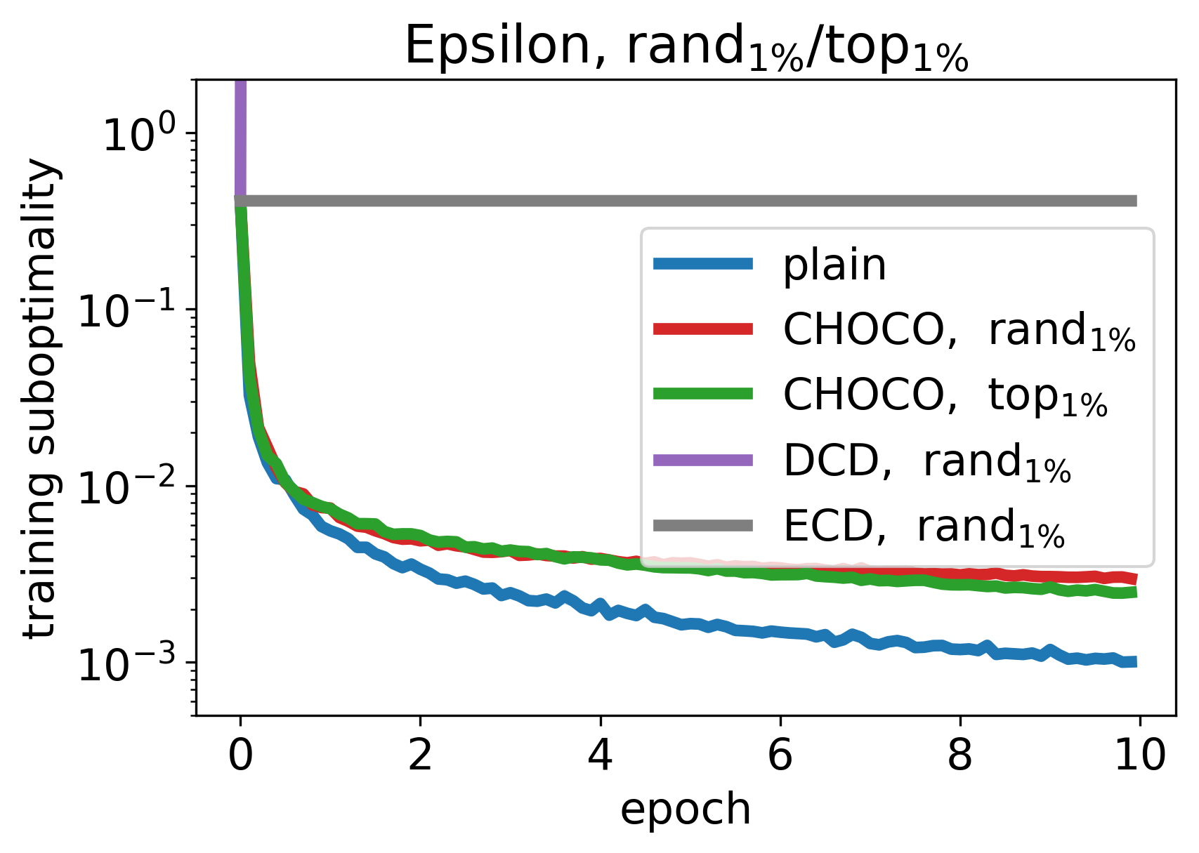
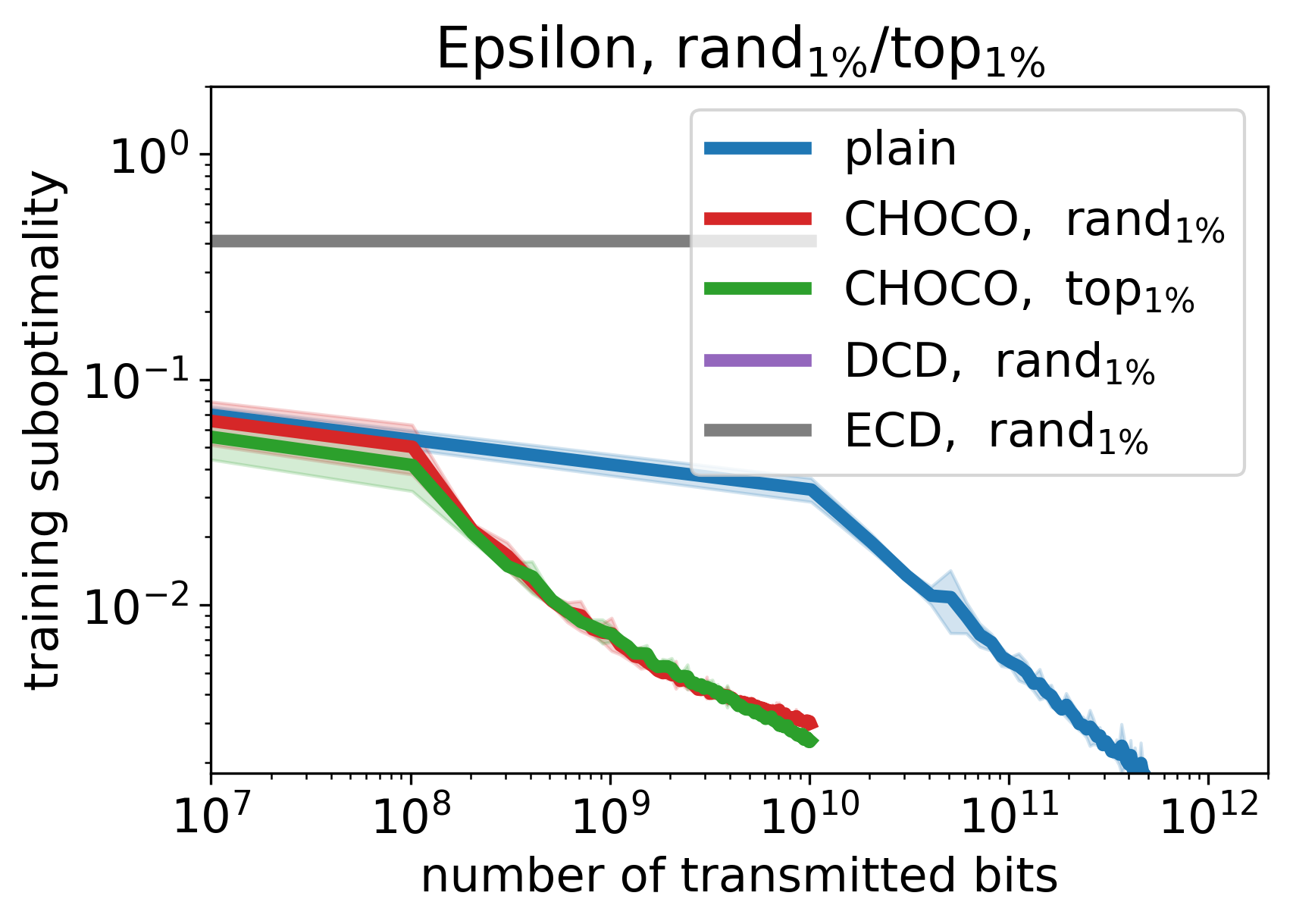
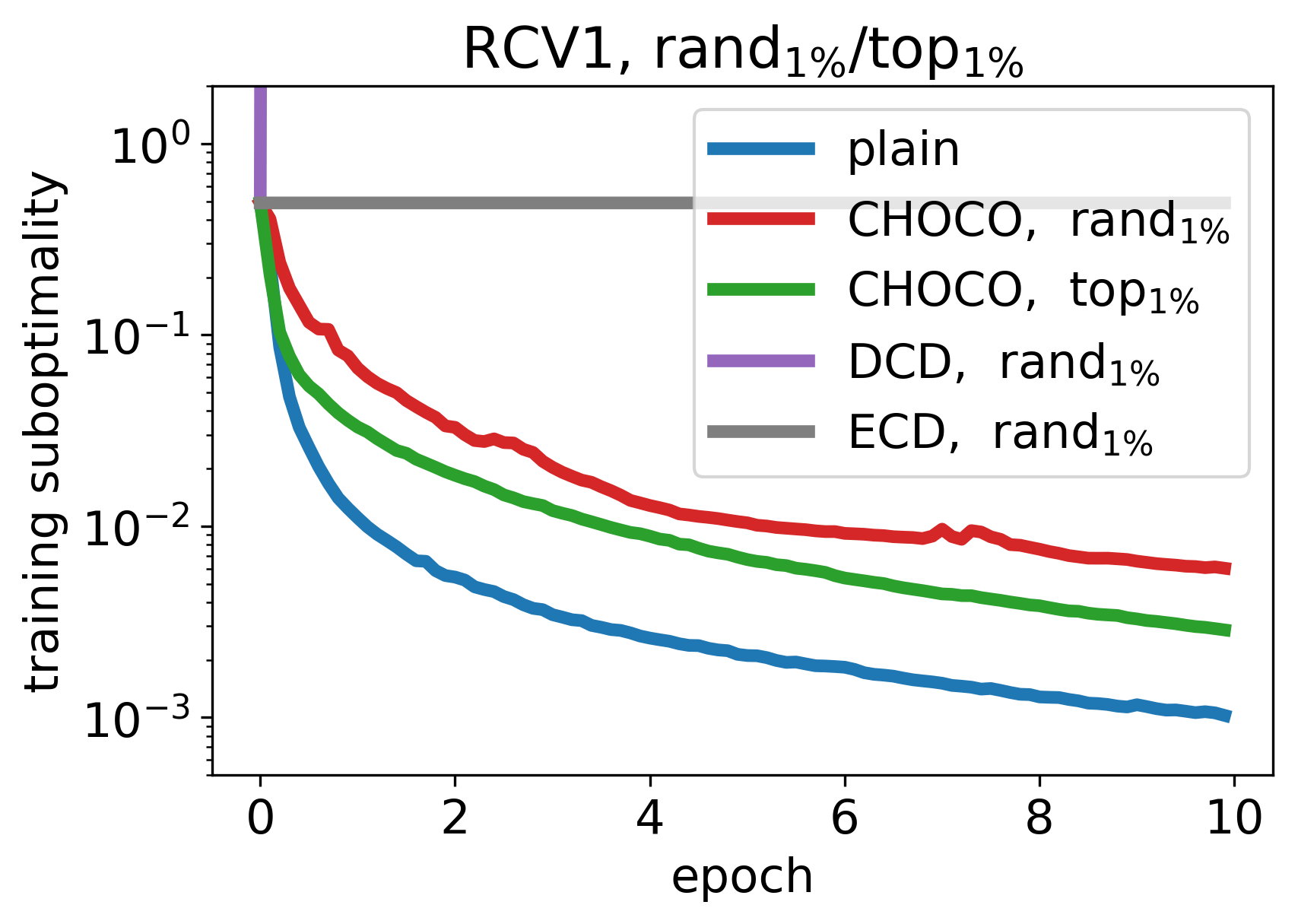
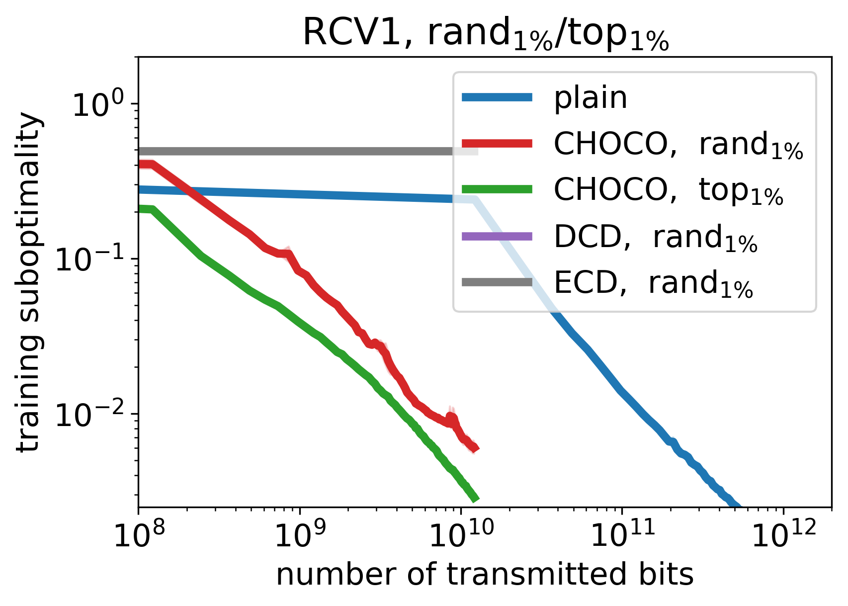
Figure 5: Comparison of Algorithm 3 (plain), ECD-SGD, DCD-SGD and Choco-SGD with ($\operatorname{rand}_{1\%}$) sparsification (in addition ($\operatorname{top}_{1\%}$) for Choco-SGD), for $epsilon$ (top) and $rcv1$ (bottom) in terms of iterations (left) and communication cost (right), $n=9$.

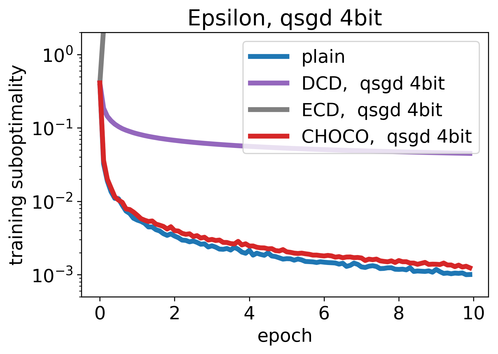
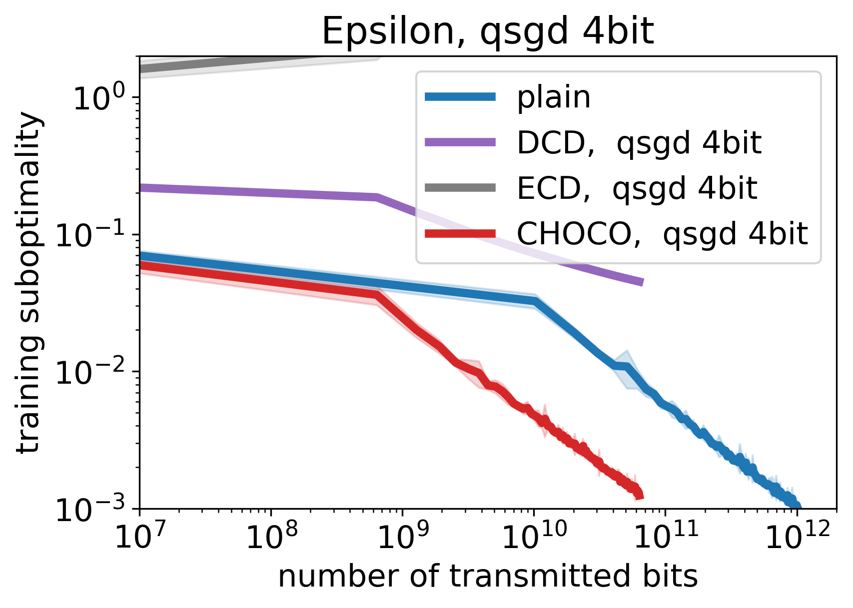
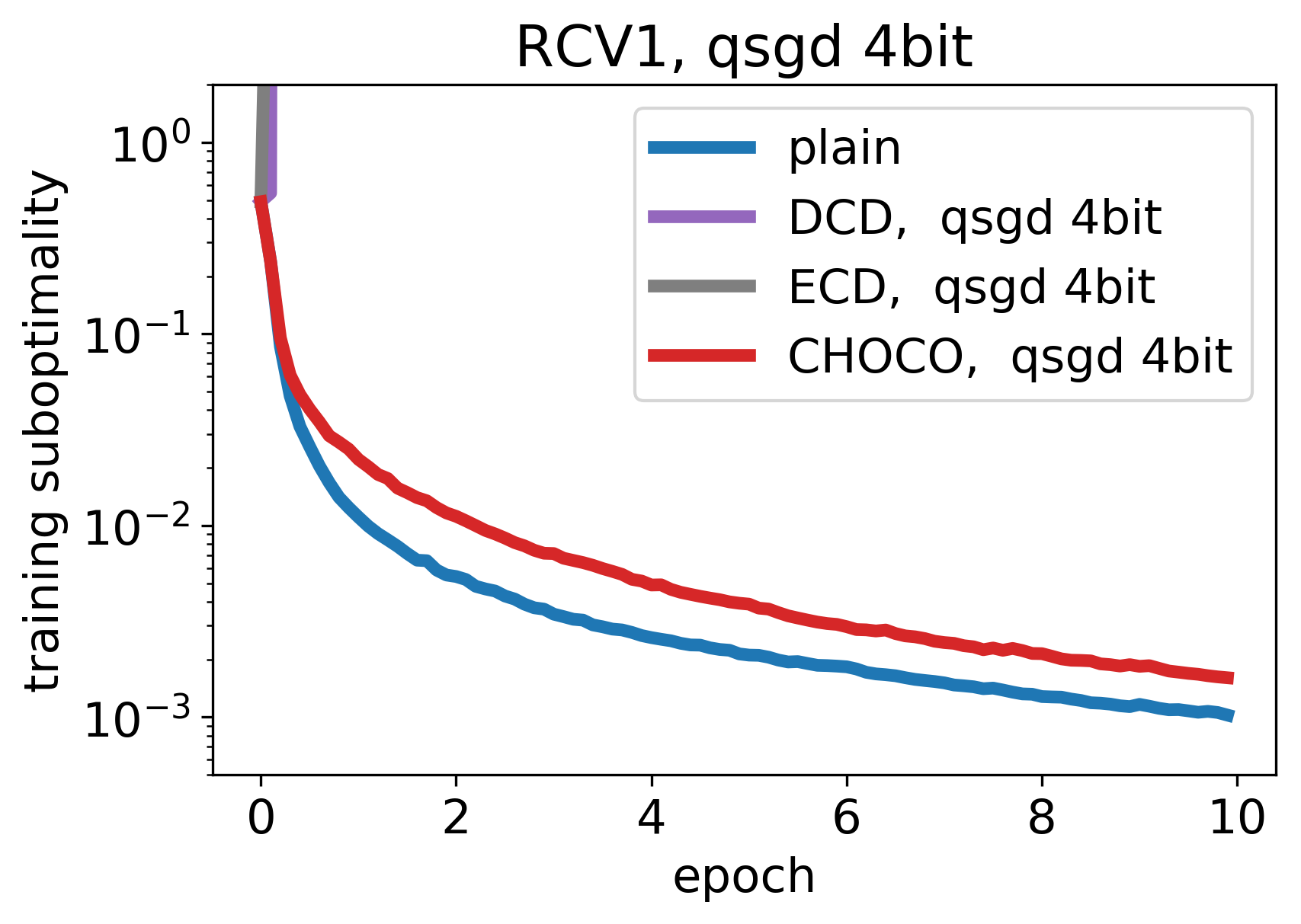
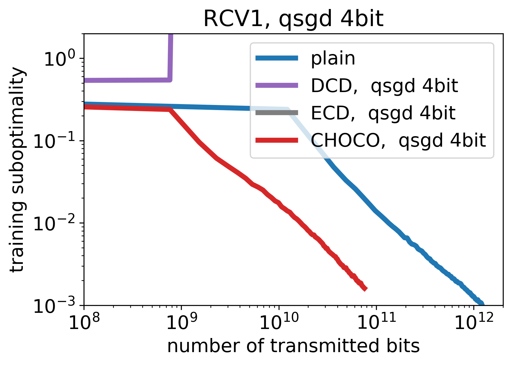
Figure 6: Comparison of Algorithm 3 (plain), ECD-SGD, DCD-SGD and Choco-SGD with ($\operatorname{qsgd}_{16}$) quantization, for $epsilon$ (top) and $rcv1$ (bottom) in terms of iterations (left) and communication cost (right), on $n=9$ nodes on a ring topology.

We asses the performance of Choco-SGD on logistic regression, defined as $\frac{1}{m}\sum_{j=1}^{m}\log(1+\exp(-b_{j}\mathbf{a}_{j}^{\top}\mathbf{x}))+\frac{1}{2m}\left\lVert\mathbf{x}\right\rVert^{2}$, where $\mathbf{a}_{j}\in\mathbb{R}^{d}$ and $b_{j}\in\{-1,1\}$ are the data samples and $m$ denotes the number of samples in the dataset. We distribute the $m$ data samples evenly among the $n$ workers and consider two settings: (i) randomly shuffled, where datapoints are randomly assigned to workers, and the more difficult (ii) sorted setting, where each worker only gets data samples just from one class (with the possible exception of one worker that gets two labels assigned). Moreover, we try to make the setting as difficult as possible, meaning that e.g. on the ring topology the machines with the same label form two connected clusters. We repeat each experiment three times and depict the mean curve and the area corresponding to one standard deviation. We plot suboptimality, i.e. $f(\overline{\mathbf{x}}^{(t)})-f^{\star}$ (obtained by $\operatorname{LogisticSGD}$ optimizer from scikit-learn Pedregosa et al. (2011)) versus number of iterations and the number of transmitted bits between workers, which is proportional to the actual running time if communication is a bottleneck.

Algorithms.

As baselines we consider Alg. 3 with exact communication (denoted as ‘plain’) and the communication efficient state-of-the-art optimization schemes DCD-SGD and ECD-SGD recently proposed in Tang et al. (2018a) (for unbiased quantization operators) and compare them to Choco-SGD. We use decaying stepsize $\eta_{t}=\frac{ma}{t+b}$ where the parameters $a,b$ are individually tuned for each algorithm and compression scheme, with values given in Table 4.

Impact of Topology.

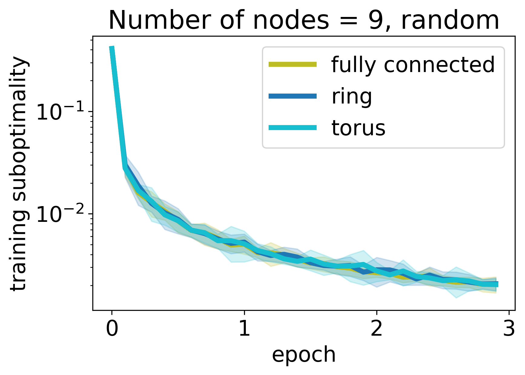
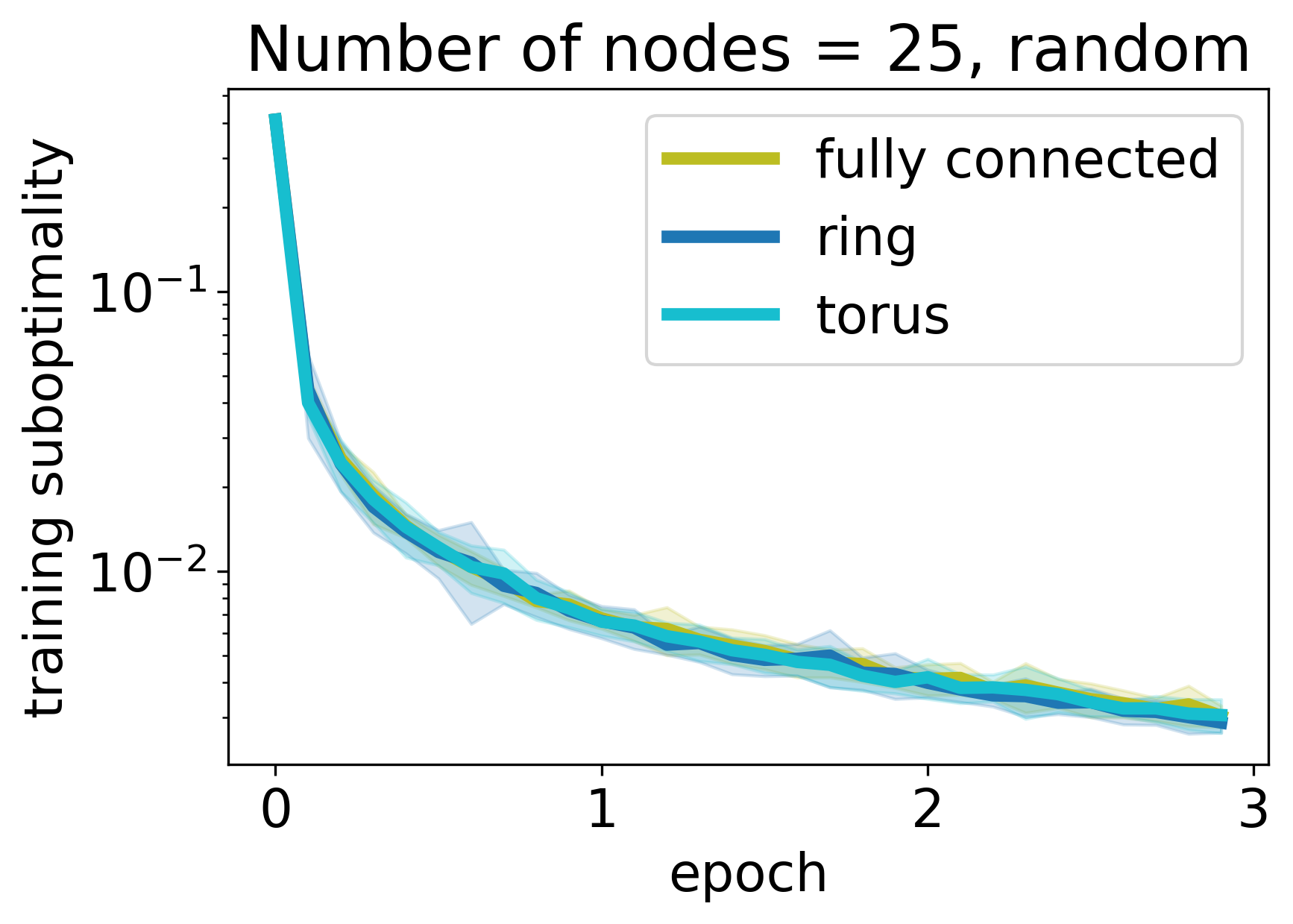
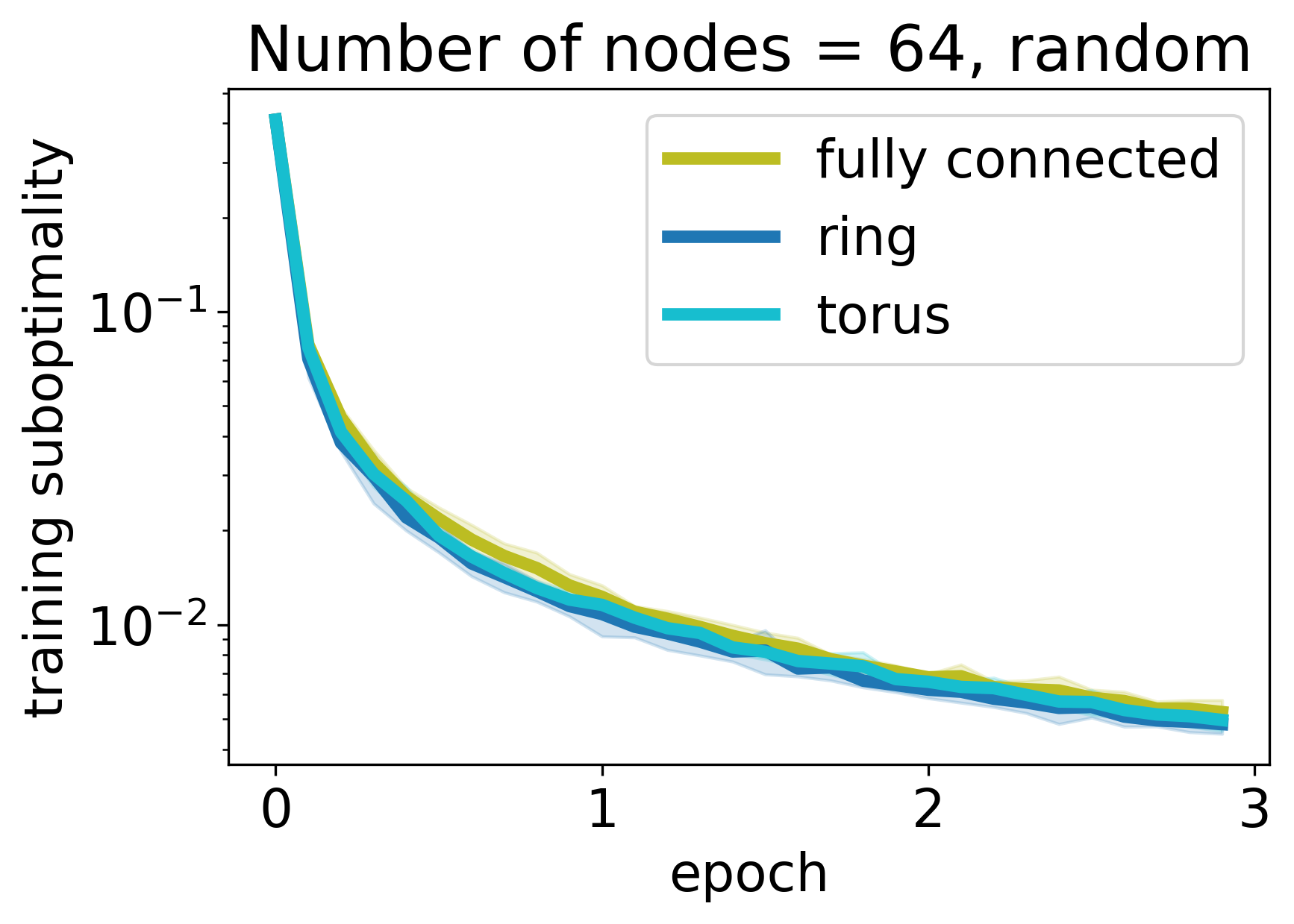
Figure 7: Performance of Algorithm 3 on ring, torus and fully connected topologies for $n\in\{9,25,64\}$ nodes. Randomly shuffled data between workers

In Figure 4 we depict the performance of the baseline Algorithm 3 with exact communication on different topologies (ring, torus and fully-connected; Fig. 1) with uniformly averaging mixing matrix $W$. Note that Algorithm 3 for fully-connected graph corresponds to mini-batch SGD. Increasing the number of workers from $n=9$ to $n=25$ and $n=64$ shows the mild effect of the network topology on the convergence. We observe that the sorted setting is more difficult than the randomly shuffled setting (see Fig. 7 in the Appendix G), where the convergence behavior remains almost unaffected. In the following we focus on the hardest case, i.e. the ring topology.

Comparison to Baselines.

In Figures 5 and 6 depict the performance of these algorithms on the ring topology with $n=9$ nodes for sorted data of the $epsilon$ and $rcv1$ datasets. Choco-SGD performs almost as good as the exact Algorithm 3 in all situations, but using $100\times$ less communication with ($\operatorname{rand}_{1\%}$) sparsification (Fig. 5, right) and approximately $15\times$ less communication for $(\operatorname{qsgd}_{4})$ quantization. The ($\operatorname{top}_{1\%}$) variant performs slightly better than ($\operatorname{rand}_{1\%}$) sparsification.

Choco-SGD consistently outperforms DCD-SGD in all settings. We also observed that DCD-SGD starts to perform better for larger number of levels $s$ in the $(\operatorname{qsgd}_{s})$ in the quantification operator (increasing communication cost). This is consistent with the reporting in Tang et al. (2018a) that assumed high precision quantization. As a surprise to us, ECD-SGD, which was proposed in Tang et al. (2018a) a the preferred alternative over DCD-SGD for less precise quantization operators, always performs worse than DCD-SGD, and often diverges.

Figures for randomly shuffled data and be found in the Appendix G. In that case Choco-SGD performs exactly as well as the exact Algorithm 3 in all situations.

Conclusion.

The experiments verify our theoretical findings: Choco-Gossip is the first linearly convergent gossip algorithm with quantized communication and Choco-SGD consistently outperforms the baselines for decentralized optimization, reaching almost the same performance as the exact algorithm without communication restrictions while significantly reducing communication cost. In view of the striking popularity of SGD as opposed to full-gradient methods for deep-learning, the application of Choco-SGD to decentralized deep learning—an instance of problem (1)— is a promising direction.

Acknowledgments.

We acknowledge funding from SNSF grant 200021_175796, as well as a Google Focused Research Award.

Appendix A Basic Identities and Inequalities

A.1 Smooth and Strongly Convex Functions

Definition 2.

A differentiable function $f\colon\mathbb{R}^{d}\to\mathbb{R}$ is $L$-strongly convex for parameter $L\geq 0$ if

$$f(\mathbf{y}) \leq f(\mathbf{x})+\left\langle\nabla f(\mathbf{x}),\mathbf{y}-\mathbf{x}\right\rangle+\frac{L}{2}\left\lVert\mathbf{y}-\mathbf{x}\right\rVert^{2}\,, \forall\mathbf{x},\mathbf{y}\in\mathbb{R}^{d}\,.$$ (9)

Definition 3.

A differentiable function $f\colon\mathbb{R}^{d}\to\mathbb{R}$ is $\mu$-strongly convex for parameter $\mu\geq 0$ if

$$f(\mathbf{y}) \geq f(\mathbf{x})+\left\langle\nabla f(\mathbf{x}),\mathbf{y}-\mathbf{x}\right\rangle+\frac{\mu}{2}\left\lVert\mathbf{y}-\mathbf{x}\right\rVert^{2}\,, \forall\mathbf{x},\mathbf{y}\in\mathbb{R}^{d}\,.$$ (10)

Remark 5.

If $f$ is $L$-smooth with minimizer $\mathbf{x}^{\star}$ s.t $\nabla f(\mathbf{x}^{\star})=\mathbf{0}$, then

$$\left\lVert\nabla f(\mathbf{x})\right\rVert^{2}=\left\lVert\nabla f(\mathbf{x})-\nabla f(\mathbf{x}^{\star})\right\rVert^{2}\leq 2L\left(f(\mathbf{x})-f(\mathbf{x}^{\star})\right)\,.$$ (11)

A.2 Vector and Matrix Inequalities

Remark 6.

For $A\in\mathbb{R}^{d\times n}$, $B\in\mathbb{R}^{n\times n}$

$$\left\lVert AB\right\rVert_{F}\leq\left\lVert A\right\rVert_{F}\left\lVert B\right\rVert_{2}\,.$$ (12)

Remark 7.

For arbitrary set of $n$ vectors $\{\mathbf{a}_{i}\}_{i=1}^{n}$, $\mathbf{a}_{i}\in\mathbb{R}^{d}$

$$\left\lVert\sum_{i=1}^{n}\mathbf{a}_{i}\right\rVert^{2}\leq n\sum_{i=1}^{n}\left\lVert\mathbf{a}_{i}\right\rVert^{2}\,.$$ (13)

Remark 8.

For given two vectors $\mathbf{a},\mathbf{b}\in\mathbb{R}^{d}$

$$2\left\langle\mathbf{a},\mathbf{b}\right\rangle\leq\gamma\left\lVert\mathbf{a}\right\rVert^{2}+\gamma^{-1}\left\lVert\mathbf{b}\right\rVert^{2}\,, \forall\gamma>0\,.$$ (14)

Remark 9.

For given two vectors $\mathbf{a},\mathbf{b}\in\mathbb{R}^{d}$

$$\left\lVert\mathbf{a}+\mathbf{b}\right\rVert^{2}\leq(1+\alpha)\left\lVert\mathbf{a}\right\rVert^{2}+(1+\alpha^{-1})\left\lVert\mathbf{b}\right\rVert^{2},\,\, \forall\alpha>0\,.$$ (15)

This inequality also holds for the sum of two matrices $A,B\in\mathbb{R}^{n\times d}$ in Frobenius norm.

A.3 Implications of the bounded gradient and bounded variance assumption

Remark 10.

If $F_{i}:\mathbb{R}^{d}\times\Omega\to\mathbb{R},i=1,\dots,n$ are convex functions with ${\mathbb{E}}_{\xi}\left.\left\lVert\nabla F_{i}(\mathbf{x},\xi)\right\rVert\right.^{2}\leq G^{2}$, $\partial F(X,\xi)=\left[\nabla F_{1}(\mathbf{x},\xi_{1}),\dots,\nabla F_{n}(\mathbf{x},\xi_{n})\right]$

$${\mathbb{E}}_{\xi_{1},\dots,\xi_{n}}\left.\left\lVert\partial F(X,\xi)\right\rVert_{F}^{2}\leq nG^{2}\right.,\,\, \forall X\,.$$

Remark 11 (Mini-batch variance).

If for functions $f_{i}$, $F_{i}$ defined in (8) ${\mathbb{E}}_{\xi}\left.\left\lVert\nabla F_{i}(\mathbf{x},\xi)-\nabla f_{i}(\mathbf{x})\right\rVert^{2}\right.\leq\sigma_{i}^{2},i\in[n]$, then

$${\mathbb{E}}_{\xi_{1}^{(t)},\dots,\xi_{n}^{(t)}}\left.\left\lVert\frac{1}{n}\sum_{j=1}^{n}\left(\nabla f_{j}(\mathbf{x}_{j}^{(t)})-\nabla F_{j}(\mathbf{x}_{j}^{(t)},\xi_{j}^{(t)})\right)\right\rVert\right.^{2}\leq\dfrac{\overline{\sigma}^{2}}{n},$$

where $\overline{\sigma}^{2}=\frac{\sum_{i=1}^{n}\sigma_{i}^{2}}{n}$.

Proof.

This follows from

$${\mathbb{E}}\left.\left\lVert\frac{1}{n}\sum_{j=1}^{n}Y_{j}\right\rVert\right.^{2}=\dfrac{1}{n^{2}}\left(\sum_{j=1}^{n}{\mathbb{E}}\left.\left\lVert Y_{j}\right\rVert\right.^{2}+\sum_{i\neq j}{\mathbb{E}}\left.\left\langle Y_{i},Y_{j}\right\rangle\right.\right)=\dfrac{1}{n^{2}}\sum_{j=1}^{n}{\mathbb{E}}\left.\left\lVert Y_{j}\right\rVert\right.^{2}\leq\frac{1}{n^{2}}\sum_{j=1}^{n}\sigma_{j}^{2}=\dfrac{\overline{\sigma}^{2}}{n}$$

for $Y_{j}=f_{j}(\mathbf{x}_{j}^{(t)})-\nabla F_{j}(\mathbf{x}_{j}^{(t)},\xi_{j}^{(t)})$. Expectation of scalar product is equal to zero because $\xi_{i}$ is independent of $\xi_{j}$ since $i\neq j$. ∎

Appendix B Consensus in Matrix notation

In the proofs in the next section we will use the matrix notation, as already introduced in the main text. We define

$$X^{(t)} :=\left[\mathbf{x}_{1}^{(t)},\dots,\mathbf{x}_{n}^{(t)}\right]\in\mathbb{R}^{d\times n}, Q^{(t)}:=\left[\mathbf{q}_{1}^{(t)},\dots,\mathbf{q}_{n}^{(t)}\right]\in\mathbb{R}^{d\times n}, \hat{X}^{(t)}:=\left[\hat{\mathbf{x}}_{1}^{(t)},\dots,\hat{\mathbf{x}}_{n}^{(t)}\right]\in\mathbb{R}^{d\times n}\,.$$ (16)

Then using matrix notation we can rewrite Algorithm 1 as

Algorithm 1 Choco-Gossip in matrix notation

0:  : $X^{(0)}$, $\gamma$, $W$.

1:  Initialize: $\hat{X}^{(0)}=0$

2:  for $t$ in $0\dots T-1$ do

3:     $Q^{(t)}=Q(X^{(t)}-\hat{X}^{(t)})$

4:     $\hat{X}^{(t+1)}=\hat{X}^{(t)}+Q^{(t)}$

5:     $X^{(t+1)}=X^{(t)}+\gamma\hat{X}^{(t+1)}\left(W-I\right)$

6:  end for

Remark 12.

Note that since every worker $i$ for each neighbor $j:\{i,j\}\in E$ stores $\hat{\mathbf{x}}_{j}$, the proper notation for $\hat{\mathbf{x}}$ would be to use $\hat{\mathbf{x}}_{ij}$ instead. We simplified it using the property that if $\hat{\mathbf{x}}_{ij}^{(0)}=\hat{\mathbf{x}}_{kj}^{(0)}$, $\forall i,k:\{i,j\}\in E$ and $\{k,j\}\in E$, then they are equal at all timesteps $\hat{\mathbf{x}}_{ij}^{(t)}=\hat{\mathbf{x}}_{kj}^{(t)}$, $\forall t\geq 0$.

Remark 13.

The results of Theorem 4 and 19 also hold for arbitrary initialized $\hat{X}^{(0)}$ with the constraint that $\forall j$ all the neighbors of the node $j$ initialized with the same $\hat{\mathbf{x}}_{i}$, i.e. using extended notation $\hat{\mathbf{x}}_{ij}^{(0)}=\hat{\mathbf{x}}_{kj}^{(0)}$, $\forall i,k:\{i,j\}\in E$ and $\{k,j\}\in E$.

B.1 Useful Facts

Remark 14.

Let $X^{(t)}=\left[\mathbf{x}_{1}^{(t)},\dots,\mathbf{x}_{n}^{(t)}\right]\in\mathbb{R}^{d\times n}$ and $\overline{X}^{(t)}=\left[\overline{\mathbf{x}}^{(t)},\dots,\overline{\mathbf{x}}^{(t)}\right]\in\mathbb{R}^{d\times n}$, for $\overline{\mathbf{x}}^{(t)}=\frac{1}{n}\sum_{i=1}^{n}\mathbf{x}_{i}^{(t)}$, then because $W$ is doubly stochastic

$$\overline{X}^{(t)}=X^{(t)}\frac{1}{n}\mathbf{1}\mathbf{1}^{\top}, \overline{X}^{(t)}W=\overline{X}^{(t)}\,.$$ (17)

Remark 15.

The average $\overline{X}^{(t)}=\left[\overline{\mathbf{x}}^{(t)},\dots,\overline{\mathbf{x}}^{(t)}\right]\in\mathbb{R}^{d\times n}$ during iterates of the Algorithm 1 is preserved, i.e.

$$\overline{X}^{(t)}=\overline{X}^{(0)},\quad\forall t,$$ (18)

where $\overline{X}^{(t)}=\left[\overline{\mathbf{x}}^{(t)}\dots,\overline{\mathbf{x}}^{(t)}\right]\in\mathbb{R}^{d\times n}$.

Proof.

$$\overline{X}^{(t+1)}=\overline{X}^{(t)}+\gamma\hat{X}^{(t)}\left(W-I\right)\frac{\mathbf{1}\mathbf{1}^{\top}}{n}=\overline{X}^{(t)},$$

because $W\frac{\mathbf{1}\mathbf{1}^{\top}}{n}=I$ since $W$ is doubly stochastic. ∎

Lemma 16.

For $W$ satisfying Definition 1, i.e. W is symmetric doubly stochastic matrix with second largest eigenvalue $1-\delta=|\lambda_{2}(W)|<1$

$$\left\lVert W^{k}-\frac{1}{n}\mathbf{1}\mathbf{1}^{\top}\right\rVert_{2}\leq(1-\delta)^{k}\,.$$ (19)

Proof.

Let $U\Lambda U^{\top}$ be SVD-decomposition of $W$, then $W^{k}=U\Lambda^{k}U^{\top}$ Because of the stochastic property of $W$ its first eigenvector is $u_{1}=\frac{1}{\sqrt{n}}\mathbf{1}$.

$$U\begin{pmatrix}1&0&\dots&0\\ 0&0&\dots&0\\ \dots\\ 0&0&\dots&0\\ \end{pmatrix}U^{\top}=u_{1}u_{1}^{\top}=\dfrac{1}{n}\mathbf{1}\mathbf{1}^{\top}$$

Hence,

$$\left\lVert W^{k}-\frac{1}{n}\mathbf{1}\mathbf{1}^{\top}\right\rVert_{2} =\left\lVert U\Lambda^{k}U^{\top}-U\begin{pmatrix}1&0&\dots&0\\ 0&0&\dots&0\\ \dots\\ 0&0&\dots&0\\ \end{pmatrix}U^{\top}\right\rVert_{2}=\left\lVert\Lambda^{k}-\begin{pmatrix}1&0&\dots&0\\ 0&0&\dots&0\\ \dots\\ 0&0&\dots&0\\ \end{pmatrix}\right\rVert_{2}=(1-\delta)^{k}.\qed$$

Appendix C Proof of Theorem 2—Convergence of Choco-Gossip

Lemma 17.

Let $X^{(t)},\hat{X}^{(t)}\in\mathbb{R}^{d\times n}$, $\overline{X}=[\overline{\mathbf{x}},\dots,\overline{\mathbf{x}}]$ for average $\overline{\mathbf{x}}=\frac{1}{n}X^{(t)}\mathbf{1}\in\mathbb{R}^{d}$ and let $X^{(t+1)}=X^{(t)}+\gamma\hat{X}^{(t)}(W-I)\in\mathbb{R}^{d\times n}$ be defined as in Algorithm 1 with stepsize $\gamma\geq 0$ and mixing matrix $W\in\mathbb{R}^{n\times n}$ as in Definition 1. Then

$$\left\lVert X^{(t+1)}-\overline{X}\right\rVert^{2}_{F}\leq(1-\delta\gamma)^{2}(1+\alpha_{1})\left\lVert X^{(t)}-\overline{X}\right\rVert_{F}^{2}+\gamma^{2}(1+\alpha_{1}^{-1})\beta^{2}\left\lVert\hat{X}^{(t+1)}-X^{(t)}\right\rVert_{F}^{2},\,\,\forall\alpha_{1}>0\,.$$

Here $\alpha_{1}>0$ is a parameter whose value will be chosen later, $\delta=1-|\lambda_{2}(W)|$ and $\beta=\max_{i}\{1-\lambda_{i}(W)\}$ as defined above.

Proof.

By the definition of $X^{(t+1)}$ and the observation $\overline{X}(W-I)=0$, we can write

$$\left\lVert X^{(t+1)}-\overline{X}\right\rVert_{F}^{2} =\left\lVert X^{(t)}-\overline{X}+\gamma\hat{X}^{(t+1)}(W-I)\right\rVert^{2}_{F}$$

$$=\left\lVert X^{(t)}-\overline{X}+\gamma\left(X^{(t)}-\overline{X}\right)(W-I)+\gamma\left(\hat{X}^{(t+1)}-X^{(t)}\right)(W-I)\right\rVert_{F}^{2}$$

$$=\left\lVert\left(X^{(t)}-\overline{X}\right)((1-\gamma)I+\gamma W)+\gamma\left(\hat{X}^{(t+1)}-X^{(t)}\right)(W-I)\right\rVert^{2}_{F}$$

$$\stackrel{{\scriptstyle\eqref{eq:norm_of_sum_of_two}}}{{\leq}}(1+\alpha_{1})\left\lVert\left(X^{(t)}-\overline{X}\right)((1-\gamma)I+\gamma W)\right\rVert_{F}^{2}+(1+\alpha_{1}^{-1})\left\lVert\gamma\left(\hat{X}^{(t+1)}-X^{(t)}\right)(W-I)\right\rVert^{2}_{F}$$

$$\stackrel{{\scriptstyle\text{\eqref{eq:frob_norm_of_multiplication}}}}{{\leq}}(1+\alpha_{1})\left\lVert\left(X^{(t)}-\overline{X}\right)((1-\gamma)I+\gamma W)\right\rVert^{2}_{F}+(1+\alpha_{1}^{-1})\gamma^{2}\left\lVert W-I\right\rVert_{2}^{2}\cdot\left\lVert\hat{X}^{(t+1)}-X^{(t)}\right\rVert^{2}_{F}\,.$$

Let’s estimate the first term

$$\left\lVert\left(X^{(t)}-\overline{X}\right)((1-\gamma)I+\gamma W)\right\rVert_{F} \leq(1-\gamma)\left\lVert X^{(t)}-\overline{X}\right\rVert_{F}+\gamma\left\lVert\left(X^{(t)}-\overline{X}\right)W\right\rVert_{F}$$

$$\stackrel{{\scriptstyle\text{\eqref{eq:average}}}}{{=}}(1-\gamma)\left\lVert X^{(t)}-\overline{X}\right\rVert_{F}+\gamma\left\lVert\left(X^{(t)}-\overline{X}\right)\left(W-\mathbf{1}\mathbf{1}^{\top}/n\right)\right\rVert_{F}$$

$$\stackrel{{\scriptstyle\text{\eqref{eq:mixing_matrix}, \eqref{eq:frob_norm_of_multiplication} }}}{{\leq}}(1-\gamma\delta)\left\lVert X^{(t)}-\overline{X}\right\rVert_{F}$$

where we used $(X^{(t)}-\overline{X})\mathbf{1}\mathbf{1}^{\top}/n=0$, by definition of $\overline{X}$, in the second line. Putting this together gives us the statement of the lemma. ∎

Lemma 18.

Let $X^{(t)},\hat{X}^{(t)}\in\mathbb{R}^{d\times n}$, $\overline{X}=[\overline{\mathbf{x}},\dots,\overline{\mathbf{x}}]$ for average $\overline{\mathbf{x}}=\frac{1}{n}X^{(t)}\mathbf{1}\in\mathbb{R}^{d}$ and let $X^{(t+1)}\in\mathbb{R}^{d\times n}$ and $\hat{X}^{(t+2)}\in\mathbb{R}^{d\times n}$ be defined as in Algorithm 1 with stepsize $\gamma\geq 0$, mixing matrix $W\in\mathbb{R}^{n\times n}$ as in Definition 1 and quantization as in Assumption 1. Then

$${\mathbb{E}}_{Q}\left.\left\lVert X^{(t+1)}-\hat{X}^{(t+2)}\right\rVert^{2}_{F}\right. \leq(1-\omega)(1+\gamma\beta)^{2}(1+\alpha_{2})\left\lVert X^{(t)}-\hat{X}^{(t+1)}\right\rVert^{2}_{F}$$

$$+(1-\omega)\gamma^{2}\beta^{2}(1+\alpha_{2}^{-1})\left\lVert X^{(t)}-\overline{X}\right\rVert_{F}^{2},\,\, \forall\alpha_{2}>0\,.$$

Here $\alpha_{2}>0$ is a parameter whose value will be chosen later, $\beta=\max_{i}\{1-\lambda_{i}(W)\}$ as defined above and compression ratio $\omega>0$.

Proof.

By the definition of $X^{(t+1)}$ and $\hat{X}^{(t+2)}$ we can write

$${\mathbb{E}}_{Q}\left.\left\lVert X^{(t+1)}-\hat{X}^{(t+2)}\right\rVert^{2}_{F}\right. ={\mathbb{E}}_{Q}\left.\left\lVert X^{(t+1)}-\hat{X}^{(t+1)}-Q(X^{(t+1)}-\hat{X}^{(t+1)})\right\rVert_{F}^{2}\right.\stackrel{{\scriptstyle\text{\eqref{def:omega}}}}{{\leq}}(1-\omega)\left\lVert X^{(t+1)}-\hat{X}^{(t+1)}\right\rVert_{F}^{2}$$

$$=(1-\omega)\left\lVert X^{(t)}+\gamma\hat{X}^{(t+1)}(W-I)-\hat{X}^{(t+1)}\right\rVert_{F}^{2}$$

$$\stackrel{{\scriptstyle\text{\eqref{eq:average}}}}{{=}}(1-\omega)\left\lVert\left(X^{(t)}-\hat{X}^{(t+1)}\right)\left((1+\gamma)I-\gamma W\right)+\gamma(W-I)\left({X}^{(t)}-\overline{X}\right)\right\rVert_{F}^{2}$$

$$\stackrel{{\scriptstyle\text{\eqref{eq:norm_of_sum_of_two}}}}{{\leq}}(1-\omega)(1+\alpha_{2})\left\lVert\left(X^{(t)}-\hat{X}^{(t+1)}\right)\left((1+\gamma)I-\gamma W\right)\right\rVert_{F}^{2}$$

$$\hskip 28.45274pt+(1-\omega)(1+\alpha_{2}^{-1})\left\lVert\gamma(W-I)\left({X}^{(t)}-\overline{X}\right)\right\rVert_{F}^{2}$$

$$\stackrel{{\scriptstyle\text{\eqref{eq:frob_norm_of_multiplication}}}}{{\leq}}(1-\omega)(1+\gamma\beta)^{2}(1+\alpha_{2})\left\lVert X^{(t)}-\hat{X}^{(t+1)}\right\rVert_{F}^{2}+(1-\omega)\gamma^{2}\beta^{2}(1+\alpha_{2}^{-1})\left\lVert X^{(t)}-\overline{X}\right\rVert_{F}^{2}\,,$$

where we used $\left\lVert I+\gamma(I-W)\right\rVert_{2}=1+\gamma\left\lVert I-W\right\rVert_{2}=1+\gamma\beta$ because eigenvalues of $\gamma(I-W)$ are positive. ∎

Proof of Theorem 2.

As observed in Remark 14 the averages of the iterates is preserved, i.e. $\overline{X}\equiv X^{(t)}\frac{1}{n}\mathbf{1}\mathbf{1}^{\top}$ for all $t\geq 0$. By applying the Lemmas 17 and 18 from above we obtain

$${\mathbb{E}}_{Q}\left.e_{t+1}\right. \leq\eta_{1}(\gamma)\left\lVert X^{(t)}-\overline{X}\right\rVert_{F}^{2}+\xi_{1}(\gamma)\left\lVert\hat{X}^{(t+1)}-X^{(t)}\right\rVert_{F}^{2}\leq\max\{\eta_{1}(\gamma),\xi_{1}(\gamma)\}\cdot e_{t}\,,$$

where

$$\eta_{1}(\gamma) :=(1-\delta\gamma)^{2}(1+\alpha_{1})+(1-\omega)\gamma^{2}\beta^{2}(1+\alpha_{2}^{-1})\,,$$

$$\xi_{1}(\gamma) :=\gamma^{2}\beta^{2}(1+\alpha_{1}^{-1})+(1-\omega)(1+\gamma\beta)^{2}(1+\alpha_{2})\,.$$

Now, we need to choose the parameters $\alpha_{1},\alpha_{2}$ and stepsize $\gamma$ such as to minimize the factor $\max\{\eta_{1}(\gamma),\xi_{1}(\gamma)\}$. Whilst the optimal parameter settings can for instance be obtained using specialized optimization software, we here proceed by showing that for the (suboptimal) choice

$$\begin{split}\alpha_{1}&:=\frac{\gamma\delta}{2},\\ \alpha_{2}&:=\frac{\omega}{2}\\ \gamma^{\star}&:=\frac{\delta\omega}{16\delta+\delta^{2}+4\beta^{2}+2\delta\beta^{2}-8\delta\omega}\end{split}$$ (20)

it holds

$$\max\{\eta_{1}(\gamma^{\star}),\xi_{1}(\gamma^{\star})\} \leq 1-\frac{\delta^{2}\omega}{2(16\delta+\delta^{2}+4\beta^{2}+2\delta\beta^{2}-8\delta\omega)}\,.$$ (21)

The claim of the theorem then follows by observing

$$1-\frac{\delta^{2}\omega}{2(16\delta+\delta^{2}+4\beta^{2}+2\delta\beta^{2}-8\delta\omega)}\leq 1-\frac{\delta^{2}\omega}{82}\,,$$ (22)

using the crude estimates $0\leq\delta\leq 1$, $\beta\leq 2$, $\omega\geq 0$.

We now proceed to show that (21) holds. Observe that for $\alpha_{1},\alpha_{2}$ as in (20),

$$\eta_{1}(\gamma) \leq\left(1-\gamma\delta\right)\left(1-\gamma\delta\right)\left(1+\frac{\gamma\delta}{2}\right)+\gamma^{2}\beta^{2}(1-\omega)\left(1+\frac{2}{\omega}\right)$$

$$\leq\left(1-\frac{\gamma\delta}{2}\right)^{2}+\frac{2}{\omega}\gamma^{2}\beta^{2}=:\eta_{2}(\gamma)\,,$$

where we used the inequality $(1-x)(1+\frac{x}{2})\leq(1-\frac{x}{2})$ and $(1-\omega)(1+2/\omega)\leq\frac{2}{\omega}$ for $\omega>0$. The quadratic function $\eta_{2}(\gamma)$ is minimized for $\gamma^{\prime}=\frac{2\delta\omega}{8\beta^{2}+\delta^{2}\omega}$ with value $\eta_{2}(\gamma^{\prime})=\frac{8\beta^{2}}{8\beta^{2}+\delta^{2}\omega}<1$. Thus by Jensen’s inequality

$$\eta_{2}(\lambda\gamma^{\prime})\leq(1-\lambda)\eta_{2}(0)+\lambda\eta_{2}(\gamma^{\prime})=1-\lambda\frac{\delta^{2}\omega}{8\beta^{2}+\delta^{2}\omega}$$ (23)

for $0\leq\lambda\leq 1$, and especially for the choice $\lambda^{\prime}=\frac{8\beta^{2}+\delta^{2}\omega}{2(16\delta+\delta^{2}+4\beta^{2}+2\delta\beta^{2}-8\delta\omega)}$ we have

$$\eta_{1}(\gamma^{\star})\leq\eta_{2}(\lambda^{\prime}\gamma^{\prime})\stackrel{{\scriptstyle\eqref{eq:3455}}}{{\leq}}1-\frac{\delta^{2}\omega}{2(16\delta+\delta^{2}+4\beta^{2}+2\delta\beta^{2}-8\delta\omega)}\,,$$ (24)

as $\gamma^{\star}=\lambda^{\prime}\gamma^{\prime}$. Now we proceed to estimate $\xi_{1}(\gamma^{\star})$. Observe

$$\xi_{1}(\gamma) \leq\gamma^{2}\beta^{2}\left(1+\frac{2}{\gamma\delta}\right)+(1+\gamma\beta)^{2}(1-\omega)\left(1+\frac{\omega}{2}\right)\leq\gamma^{2}\beta^{2}\left(1+\frac{2}{\gamma\delta}\right)+(1+\gamma\beta)^{2}\left(1-\frac{\omega}{2}\right)\,,$$ (25)

again from $(1-x)(1+\frac{x}{2})\leq(1-\frac{x}{2})$ for $x>0$. As $\beta\leq 2$ we can estimate $(1+\gamma\beta)^{2}\leq 1+8\gamma$ for any $0\leq\gamma\leq 1$. Furthermore $\gamma^{2}\leq\gamma$ for $0\leq\gamma\leq 1$. Thus

$$\xi_{1}(\gamma^{\star})\leq\beta^{2}\left(\gamma^{\star}+\frac{2\gamma^{\star}}{\delta}\right)+\left(1-\frac{\omega}{2}\right)(1+8\gamma^{\star})=1-\frac{\delta^{2}\omega}{2(16\delta+\delta^{2}+4\beta^{2}+2\delta\beta^{2}-8\delta\omega)}\,,$$ (26)

as a quick calculation shows. ∎

Appendix D Proof of Theorem 4—Convergence of Choco-SGD

Recall, that $\bigl{\{}\mathbf{x}_{i}^{(t)}\}_{t=0}^{T}$ denote the iterates of Algorithm 2 on worker $i\in[n]$. We define

$$\overline{\mathbf{x}}^{(t)}:=\frac{1}{n}\sum_{i=1}^{n}\mathbf{x}_{i}^{(t)}\,,$$ (27)

the average over all workers. Note that this quantity is not available to the workers at any given time, but it will be conveniently to use for the proofs. In this section we use both vector and matrix notation whenever it is more convenient, and define

$$\begin{split}X^{(t)}:=\left[\mathbf{x}_{1}^{(t)},\dots,\mathbf{x}_{n}^{(t)}\right]\in\mathbb{R}^{d\times n},\qquad\overline{X}^{(t)}:=\left[\overline{\mathbf{x}}^{(t)},\dots,\overline{\mathbf{x}}^{(t)}\right]\in\mathbb{R}^{d\times n},\\ \partial F(X^{(t)},\xi^{(t)}):=\left[\nabla F_{1}(\mathbf{x}_{1}^{(t)},\xi_{1}^{(t)}),\dots,\nabla F_{n}(\mathbf{x}_{n}^{(t)},\xi_{n}^{(t)})\right]\in\mathbb{R}^{d\times n}.\end{split}$$ (28)

Instead of proving Theorem 4 directly, we prove a slightly more general statement in this section. Algorithm 2 relies on the (compressed) consensus Algorithm 1. However, we can also show convergence of Algorithm 2 for more general averaging schemes. In Algorithm 4 below, the function $h:\mathbb{R}^{d\times n}\times\mathbb{R}^{d\times n}\to\mathbb{R}^{d\times n}\times\mathbb{R}^{d\times n}$ denotes a blackbox averaging scheme. Note that $h$ could be random.

Algorithm 4 decentralized SGD with arbitrary averaging scheme

0:  : $X^{(0)}$, stepsizes $\{\eta_{t}\}_{t=0}^{T-1}$, averaging function $h:\mathbb{R}^{d\times n}\times\mathbb{R}^{d\times n}\to\mathbb{R}^{d\times n}\times\mathbb{R}^{d\times n}$

1:  In parallel (task for worker $i,i\in[n]$)

2:  for $t$ in $0\dots T-1$ do

3:     $X^{(t+\frac{1}{2})}=X^{(t)}-\eta_{t}\partial F_{i}(X^{(t)},\xi^{(t)})$ $\triangleright$ stochastic gradient updates

4:     $(X^{(t+1)},Y^{(t+1)})=h(X^{(t+\frac{1}{2})},Y^{(t)})$ $\triangleright$ blackbox averaging/gossip

5:  end for

In this work we in particular focus on two choices of $h$, the averaging operator $h(X^{(t)},Y^{(t)})\mapsto(X^{(t+1)},Y^{(t+1)})$:

• Setting $X^{(t+1)}=X^{(t)}W$ and $Y^{(t+1)}=X^{(t+1)}$ corresponds to standard (exact) averaging with mixing matrix $W$, as in algorithm (E-G).

• Setting $X^{(t+1)}=X^{(t)}+\gamma Y^{(t)}\left(W-I\right)$and $Y^{(t+1)}=Y^{(t)}+Q(X^{(t+1)}-Y^{(t)})$ for $Y^{(t)}=\hat{X}^{(t+1)}$, we get the compressed consensus algorithm (Choco-G), leading to Algorithm 2, as introduced in the main text.

Assumption 3.

For an averaging scheme $h\colon\mathbb{R}^{d\times n}\times\mathbb{R}^{d\times n}\to\mathbb{R}^{d\times n}\times\mathbb{R}^{d\times n}$ let $(X^{+},Y^{+}):=h(X,Y)$ for $X,Y\in\mathbb{R}^{d\times n}$. Assume that $h$ preserves the average of the first iterate over all iterations:

$$X^{+}\frac{\mathbf{1}\mathbf{1}^{\top}}{n} =X\frac{\mathbf{1}\mathbf{1}^{\top}}{n}\,, \forall X,Y\in\mathbb{R}^{d\times n}\,,$$

and that it converges with linear rate for a parameter $$0<p\leq 1$$

$${\mathbb{E}}_{h}\left.\Psi(X^{+},Y^{+})\right. \leq(1-p){\Psi(X,Y)}\,, \forall X,Y\in\mathbb{R}^{d\times n}\,,$$

and Laypunov function $\Psi(X,Y):=\|X-\overline{X}\|_{F}^{2}+\|X-Y\|_{F}^{2}$ with $\overline{X}:=\tfrac{1}{n}X\mathbf{1}\mathbf{1}^{\top}$, where $\mathbb{E}_{h}$ denotes the expectation over internal randomness of averaging scheme $h$.

This assumption holds for exact averaging as in (E-G) with parameter $p=\gamma\delta$ (as shown in Theorem 1). For the proposed compressed consensus algorithm (Choco-G) the assumption holds for parameter $p=\frac{\omega\delta^{2}}{82}$ (as show in Theorem 2). Here $\omega$ denotes the compression ratio and $\delta$ the eigengap of mixing matrx $W$. We can now state the more general Theorem (that generalizes Theorem 4):

Theorem 19.

Under Assumption 3 for $p>0$, Algorithm 4 with stepsize $\eta_{t}=\frac{4}{\mu(a+t)}$, for parameter $a\geq\max\left\{\frac{5}{p},16\kappa\right\}$, $\kappa=\frac{L}{\mu}$ converges at the rate

$$f(\mathbf{x}_{avg}^{(T)})-f^{\star}\leq\dfrac{\mu a^{3}}{8S_{T}}\left\lVert\overline{\mathbf{x}}^{(0)}-\mathbf{x}^{\star}\right\rVert^{2}+\dfrac{4T(T+2a)}{\mu S_{T}}\frac{\overline{\sigma}^{2}}{n}+\dfrac{64T}{\mu^{2}S_{T}}(2L+\mu)\dfrac{40}{p^{2}}G^{2},$$

where $\mathbf{x}_{avg}^{(T)}=\frac{1}{S_{T}}\sum_{t=0}^{T-1}w_{t}\overline{\mathbf{x}}^{(t)}$ for weights $w_{t}=(a+t)^{2}$, and $S_{T}=\sum_{t=0}^{T-1}w_{t}\geq\frac{1}{3}T^{3}$.

Proof of Theorem 4.

The proof follows from Theorem 19 using the consensus averaging algorithm 1 (giving $p=\frac{\delta^{2}\omega}{82}$ by Theorem 2) and the inequality ${\mathbb{E}}\left.\mu\right.\left\lVert\mathbf{x}_{0}-\mathbf{x}^{\star}\right\rVert\leq 2G$ derived in (Rakhlin et al., 2012, Lemma 2) to upper bound the first term. ∎

D.1 Proof of Theorem 19

The proof below uses techniques from both Stich et al. (2018) and Stich (2018).

Lemma 20.

The averages $\overline{\mathbf{x}}^{(t)}$ of the iterates of the Algorithm 4 satisfy the following

$${\mathbb{E}}_{\xi_{1}^{(t)},\dots,\xi_{n}^{(t)}}\left.\|\overline{\mathbf{x}}^{(t+1)}-\mathbf{x}^{\star}\|\right.^{2}\leq\left(1-\dfrac{\eta_{t}\mu}{2}\right){\left\lVert\overline{\mathbf{x}}^{(t)}-\mathbf{x}^{\star}\right\rVert}^{2}+\dfrac{\eta_{t}^{2}\overline{\sigma}^{2}}{n}-2\eta_{t}\left(1-2L\eta_{t}\right)\left(f(\overline{\mathbf{x}}^{(t)})-f^{\star}\right)+\\ +\eta_{t}\dfrac{2\eta_{t}L^{2}+L+\mu}{n}\sum_{i=1}^{n}\left\lVert\overline{\mathbf{x}}^{(t)}-\mathbf{x}_{i}^{(t)}\right\rVert^{2},$$

where $\overline{\sigma}^{2}=\frac{1}{n}\sum_{i=1}^{n}\sigma_{i}^{2}$.

Proof.

Because the blackbox averaging function $h$ preserves the average (Assumption 3), we have

$$\left\lVert\overline{\mathbf{x}}^{(t+1)}-\mathbf{x}^{\star}\right\rVert^{2} =\left\lVert\overline{\mathbf{x}}^{(t)}-\frac{\eta_{t}}{n}\sum_{j=1}^{n}\nabla F_{j}(\mathbf{x}_{j}^{(t)},\xi_{j}^{(t)})-\mathbf{x}^{\star}\right\rVert^{2}$$

$$=\left\lVert\overline{\mathbf{x}}^{(t)}-\mathbf{x}^{\star}-\frac{\eta_{t}}{n}\sum_{i=1}^{n}\nabla f_{i}(\mathbf{x}_{i}^{(t)})+\frac{\eta_{t}}{n}\sum_{i=1}^{n}\nabla f_{i}(\mathbf{x}_{i}^{(t)})-\frac{\eta_{t}}{n}\sum_{j=1}^{n}\nabla F_{j}(\mathbf{x}_{j}^{(t)},\xi_{j}^{(t)})\right\rVert^{2}=$$

$$=\left\lVert\overline{\mathbf{x}}^{(t)}-\mathbf{x}^{\star}-\frac{\eta_{t}}{n}\sum_{i=1}^{n}\nabla f_{i}(\mathbf{x}_{i}^{(t)})\right\rVert^{2}+\eta_{t}^{2}\left\lVert\frac{1}{n}\sum_{i=1}^{n}\nabla f_{i}(\mathbf{x}_{i}^{(t)})-\frac{1}{n}\sum_{j=1}^{n}\nabla F_{j}(\mathbf{x}_{j}^{(t)},\xi_{j}^{(t)})\right\rVert^{2}+$$

$$\qquad{}+\frac{2\eta_{t}}{n}\left\langle\overline{\mathbf{x}}^{(t)}-\mathbf{x}^{\star}-\frac{\eta_{t}}{n}\sum_{i=1}^{n}\nabla f_{i}(\mathbf{x}_{i}^{(t)}),\sum_{i=1}^{n}\nabla f_{i}(\mathbf{x}_{i}^{(t)})-\sum_{j=1}^{n}\nabla F_{j}(\mathbf{x}_{j}^{(t)},\xi_{j}^{(t)})\right\rangle\,.$$

The last term is zero in expectation, as ${\mathbb{E}}_{\xi_{i}^{(t)}}\left.\nabla F_{i}(\mathbf{x}_{i}^{(t)},\xi_{i}^{(t)})\right.=\nabla f_{i}(\mathbf{x}_{i}^{(t)})$. The second term is less than $\frac{\eta_{t}^{2}\overline{\sigma}^{2}}{n}$ (Remark 11). The first term can be written as:

$$\left\lVert\overline{\mathbf{x}}^{(t)}-\mathbf{x}^{\star}-\frac{\eta_{t}}{n}\sum_{i=1}^{n}\nabla f_{i}(\mathbf{x}_{i}^{(t)})\right\rVert^{2}=\left\lVert\overline{\mathbf{x}}^{(t)}-\mathbf{x}^{\star}\right\rVert^{2}+\eta_{t}^{2}\underbrace{\left\lVert\frac{1}{n}\sum_{i=1}^{n}\nabla f_{i}(\mathbf{x}_{i}^{(t)})\right\rVert^{2}}_{=:T_{1}}-\underbrace{2\eta_{t}\left\langle\overline{\mathbf{x}}^{(t)}-\mathbf{x}^{\star},\frac{1}{n}\sum_{i=1}^{n}\nabla f_{i}(\mathbf{x}_{i}^{(t)})\right\rangle}_{=:T_{2}}\,.$$

We can estimate

$$T_{1} =\left\|\frac{1}{n}\sum_{i=1}^{n}(\nabla f_{i}(\mathbf{x}_{i}^{(t)})-\nabla f_{i}(\overline{\mathbf{x}}^{(t)})+\nabla f_{i}(\overline{\mathbf{x}}^{(t)})-\nabla f_{i}(\mathbf{x}^{\star}))\right\|^{2}$$

$$\stackrel{{\scriptstyle\eqref{eq:norm_of_sum}}}{{\leq}}\frac{2}{n}\sum_{i=1}^{n}\left\lVert\nabla f_{i}(\mathbf{x}_{i}^{(t)})-\nabla f_{i}(\overline{\mathbf{x}}^{(t)})\right\rVert^{2}+2\left\lVert\frac{1}{n}\sum_{i=1}^{n}\nabla f_{i}(\overline{\mathbf{x}}^{(t)})-\frac{1}{n}\sum_{i=1}^{n}\nabla f_{i}(\mathbf{x}^{\star})\right\rVert^{2}$$

$$\stackrel{{\scriptstyle\eqref{def:smooth},\eqref{eq:l-smooth}}}{{\leq}}\dfrac{2L^{2}}{n}\sum_{i=1}^{n}\left\lVert\mathbf{x}_{i}^{(t)}-\overline{\mathbf{x}}^{(t)}\right\rVert^{2}+\dfrac{4L}{n}\sum_{i=1}^{n}\left(f_{i}(\overline{\mathbf{x}}^{(t)})-f_{i}(\mathbf{x}^{\star})\right)$$

$$=\dfrac{2L^{2}}{n}\sum_{i=1}^{n}\left\lVert\mathbf{x}_{i}^{(t)}-\overline{\mathbf{x}}^{(t)}\right\rVert^{2}+4L\left(f(\overline{\mathbf{x}}^{(t)})-f^{\star}\right)\,.$$

And for the remaining $T_{2}$ term:

$$-\frac{1}{\eta_{t}}T_{2} =-\frac{2}{n}\sum_{i=1}^{n}\left[\left\langle\overline{\mathbf{x}}^{(t)}-\mathbf{x}_{i}^{(t)},\nabla f_{i}(\mathbf{x}_{i}^{(t)})\right\rangle+\left\langle\mathbf{x}_{i}^{(t)}-\mathbf{x}^{\star},\nabla f_{i}(\mathbf{x}_{i}^{(t)})\right\rangle\right]$$

$$\stackrel{{\scriptstyle\eqref{def:smooth},\eqref{def:strongconvex}}}{{\leq}}-\dfrac{2}{n}\sum_{i=1}^{n}\left[f_{i}(\overline{\mathbf{x}}^{(t)})-f_{i}(\mathbf{x}_{i}^{(t)})-\dfrac{L}{2}\left\lVert\overline{\mathbf{x}}^{(t)}-\mathbf{x}_{i}^{(t)}\right\rVert^{2}+f_{i}(\mathbf{x}_{i}^{(t)})-f_{i}(\mathbf{x}^{\star})+\dfrac{\mu}{2}\left\lVert\mathbf{x}_{i}^{(t)}-\mathbf{x}^{\star}\right\rVert^{2}\right]$$

$${}\stackrel{{\scriptstyle\eqref{eq:norm_of_sum}}}{{\leq}}-2\left(f(\overline{\mathbf{x}}^{(t)})-f(\mathbf{x}^{\star})\right)+\dfrac{L+\mu}{n}\sum_{i=1}^{n}\left\lVert\overline{\mathbf{x}}^{(t)}-\mathbf{x}_{i}^{(t)}\right\rVert^{2}-\dfrac{\mu}{2}\left\lVert\overline{\mathbf{x}}^{(t)}-\mathbf{x}^{\star}\right\rVert^{2}\,.$$

Putting everything together we are getting statement of the lemma.∎

Lemma 21.

The iterates $\{X^{(t)}\}_{t\geq 0}$ of Algorithm 4 with stepsizes $\eta_{t}=\frac{b}{t+a}$, for parameters $a\geq\frac{5}{p}$, $b>0$ satisfy

$$\left\lVert X^{(t+1)}-\overline{X}^{(t+1)}\right\rVert_{F}^{2}\leq 40\eta_{t}^{2}\dfrac{1}{p^{2}}nG^{2}\,.$$

Here $0<p\leq 1$ denotes the a convergence rate of the blackbox averaging algorithm as in Assumption 3.

Proof.

Using linear convergence of the blackbox averaging algorithm as given in Assumption 3 we can write for $\Xi:={\mathbb{E}}\left.\left\lVert X^{(t+1)}-\overline{X}^{(t+1)}\right\rVert_{F}^{2}\right.+{\mathbb{E}}\left.\left\lVert X^{(t+1)}-\hat{X}^{(t+2)}\right\rVert_{F}^{2}\right.$,

$$\Xi \leq(1-p){\mathbb{E}}\left.\left\lVert\overline{X}^{(t+\frac{1}{2})}-X^{(t+\frac{1}{2})}\right\rVert_{F}^{2}\right.+(1-p){\mathbb{E}}\left.\left\lVert\hat{X}^{(t+1)}-{X}^{(t+\frac{1}{2})}\right\rVert_{F}^{2}\right.$$

$$=(1-p){\mathbb{E}}\left.\left\lVert\overline{X}^{(t)}-X^{(t)}+\eta_{t}\partial F(X^{(t)},\xi^{(t)})\left(\frac{\mathbf{1}\mathbf{1}^{\top}}{n}-I\right)\right\rVert_{F}^{2}\right.$$

$$\qquad+(1-p){\mathbb{E}}\left.\left\lVert\hat{X}^{(t+1)}-{X}^{(t)}+\eta_{t}\partial F(X^{(t)},\xi^{(t)})\right\rVert_{F}^{2}\right.$$

$$\stackrel{{\scriptstyle\eqref{eq:norm_of_sum_of_two}}}{{\leq}}(1-p)(1+\alpha_{3}^{-1}){\mathbb{E}}\left.\left(\left\lVert\overline{X}^{(t)}-X^{(t)}\right\rVert_{F}^{2}+\left\lVert\hat{X}^{(t+1)}-{X}^{(t)}\right\rVert_{F}^{2}\right)\right.$$

$$\qquad+(1-p)(1+\alpha_{3})\eta_{t}^{2}{\mathbb{E}}\left.\left(\left\lVert\partial F(X^{(t)},\xi^{(t)})\left(\frac{\mathbf{1}\mathbf{1}^{\top}}{n}-I\right)\right\rVert_{F}^{2}+\left\lVert\partial F(X^{(t)},\xi^{(t)})\right\rVert_{F}^{2}\right)\right.$$

$$\leq(1-p)\left((1+\alpha_{3}^{-1}){\mathbb{E}}\left.\left(\left\lVert\overline{X}^{(t)}-X^{(t)}\right\rVert_{F}^{2}+\left\lVert\hat{X}^{(t+1)}-{X}^{(t)}\right\rVert_{F}^{2}\right)\right.+2n(1+\alpha_{3})\eta_{t}^{2}G^{2}\right)$$

$$\stackrel{{\scriptstyle\alpha_{3}=\frac{2}{p}}}{{\leq}}\left(1-\frac{p}{2}\right){\mathbb{E}}\left.\left(\left\lVert\overline{X}^{(t)}-X^{(t)}\right\rVert_{F}^{2}+\left\lVert\hat{X}^{(t+1)}-{X}^{(t)}\right\rVert_{F}^{2}\right)\right.+\frac{4n}{p}\eta_{t}^{2}G^{2}\,.$$

The statement now follows from Lemma 22 and the inequality

$${\mathbb{E}}\left.\left\lVert X^{(t+1)}-\overline{X}^{(t+1)}\right\rVert_{F}^{2}\right. \leq\Xi:={\mathbb{E}}\left.\left\lVert X^{(t+1)}-\hat{X}^{(t+2)}\right\rVert_{F}^{2}\right.+{\mathbb{E}}\left.\left\lVert X^{(t+1)}-\overline{X}^{(t+1)}\right\rVert_{F}^{2}\right.\,.\qed$$

Lemma 22.

Let $\{r_{t}\}_{t\geq 0}$ denote a sequence of positive real values satisfying $r_{0}=0$ and

$$r_{t+1} \leq\left(1-\frac{p}{2}\right)e_{t}+\frac{2}{p}\eta_{t}^{2}A\,, \forall t\geq 0\,,$$

for a parameter $$p>0 \eta_{t}=\frac{b}{t+a} a\geq\frac{5}{p} b>0 r_{t}$$, stepsize , for parameters and with arbitrary . Then is bounded as

$$r_{t} \leq 20\eta_{t}^{2}\dfrac{1}{p^{2}}A\,, \forall t\geq 0\,.$$

Proof.

We will proceed the proof by induction. For $t=0$ the statement is true by assumption on $r_{0}=0$. Suppose that for timestep $t$ the statement is also true, then for timestep $t+1$

$$e_{t+1} \leq\left(1-\frac{p}{2}\right)e_{t}+\frac{2}{p}\eta_{t}^{2}A\leq\left(1-\frac{p}{2}\right)20\eta_{t}^{2}\dfrac{1}{p^{2}}A+\frac{2}{p}\eta_{t}^{2}A=A\eta_{t}^{2}\frac{1}{p^{2}}\left(-8p+20\right)\,.$$

Now we show $\eta_{t}^{2}\left(-8p+20\right)\leq 20\eta_{t+1}^{2}$ which proves the claim. By assumption $p\geq\frac{5}{a}$, hence

$$\eta_{t}^{2}\left(-8p+20\right) \leq 20\eta_{t}^{2}\left(1-\frac{2}{a}\right)\leq 20\eta_{t+1}^{2}\,,$$

where the second inequality follows from

$$(a+t+1)^{2}\left(1-\frac{2}{a}\right) =(a+t)^{2}+2(a+t)+1-\left(2\frac{(a+t)^{2}}{a}+4\frac{(a+t)}{a}+\frac{2}{a}\right)$$

$$\leq(a+t)^{2}+2(a+t)+1-\left(2(a+t)+4\right)\leq(a+t)^{2}\,.\qed$$

Lemma 23 (Stich (2018)).

Let $\{a_{t}\}_{t\geq 0}$, $a_{t}\geq 0$, $\{e_{t}\}_{t\geq 0}$, $e_{t}\geq 0$ be sequences satisfying

$$a_{t+1}\leq(1-\mu\eta_{t})a_{t}-\eta_{t}e_{t}A+\eta_{t}^{2}B+\eta_{t}^{3}C\,,$$

for stepsizes $\eta_{t}=\frac{4}{\mu(a+t)}$ and constants $A>0,B,C\geq 0$, $\mu>0$, $a>1$. Then

$$\dfrac{A}{S_{T}}\sum_{t=0}^{T-1}w_{t}e_{t}\leq\dfrac{\mu a^{3}}{4S_{T}}a_{0}+\dfrac{2T(T+2a)}{\mu S_{T}}B+\dfrac{16T}{\mu^{2}S_{T}}C\,,$$

for $w_{t}=(a+t)^{2}$ and $S_{T}:=\sum_{t=0}^{T-1}w_{t}=\frac{T}{6}(2T^{2}+6aT-3T+6a^{2}-6a+1)\geq\frac{1}{3}T^{3}$.

Proof of Theorem 19.

Substituting the result of Lemma 21 into the bound provided in Lemma 20 (here we use $a\geq\frac{5}{p}$) we get that

$${\mathbb{E}}\left.\|\overline{\mathbf{x}}^{(t+1)}-\mathbf{x}^{\star}\|\right.^{2}\leq\left(1-\dfrac{\eta_{t}\mu}{2}\right){\mathbb{E}}\left.\left\lVert\overline{\mathbf{x}}^{(t)}-\mathbf{x}^{\star}\right\rVert\right.^{2}-2\eta_{t}\left(1-2L\eta_{t}\right)e_{t}+\eta_{t}^{2}\dfrac{\overline{\sigma}^{2}}{n}(2\eta_{t}L^{2}+L+\mu)40\eta_{t}^{3}\dfrac{1}{p^{2}}G^{2},$$

For $\eta_{t}\leq\frac{1}{4L}$ (this holds, as $a\leq 16\kappa$) it holds $2L\eta_{t}-1\leq-\frac{1}{2}$ and $(2\eta_{t}L^{2}+L+\mu)<(2L+\mu)$, hence

$${\mathbb{E}}\left.\|\overline{\mathbf{x}}^{(t+1)}-\mathbf{x}^{\star}\|\right.^{2}\leq\left(1-\dfrac{\eta_{t}\mu}{2}\right){\mathbb{E}}\left.\left\lVert\overline{\mathbf{x}}^{(t)}-\mathbf{x}^{\star}\right\rVert\right.^{2}+\dfrac{\eta_{t}^{2}\overline{\sigma}^{2}}{n}-\eta_{t}e_{t}+(2L+\mu)40\eta_{t}^{3}\dfrac{1}{p^{2}}G^{2}\,.$$

From Lemma 23 we get

$$\dfrac{1}{S_{T}}\sum_{t=0}^{T-1}w_{t}e_{t}\leq\dfrac{\mu a^{3}}{8S_{T}}{\left\lVert\overline{\mathbf{x}}^{(0)}-\mathbf{x}^{\star}\right\rVert}^{2}+\dfrac{4T(T+2a)}{\mu S_{T}}\frac{\overline{\sigma}^{2}}{n}+\dfrac{64T}{\mu^{2}S_{T}}(2L+\mu)40\dfrac{1}{p^{2}}G^{2},$$

for weights $w_{t}=(a+t)^{2}$ and $S_{T}:=\sum_{t=0}^{T-1}w_{t}=\frac{T}{6}(2T^{2}+6aT-3T+6a^{2}-6a+1)\geq\frac{1}{3}T^{3}$, where $p$ is convergence rate of the averaging scheme. The theorem statement follows from convexity of $f$. ∎

Appendix E Efficient Implementation of the Algorithms

In this section we present memory-efficient implementations of Choco-Gossip and Choco-SGD algorithms, which require each node to store only three vectors: $\mathbf{x}$, $\hat{\mathbf{x}}_{i}$ and $\mathbf{s}_{i}=\sum_{i=1}^{n}w_{ij}\hat{\mathbf{x}}_{j}$.

Algorithm 5 Memory-efficient Choco-Gossip

0:  : Initial values $\mathbf{x}_{i}^{(0)}\in\mathbb{R}^{d}$ on each node $i\in[n]$, stepsize $\gamma$, communication graph $G=([n],E)$ and mixing matrix $W$, initialize $\hat{\mathbf{x}}_{i}^{(0)}:=\mathbf{0}$ , $\mathbf{s}_{i}^{(0)}=0$, $\forall i$

1:  for $t$ in $0\dots T-1$ do in parallel for all workers $i\in[n]$

2:     $\mathbf{q}_{i}^{(t)}:=Q(\mathbf{x}_{i}^{(t+1)}-\hat{\mathbf{x}}_{i}^{(t)})$

3:     for neighbors $j\colon\{i,j\}\in E$ (including $\{i\}\in E$) do

4:        Send $\mathbf{q}_{i}^{(t)}$ and receive $\mathbf{q}_{j}^{(t)}$

5:     end for

6:     $\hat{\mathbf{x}}_{i}^{(t+1)}=\hat{\mathbf{x}}_{i}^{(t)}+\mathbf{q}_{i}^{(t)}$

7:     $\mathbf{s}_{i}^{(t+1)}:=\mathbf{s}_{i}^{(t)}+\sum_{i=1}^{n}w_{ij}\mathbf{q}_{j}^{(t)}$

8:     $\mathbf{x}_{i}^{(t+1)}:=\mathbf{x}_{i}^{(t)}+\gamma\left(\mathbf{s}_{i}^{(t+1)}-\hat{\mathbf{x}}_{i}^{(t+1)}\right)$

9:  end for

Algorithm 6 Memory-efficient Choco-SGD

0:  : Initial values $\mathbf{x}_{i}^{(0)}\in\mathbb{R}^{d}$ on each node $i\in[n]$, consensus stepsize $\gamma$, communication graph $G=([n],E)$ and mixing matrix $W$, initialize $\hat{\mathbf{x}}_{i}^{(0)}:=\mathbf{0}$ $\forall i$

1:  for $t$ in $0\dots T-1$ do in parallel for all workers $i\in[n]$

2:     Sample $\xi_{i}^{(t)}$, compute gradient $\mathbf{g}_{i}^{(t)}\!:=\nabla F_{i}(\mathbf{x}_{i}^{(t)}\!,\xi_{i}^{(t)})$​

3:     $\mathbf{x}_{i}^{(t+\frac{1}{2})}:=\mathbf{x}_{i}^{(t)}-\eta_{t}\mathbf{g}_{i}^{(t)}$

4:     $\mathbf{q}_{i}^{(t)}:=Q(\mathbf{x}_{i}^{(t+\frac{1}{2})}-\hat{\mathbf{x}}_{i}^{(t)})$

5:     for neighbors $j\colon\{i,j\}\in E$ (including $\{i\}\in E$) do

6:        Send $\mathbf{q}_{i}^{(t)}$ and receive $\mathbf{q}_{j}^{(t)}$

7:     end for

8:     $\hat{\mathbf{x}}^{(t+1)}_{i}:=\mathbf{q}^{(t)}_{i}+\hat{\mathbf{x}}_{i}^{(t)}$

9:     $\mathbf{s}_{i}^{(t+1)}:=\mathbf{s}_{i}^{(t)}+\sum_{i=1}^{n}w_{ij}\mathbf{q}_{j}^{(t)}$

10:     $\mathbf{x}_{i}^{(t+1)}:=\mathbf{x}_{i}^{(t+\frac{1}{2})}+\gamma\left(\mathbf{s}_{i}^{(t+1)}-\hat{\mathbf{x}}^{(t+1)}_{i}\right)$

11:  end for

Appendix F Parameters Search Details of SGD Experiments

For each optimization problem, we first tuned $\gamma$ on a separate average consensus problem with the same configuration (topology, number of nodes, quantization, dimension). Parameters $a$, $b$ where later tuned separately for each algorithm by running the algorithm for 10 epochs. To find $a$ and $b$ we performed grid search independently for each algorithm and each quantization function. For values of $a$ we used logarithmic grid of powers of $10$. We searched values of $b$ in the set $\{1,0.1d,d,10d,100d\}$.

Appendix G Additional Experiments

	Epsilon			RCV1
experiment	$a$	$\tau$	$\gamma$	$a$	$\tau$	$\gamma$
Plain	0.1	$d$	-	1	1	-
Choco, $(\operatorname{qsgd}_{16})$	0.1	$d$	0.34	1	1	0.078
Choco, ($\operatorname{rand}_{1\%}$)	0.1	$d$	0.01	1	0.1$d$	0.016
Choco, ($\operatorname{top}_{1\%}$)	0.1	$d$	0.04	1	1	0.04
DCD, ($\operatorname{rand}_{1\%}$)	$10^{-15}$	$d$	-	$10^{-15}$	$d$	-
DCD, $(\operatorname{qsgd}_{16})$	0.01	$d$	-	$10^{-15}$	$d$	-
ECD, ($\operatorname{rand}_{1\%}$)	$10^{-6}$	$d$	-	$10^{-4}$	10$d$	-
ECD, ($\operatorname{qsgd}_{16}$)	$10^{-6}$	$d$	-	$10^{-15}$	$d$	-

Table 5: Values for initial learning rate and consensus learning rate used in SGD experiments Fig. 5, 6. Parameter $\gamma$ found separately by tuning average consensus with the same configuration (topology, number of nodes, quantization, dimension). Parameters $a$, $\tau$ found by tuning. ECD, DCD stepsizes are small because it diverge for larger choices.

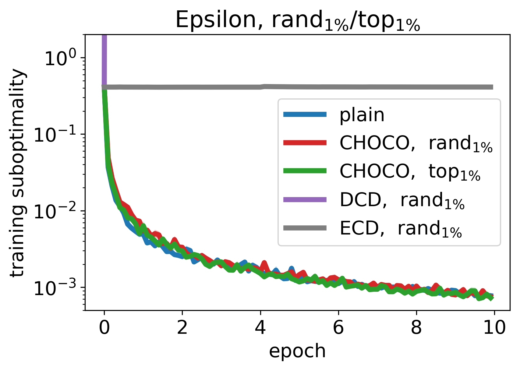
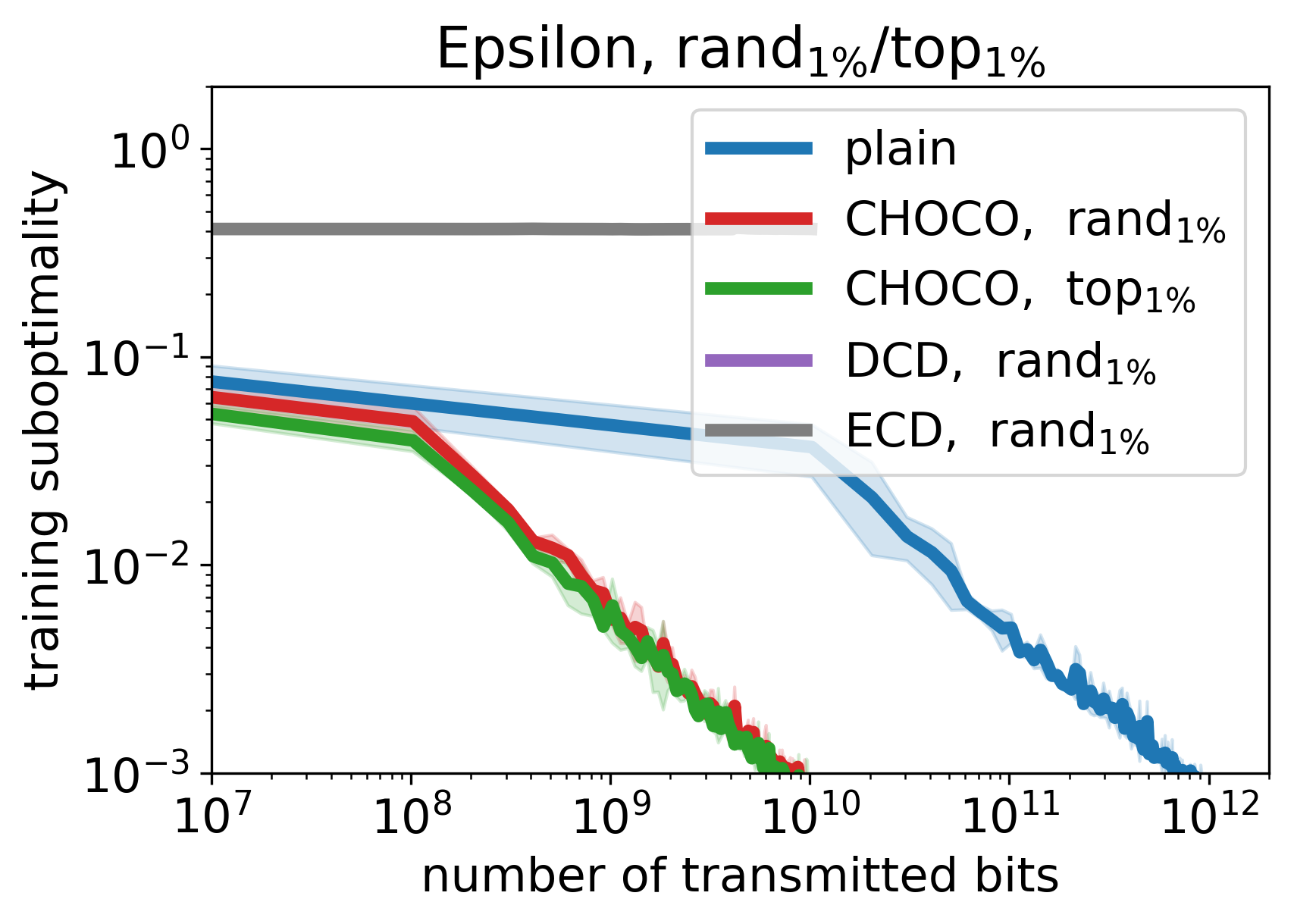
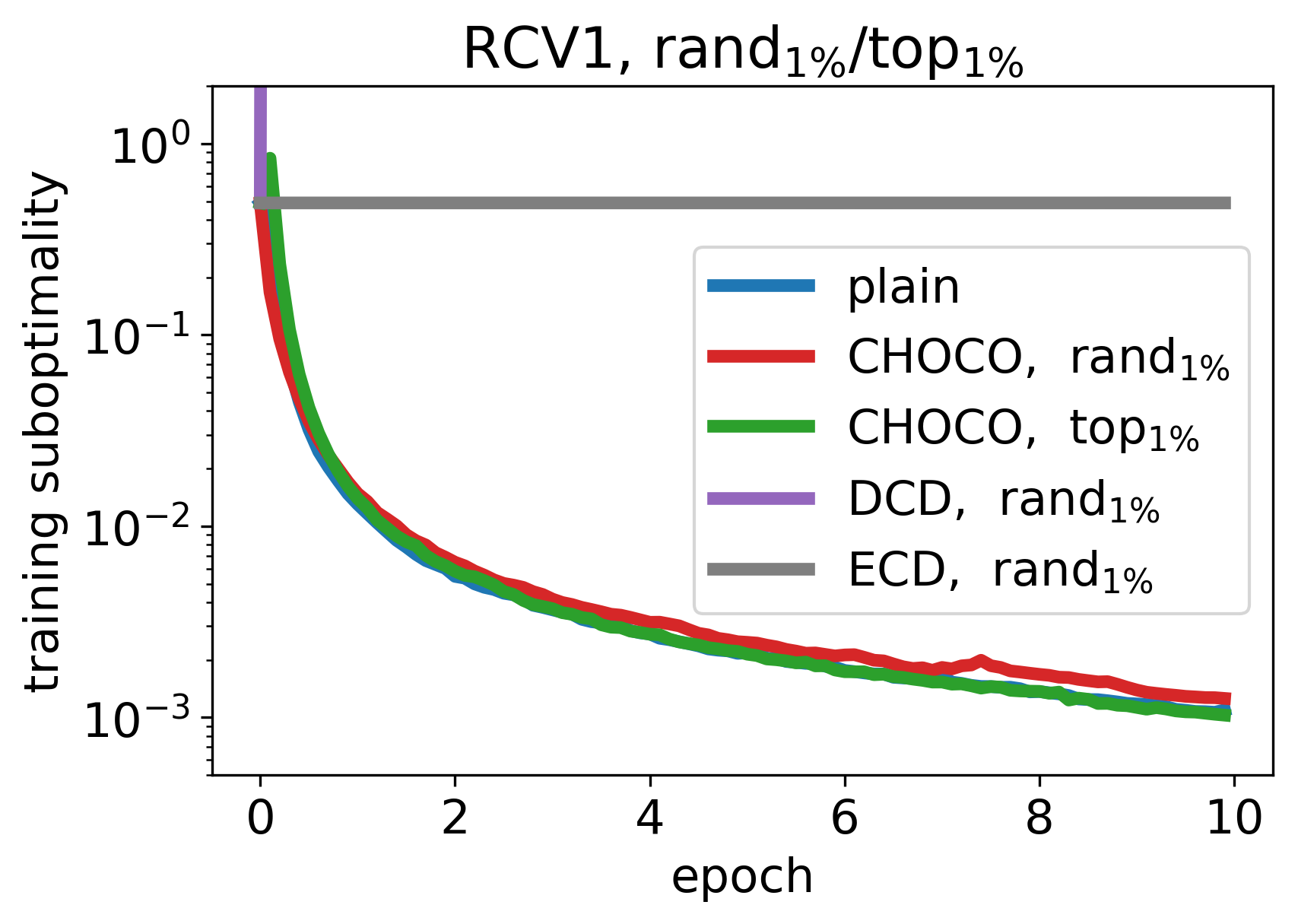
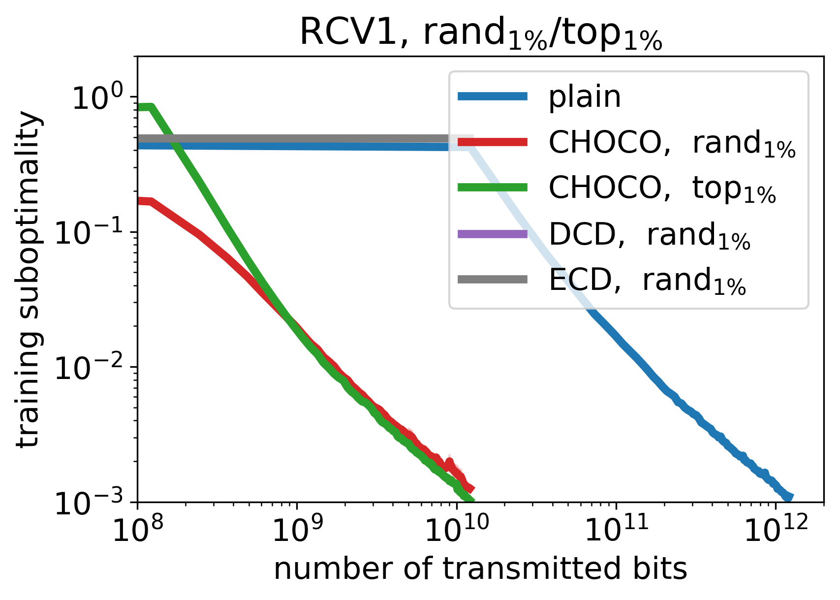
Figure 8: Comparison of Algorithm 3 (plain), ECD-SGD, DCD-SGD and Choco-SGD with ($\operatorname{rand}_{1\%}$) sparsification (in addition ($\operatorname{top}_{1\%}$) for Choco-SGD), for $epsilon$ (top) and $rcv1$ (bottom) in terms of iterations (left) and communication cost (right). Randomly shuffled data between workers.

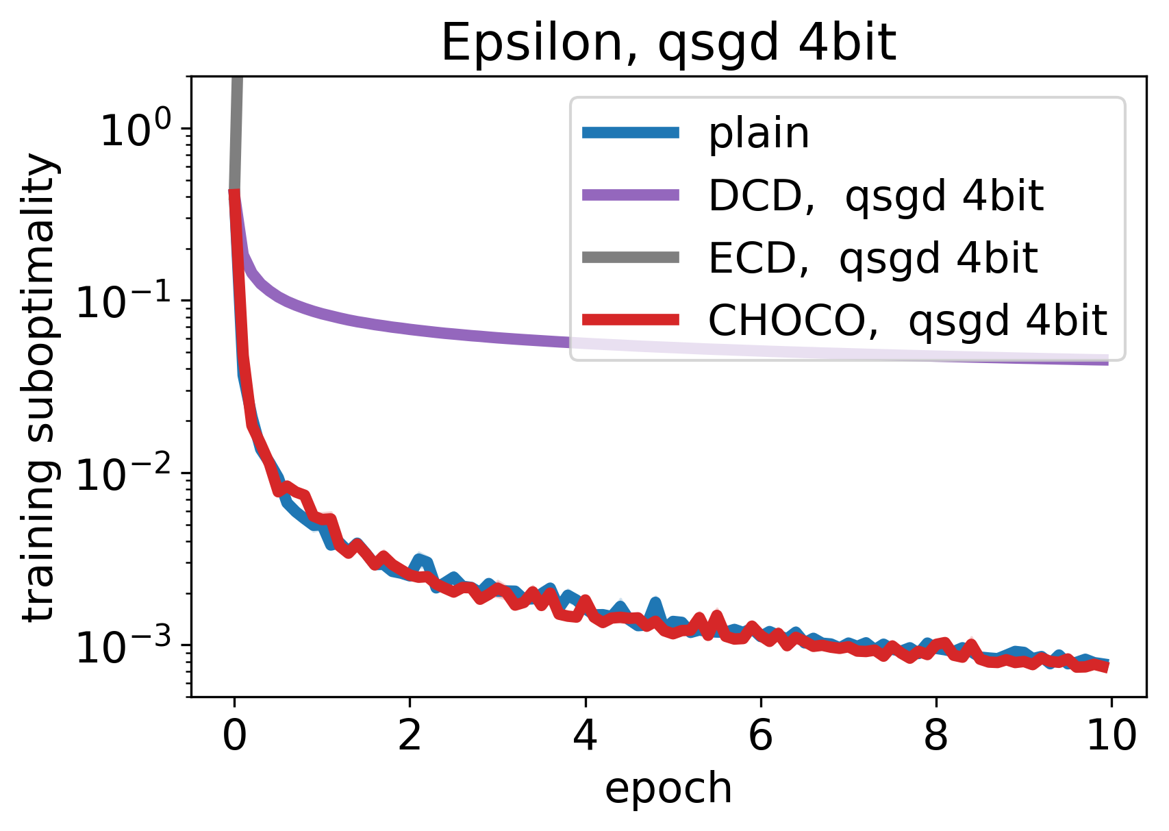
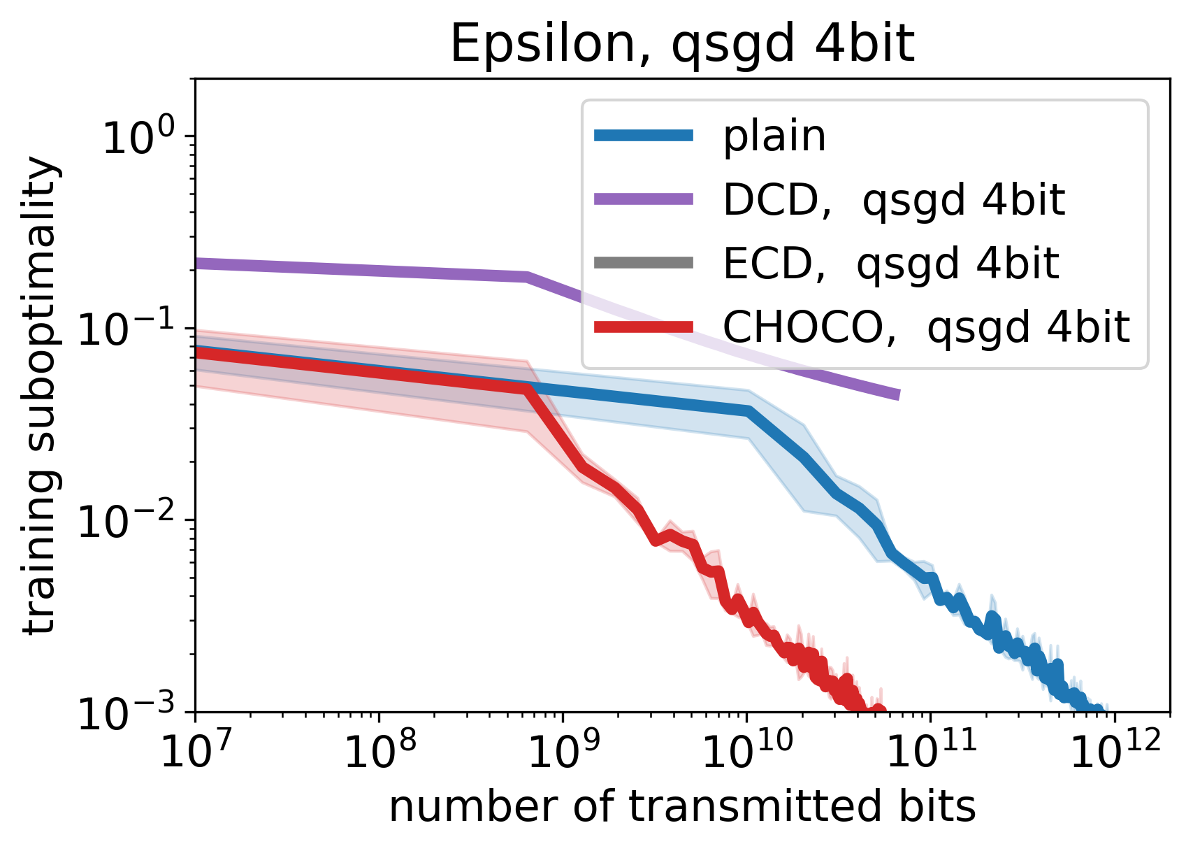
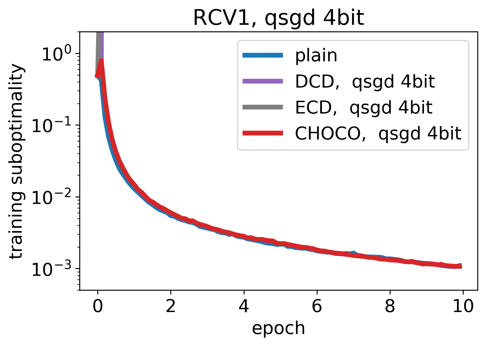
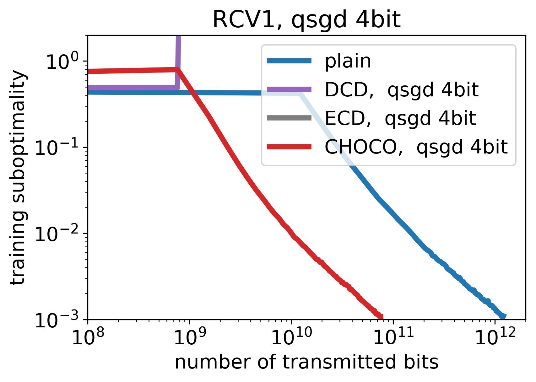
Figure 9: Comparison of Algorithm 3 (plain), ECD-SGD, DCD-SGD and Choco-SGD with ($\operatorname{qsgd}_{16}$) quantization, for $epsilon$ (top) and $rcv1$ (bottom) in terms of iterations (left) and communication cost (right). Randomly shuffled data between workers.

References

• Aldous & Fill (2002) Aldous, D. and Fill, J. A. Reversible markov chains and random walks on graphs, 2002. Unfinished monograph, recompiled 2014, available at http://www.stat.berkeley.edu/$$aldous/RWG/book.html.
• Alistarh et al. (2017) Alistarh, D., Grubic, D., Li, J., Tomioka, R., and Vojnovic, M. QSGD: Communication-efficient SGD via gradient quantization and encoding. In Guyon, I., Luxburg, U. V., Bengio, S., Wallach, H., Fergus, R., Vishwanathan, S., and Garnett, R. (eds.), NIPS - Advances in Neural Information Processing Systems 30, pp.  1709–1720. Curran Associates, Inc., 2017. URL http://papers.nips.cc/paper/6768-qsgd-communication-efficient-sgd-via-gradient-quantization-and-encoding.pdf.
• Alistarh et al. (2018) Alistarh, D., Hoefler, T., Johansson, M., Konstantinov, N., Khirirat, S., and Renggli, C. The convergence of sparsified gradient methods. In Bengio, S., Wallach, H., Larochelle, H., Grauman, K., Cesa-Bianchi, N., and Garnett, R. (eds.), Advances in Neural Information Processing Systems 31, pp.  5977–5987. Curran Associates, Inc., 2018. URL http://papers.nips.cc/paper/7837-the-convergence-of-sparsified-gradient-methods.pdf.
• Assran et al. (2018) Assran, M., Loizou, N., Ballas, N., and Rabbat, M. Stochastic Gradient Push for Distributed Deep Learning. arXiv, November 2018.
• Aysal et al. (2008) Aysal, T. C., Coates, M. J., and Rabbat, M. G. Distributed average consensus with dithered quantization. IEEE Transactions on Signal Processing, 56(10):4905–4918, Oct 2008. ISSN 1053-587X. doi: 10.1109/TSP.2008.927071.
• Bottou (2010) Bottou, L. Large-scale machine learning with stochastic gradient descent. In Lechevallier, Y. and Saporta, G. (eds.), Proceedings of COMPSTAT’2010, pp.  177–186, Heidelberg, 2010. Physica-Verlag HD. ISBN 978-3-7908-2604-3.
• Boyd et al. (2006) Boyd, S., Ghosh, A., Prabhakar, B., and Shah, D. Randomized gossip algorithms. IEEE/ACM Trans. Netw., 14(SI):2508–2530, June 2006. ISSN 1063-6692. doi: 10.1109/TIT.2006.874516. URL https://doi.org/10.1109/TIT.2006.874516.
• Carli et al. (2007) Carli, R., Fagnani, F., Frasca, P., Taylor, T., and Zampieri, S. Average consensus on networks with transmission noise or quantization. In 2007 European Control Conference (ECC), pp.  1852–1857, July 2007. doi: 10.23919/ECC.2007.7068829.
• Carli et al. (2010a) Carli, R., Bullo, F., and Zampieri, S. Quantized average consensus via dynamic coding/decoding schemes. International Journal of Robust and Nonlinear Control, 20:156–175, 2010a. ISSN 1049-8923.
• Carli et al. (2010b) Carli, R., Frasca, P., Fagnani, F., and Zampieri, S. Gossip consensus algorithms via quantized communication. Automatica, 46:70–80, 2010b. ISSN 0005-1098.
• Dekel et al. (2012) Dekel, O., Gilad-Bachrach, R., Shamir, O., and Xiao, L. Optimal distributed online prediction using mini-batches. J. Mach. Learn. Res., 13(1):165–202, January 2012. ISSN 1532-4435. URL http://dl.acm.org/citation.cfm?id=2503308.2188391.
• Duchi et al. (2012) Duchi, J. C., Agarwal, A., and Wainwright, M. J. Dual averaging for distributed optimization: Convergence analysis and network scaling. IEEE Transactions on Automatic Control, 57(3):592–606, March 2012. ISSN 0018-9286. doi: 10.1109/TAC.2011.2161027.
• Fang & Li (2010) Fang, J. and Li, H. Distributed estimation of gauss - markov random fields with one-bit quantized data. IEEE Signal Processing Letters, 17(5):449–452, May 2010. ISSN 1070-9908. doi: 10.1109/LSP.2010.2043157.
• Goodall (1951) Goodall, W. M. Television by pulse code modulation. The Bell System Technical Journal, 30(1):33–49, Jan 1951. ISSN 0005-8580. doi: 10.1002/j.1538-7305.1951.tb01365.x.
• He et al. (2018) He, L., Bian, A., and Jaggi, M. Cola: Decentralized linear learning. In Bengio, S., Wallach, H., Larochelle, H., Grauman, K., Cesa-Bianchi, N., and Garnett, R. (eds.), Advances in Neural Information Processing Systems 31, pp.  4541–4551. Curran Associates, Inc., 2018. URL http://papers.nips.cc/paper/7705-cola-decentralized-linear-learning.pdf.
• Iutzeler et al. (2013) Iutzeler, F., Bianchi, P., Ciblat, P., and Hachem, W. Asynchronous distributed optimization using a randomized alternating direction method of multipliers. In Proceedings of the 52nd IEEE Conference on Decision and Control, CDC 2013, December 10-13, 2013, Firenze, Italy, pp.  3671–3676. IEEE, 2013. doi: 10.1109/CDC.2013.6760448. URL https://doi.org/10.1109/CDC.2013.6760448.
• Jakovetić et al. (2014) Jakovetić, D., Xavier, J., and Moura, J. M. F. Fast distributed gradient methods. IEEE Transactions on Automatic Control, 59(5):1131–1146, May 2014. ISSN 0018-9286. doi: 10.1109/TAC.2014.2298712.
• Johansson et al. (2010) Johansson, B., Rabi, M., and Johansson, M. A randomized incremental subgradient method for distributed optimization in networked systems. SIAM Journal on Optimization, 20(3):1157–1170, 2010. doi: 10.1137/08073038X. URL https://doi.org/10.1137/08073038X.
• Kempe et al. (2003) Kempe, D., Dobra, A., and Gehrke, J. Gossip-based computation of aggregate information. In Proceedings of the 44th Annual IEEE Symposium on Foundations of Computer Science, FOCS ’03, pp.  482–, Washington, DC, USA, 2003. IEEE Computer Society. ISBN 0-7695-2040-5. URL http://dl.acm.org/citation.cfm?id=946243.946317.
• Konecny & Richtárik (2018) Konecny, J. and Richtárik, P. Randomized Distributed Mean Estimation: Accuracy vs. Communication. Frontiers in Applied Mathematics and Statistics, 4:1502, December 2018.
• Lan et al. (2018) Lan, G., Lee, S., and Zhou, Y. Communication-efficient algorithms for decentralized and stochastic optimization. Mathematical Programming, Dec 2018. ISSN 1436-4646. doi: 10.1007/s10107-018-1355-4. URL https://doi.org/10.1007/s10107-018-1355-4.
• Lewis et al. (2004) Lewis, D. D., Yang, Y., Rose, T. G., and Li, F. Rcv1: A new benchmark collection for text categorization research. J. Mach. Learn. Res., 5:361–397, December 2004. ISSN 1532-4435. URL http://dl.acm.org/citation.cfm?id=1005332.1005345.
• Li et al. (2011) Li, T., Fu, M., Xie, L., and Zhang, J. Distributed consensus with limited communication data rate. IEEE Transactions on Automatic Control, 56(2):279–292, Feb 2011. ISSN 0018-9286. doi: 10.1109/TAC.2010.2052384.
• Lian et al. (2017) Lian, X., Zhang, C., Zhang, H., Hsieh, C.-J., Zhang, W., and Liu, J. Can decentralized algorithms outperform centralized algorithms? a case study for decentralized parallel stochastic gradient descent. In Guyon, I., Luxburg, U. V., Bengio, S., Wallach, H., Fergus, R., Vishwanathan, S., and Garnett, R. (eds.), Advances in Neural Information Processing Systems 30, pp.  5330–5340. Curran Associates, Inc., 2017. URL http://papers.nips.cc/paper/7117-can-decentralized-algorithms-outperform-centralized-algorithms-a-case-study-for-decentralized-parallel-stochastic-gradient-descent.pdf.
• Lin et al. (2018) Lin, Y., Han, S., Mao, H., Wang, Y., and Dally, B. Deep gradient compression: Reducing the communication bandwidth for distributed training. In ICLR 2018 - International Conference on Learning Representations, 2018. URL https://openreview.net/forum?id=SkhQHMW0W.
• Nedić & Ozdaglar (2009) Nedić, A. and Ozdaglar, A. Distributed subgradient methods for multi-agent optimization. IEEE Transactions on Automatic Control, 54(1):48–61, Jan 2009. ISSN 0018-9286. doi: 10.1109/TAC.2008.2009515.
• Nedić et al. (2008) Nedić, A., Olshevsky, A., Ozdaglar, A., and Tsitsiklis, J. N. Distributed subgradient methods and quantization effects. In Proceedings of the 47th IEEE Conference on Decision and Control, CDC 2008, pp.  4177–4184, 2008. ISBN 9781424431243. doi: 10.1109/CDC.2008.4738860.
• Nedić et al. (2015) Nedić, A., Lee, S., and Raginsky, M. Decentralized online optimization with global objectives and local communication. In 2015 American Control Conference (ACC), pp.  4497–4503, July 2015. doi: 10.1109/ACC.2015.7172037.
• Olfati-Saber & Murray (2004) Olfati-Saber, R. and Murray, R. M. Consensus problems in networks of agents with switching topology and time-delays. IEEE Transactions on Automatic Control, 49(9):1520–1533, Sep. 2004. ISSN 0018-9286. doi: 10.1109/TAC.2004.834113.
• Pedregosa et al. (2011) Pedregosa, F., Varoquaux, G., Gramfort, A., Michel, V., Thirion, B., Grisel, O., Blondel, M., Prettenhofer, P., Weiss, R., Dubourg, V., Vanderplas, J., Passos, A., Cournapeau, D., Brucher, M., Perrot, M., and Duchesnay, E. Scikit-learn: Machine learning in Python. Journal of Machine Learning Research, 12:2825–2830, 2011.
• Rabbat (2015) Rabbat, M. Multi-agent mirror descent for decentralized stochastic optimization. In 2015 IEEE 6th International Workshop on Computational Advances in Multi-Sensor Adaptive Processing (CAMSAP), pp.  517–520, Dec 2015. doi: 10.1109/CAMSAP.2015.7383850.
• Rakhlin et al. (2012) Rakhlin, A., Shamir, O., and Sridharan, K. Making gradient descent optimal for strongly convex stochastic optimization. In Proceedings of the 29th International Coference on International Conference on Machine Learning, ICML’12, pp.  1571–1578, USA, 2012. Omnipress. ISBN 978-1-4503-1285-1. URL http://dl.acm.org/citation.cfm?id=3042573.3042774.
• Robbins & Monro (1951) Robbins, H. and Monro, S. A Stochastic Approximation Method. The Annals of Mathematical Statistics, 22(3):400–407, September 1951.
• Roberts (1962) Roberts, L. Picture coding using pseudo-random noise. IRE Transactions on Information Theory, 8(2):145–154, February 1962. ISSN 0096-1000. doi: 10.1109/TIT.1962.1057702.
• Scaman et al. (2017) Scaman, K., Bach, F., Bubeck, S., Lee, Y. T., and Massoulié, L. Optimal algorithms for smooth and strongly convex distributed optimization in networks. In Precup, D. and Teh, Y. W. (eds.), Proceedings of the 34th International Conference on Machine Learning, volume 70 of Proceedings of Machine Learning Research, pp.  3027–3036, International Convention Centre, Sydney, Australia, 06–11 Aug 2017. PMLR. URL http://proceedings.mlr.press/v70/scaman17a.html.
• Scaman et al. (2018) Scaman, K., Bach, F., Bubeck, S., Massoulié, L., and Lee, Y. T. Optimal algorithms for non-smooth distributed optimization in networks. In Bengio, S., Wallach, H., Larochelle, H., Grauman, K., Cesa-Bianchi, N., and Garnett, R. (eds.), Advances in Neural Information Processing Systems 31, pp.  2745–2754. Curran Associates, Inc., 2018. URL http://papers.nips.cc/paper/7539-optimal-algorithms-for-non-smooth-distributed-optimization-in-networks.pdf.
• Seide et al. (2014) Seide, F., Fu, H., Droppo, J., Li, G., and Yu, D. 1-bit stochastic gradient descent and its application to data-parallel distributed training of speech DNNs. In Li, H., Meng, H. M., Ma, B., Chng, E., and Xie, L. (eds.), INTERSPEECH, pp.  1058–1062. ISCA, 2014. URL http://dblp.uni-trier.de/db/conf/interspeech/interspeech2014.html#SeideFDLY14.
• Shamir & Srebro (2014) Shamir, O. and Srebro, N. Distributed stochastic optimization and learning. 2014 52nd Annual Allerton Conference on Communication, Control, and Computing (Allerton), pp.  850–857, 2014.
• Sirb & Ye (2016) Sirb, B. and Ye, X. Consensus optimization with delayed and stochastic gradients on decentralized networks. In 2016 IEEE International Conference on Big Data (Big Data), pp.  76–85, Dec 2016. doi: 10.1109/BigData.2016.7840591.
• Sonnenburg et al. (2008) Sonnenburg, S., Franc, V., Yom-Tov, E., and Sebag, M. Pascal large scale learning challenge. 25th International Conference on Machine Learning (ICML2008) Workshop. J. Mach. Learn. Res, 10:1937–1953, 01 2008.
• Stich (2018) Stich, S. U. Local SGD Converges Fast and Communicates Little. arXiv e-prints, art. arXiv:1805.09767, May 2018.
• Stich et al. (2018) Stich, S. U., Cordonnier, J.-B., and Jaggi, M. Sparsified SGD with memory. In Bengio, S., Wallach, H., Larochelle, H., Grauman, K., Cesa-Bianchi, N., and Garnett, R. (eds.), Advances in Neural Information Processing Systems 31, pp.  4452–4463. Curran Associates, Inc., 2018. URL http://papers.nips.cc/paper/7697-sparsified-sgd-with-memory.pdf.
• Tang et al. (2018a) Tang, H., Gan, S., Zhang, C., Zhang, T., and Liu, J. Communication compression for decentralized training. In Bengio, S., Wallach, H., Larochelle, H., Grauman, K., Cesa-Bianchi, N., and Garnett, R. (eds.), Advances in Neural Information Processing Systems 31, pp.  7663–7673. Curran Associates, Inc., 2018a. URL http://papers.nips.cc/paper/7992-communication-compression-for-decentralized-training.pdf.
• Tang et al. (2018b) Tang, H., Lian, X., Yan, M., Zhang, C., and Liu, J. $d^{2}$: Decentralized training over decentralized data. In Dy, J. and Krause, A. (eds.), Proceedings of the 35th International Conference on Machine Learning, volume 80 of Proceedings of Machine Learning Research, pp.  4848–4856, Stockholmsmässan, Stockholm Sweden, 10–15 Jul 2018b. PMLR. URL http://proceedings.mlr.press/v80/tang18a.html.
• Thanou et al. (2013) Thanou, D., Kokiopoulou, E., Pu, Y., and Frossard, P. Distributed average consensus with quantization refinement. IEEE Transactions on Signal Processing, 61(1):194–205, Jan 2013. ISSN 1053-587X. doi: 10.1109/TSP.2012.2223692.
• Tsitsiklis (1984) Tsitsiklis, J. N. Problems in decentralized decision making and computation. PhD thesis, Massachusetts Institute of Technology, 1984.
• Uribe et al. (2018) Uribe, C. A., Lee, S., and Gasnikov, A. A Dual Approach for Optimal Algorithms in Distributed Optimization over Networks. arXiv, September 2018.
• Wangni et al. (2018) Wangni, J., Wang, J., Liu, J., and Zhang, T. Gradient sparsification for communication-efficient distributed optimization. In Bengio, S., Wallach, H., Larochelle, H., Grauman, K., Cesa-Bianchi, N., and Garnett, R. (eds.), Advances in Neural Information Processing Systems 31, pp.  1306–1316. Curran Associates, Inc., 2018. URL http://papers.nips.cc/paper/7405-gradient-sparsification-for-communication-efficient-distributed-optimization.pdf.
• Wei & Ozdaglar (2012) Wei, E. and Ozdaglar, A. Distributed alternating direction method of multipliers. In 2012 IEEE 51st IEEE Conference on Decision and Control (CDC), pp.  5445–5450, Dec 2012. doi: 10.1109/CDC.2012.6425904.
• Wen et al. (2017) Wen, W., Xu, C., Yan, F., Wu, C., Wang, Y., Chen, Y., and Li, H. Terngrad: Ternary gradients to reduce communication in distributed deep learning. In Guyon, I., Luxburg, U. V., Bengio, S., Wallach, H., Fergus, R., Vishwanathan, S., and Garnett, R. (eds.), NIPS - Advances in Neural Information Processing Systems 30, pp.  1509–1519. Curran Associates, Inc., 2017. URL http://papers.nips.cc/paper/6749-terngrad-ternary-gradients-to-reduce-communication-in-distributed-deep-learning.pdf.
• Xiao & Boyd (2004) Xiao, L. and Boyd, S. Fast linear iterations for distributed averaging. Systems & Control Letters, 53(1):65–78, 2004. ISSN 0167-6911. doi: https://doi.org/10.1016/j.sysconle.2004.02.022. URL http://www.sciencedirect.com/science/article/pii/S0167691104000398.
• Xiao et al. (2005) Xiao, L., Boyd, S., and Lall, S. A scheme for robust distributed sensor fusion based on average consensus. In IPSN 2005. Fourth International Symposium on Information Processing in Sensor Networks, 2005., pp.  63–70, April 2005. doi: 10.1109/IPSN.2005.1440896.
• Yuan et al. (2012) Yuan, D., Xu, S., Zhao, H., and Rong, L. Distributed dual averaging method for multi-agent optimization with quantized communication. Systems & Control Letters, 61(11):1053 – 1061, 2012. ISSN 0167-6911. doi: https://doi.org/10.1016/j.sysconle.2012.06.004. URL http://www.sciencedirect.com/science/article/pii/S0167691112001193.
• Zhang et al. (2017) Zhang, H., Li, J., Kara, K., Alistarh, D., Liu, J., and Zhang, C. ZipML: Training linear models with end-to-end low precision, and a little bit of deep learning. In Precup, D. and Teh, Y. W. (eds.), Proceedings of the 34th International Conference on Machine Learning, volume 70 of Proceedings of Machine Learning Research, pp.  4035–4043, International Convention Centre, Sydney, Australia, 06–11 Aug 2017. PMLR. URL http://proceedings.mlr.press/v70/zhang17e.html.