Spatial inhomogeneities in the sedimentation of biogenic particles in ocean flows: analysis in the Benguela region

Abstract

Sedimentation of particles in the ocean leads to inhomogeneous horizontal distributions at depth, even if the release process is homogeneous. We study this phenomenon considering a horizontal sheet of sinking particles immersed in an oceanic flow, and determine how the particles are distributed when they sediment on the seabed (or are collected at a given depth). The study is performed from a Lagrangian viewpoint attending to the properties of the oceanic flow and the physical characteristics (size and density) of typical biogenic sinking particles. Two main processes determine the distribution, the stretching of the sheet caused by the flow and its projection on the surface where particles accumulate. These mechanisms are checked, besides an analysis of their relative importance to produce inhomogeneities, with numerical experiments in the Benguela region. Faster (heavier or larger) sinking particles distribute more homogeneously than slower ones.

JGR-Oceans

IFISC, Instituto de Física Interdisciplinar y Sistemas Complejos (CSIC-UIB), Campus Universitat de les Illes Balears, E-07122 Palma de Mallorca, Spain MTA-ELTE Theoretical Physics Research Group, Pázmany Péter sétany 1/A, H-1117 Budapest, Hungary

C. Lópezclopez@ifisc.uib-csic.es

1 Introduction

The sinking of biogenic particles in the oceans provides the essential food source for the deep-sea organisms, but it is also a fundamental ingredient of the biological carbon pump (Sabine ., 2004). These biogenic particles mainly consist of single phytoplankton cells, aggregates or marine snow, and zooplankton fecal pellets (Turner, 2002).

During the gravitational settling of marine organisms, biochemical reactions occur that modify the fluxes of sinking particles (Nagata ., 2000). Remineralization and grazing decrease the flux of marine snow with depth (Rocha  Passow, 2007). Furthermore, oceanic currents induce lateral transport of sinking particles due to the relatively small vertical velocity compared to horizontal ocean velocities. This implies that sinking particles travel almost horizontally, and their source area may be rather distant from the location where they sediment in the deep ocean (Siegel  Deuser, 1997; Waniek ., 2000; van Sebille ., 2015; Liu ., 2018). When settled on the seafloor or collected at a given depth by sediment traps (Buesseler ., 2007), a relevant feature is the presence of inhomogeneities in the spatial distribution of the particles, i.e. collecting sites that are relatively close can receive a significantly different amount of particles (Liu ., 2018). An important contributing factor is the presence of inhomogeneities already in the production of particles in the upper ocean (Giering ., 2018). Also, resuspension mechanisms near the ocean floor (Diercks ., 2018) and the combined effect of biochemical reactions and ocean currents acting while the particles are sinking (Deuser ., 1990) contribute to the mentioned feature.

Concerning some of these processes relevant on non-geological time scales, much has been learned by suspending sediment traps to collect the particles: for example, about the amount of particles delivered from the surface, the organisms that are involved, their size and thus their settling speed, the aggregates that form while sinking (marine snow), and the importance of the inhomogeneities in the initial distribution at the surface (Giering ., 2018). But many questions still remain open referring to the above-mentioned inhomogeneities in the final distribution of the particles: How do the spatial patterns of sedimentation depend on the characteristics of the particles? How do oceanic currents shape these patterns? How do the biogeochemical processes shape them during sinking? What is the relative importance of the different mechanisms involved? Proper answers to these questions will for sure be relevant for a proper quantification of the biological carbon pump, and help identify those areas of the oceans that can be labeled as sinks or sources of carbon.

This paper focuses on the role of transport processes in some of the above questions. In particular, on how a layer of particles homogeneously released at the surface would give rise to spatial inhomogeneities when arriving to some depth, because of the stretching and folding action of the oceanic currents during the sinking process. We do not consider geological time scales, so that our results explicitly attempt to provide a basis for explaining some features of measurements carried out with sediment traps (Liu ., 2018). We will illustrate that the basic feature, the presence of strong spatial gradients, appears even when starting from an initially homogenous distribution under the sole action of oceanic turbulence. As a consequence, besides initial horizontal gradients in the production of the particles (Giering ., 2018), transport processes might also provide with an equally important contribution to the final inhomogeneities.

We perform numerical experiments in the Benguela region (at the southwestern coasts of Africa) by letting particles sink from a homogeneous layer near the marine surface and then observing where they arrive at a given depth. We then analyze the accumulated density of particles at different locations to learn about the effect of transport by the ocean flow. Since we focus on the effect of transport, disregarding any other factor such as production inhomogeneities or particle degradation, our study is of qualitative nature, without the aim of a quantitative interpretation of particular observational data.

In Drótos . (2019) we found analytical expressions for the ratio between the density of particles accumulated on a horizontal surface at a given depth and the original density. These expressions are cast in terms of the trajectories of the particles and the properties of the velocity field along these trajectories. In this paper we apply this framework to the sinking of biogenic particles in the Benguela region, using a velocity field of an ocean model simulation of this region. Since the vertical motion of the particles involves a settling term which depends on the particles’ density and size, the final distribution will also depend on these physical characteristics. Thus, we can compare the inhomogeneities in the distributions formed by particles of different densities and sizes by studying different values of the settling velocity.

A main finding in Drótos . (2019) was that the dependence of the above-mentioned factor (determining the particle density on the horizontal collecting surface) can be understood in terms of two basic processes: the stretching of the sinking sheet of particles, and the projection of this sheet on the surface where particles accumulate. In our numerical experiments in Benguela we check the validity of these analytic expressions, analyze how they describe the inhomogeneities in sedimentation in this particular geographical zone, show that inhomogeneities may indeed be rather strong, and test the relative importance of the two mechanisms, stretching and projection, that produce inhomogeneity. Also, we will examine the role of the resolution at which the distribution on the accumulating surface is sampled, and provide new analytical formulae that help the discussion of the results in the oceanic framework. The computations in this paper assume a homogeneous but infinitely thin horizontal initial particle layer. Thus, these results are aimed to illustrate (i) that the sole action of transport in realistic ocean flows is able to introduce strong inhomogeneities under appropriate circumstances, and (ii) some relevant properties of this process.

The paper is organized as follows: In section 2 we present the data and the methods of our work, which includes the analytical formulae describing the accumulated density of particles at a given depth, the decomposition of the process into stretching and projection, and also the statistical methodology to compare these results with the ones obtained from direct sampling of particle positions. In section 3 we present our numerical results for the Benguela region. We show spatial sedimentation patterns for different types of particles and compare these with the analytical results, identifying the dominant mechanisms for the generation of inhomogeneities. In section 4 we discuss some of the results, and in section 5 we present a summary and conclusions.

2 Data and methods

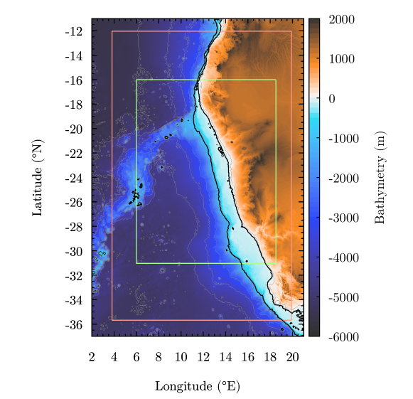
Figure 1: Map of the region of study. Coloring corresponds to bathymetry. The oceanic part of the red rectangle is the region used for simulations of the ROMS model. The oceanic part of the green rectangle is the region for the numerical experiments. Black lines represent $100$ and $1000\mathrm{m}$ depth, i.e., the particle releasing depth and the accumulation depth, respectively.

A three-dimensional model is used to simulate the vertical transport of biogenic particles produced in the euphotic zone and sedimenting to the deep sea. It is composed of the output velocity field of a hydrodynamical model combined with a Lagrangian particle tracking model. We next specify the area of study (the Benguela region), the velocity data, and the Lagrangian equations for the sinking dynamics.

2.1 Area of study and velocity data

The velocity data used is the output of a regional ocean model (Regional Ocean Modelling System, ROMS) simulation of the Benguela region (Figure 1). This hydrostatic, free-surface, primitive-equations hydrodynamical model was forced with climatological data. The area of the data set extends from $12^{\circ}$ to $35^{\circ}S$ and from $4^{\circ}$ to $19^{\circ}E$ (red rectangle in Figure 1). The velocity field ($\mathbf{u}=(u_{x},u_{y},u_{z})$) consists of two years of daily averaged zonal ($u_{x}$), meridional ($u_{y}$), and vertical ($u_{z}$) components, stored in a three-dimensional grid with a horizontal resolution of $1/12^{\circ}$ and $32$ vertical terrain-following levels. Additional details on the model configuration can be found in Gutknecht . (2013).

2.2 Lagrangian description of sinking particles

We are interested in describing the sinking dynamics of particulate organic matter biologically generated close to the ocean surface, in the euphotic layer. Sizes of these particles or aggregates range between 1$\mu$m and more than 1 cm, and densities are between 1050 and 2700 kg/m³ (Monroy ., 2017). For sizes smaller than 200 $\mu$m, i.e. for the majority of particle types except for the largest aggregates and zooplankton bodies (meso- and macro-zooplankton), particle inertia can be safely neglected (Monroy ., 2017) and the velocity of the particle, $\mathbf{v}$, is well approximated by the sum of the velocity field of the fluid $\mathbf{u}$ and a vertical settling velocity $\mathbf{v}_{\mathrm{s}}$ (Monroy ., 2017; Drótos ., 2019). This last quantity is the terminal velocity for sinking in a quiescent fluid, pointing vertically downwards. It depends on the physical properties of the particles as

$$\mathbf{v}_{\mathrm{s}}=(1-\beta)\mathbf{g}\frac{a^{2}}{3\beta\nu},\quad\textrm{with}\quad\beta=\frac{3\rho_{\mathrm{f}}}{2\rho_{\mathrm{p}}+\rho_{\mathrm{f}}},$$ (1)

where $a$ is the particle radius (particles are assumed to be spherical), $\mathbf{g}$ is the gravitational acceleration, $\rho_{\mathrm{f}}$ is the fluid density, $\rho_{\mathrm{p}}$ is the particle density, and $\nu$ is the kinematic viscosity of the fluid. Values of the modulus of the settling velocity $v_{\mathrm{s}}=|\mathbf{v}_{\mathrm{s}}|$ for the biogenic particles under study are in the range 1mm/day-1km/day, but we will concentrate here on the most common values which are 35-235m/day (Table 1). The vertical fluid velocities in the mesoscale flow field we are considering are of the order of 10m/day at most; we will thus always have a strictly negative vertical velocity for the particles, $v_{z}<0$, i.e. the particles will always be sinking. Constant size and contrast of density between particle and water are assumed for each particle along its downward path. This implies, as mentioned in the introduction, the neglection of biogeochemical and (dis)aggregation processes that may occur: our focus is on the role of transport. As a crude way to estimate the effect of small-scale motions that are unresolved by the hydrodynamical model, we add a white noise term to the particle velocity, with different intensities in the vertical and the horizontal directions. In summary, the model we use for the velocity of the sinking particles is the following stochastic equation (Monroy ., 2017):

$$\frac{d\mathbf{R}}{dt} = \mathbf{v}(\mathbf{R},t),$$

$$\mathbf{v} = \mathbf{u}+\mathbf{v}_{\mathrm{s}}+\mathbf{W}.$$ (2)

$\mathbf{R}=\mathbf{R}(\mathbf{r}_{0},t)$ is the position at time $t$ of the particle that was released at position $\mathbf{r}_{0}$ at the initial time $t_{0}$. $\mathbf{v}_{\mathrm{s}}$ is the settling velocity discussed above, and $\mathbf{W}(t)\equiv 2D_{\mathrm{h}}\mathbf{W}_{\mathrm{h}}(t)+2D_{\mathrm{v}}\mathbf{W}_{z}(t)$, with $(\mathbf{W}_{\mathrm{h}},W_{z})=(W_{x}(t),W_{y}(t),W_{z}(t))$ being a three-dimensional vector Gaussian white noise with zero mean and with correlations $\langle W_{i}(t)W_{j}(t^{\prime})\rangle=\delta_{ij}\delta(t-t^{\prime})$, $i,j=x,y,z$. We consider a horizontal eddy diffusivity, $D_{\mathrm{h}}$, that depends on the resolution length scale $l$ according to the Okubo formula (Okubo, 1971; Sandulescu ., 2006; Hernández-Carrasco ., 2011): $D_{\mathrm{h}}(l)=2.055\times 10^{4}l^{1.55}(\mathrm{m}^{2}\mathrm{s}^{-1})$. Thus, when taking $l\simeq 8\mathrm{km}=8000\mathrm{m}$ (corresponding to $1/12^{\circ}$), we obtain $D_{\mathrm{h}}=40\mathrm{m}^{2}\mathrm{s}^{-1}$. In the vertical direction we use a constant value of $D_{\mathrm{v}}=10^{-5}\mathrm{m}^{2}\mathrm{s}^{-1}$ (Rossi ., 2013). In the derivation of our analytic formulae, however, the particle velocity field is assumed to be a smooth function, which excludes the presence of the irregular noise term. In consequence, the noise term will be chosen to be zero for the evaluation of the geometrical formulae of section 2.4. The results obtained from these formulae will be, however, compared with the histograms obtained from direct sampling of densities from simulated particle trajectories in the presence of the noise term. Thus, differences between the analytical expressions and the computed histograms would give an idea of the relevance of unresolved flow features on the sedimentation process.

Parameter	Values
Settling velocity $v_{\mathrm{s}}$	$35$, $40$, $45$, and then from $50$ to $225\mathrm{m}/\mathrm{day}$ using steps of $25\mathrm{m}/\mathrm{day}$
Coarse-graining radius $R$	from $10\mathrm{km}$ to $100\mathrm{km}$ using steps of $5\mathrm{km}$
Starting depth	$-100\mathrm{m}$
Final depth	$-1000\mathrm{m}$
Integration time step	$6~{}\mathrm{hours}$
Starting date	20 August 2008

Table 1: Parameters used in the sedimentation simulations.

Three-dimensional Lagrangian particle trajectories are obtained by means of numerical integration of equation (2) using a second-order Heun method with absorbing boundary condition (that is, the integration halts if the trajectory escapes the domain of the simulation (red rectangle in Fig. 1) or reaches the seabed outside the domain of the analysis (green rectangle in Fig. 1)). For the numerical integration of the trajectories without noise, a fourth-order Runge–Kutta scheme is used. We select $6$ hours for the integration time step and linear interpolation in time and space to obtain the flow velocity $\mathbf{u}$ at the location of the particle while it moves between ROMS grid points.

2.3 Numerical experiment and direct sampling of the accumulated density

We consider a situation in which particles are released with uniform density from a horizontal layer close to the surface, at an initial time $t_{0}$, and study how the transport process results in an inhomogeneous distribution of particles when they are collected in a deeper layer. More explicitly, on 20 of August 2008 we initialize a large number of particles at a depth $z_{0}=100\mathrm{m}$ equispaced in the zonal and meridional directions, which is conveniently achieved by using a sinusoidal projection (Ser-Giacomi ., 2015). Then each particle of this horizontal layer is evolved by equation (2) until it reaches the depth $z=1000\mathrm{m}$ (or escapes as described earlier). The calculation is repeated using a range of settling velocities (see Table 1). Note that, according to equation (1), increasing the magnitude $v_{\mathrm{s}}$ of the settling velocity means considering heavier particles (or larger ones). The final positions are used to obtain the number $n^{z}_{R}(\mathbf{x})$ of particles that are accumulated within a circular sampling area of radius $R$ around a horizontal position $\mathbf{x}$ at the given depth $z$ (we use the notation $\mathbf{r}=(\mathbf{x},z)$ to distinguish between horizontal, $\mathbf{x}$, and vertical, $z$, components of a three-dimensional vector $\mathbf{r}$). The number density of accumulated particles in this circle is thus $\sigma^{R}_{z}(\mathbf{x})=n^{z}_{R}(\mathbf{x})/(\pi R^{2})$, where the subindex $z$ indicates that we are measuring the accumulated density at a depth $z$. We will describe our results in terms of the density on the collecting surface but this does not need to be an actual physical surface extending over the whole domain of interest, such as the bottom of the sea. For example sediment traps have a rather small collecting surface and are commonly suspended at some intermediate depth. The inhomogeneities we will describe on our virtual collecting surface would apply to differences in number of captured particles between two traps at the same depth but at two distant horizontal positions (Liu ., 2018). We locate the centers $\mathbf{x}$ of our sampling areas on a regular grid in latitude and longitude within the collecting surface, with a spacing of $1/20^{\circ}$ in each direction. The range of the values for the coarse-graining radius $R$ used here is shown in Table 1. These are rather large values, as adequate to discuss large-scale and statistical features of the sedimented density. To address densities sampled by small devices such as sediment traps, smaller values of $R$ need to be used, or rather, to use directly the local geometrical approach discussed in section 2.4. Alternatively, local measurements should be coarse-grained to characterize large-scale structures in the density. As found in Monroy . (2017), and consistently with observations (Liu ., 2018), the accumulated density $\sigma^{R}_{z}(\mathbf{x})$ is horizontally highly inhomogeneous. The main purpose of this paper is to explore some of the mechanisms leading to these inhomogeneities.

To quantify the inhomogeneity of the accumulated density in the final surface, we compute the density factor (Drótos ., 2019), i.e., the density relative to its value at the initial depth, $\sigma_{0}$, i.e.:

$$\mathcal{F}^{R}_{\mathrm{hist}}(\mathbf{x})\equiv\frac{\sigma^{R}_{z}(\mathbf{x})}{\sigma_{0}}=\frac{n^{z}_{R}(\mathbf{x})}{n_{R}^{0}},$$ (3)

where $n_{R}^{0}$ is the number of particles initialized in a circle of radius $R$ in the release layer, which is related to the homogeneous release density $\sigma_{0}$ by $n_{R}^{0}=\sigma_{0}\pi R^{2}$. The subindex ‘hist’ in $\mathcal{F}^{R}_{\mathrm{hist}}$ indicates that this quantity is computed from equation (3) that amounts to computing a histogram, and distinguishes it from the geometric quantity $\mathcal{F}^{R}_{\mathrm{geo}}$ to be defined in the next section. In all our numerical experiments we fix $n_{R}^{0}=1000$ particles, so that the initial density depends on the choice of the sampling circles and is approximately $\sigma_{0}=1000/(\pi R^{2})$. This number of particles proved to be high enough to ensure the numerical independence of $\mathcal{F}^{R}_{\mathrm{hist}}$ with respect to changes in the initial surface density.

Sampling circles near the coastline receive significantly less particles than those in the ocean interior due to the absorbing boundary condition. We avoid this effect by discarding circles for which more than $0.01\%$ of their area is occupied by land. Furthermore, boundary effects are also present in sampling areas close to the model domain borders. We also discard sampling areas close to the borders of the hydrodynamical model, and only keep those whose centers are inside the rectangle $2$ to $18^{\circ}E$ and $31$ to $16^{\circ}S$ (green rectangle in Figure 1).

2.4 Geometrical computation of the accumulated density

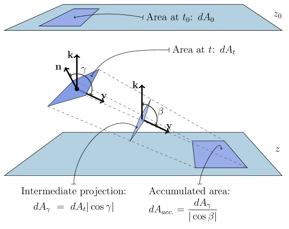
Figure 2: Schematic illustration of infinitesimal areas and angles involved in the geometrical computation of the density factor $\mathcal{F}_{\mathrm{geo}}$. A small patch of particles of area $dA_{0}$, located horizontally at depth $z_{0}$ at time $t_{0}$, is advected by the velocity field $\mathbf{v}$. At time $t$ the area of this patch is $dA_{t}$. The accumulated area is $dA_{\mathrm{acc}}$, which corresponds to its projection parallel to the flow direction $\mathbf{v}$ onto the horizontal plane. $\mathbf{k}$ is the vertical unit vector, and $\mathbf{n}$ is the unit vector normal to the patch at time $t$. Assuming mass conservation, the factors $\mathcal{F}_{\mathrm{geo}}$, $\mathcal{P}$ and $\mathcal{S}$ are given by $\mathcal{F}_{\mathrm{geo}}=\frac{dA_{0}}{dA_{\mathrm{acc}}}$, $\mathcal{S}=\frac{dA_{0}}{dA_{t_{z}}}$ and $\mathcal{P}=\frac{dA_{t_{z}}}{dA_{\mathrm{acc}}}=\left|\frac{\cos\beta}{\cos\gamma}\right|$, where $t_{z}$ is the time of arrival of the infinitesimal area at the final surface at depth $z$.

Following Drótos . (2019) we next introduce a geometrical approach to compute the density factor. For the derivations in this section, and for the later numerical evaluation of the resulting formulae, we use equation (2) without the noise term, i.e., with $D_{\mathrm{h}}=D_{\mathrm{v}}=0$, since our mathematical manipulations are only well-defined for smooth velocity fields.

As illustrated in Figure (2), let us consider the sinking of the initially horizontal particle layer that was at depth $z_{0}$ at time $t_{0}$, and let us focus on the trajectory $\mathbf{R}=\mathbf{R}(\mathbf{r}_{0},t)$ of a particle of the layer, which was at $\mathbf{r}_{0}=(\mathbf{x}_{0},z_{0})$ at time $t_{0}$. Let $dA_{0}$ be the area of an infinitesimal patch in the horizontal release layer around that particle, containing a number of particles $dn_{0}=\sigma_{0}dA_{0}$. (Since we use a large number, we neglect the discrete nature of the particle number and approximate it by a continuous variable.) Under the action of the flow, during the sinking process the area occupied by these particles will expand or shrink, taking values $dA_{t}$, until arriving (non-horizontally in general) to the collecting horizontal surface at depth $z$ (reached at time $t_{z}$), where the particles will leave a horizontal footprint of area $dA_{\mathrm{acc}}$. Since the number of particles is conserved, this will produce an accumulated density $\sigma_{z}=dn_{0}/dA_{\mathrm{acc}}$. We define the geometric density factor $\mathcal{F}_{\mathrm{geo}}$ at the horizontal location $\mathbf{x}$ where the particle that started at $\mathbf{r}_{0}$ reaches the layer at depth $z$ as

$$\mathcal{F}_{\mathrm{geo}}\equiv\frac{\sigma_{z}}{\sigma_{0}}=\frac{dA_{0}}{~{}~{}dA_{\mathrm{acc}}}=\frac{dA_{0}}{~{}dA_{t_{z}}}\frac{dA_{t_{z}}}{~{}dA_{\mathrm{acc}}}\equiv\mathcal{S}~{}\mathcal{P}.$$ (4)

$dA_{t_{z}}$ is the area of the sinking patch at time $t_{z}$ when the focus particle reaches depth $z$. We have introduced, following Drótos . (2019), the stretching factor $\mathcal{S}=dA_{0}/dA_{t_{z}}$ which gives the ratio between the initial area surrounding the focus particle and its value when reaching the collecting surface at depth $z$, and the projection factor $\mathcal{P}=dA_{t_{z}}/dA_{\mathrm{acc}}$. This last quantity is the ratio between this final area of the sinking patch (which in general would be non-horizontal) and its footprint on the horizontal collecting layer. Thus, it gives the geometric projection of the moving patch onto the horizontal accumulation plane parallel to the direction of the flow, see Figure 2. One interest of the decomposition (4) into a stretching and a projection factor is that it allows to identify which are the dominant mechanisms producing the observed inhomogeneities in the sedimentation process under different settings and conditions. We will do so in section 3 for the case of particles sinking in the Benguela zone, giving special interest to the dependence on the settling velocity component of $\mathbf{v}$, which encodes the physical properties of the sinking particles.

A more detailed derivation of equation (4) was given in Drótos . (2019). Also, several expressions for the explicit calculation of $\mathcal{S}$ and $\mathcal{P}$ were given there, of which we select the following ones (see Appendices J and K of Drótos . (2019)) as more convenient for application to the oceanic flow:

$$\mathcal{S}(\mathbf{x}) = \left|\mathbf{\tau}_{x}(t_{z})\times\mathbf{\tau}_{y}(t_{z})\right|^{-1},$$ (5)

$$\mathcal{P}(\mathbf{x}) = \left|\frac{v_{z}}{\mathbf{v}\cdot\mathbf{n}}\right|=\left|\frac{\cos\beta}{\cos\gamma}\right|.$$ (6)

At any time $t$, $\mathbf{\tau}_{x}(t)$ and $\mathbf{\tau}_{y}(t)$ are two vectors tangent to the sinking surface, at the position of the focus particle, calculated as

$$\mathbf{\tau}_{x}(t)=\frac{\partial\mathbf{R}(\mathbf{r}_{0},t)}{\partial x_{0}}\quad,\quad\mathbf{\tau}_{y}(t)=\frac{\partial\mathbf{R}(\mathbf{r}_{0},t)}{\partial y_{0}},$$ (7)

where $x_{0}$ and $y_{0}$ are two orthogonal coordinates on the initial horizontal surface (we use zonal and meridional distances, see Appendices A and B). In terms of these tangent vectors the unit vector $\mathbf{n}$ normal to the sinking surface at time $t$ reads as

$$\mathbf{n}=\frac{\mathbf{\tau}_{x}\times\mathbf{\tau}_{y}}{|\mathbf{\tau}_{x}\times\mathbf{\tau}_{y}|}.$$ (8)

In the expression for the projection factor $\mathcal{P}$, equation (6), the vectors and angles involved are defined in Figure 2, namely

$$v_{z} = v\cos\beta,$$

$$\mathbf{v}\cdot\mathbf{n} = v\cos\gamma,$$ (9)

i.e, $\beta$ is the angle between the vertical direction and the direction of the velocity of the particle at the final time $t_{z}$, and $\gamma$ is the angle between the direction of the particle velocity and the normal to the layer (both at the final time as well). Stretching and projection factors at location $\mathbf{x}$ are evaluated in terms of quantities defined at the final time, $t_{z}$, but they depend on the whole history of the sinking particle through the initial-position derivatives defining $\mathbf{\tau}_{x}$, $\mathbf{\tau}_{y}$, and then $\mathbf{n}$.

Equation (6) is readily derived from the projection geometry in Figure 2. Equation (5) is a standard geometrical result for the ratio between the areas of an evolving infinitesimal surface at two times, but we give a short derivation of it in Appendix A. We also give an alternative expression and derive some simplifications valid in special cases. In Appendix B we also give additional details on the numerical implementation of the computation.

Note that equation (4) associates a change in the density to the infinitesimal neighborhood of every trajectory, so that evaluating equation (4) is already meaningful when following a single particle. Once the velocity field and the initial conditions are fixed, the density factor becomes unique for this trajectory. Furthermore, if we prescribe an initial distribution of particles (as a continuous function of space) then the final density on the entire accumulation level also becomes unique. The inverse relationships, however, are not unique: Measuring the final density does not allow inferring the velocity field. Also, because of the time dependence of the velocity field, correct backtracking of the particles and reconstruction of the initial density are not possible unless the deposition time for each particle is known. As a practical consequence, the catchment area cannot be uniquely identified just from sedimentation data.

2.5 Statistical analysis: relating direct sampling to the geometrical computation

Since the geometrical computation (section 2.4) gives the estimation of the density factor for an infinitesimal sampling area instead of a finite one of radius $R$ as the direct sampling method of section 2.3 does, we can compare the results only in the limit of zero sampling area, $\mathcal{F}_{\mathrm{geo}}=\mathcal{F}^{R\to 0}_{\mathrm{hist}}$. Estimating this limit is, however, unfeasible due to the finite number of particles used in the numerical implementation. Instead, we perform a coarse graining of the geometrical results using the same circular sampling areas as in the direct sampling method. The coarse-grained value, referring to a circle of radius $R$ around a location $\mathbf{x}$, of the density factor is computed by taking the harmonic mean of the geometrical density factors at the final locations $\mathbf{x}_{i}$ of particle trajectories that end inside the sampling area of radius $R$ centered at $\mathbf{x}$:

$$\mathcal{F}^{R}_{\mathrm{geo}}(\mathbf{x})=\frac{n_{R}(\mathbf{x})}{\sum_{i=1}^{n_{R}(\mathbf{x})}\frac{1}{\mathcal{F}_{\mathrm{geo}}(\mathbf{x}_{i})}},$$ (10)

where $n_{R}(\mathbf{x})$ is the number of such trajectories. A simple arithmetic mean of the density factors is not appropriate since it will be biased towards high values: there will be more particles falling in regions of high density. See Appendix C for why harmonic mean is the correct choice.

Similarly, we compute the coarse-grained version of stretching and projection factors by

$$\mathcal{S}^{R}(\mathbf{x})\simeq\frac{n_{R}(\mathbf{x})}{\sum_{i=1}^{n_{R}(\mathbf{x})}\frac{1}{\mathcal{S}(\mathbf{x}_{i})}}\quad\text{and}\quad\mathcal{P}^{R}(\mathbf{x})\simeq\frac{n_{R}(\mathbf{x})}{\sum_{i=1}^{n_{R}(\mathbf{x})}\frac{1}{\mathcal{P}(\mathbf{x}_{i})}},$$ (11)

respectively. The coarse-grained version of the density factor $\mathcal{F}^{R}_{\mathrm{geo}}$ is certainly not the product of the coarse-grained versions of stretching and projection as given by equations (11), but we use these last expressions as a qualitative estimation of the proportion of inhomogeneities arising from each of the two mechanisms.

We will compare the value of $\mathcal{F}^{R}_{\mathrm{geo}}(\mathbf{x})$ obtained from (10) with the value of $\mathcal{F}^{R}_{\mathrm{hist}}(\mathbf{x})$ obtained from equation (3) in the same configuration, for which we place the sampling areas of radius $R$ at the same locations (i.e. in a grid of spacing $1/20^{\circ}$ in latitude and longitude).

$\mathcal{F}_{\mathrm{geo}}$ (as well as $\mathcal{S}$, $\mathcal{P}$ and $\sigma_{z}$) is a property of each point $\mathbf{x}$ on the collecting surface, in contrast with $\mathcal{F}^{R}_{\mathrm{hist}}$ which is a property of a neighborhood of radius $R$ around each point. But both characterize the same density inhomogeneities at the collecting surface and they should coincide after properly averaging (or coarse-graining) $\mathcal{F}_{\mathrm{geo}}$ in the same neighborhood of radius $R$, as described in the previous paragraph. Any remaining difference between the two quantities could only arise because the noise term, modeling small scales unresolved by the ROMS simulation, is included in the integration of the particle trajectories when computing $\mathcal{F}^{R}_{\mathrm{hist}}$, but not when computing $\mathcal{F}^{R}_{\mathrm{geo}}$. Consequently, the latter computation captures only the inhomogeneities due to the mesoscales in the ocean flow, which are the resolved scales of the hydrodynamical model. Comparing such results with $\mathcal{F}^{R}_{\mathrm{hist}}$ computed from noisy trajectories allows us to check how robust the mesoscale phenomena are with respect to the addition of velocity components not included there, such as the noise term in (2).

A quantitative comparison of $\mathcal{F}^{R}_{\mathrm{geo}}$ with $\mathcal{F}^{R}_{\mathrm{hist}}$ is done via the Pearson correlation coefficient:

$$\rho(\mathcal{F}^{R}_{\mathrm{hist}},\mathcal{F}^{R}_{\mathrm{geo}})=\frac{\mathrm{Cov}(\mathcal{F}^{R}_{\mathrm{hist}},\mathcal{F}^{R}_{\mathrm{geo}})}{\sigma_{\mathcal{F}^{R}_{\mathrm{hist}}}\sigma_{\mathcal{F}^{R}_{\mathrm{geo}}}},$$ (12)

where $\sigma_{\mathcal{F}^{R}_{\mathrm{hist}}}$ and $\sigma_{\mathcal{F}^{R}_{\mathrm{geo}}}$ are the respective standard deviations. The averages are taken with respect to all the sampling points $\mathbf{x}$ used. We analogously apply the Pearson correlation coefficient to characterize the density factor’s similarity with stretching and projection factors as well.

3 Numerical results

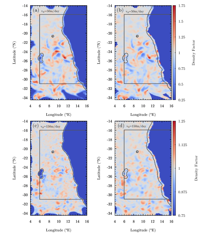
Figure 3: The density factor computed via direct sampling, $\mathcal{F}^{R}_{\mathrm{hist}}$ from equation (3), panels (a) and (c); and via the geometrical approach, $\mathcal{F}^{R}_{\mathrm{geo}}$ from equation (10), panels (b) and (d)). Two different settling velocities, $50\mathrm{m}/\mathrm{day}$, panels (a) and (b); and $150\mathrm{m}/\mathrm{day}$, panels (c) and (d) are used (note the different color scale in the two cases). The radius of the circular area for sampling or coarse-graining is $25\mathrm{km}$ in all panels. Further parameters are as in Table 1. The gray rectangle will be used in posterior statistical analyses. Thin gray lines bound the circular areas with land ratio less than $0.01\%$.

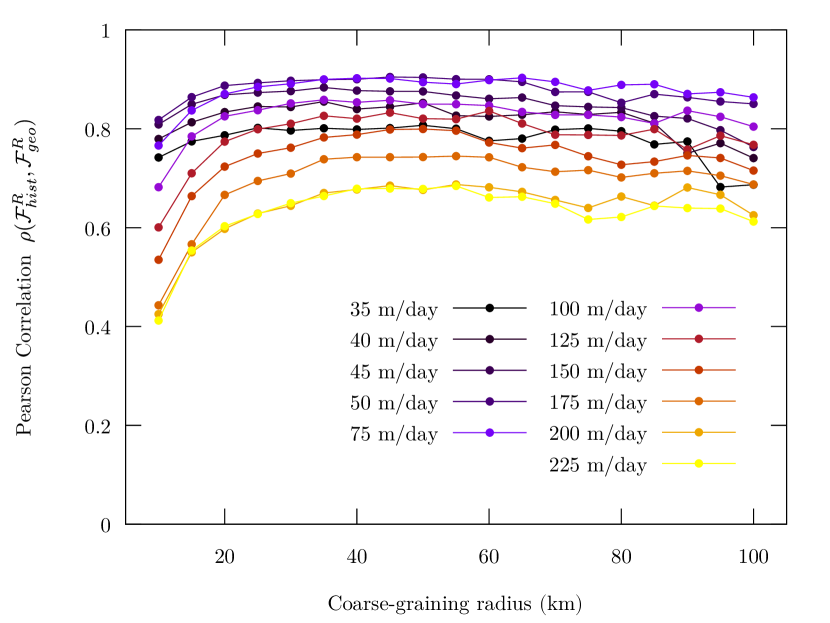
Figure 4: Pearson correlation coefficient between $\mathcal{F}^{R}_{\mathrm{geo}}$ and $\mathcal{F}^{R}_{\mathrm{hist}}$ as a function of the coarse-graining radius $R$. Color indicates different values of $v_{\mathrm{s}}$.

Maps of the density factor reveal the inhomogeneities of spatial patterns of sedimented particles produced by oceanic flows. The direct computation is shown in Figures 3a and 3c for two different settling velocities. Considerable inhomogeneities are evident: variations of the original density up to factors of $0.5$ and $1.5$ are common in Figure 3a. In general, inhomogeneities are stronger in the southern part of the domain, corresponding to the region of highest mesoscale activity (Hernández-Carrasco ., 2014). Also, inhomogeneities are stronger for smaller settling velocity (note the different color scales in the respective panels of Figure 3).

In Figures 3b and 3d we show the density factor obtained from the corresponding geometrical computation, properly coarse-grained (see section 2.5). A visual comparison with Figures 3a and 3c reveals almost identical patterns. Slightly more differences are noticeable for the larger value of the settling velocity. At high $v_{\mathrm{s}}$ and small $R$ (not shown) we have noticed that the direct sampling estimation is more noisy than the geometrical approach.

The quantitative comparison between the coarse-grained geometrical estimation of the density factor and the direct sampling one, shown in Figure 4, gives positive values for $\rho(\mathcal{F}^{R}_{\mathrm{hist}},\mathcal{F}^{R}_{\mathrm{geo}})$, ranging from $0.5$ to $0.9$ for all settling velocities and coarse-graining radii tested. For the majority of these parameter values, the correlation coefficient is above $0.7$, which indicates a relative insensitivity to flow scales below the mesoscale, which we model here by the presence of the noise term in the calculation of $\mathcal{F}^{R}_{\mathrm{hist}}$. Figure 4 also illustrates that the correlation is lower for the largest and smaller values of $R$. However, we find a wide range, from $R\approx 25$ to $75\mathrm{km}$, where high correlations between the two calculations occur for any settling velocity.

We study in Figure 5a the dependence of $\rho(\mathcal{F}^{R}_{\mathrm{hist}},\mathcal{F}^{R}_{\mathrm{geo}})$ on the settling velocity (purple symbols). We find it to be affected by $v_{\mathrm{s}}$ more than by $R$. That is, the nature (size and density, equation (1)) of the biogenic particles is what determines the difference between the two calculation methods, one restricted to mesoscales and another adding an extra term, which cannot be eliminated by an appropriate choice for the coarse-graining radius. $\rho(\mathcal{F}^{R}_{\mathrm{hist}},\mathcal{F}^{R}_{\mathrm{geo}})$ achieves its maximum for $v_{\mathrm{s}}=75\mathrm{m/day}$, roughly independently of $R$, and decreases fast and slowly for smaller and larger values of $v_{\mathrm{s}}$, respectively.

We next turn to analyzing the mechanisms from which the inhomogeneities originate. We do so by comparing the coarse-grained density factors $\mathcal{F}^{R}_{\mathrm{hist}}$ and $\mathcal{F}^{R}_{\mathrm{geo}}$ with the coarse-grained stretching ($\mathcal{S}^{R}$) and projection ($\mathcal{P}^{R}$) factors. Already Figure 5a makes clear that the stretching factor is correlated increasingly well with the density factor for increasing $v_{\mathrm{s}}$. According to Figure 5b, $\rho(\mathcal{F}^{R}_{\mathrm{geo}},\mathcal{S}^{R})$ approaches almost $1$ for high values of $v_{\mathrm{s}}$, i.e., stretching determines inhomogeneities almost alone for fast-sinking particles. The opposite occurs when lowering $v_{\mathrm{s}}$, but the trend reverses again for very low values of the settling velocity. The dependence on $v_{\mathrm{s}}$ is quite robust against changing $R$.

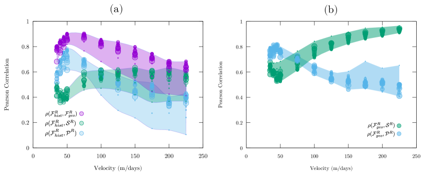
Figure 5: a) Pearson correlation between $\mathcal{F}^{R}_{\mathrm{geo}}$ and $\mathcal{F}^{R}_{\mathrm{hist}}$ (magenta circles), $\mathcal{F}^{R}_{\mathrm{hist}}$ and $\mathcal{S}^{R}$ (green circles) and $\mathcal{F}^{R}_{\mathrm{hist}}$ and $\mathcal{P}^{R}$ (blue circles) as a function of the settling velocity $v_{\mathrm{s}}$. b) Pearson correlation between $\mathcal{F}^{R}_{\mathrm{geo}}$ and $\mathcal{S}^{R}$ (green circles) and $\mathcal{F}^{R}_{\mathrm{geo}}$ and $\mathcal{P}^{R}$ (blue circles) as a function of the settling velocity. Circle size corresponds to the coarse-graining or sampling radius $R$. Shaded areas indicate the full range of values.

Figure 6 characterizes the degree of inhomogeneity in terms of the spatial standard deviation of the coarse-grained density factor, as well as the quantities characterizing the two mechanisms involved, the stretching and projection coarse-grained factors, as a function of $t_{\mathrm{f}}=\frac{|z-z_{0}|}{v_{\mathrm{s}}}$. This quantity is proportional to the inverse of the settling velocity, and approximately corresponds to the mean arrival time of the particles to the accumulation depth. Using $t_{\mathrm{f}}$ allows a more intuitive interpretation of the results. In the investigated domain, the degree of inhomogeneity in all factors grows with the time available for sinking, as shown in Figure 6. We find that the growth of the standard deviations of $\mathcal{S}^{R}$ and $\mathcal{P}^{R}$ with $t_{\mathrm{f}}$ is well described by power laws, $t_{\mathrm{f}}^{\alpha}$, with approximate exponents $\alpha\approx 1$ and $5/3$, respectively. Not surprisingly in view of figure 5, which indicates a dominance of stretching and of projection at large and at small values of $v_{\mathrm{s}}\propto t_{\mathrm{f}}^{-1}$, respectively, $\mathcal{F}_{\mathrm{geo}}^{R}$ reflects the power-law of exponent $1$ for short values of $t_{\mathrm{f}}$ and crossovers to the exponent $5/3$ at larger $t_{\mathrm{f}}$. The standard deviation of $\mathcal{F}_{\mathrm{hist}}^{R}$ practically coincides with that of $\mathcal{F}_{\mathrm{geo}}^{R}$ (Figure 6d), which means that the dependence on $t_{\mathrm{f}}$ as appearing in the direct sampling method can be traced back to a combination of the mentioned power laws corresponding to the two basic geometrical mechanisms, and that only the mesoscales included in $\mathcal{F}_{\mathrm{geo}}^{R}$ turn out to be relevant.

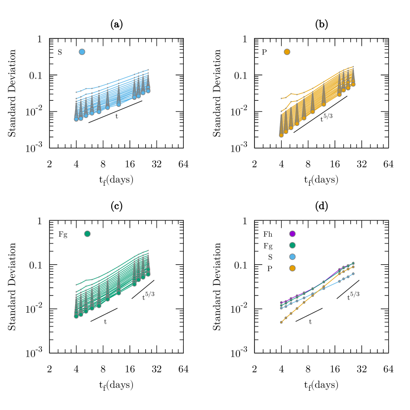
Figure 6: Spatial standard deviation of $\mathcal{S}^{R}$ (a), $\mathcal{P}^{R}$ (b) and $\mathcal{F}_{\mathrm{geo}}^{R}$ (c) as a function of $t_{\mathrm{f}}=|z-z_{0}|/v_{\mathrm{s}}$, which approximately corresponds to the mean arrival time. The size of the circles represents the coarse-graining radius $R$. Panel (d) displays the spatial standard deviations of $\mathcal{F}_{\mathrm{hist}}^{R}$, $\mathcal{F}_{\mathrm{geo}}^{R}$, $\mathcal{S}^{R}$ and $\mathcal{P}^{R}$ for one coarse-graining resolution, $R=50\mathrm{km}$.

So far, we have investigated results obtained by coarse-graining, which smoothes out any extreme inhomogeneities if they are present. Indeed we have used a rather large coarse-graining radius $R$, as appropriate for the statistical analysis performed above and to discuss large-scale features of the sedimented density. At the same time, the calculation of $\mathcal{F}_{\mathrm{geo}}$ does not involve coarse-graining, so that arbitrarily fine details can be visualized in principle. With velocity data of sufficiently high resolution, this geometrical approach would be more appropriate to discuss results from the relatively small collecting area of sediment traps. In Figure 7a we show the counterpart of Figure 3b (only for the gray rectangle) without coarse-graining. The main difference is the presence of extremely high values. They presumably correspond to projection factors being close to produce projection caustics, similar to those found in Drótos . (2019), which will be discussed in section 4.2. Both their spatial abundance and the corresponding numerical values of the density factor increase as the settling velocity decreases (not shown). We note that the degree of inhomogeneity, including the abundance of extreme values, is larger in the southern part of the area. This difference is presumably related to the stronger turbulence in the southern upwelling region as documented in Hernández-Carrasco . (2014). Stronger turbulence is associated to larger stretching and also more complex shapes (more tiltness) for the layer of sinking particles (Goto  Kida, 2007).

The degree of inhomogeneity may be better visualized by taking linear cross-sections of Figure 7a. Figure 7b shows cross-sections taken at constant latitudes. One can observe that inhomogeneities are moderate in the northern part but strong at some southern latitudes. At $16^{\circ}\mathrm{S}$, hardly a factor of 2 is reached between the smallest and the largest values, while the same increment is common even within less than $1^{\circ}$ separation at the other two latitudes shown in Fig. 7b. Near $10^{\circ}\mathrm{E}$ longitude, factor 5 increments appear in the $32^{\circ}\mathrm{S}$ cross-section on quite small scales, and a much larger factor, more than 10, in a situation close to caustic formation, is visible in the $24^{\circ}\mathrm{S}$ cross-section.

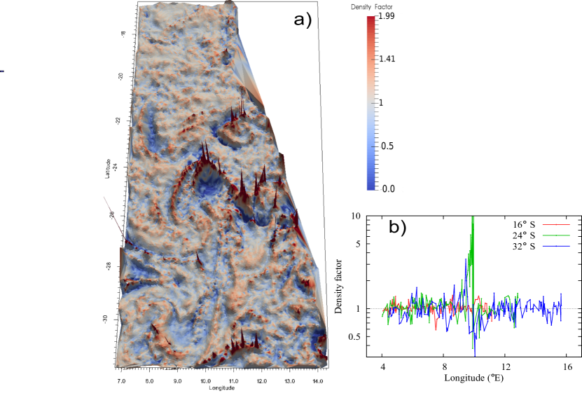
Figure 7: Results for the density factor $\mathcal{F}_{\mathrm{geo}}$ numerically estimated by the geometrical expression (4) for the particle locations within the accumulation level, for a settling velocity of $50\mathrm{m}/\mathrm{day}$. Further parameters are as in Table 1. (a) The surface was interpolated applying Delaunay triangulation to the values of the density factor at the particles’ ending positions. The color and the height of the surface corresponds to the value of the density factor. Note that there are some localized extreme values that are well outside the range covered by the color bar. (b) Zonal cross-sections taken at the indicated latitudes. These cross-sections were built by selecting those trajectories whose endpoints are closer than $1/48$ degrees to the given latitude. This choice was found to ensure the comparability of zonal and meridional distances between neighboring trajectories.

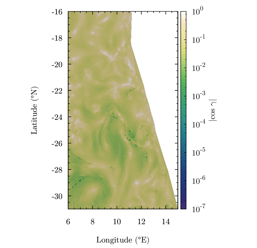
Figure 8: Results for the local value of $|\cos\gamma|$ for the same simulation and using the same Delaunay representation as in Figure 7.

4 Discussion

4.1 The relative importance of stretching and projection in the density factor

We found that the correlations of $\mathcal{S}^{R}$ and $\mathcal{P}^{R}$ with $\mathcal{F}^{R}_{\mathrm{geo}}$ behave differently as a function of $v_{\mathrm{s}}$ (see Figure 5): For increasing settling velocities or decreasing $t_{\mathrm{f}}$, $\rho(\mathcal{F}^{R}_{\mathrm{geo}},\mathcal{S}^{R})$ becomes higher and approaches $1$, whereas $\rho(\mathcal{F}^{R}_{\mathrm{geo}},\mathcal{P}^{R})$ decreases, implying that the stretching mechanism becomes dominant for fast sinking (and thus short settling time). For very low values of $v_{\mathrm{s}}$, however, the trends reverse.

Note that the Pearson correlation coefficient carries information about co-occurrence of fluctuations around averages. In our case, if the non-coarse-grained $\mathcal{S}$ and $\mathcal{P}$ were uncorrelated, one would find $\rho(\mathcal{F}_{\mathrm{geo}},\mathcal{S})=\frac{\sigma_{\mathcal{S}}}{\sigma_{\mathcal{F}_{\mathrm{geo}}}}\langle\mathcal{P}\rangle$, where $\langle\mathcal{P}\rangle$ is the spatial mean of $\mathcal{P}$, and a similar formula for $\rho(\mathcal{F}_{\mathrm{geo}},\mathcal{P})$. Although the spatial fluctuations of $\mathcal{S}$ and $\mathcal{P}$ are actually not independent, the spatial means of $\mathcal{S}$ and $\mathcal{P}$ are not investigated, and Figure 5 presents coarse-grained quantities, the relationships between the Pearson correlation coefficients and the standard deviations might have some explanatory power in view of Figure 6: the linear and the $5/3$-power scaling of the standard deviation of $\mathcal{S}$ and $\mathcal{P}$ with $t_{\mathrm{f}}\propto v_{\mathrm{s}}^{-1}$ might make them dominate for small and large $t_{\mathrm{f}}$, respectively.

One should also note that short integration times, corresponding to high settling velocities, make the layer of particles arrive at the accumulation level approximately horizontally, i.e., tiltness does not have time to develop. Therefore, the normal vector $\mathbf{n}$ of the layer is pointing nearly vertically upwards, $\beta\approx\gamma$ and, from equation (6), $\mathcal{P}\approx 1$. Consequently, the (non-coarse-grained) density factor will satisfy $\mathcal{F}_{\mathrm{geo}}\approx\mathcal{S}$. Additionally, in this or in any other situation in which the sinking layer remains nearly horizontal during all the settling process, the stretching factor can be approximated (see equation (23)) as

$$\mathcal{S}=\exp{\left(-\int_{t_{0}}^{t_{z}}\nabla_{\mathrm{h}}\cdot\mathbf{v}dt^{\prime}\right)},$$ (13)

where $\nabla_{\mathrm{h}}\cdot\mathbf{v}=\partial_{x}v_{x}+\partial_{y}v_{y}$ is the horizontal divergence of the velocity field. This exponential expression for the density factor was proposed heuristically in Monroy . (2017) and found to be a reasonable approximation. Note that $\exp{\left(-\int_{t_{0}}^{t_{z}}\nabla_{\mathrm{h}}\cdot\mathbf{v}dt^{\prime}\right)}$ can be transformed to $\exp{\left(\int_{t_{0}}^{t_{z}}\partial_{z}v_{z}dt^{\prime}\right)}$ by taking into account incompressibility. This means that the stretching factor (and thus the complete density factor) can be obtained from the temporal average of the vertical shear felt by the sinking particles when the sinking sheet remains almost horizontal, e.g. for high settling velocities. Although $\mathcal{S}\approx 1$ as well in this case, our numerical experience indicates that $\mathcal{S}$ tends to $1$ slower than $\mathcal{P}$ for increasing settling velocity, and the evaluation of the discussed exponential expression thus becomes sound.

For small settling velocities, the trends of the curves in Figure 5 reverse: the importance of stretching increases again with respect to projection. This may be a consequence of the phenomenon observed by Drótos . (2019) in a simplified kinematic flow: effects due to tiltness (which determines $\mathcal{P}$) saturate for long settling times, whereas effects due to stretching can grow to arbitrarily large values. The power-law behavior of the standard deviation of $\mathcal{P}$ identified in Fig. 6b could contradict this explanation, but the lines in this figure actually deviate downward from the power law for long settling times.

4.2 About the presence of extreme inhomogeneities and caustics

We found extremely large values of the geometric density factor, and thus of the accumulated density, in particular locations on the collecting surface (see Figure 7). We associate them to configurations close to projection caustics (Drótos ., 2019). These are locations where the direction of the velocity $\mathbf{v}$ and the direction normal to the layer of particles, $\mathbf{n}$, become perpendicular so that

$$\cos\gamma\equiv\mathbf{n}\cdot\frac{\mathbf{v}}{v}=0\ ,$$ (14)

and then the projection factor $\mathcal{P}_{\mathrm{geo}}$ (equation (6)) becomes infinite. Geometrically, the condition in equation (14) occurs when the sinking layer appears folded when projected on the collecting surface along the direction of motion.

Numerical values for $\cos\gamma=\mathbf{n}\cdot\mathbf{v}/v$ are shown in Figure 8 for the same simulation as in Figure 7. It becomes obvious that most of the high values of the density factor in Figure 7 arise where $\cos\gamma$ takes small values, i.e. a situation close to produce a projection caustic. In generic three-dimensional flows in which the sinking surface folds while sinking, caustics will occur as one-dimensional curves on the collecting surface, across which the sign of $\cos\gamma$ would change. Figure 8, however, shows small but non-vanishing values of $\cos\gamma$, and sign reversal does not occur. In contrast with generic three-dimensional flows, mesoscale oceanic flows have special properties. As mentioned, even an initially horizontal particle layer would become tilted, but gradients in the vertical velocity component are small in the ocean (LaCasce  Bower, 2000), so the tiltness (the direction of the normal vector $\mathbf{n}$) cannot change very much. Therefore, the particles must have nearly horizontal local velocity $\mathbf{v}$ in order to have it perpendicular to $\mathbf{n}$ and caustics to appear. Actually, the vertical component of the velocity field of the fluid is orders of magnitude smaller than horizontal components in the ocean, even in the Benguela region, which contains upwelling cells (Rossi ., 2008) with enhanced vertical flows. Although the addition of the settling velocity $\mathbf{v}_{\mathrm{s}}$ increases the magnitude of the vertical component of the particle velocity $\mathbf{v}$, it still remains much smaller than the horizontal components. Consequently, $\mathbf{v}$ is close to horizontal, i.e., the approach angle to the accumulation depth is low (Siegel  Deuser, 1997; Buesseler ., 2007), so that caustics might finally appear. However, the settling velocity $v_{\mathrm{s}}=50$ m/day used in Figures 7 and 8 is too large, and the perpendicularity property required by equation (14) is not really achieved, although it is closely approached in particular locations of the collecting surface. We expect that locations with even higher densities and even true projection caustics would appear if using smaller values of $v_{\mathrm{s}}$. Additionally, one may suspect that a longer sinking time gives more opportunity to form foldings and to larger deviation of $\mathbf{n}$ from vertical. The practical implication of these considerations, as far as the effect of the projection factor $\mathcal{P}$ is concerned, is that very small or light (thus slow) particles will present a more irregular settling distribution than the ones sinking faster. This is indeed the trend observed in Figures 3 and 6.

We note that, as shown in Drótos . (2019), the extremely high values involved in caustics are smoothed out if a full three-dimensional volume of particles is considered to sink instead of a thin layer. Also, any coarse-graining is expected to efficiently filter out extremely high density values, even for a small coarse-graining radius $R$, as our results in section 3 suggest. We can conclude that true projection caustics will not be readily observed in distributions of settling particles in ocean flows, but they will leave a trace of highly inhomogeneous distributions for the lighter and smaller types of particles.

4.3 Other aspects

Figure 5a shows that the agreement between $\mathcal{F}^{R}_{\mathrm{hist}}$ and $\mathcal{F}^{R}_{\mathrm{geo}}$ deteriorates with increasing values of the settling velocity $v_{\mathrm{s}}$ (and also at very small values of it). Besides the technical differences arising from their definitions, the main physical difference between them is that $\mathcal{F}^{R}_{\mathrm{geo}}$ has been computed using exclusively a mesoscale flow, whereas an additional noise term has been included in the calculation of $\mathcal{F}^{R}_{\mathrm{hist}}$. This term is a crude way to introduce flow scales below mesoscales. In any case, a good agreement between $\mathcal{F}^{R}_{\mathrm{hist}}$ and $\mathcal{F}^{R}_{\mathrm{geo}}$ in Figures 4 and 5a should be interpreted as a confirmation of the insensitivity of the density factor to particular types of flow perturbations below mesoscale. In particular, from Figure 5a we see that the best agreement occurs for values of $t_{\mathrm{s}}$ for which the dominant source of inhomogeneity is the projection factor.

In general, we find larger density inhomogeneities (Figures (3) and (7)) in the southern part of the Benguela region. This is presumably related to the much stronger presence of mesoscale structures there, as discussed for the upper ocean layers in Hernández-Carrasco . (2014). This would indicate that mesoscale turbulence enhances the inhomogeneities in the settling process, which would not be surprising since stronger turbulence introduces more spatial variability in all relevant processes (Goto  Kida, 2007).

We emphasize that the analytical expressions for the density factor hold separately for each trajectory. Our assumption of a homogeneous initial density is useful for the characterization of the pure effect of transport. But in the case of an inhomogeneous particle release, the full density at the bottom can be readily obtained at the final location of each trajectory within our framework if the initially released density is known (for example by estimating it from primary production data). This is simply done by the multiplication of the initial density with the density factor associated to the corresponding trajectory.

In a realistic setting, unlike in our analyses, particles with different physical characteristics are present. Since the spatial pattern of the geometric density factor depends very strongly on the settling velocity, the effect of transport can cause separation of different types of particles, in a similar way to the effect of inertia at smaller scales considered in Font-Muñoz . (2017).

We have used a particular ROMS velocity field which properly resolves mesoscales. Improving the model resolution will give access to still more realistic velocities from which more realistic sedimentation patterns can be obtained. Our result that the inhomogeneities are determined by the stretching and projection mechanisms is not affected by that. Furthermore, the quantitative comparisons of density factors, with and without noise added to the velocities (Figures 3-5), indicate that large-scale features of the sedimented density are rather robust to small-scale details in the velocity field, like the ones that appear if increasing model resolution (while the small scales of the sedimentation pattern, relevant for data from an individual sediment trap, would be altered). This is further confirmed by some computations performed with the same ROMS velocity field undersampled to a lower horizontal resolution ($1/6^{\circ}$) with a proportionally larger value of the coarse-graining radius $R$. We note, however, that care should be taken to check numerical convergence and avoid artifacts when changing velocity-field resolution, since the resolution of the grid of particle deployment in the upper layer, the velocity interpolation methods, or the values of the coarse-graining radius may need to be adapted.

5 Conclusions

We have shown that common types of particles of biogenic origin, when sedimenting towards the deep ocean, do so in a inhomogeneous manner, which we have characterized with the horizontal dependence of the accumulated density at a given depth. These inhomogeneities are present even if particles are produced in a completely homogeneous manner in the upper ocean layers, and they arise from the effects of the flow while the particles are sinking.

For the case of particles homogeneously initialized in a horizontal sheet close to the ocean surface, we have adapted analytical expressions derived earlier (Drótos ., 2019) that allow identifying the mechanisms leading to the inhomogeneities: stretching of the sinking sheet, and its projection on a deep horizontal surface when the particles reach that depth. For large settling velocities, the stretching mechanism becomes dominant, and projection gains relevance for smaller settling velocities or, equivalently, for longer settling times. The degree of inhomogeneity grows as the settling time increases. We observe numerically that this growth follows specific power laws for each of the two mechanisms involved. Further work could try to find analytical explanations for them.

In a range of settling velocities, our results are robust to the introduction of flow perturbations by noise which try to model small-scale processes not included in the mesoscale flow. Within a reasonable range, results are also robust to the size of the coarse-graining scale introduced to make consistent comparisons.

The settling velocity has been one of the main parameters, but we stress that changing it is equivalent to considering different physical properties of the sinking particles, so that we are indeed scanning a variety of particle types. Particles sinking faster display weaker inhomogeneities in the accumulated density as compared to ones sinking more slowly.

Although our study has been limited to particles homogeneously initialized in a horizontal sheet, more general release configurations can be understood in terms of this simplified setup (Drótos ., 2019). A further limitation is posed by the biogeochemical and (dis)aggregation processes occurring during the sedimentation process, which are neglected in our framework and would need to be considered in future studies.

Appendices

Appendix A Density factor, geometrical approach

Here we derive equation (5) for the stretching factor $\mathcal{S}\equiv dA_{0}/dA_{t_{z}}$, where $dA_{0}$ is an infinitesimal area element on the horizontal surface where the particle with trajectory $\mathbf{R}=\mathbf{R}(\mathbf{r}_{0},t)$ was initialized at $t=t_{0}$, and $dA_{t_{z}}$ is the area of that element after evolution until time $t_{z}$, when the particle reaches depth $z$. We denote the zonal, meridional and vertical components of the vectors involved as $\mathbf{R}=(X,Y,Z)$ and $\mathbf{r}_{0}=(x_{0},y_{0},z_{0})$.

Let $d_{x}\mathbf{R}(\mathbf{r_{0}},t)$ be a vector giving the separation at all time of two particles that where initially separated by an infinitesimal distance $dx_{0}$ along the zonal direction on the initialization surface:

$$d_{x}\mathbf{R}(\mathbf{r_{0}},t)\equiv\mathbf{R}(x_{0}+dx_{0},y_{0},z_{0},t)-\mathbf{R}(x_{0},y_{0},z_{0},t)=\frac{\partial\mathbf{R}(\mathbf{r_{0}},t)}{\partial x_{0}}dx_{0}\equiv\mathbf{\tau}_{x}(t)dx_{0},$$ (15)

where we have introduced the vector $\mathbf{\tau}_{x}(t)$ as in equation (7). It is a vector tangent to the sinking surface at any time. Since $\mathbf{R}(\mathbf{r}_{0},t_{0})=\mathbf{r}_{0}$, $\mathbf{\tau}_{x}(t_{0})$ is a unit vector pointing in the zonal direction. Analogously we have

$$d_{y}\mathbf{R}(\mathbf{r_{0}},t)\equiv\mathbf{R}(x_{0},y_{0}+dy_{0},z_{0},t)-\mathbf{R}(x_{0},y_{0},z_{0},t)=\frac{\partial\mathbf{R}(\mathbf{r_{0}},t)}{\partial y_{0}}dy_{0}\equiv\mathbf{\tau}_{y}(t)dy_{0}.$$ (16)

Let us choose as initial patch of area $dA_{0}$ in equation (4) the square spanned by the vectors $d_{x}\mathbf{R}(\mathbf{r}_{0},t_{0})$ and $d_{y}\mathbf{R}(\mathbf{}r_{0},t_{0})$, i.e., $dA_{0}=dx_{0}dy_{0}$. Since $d_{x}\mathbf{R}$ and $d_{y}\mathbf{R}$ are tangent to the sinking patch at any time, their cross product $d_{x}\mathbf{R}\times d_{y}\mathbf{R}$ gives at any time a vector normal to this patch (i.e. in the direction of the unit normal vector $\mathbf{n}$), with modulus $dA_{t}$ giving the area of the patch. Thus

$$\mathbf{n}dA_{t}=d_{x}\mathbf{R}\times d_{y}\mathbf{R}=(\mathbf{\tau}_{x}(t)\times\mathbf{\tau}_{y}(t))dx_{0}dy_{0}=(\mathbf{\tau}_{x}(t)\times\mathbf{\tau}_{y}(t))dA_{0}.$$ (17)

Particularizing to the time $t_{z}$ at which the trajectory $\mathbf{R}(\mathbf{r}_{0},t)$ reaches the accumulation surface at depth $z$, we find $\mathcal{S}=dA_{0}/dA_{t_{z}}=|\mathbf{\tau}_{x}(t_{z})\times\mathbf{\tau}_{y}(t_{z})|^{-1}$, as in equation (5).

An interesting expression can be obtained in the particular situation in which the sinking surface remains horizontal at all times. In this case, the vector $\mathbf{\tau}_{x}(t)\times\mathbf{\tau}_{y}(t)$ has only vertical, $z$, component, which can be written in terms of a horizontal Jacobian determinant $|J_{\mathrm{h}}|$:

$$\mathcal{S}^{-1}=\left(\mathbf{\tau}_{x}(t)\times\mathbf{\tau}_{y}(t)\right)_{z}=|J_{\mathrm{h}}|\equiv\left|\frac{\partial(X,Y)}{\partial(x_{0},y_{0})}\right|=\begin{vmatrix}\frac{\partial X}{\partial x_{0}}&\frac{\partial X}{\partial y_{0}}\\ \frac{\partial Y}{\partial x_{0}}&\frac{\partial Y}{\partial y_{0}}\end{vmatrix}.$$ (18)

On the other hand, a standard equation for the time evolution of the three-dimensional Jacobian matrix $J_{ij}=\partial R_{i}/\partial x_{0j}$, $i,j=x,y,z$ can be obtained:

$$\frac{d}{dt}J_{ij}=\frac{d}{dt}\frac{\partial R_{i}}{\partial x_{0j}}=\frac{\partial v_{i}}{\partial x_{0j}}=\sum_{k=x,y,z}\frac{\partial v_{i}}{\partial R_{k}}\frac{\partial R_{k}}{\partial x_{0j}}=\sum_{k=x,y}\frac{\partial v_{i}}{\partial R_{k}}\frac{\partial R_{k}}{\partial x_{0j}}+\frac{\partial v_{i}}{\partial Z}\frac{\partial Z}{\partial x_{0j}},\quad i,j=x,y,z.$$ (19)

In the last equality we have separated the contribution from the vertical coordinate, and all derivatives there are taken at constant $t$. We recognize that the matrix $J_{\mathrm{h}}$ whose determinant appears in equation (18) has the components of $J_{ij}$ with $i,j=x,y$. Thus:

$$\frac{d}{dt}(J_{\mathrm{h}})_{ij}=\sum_{k=x,y}\frac{\partial v_{i}}{\partial R_{k}}\frac{\partial R_{k}}{\partial x_{0j}}+\frac{\partial v_{i}}{\partial Z}\frac{\partial Z}{\partial x_{0j}},\quad i,j=x,y.$$ (20)

Under the assumption that the sinking surface remains horizontal at all times, we have $\partial Z/\partial x_{0j}=0$ for $j=x,y$, and then equation (20) can be written in matrix form as

$$\frac{d}{dt}J_{\mathrm{h}}=(\nabla_{\mathrm{h}}\mathbf{v}_{\mathrm{h}})^{T}J_{\mathrm{h}}\ .$$ (21)

$\nabla_{\mathrm{h}}\mathbf{v}_{\mathrm{h}}$ is the horizontal velocity gradient matrix containing the derivatives of the horizontal components of the velocity with respect to the horizontal coordinates. The superindex $T$ indicates transpose.

From equation (21):

$$\frac{1}{|J_{\mathrm{h}}|}\frac{d|J_{\mathrm{h}}|}{dt}=Tr\left(\frac{dJ_{\mathrm{h}}}{dt}J_{\mathrm{h}}^{-1}\right)=Tr\left(\nabla_{\mathrm{h}}\mathbf{v}_{\mathrm{h}}\right)=\nabla_{\mathrm{h}}\cdot\mathbf{v}_{\mathrm{h}},$$ (22)

where we have used the Jacobi formula in the first equality ($Tr(M)$ means trace of the matrix $M$). $\nabla_{\mathrm{h}}\cdot\mathbf{v}_{\mathrm{h}}=\partial_{x}v_{x}+\partial_{y}v_{y}$ is the horizontal divergence of the particle velocity field, which is, since the settling velocity is constant, also the horizontal divergence of the fluid velocity field. Finally, combining (18) and (22), we obtain

$$\mathcal{S}=e^{-\int_{t_{0}}^{t}\nabla_{\mathrm{h}}\cdot\mathbf{v}_{\mathrm{h}}dt^{\prime}}.$$ (23)

Because of fluid incompressibility $\nabla_{\mathrm{h}}\cdot\mathbf{v}_{\mathrm{h}}=-\partial_{z}v_{z}$, one can also write

$$\mathcal{S}=e^{\int_{t_{0}}^{t}\partial_{z}v_{z}dt^{\prime}}.$$ (24)

Equations (23)-(24) give also the total density factor, $\mathcal{F}=\mathcal{S}$, since for a horizontal surface the projection factor $\mathcal{P}$ is unity. They express stretching and the density factor for a horizontally sinking surface in terms of the horizontal divergence and the vertical shear of the velocity field. Equation (23) was heuristically proposed in Monroy . (2017) and found to give a reasonable qualitative description of the density factor in the Benguela region. As a special case, (23) can also be obtained by assuming the projection factor tending to $1$ faster than (23) itself when a parameter is changing (like $\mathbf{v}_{\mathrm{s}}$ as discussed in section 4.1). A more precise description, however, needs the use of the complete factor $\mathcal{F}=\mathcal{S}\mathcal{P}$ with stretching and projection given by equations (5) and (6).

As a generalization of equation (23), valid for arbitrary orientation of the sinking surface, an expression alternative to equation (5) can be obtained manipulating equation (20). First we recognize that, for arbitrary orientation of the sinking patch, $|J_{\mathrm{h}}|$ gives the $z$ component of the vector $\mathbf{\tau}_{x}(t)\times\mathbf{\tau}_{y}(t)$. Using equation (5) and the vertical component of equation (8) we have

$$n_{z}=|J_{\mathrm{h}}|\mathcal{S}.$$ (25)

Now, using the full form of equation (20), equation (22) is replaced by

$$\frac{1}{|J_{\mathrm{h}}|}\frac{d|J_{\mathrm{h}}|}{dt}=Tr\left(\frac{dJ_{\mathrm{h}}}{dt}J_{\mathrm{h}}^{-1}\right)=\nabla_{\mathrm{h}}\cdot\mathbf{v}_{\mathrm{h}}+\nabla_{\mathrm{h}}Z\cdot\partial_{z}\mathbf{v}_{\mathrm{h}},$$ (26)

where $z=Z(x,y;t)$ gives the time-dependent depth of the sinking surface in terms of the horizontal coordinates. In the last term we have used the chain rule involving $(J_{\mathrm{h}}^{-1})_{ij}=\partial x_{0i}/\partial R_{j}$ for $i,j=x,y$. This expression is true if $x_{0i}$ is expressed as a function of $X$ and $Y$, with $z_{0}$ a parameter which is kept constant. From equations (25) and (26) we get

$$\mathcal{S}=n_{z}e^{-\int_{t_{0}}^{t}\left(\nabla_{\mathrm{h}}\cdot\mathbf{v}_{\mathrm{h}}+\nabla_{\mathrm{h}}Z\cdot\partial_{z}\mathbf{v}_{\mathrm{h}}\right)dt^{\prime}}.$$ (27)

We note that the integrand in the exponent of this last expression is $\partial_{x}v_{x}(x,y,Z(x,y;t);t)+\partial_{y}v_{y}(x,y,Z(x,y;t);t)$. Equation (27) reduces to (23) for a horizontal surface ($\nabla_{\mathrm{h}}Z=0$ and $n_{z}=1$).

Appendix B Numerical computation of the geometrical density factor

In the setup of our numerical experiment, the density inhomogeneities arise during the sedimentation of a particle layer initialized horizontally at a depth of $100\mathrm{m}$. The numerical evaluation of the density factor is applied separately for every particle trajectory tracked, so that it is obtained at each horizontal location $\mathbf{x}$ where a tracked particle reaches the collecting surface.

The tracked particle, which started at position $\mathbf{r}_{0}$ in the initial layer at time $t_{0}$, has trajectory $\mathbf{R}(\mathbf{r}_{0},t)$. In order to numerically compute the density factor $\mathcal{F}(\mathbf{x})$ at its ending location at a depth of $1000\mathrm{m}$, we initialize four auxiliary particle trajectories, with initial positions modified in the zonal and meridional directions. These auxiliary trajectories are given by $\mathbf{R}(\mathbf{r}_{0}\pm\mathbf{\delta}_{x},t)$ and $\mathbf{R}(\mathbf{r}_{0}\pm\mathbf{\delta}_{y},t)$. The initial zonal and meridional distances $|\mathbf{\delta}_{x}|$ and $|\mathbf{\delta}_{y}|$ are chosen to be $\delta=10~{}\mathrm{km}$ in the numerical experiments. (Zonal and meridional distances are expressed in terms of longitude $\phi$ and latitude $\theta$ in radians by $x=\mathcal{R}\phi\cos\theta$ and $y=\mathcal{R}\theta$, where $\mathcal{R}$ is the radius of the Earth.) With the help of these auxiliary particle trajectories we compute the two tangent vectors of the particle layer using finite differences

$$\mathbf{\tau}_{x} \simeq \frac{\mathbf{R}(\mathbf{r}_{0}+\mathbf{\delta}_{x},t)-\mathbf{R}(\mathbf{r}_{0}-\mathbf{\delta}_{x},t)}{2\delta},$$

$$\mathbf{\tau}_{y} \simeq \frac{\mathbf{R}(\mathbf{r}_{0}+\mathbf{\delta}_{y},t)-\mathbf{R}(\mathbf{r}_{0}-\mathbf{\delta}_{y},t)}{2\delta}.$$ (28)

These tangent vectors $\mathbf{\tau}_{x}$, $\mathbf{\tau}_{y}$ and the velocity $\mathbf{v}$ of the reference trajectory at its ending position are used to compute the stretching factor $\mathcal{S}$ from equation (5) and the projection factor $\mathcal{P}$ from equation (6).

However, long integration times $t$ result in inaccurate estimations of the tangent vectors $\mathbf{\tau}_{x}$ and $\mathbf{\tau}_{y}$, because auxiliary particle trajectories move away excessively from the reference trajectory and leave the region where the estimation in equations (28) remains valid. We solve this issue by resetting the distance, with respect to the reference trajectory, and the orientation of the auxiliary trajectories to their initial configuration after each time interval of $\Delta t=1.5~{}\mathrm{days}$ using

$$\mathbf{R}(\mathbf{r}_{0}\pm\mathbf{\delta}_{x},t) \rightarrow \mathbf{R}(\mathbf{r}_{0},t)\pm\delta\frac{\mathbf{\tau}_{x}}{|\mathbf{\tau}_{x}|},$$

$$\mathbf{R}(\mathbf{r}_{0}\pm\mathbf{\delta}_{y},t) \rightarrow \mathbf{R}(\mathbf{r}_{0},t)\pm\delta\frac{\mathbf{\tau}_{x}}{|\mathbf{\tau}_{x}|}\times\mathbf{n}.$$

This renormalization procedure requires to store the value of the stretching factor $\mathcal{S}$ after every time interval $\Delta t$, with

$$\mathcal{S}(t_{0}+k\Delta t)=|\mathbf{\tau}_{x}(t_{0}+k\Delta t)\times\mathbf{\tau}_{y}(t_{0}+k\Delta t)|^{-1}.$$ (29)

The total stretching factor at the ending position (after $n$ time steps) is obtained as the product of the intermediate values:

$$\mathcal{S}=\prod_{k=1}^{n}\mathcal{S}(t_{0}+k\Delta t).$$ (30)

Once the stretching factor $\mathcal{S}$ and the projection factor $\mathcal{P}$ are numerically computed, their product gives the estimation of $\mathcal{F}_{\mathrm{geo}}(\mathbf{x})$, the density factor at the arrival point on the collecting surface, based on geometrical considerations.

Appendix C Coarse-graining of the geometrical density factor

The geometrical computation of the density factor obtains the value of $\mathcal{F}_{\mathrm{geo}}(\mathbf{x}_{i})$ at the endpoint $\mathbf{x}_{i}$ of each of the particles tracked until the collecting surface. The direct sampling calculation, however, gives a value $\mathcal{F}^{R}_{\mathrm{hist}}(\mathbf{x})$ associated to circles of radius $R$ around the sampling locations $\mathbf{x}$. In order to compare the two quantities we have to make some averaging or coarse-graining of the values of $\mathcal{F}_{\mathrm{geo}}(\mathbf{x}_{i})$ falling inside each of the sampling circles. But a simple arithmetic mean will have a bias to high values, because more particles fall in regions with higher density.

The appropriate approach is as follows: The coarse-grained value of the geometric density factor, $\mathcal{F}_{\mathrm{geo}}^{R}$, should be given by the ratio between the value of the accumulated density $\sigma_{z}^{R}$ on the lower surface, measured in one of the sampling circles of radius $R$, and the initial density $\sigma_{0}$. In the lower surface we have $\sigma_{z}^{R}=n_{R}/A^{R}_{\mathrm{acc}}$, where $A^{R}_{\mathrm{acc}}=\pi R^{2}$ is the area of one of the sampling circles and $n_{R}$ is the number of particles landing there. If we track back in time the trajectories of all points in this final area we will get an initial area $A_{0}$ containing the same number of particles $n_{R}$ at the initial time. Thus,

$$\mathcal{F}_{\mathrm{geo}}^{R}\equiv\frac{\sigma_{z}^{R}}{\sigma_{0}}=\frac{A_{0}}{A_{\mathrm{acc}}^{R}}.$$ (31)

Section 2.4 contains expressions for the evaluation of the ratio of areas in equation (31) when they are infinitesimal patches. But in general $A_{0}$ and $A_{\mathrm{acc}}^{R}$ will be too large to apply such expressions. We can solve this issue by noticing that we initialize the particles in the upper layer in a regular grid in zonal and meridional distances, so that we can associate the same small area $a_{0}$ (for example that of the unit cell of the grid or of the Voronoi cell) to each of the particles in the initial surface. Then, we can approximate the initial area $A_{0}$ by summing up all the small areas $a_{0}$ corresponding to each of the $n_{R}$ particles that will reach the sampling circle in the lower surface:

$$A_{0}\simeq n_{R}a_{0}.$$ (32)

If we use many particles so that they are initially very closely spaced, $a_{0}$ will be very small, and we can use the expression valid for the ratio of infinitesimal patches:

$$a_{\mathrm{acc},i}\simeq\frac{1}{\mathcal{F}_{\mathrm{geo}}(\mathbf{x}_{i})}a_{0},$$ (33)

where $a_{\mathrm{acc},i}$ is the area of the footprint left around the final location $\mathbf{x}_{i}$ by the sedimentation of the small patch of initial area $a_{0}$. The final area $A_{\mathrm{acc}}^{R}$ will be now covered by the areas $a_{\mathrm{acc},i}$:

$$A_{\mathrm{acc}}^{R}\simeq\sum_{i}^{n_{R}}a_{\mathrm{acc},i}.$$ (34)

The combination of equations (31)-(34) gives

$$\mathcal{F}_{\mathrm{geo}}^{R}\simeq\frac{n_{R}}{\sum_{i=1}^{n_{R}}\frac{1}{\mathcal{F}_{\mathrm{geo}}(\mathbf{x}_{i})}}.$$ (35)

That is, the proper estimation of the density factor in a finite area corresponds to the harmonic mean of the geometrical density factors of the trajectories involved, equation (10). Note that exact equalities hold for infinitely many particles.