Matching Quasi Generalized Parton Distributions in the RI/MOM scheme

Abstract

Within the framework of large momentum effective theory (LaMET), generalized parton distributions (GPDs) can be extracted from lattice calculations of quasi-GPDs through a perturbative matching relation, up to power corrections that are suppressed by the hadron momentum. In this paper, we focus on isovector quark GPDs, including the unpolarized, longitudinally and transversely polarized cases, and present the one-loop matching that connects the quasi-GPDs renormalized in a regularization-independent momentum subtraction (RI/MOM) scheme to the GPDs in $\overline{\rm MS}$ scheme. We find that the matching coefficient is independent of the momentum transfer squared. As a consequence, the matching for the quasi-GPD with zero skewness is the same as that for the quasi-PDF. Our results provide a crucial input for the determination of quark GPDs from lattice QCD using LaMET.

I Introduction

Understanding the internal structure of nucleons has been an important goal of hadron physics. For many decades, our knowledge on the structure of nucleons has been mainly relying on experimental measurements of their form factors (FFs) and parton distribution functions (PDFs). The FFs describe the spatial distribution of charge and current within the nucleon and can be probed in elastic lepton-nucleon scattering, while the PDFs characterize the longitudinal momentum distribution of quarks and gluons in the nucleon and can be measured in deep-inelastic scattering processes.

The proposal of generalized parton distributions (GPDs) (for a review, see e.g. Ji (2004); Diehl (2003); Belitsky and Radyushkin (2005)) provides a novel opportunity to characterize the partonic structure of nucleons. As a generalization of the PDFs to off-forward kinematics, the GPDs contain a wealth of new information on nucleon structure. They naturally encompass the FFs, PDFs as well as the distribution amplitudes (DAs), and offer a description of the correlations between the transverse position and longitudinal momentum of quarks and gluons inside the nucleon, thereby giving access to quark and gluon orbital angular momentum contributions to the nucleon spin. Experimentally, the GPDs can be accessed through hard exclusive processes like deeply virtual Compton scattering or meson production. Much effort has been devoted to measuring such processes at completed and ongoing experiments (HERA Adloff et al. (2001); Chekanov et al. (2003); Aktas et al. (2005); Airapetian et al. (2001, 2011, 2012), COMPASS Gautheron et al. (2010), JLab Defurne et al. (2015); Jo et al. (2015); Seder et al. (2015); Dudek et al. (2012)), and will be continued at planned future facilities such as EIC Accardi et al. (2016); Aschenauer et al. (2014) and EicC Chen (2018). Given the complicated kinematic dependence of GPDs, extracting them from the accumulated experimental data is in general rather difficult, and one usually needs to resort to certain models that allow for an extrapolation to kinematic regions that are not accessible directly Bacchetta (2016).

On the other hand, lattice effort of studying GPDs has been mainly focused on the computation of their moments Hagler et al. (2003); Gockeler et al. (2004); Schroers et al. (2004); Gockeler et al. (2005); Hagler et al. (2008); Brommel et al. (2007); Alexandrou et al. (2011). The full distribution can be reconstructed in principle if all their moments are known. However, the number of moments that are calculable on lattice is very limited, owing to power divergent mixing between different moments operators and increasing stochastic noise for high moments operators.

In the past few years, a new theoretical framework has been developed to circumvent the above difficulties, which is now known as the large momentum effective theory (LaMET) Ji (2013, 2014). According to LaMET, the GPDs can be extracted from lattice QCD calculations of appropriately constructed static-operator matrix elements, which are named the quasi-GPDs. The quasi-GPDs are usually hadron-momentum dependent but time independent, and thus can be readily computed on the lattice. After being renormalized nonperturbatively in an appropriate scheme, the renormalized quasi-GPDs can then be matched onto the usual GPDs through a factorization formula accurate up to power corrections that are suppressed by the hadron momentum Ji et al. (2015a); Xiong and Zhang (2015).

Since LaMET was proposed, a lot of progress has been achieved both with respect to the theoretical understanding of the formalism Xiong et al. (2014); Ji and Zhang (2015); Ji et al. (2015a); Xiong and Zhang (2015); Li (2016); Chen et al. (2016); Ishikawa et al. (2016); Chen et al. (2017a); Monahan and Orginos (2017); Radyushkin (2017); Zhang et al. (2017); Carlson and Freid (2017); Ishikawa et al. (2017); Xiong et al. (2017); Constantinou and Panagopoulos (2017); Ji et al. (2018a); Green et al. (2018); Chen et al. (2018a); Alexandrou et al. (2017a); Green et al. (2018); Chen et al. (2017b); Lin et al. (2018a); Chen et al. (2017c); Rossi and Testa (2017); Ji et al. (2017); Hobbs (2018); Jia et al. (2017); Wang et al. (2018); Stewart and Zhao (2018); Monahan (2018); Wang and Zhao (2018); Izubuchi et al. (2018); Xu et al. (2018a); Briceño et al. (2018); Xu et al. (2018b); Jia et al. (2018); Spanoudes and Panagopoulos (2018); Rossi and Testa (2018); Liu et al. (2018a); Ji et al. (2018b); Bhattacharya et al. (2019); Radyushkin (2019); Zhang et al. (2018); Li et al. (2018); Braun et al. (2018) and the direct calculation of PDFs from lattice QCD Lin et al. (2015); Chen et al. (2016); Lin et al. (2018a); Alexandrou et al. (2015, 2017b, 2017a); Chen et al. (2018a); Zhang et al. (2017); Chen et al. (2017d); Alexandrou et al. (2018a); Chen et al. (2018b, c); Alexandrou et al. (2018b); Lin et al. (2018b); Fan et al. (2018); Liu et al. (2018b). The prospects of extracting transverse momentum dependent (TMD) PDFs from lattice with LaMET has been investigated in Refs. Ji et al. (2015b, 2018c); Ebert et al. (2019a); Constantinou et al. (2019); Ebert et al. (2019b). In particular, a multiplicative renormalization of both the quark Ji et al. (2018a); Ishikawa et al. (2017); Green et al. (2018) and gluon Zhang et al. (2018); Li et al. (2018) quasi-PDFs has been established in coordinate space. This allows for a nonperturbative renormalization in the regularization-independent momentum subtraction (RI/MOM) scheme Martinelli et al. (1995). For the isovector quark quasi-PDFs, this has been carried out in Refs. Chen et al. (2018a); Stewart and Zhao (2018); Chen et al. (2018b); Lin et al. (2018b) (see also Constantinou and Panagopoulos (2017); Alexandrou et al. (2017a, 2018a)). The relevant hard matching kernel in the same scheme has also been computed up to one loop Stewart and Zhao (2018); Liu et al. (2018a, b). Despite limited volumes and relatively coarse lattice spacings, the state-of-the-art nucleon isovector quark PDFs determined from lattice data at the physical point have shown a reasonable agreement Chen et al. (2018b); Lin et al. (2018b); Alexandrou et al. (2018a) with phenomenological results extracted from the experimental data Dulat et al. (2016); Ball et al. (2017); Harland-Lang et al. (2015); Nocera et al. (2014); Ethier et al. (2017). Of course, a careful study of theoretical uncertainties and lattice artifacts is still needed to fully establish the reliability of the results.

As for the GPDs, there have been studies on the perturbative matching of the isovector quark quasi-GPDs Ji et al. (2015a); Xiong and Zhang (2015), which are free from contributions of disconnected diagrams and mixing with gluon quasi-GPDs. Such studies were performed in a transverse momentum cutoff scheme and therefore not well-suited for the lattice implementation. In this paper, we reconsider the one-loop matching for isovector quark quasi-GPDs in the RI/MOM scheme. The results can be used to match the quasi-GPDs calculated in lattice QCD and renormalized in the RI/MOM scheme onto the GPDs in $\overline{\rm MS}$ scheme.

The rest of the paper is organized as follows: In Sec. II, we establish our definitions and conventions. In Sec. III, we present a rigorous derivation of the factorization formula for the isovector quark quasi-GPD based on operator product expansion (OPE). Section IV and V are devoted to the RI/MOM renormalization and matching procedure, respectively. We also explain how to obtain the matching coefficients of DAs from the one-loop results of GPDs in Sec. V. Our summary is given in Sec. VI.

II Definitions and conventions

The parent function for the quark GPDs, which we call parent-GPD for simplicity, is defined from the Fourier transform of the off-forward matrix element of a light-cone correlator,

$$F(\bar{\Gamma},x,\xi,t,\mu)$$

$$=\int\frac{d\zeta^{-}}{4\pi}e^{-ix\zeta^{-}P^{+}}\langle P^{\prime\prime},S^{\prime\prime}|O(\bar{\Gamma},\zeta^{-})|P^{\prime},S^{\prime}\rangle\,,$$ (1)

where $x\in[-1,1]$, the light-cone coordinates $\zeta^{\pm}=(\zeta^{t}\pm\zeta^{z})/\sqrt{2}$ with $\zeta^{\mu}=(\zeta^{t},\zeta^{x},\zeta^{y},\zeta^{z})$, and the hadron state $|P^{\prime},S^{\prime}\rangle$ ($|P^{\prime\prime},S^{\prime\prime}\rangle$) is denoted by its momentum and spin. The parent-GPD is defined in the $\overline{\rm MS}$ scheme and $\mu$ is the renormalization scale. The kinematic variables are defined as

$$\Delta\equiv P^{\prime\prime}-P^{\prime},\;\;t\equiv\Delta^{2},\;\;\xi\equiv-\frac{P^{\prime\prime+}-P^{\prime+}}{P^{\prime\prime+}+P^{\prime+}}=-\frac{\Delta^{+}}{2P^{+}}\,,$$ (2)

where without loss of generality we choose a particular Lorentz frame so that the average momentum

$$P^{\mu}\equiv\frac{P^{\prime\prime\mu}+P^{\prime\mu}}{2}=(P^{t},0,0,P^{z})\,,$$ (3)

and only consider the case with $0<\xi<1$.

The light-cone correlator is given by the gauge-invariant nonlocal quark bilinear

$$O(\bar{\Gamma},\zeta^{-})=\bar{\psi}\left(\frac{\zeta^{-}}{2}\right)\bar{\Gamma}\lambda^{a}W_{+}\left(\frac{\zeta^{-}}{2},-\frac{\zeta^{-}}{2}\right)\psi\left(-\frac{\zeta^{-}}{2}\right)\,,$$ (4)

where $\bar{\Gamma}=\gamma^{+}$, $\gamma^{+}\gamma_{5}$, and $i\sigma^{+\perp}=\gamma^{\perp}\gamma^{+}$ correspond to the unpolarized, helicity, and transversity parent-GPDs, respectively. $\lambda$ is a Gell-Mann matrix in flavor space, e.g., $\lambda^{3}$ corresponds to flavor isovector ($u-d$) distribution. The lightlike Wilson line is

$$W_{+}(\zeta_{2}^{-},\zeta_{1}^{-})=P\exp\left[-ig_{s}\int^{\zeta_{2}^{-}}_{\zeta_{1}^{-}}A^{+}(\eta^{-})d\eta^{-}\right]\,.$$ (5)

The GPDs are defined as form factors of the parent-GPD (we follow the convention of Ref. Diehl (2003)),

$$F(\bar{\Gamma},x,\xi,t,\mu)=\frac{1}{2P^{+}}\bar{u}(P^{\prime\prime},S^{\prime\prime})\bigg{\{} H(\bar{\Gamma},x,\xi,t,\mu)\bar{\Gamma}+E(\bar{\Gamma},x,\xi,t,\mu)\frac{[\not{\Delta},\bar{\Gamma}]}{4M}$$

$$+H^{\prime}(\bar{\Gamma},x,\xi,t,\mu)\frac{P^{[+}\Delta^{\perp]}}{M^{2}}+E^{\prime}(\bar{\Gamma},x,\xi,t,\mu)\frac{\gamma^{[+}P^{\perp]}}{M}\bigg{\}}u(P^{\prime},S^{\prime})\,,$$ (6)

where $[\not{\Delta},\bar{\Gamma}]=2i\sigma^{+\mu}\Delta_{\mu}$, $2\gamma_{5}\Delta^{+}$, and $2(\gamma^{+}\Delta^{\perp}-\gamma^{\perp}\Delta^{+})$ for $\bar{\Gamma}=\gamma^{+}$, $\gamma^{+}\gamma_{5}$, and $i\sigma^{+\perp}$, respectively; $M$ is the hadron mass; $H$, $E$, $H^{\prime}$, and $E^{\prime}$ are the GPDs. Note that $H^{\prime}$ and $E^{\prime}$ are nonzero only for transversity GPD.

To calculate the quark GPDs within LaMET, we consider a quark quasi-parent-GPD defined from an equal-time correlator:

$$\widetilde{F}(\Gamma,x,\widetilde{\xi},t,P^{z},\widetilde{\mu})$$

$$=\int\frac{dz}{4\pi}e^{ixzP^{z}}{2P^{z}\over N}\langle P^{\prime\prime},S^{\prime\prime}|\widetilde{O}(\Gamma,z)|P^{\prime},S^{\prime}\rangle\,,$$ (7)

where $\widetilde{\mu}$ is the renormalization scale in a particular scheme, and $N$ is a normalization factor that depends on the choice of $\Gamma$. For example, $N=2P^{z}$ for $\Gamma=\gamma^{z}$. The nonlocal quark bilinear

$$\widetilde{O}(\Gamma,z)=\bar{\psi}\left(\frac{z}{2}\right)\Gamma\lambda^{a}W_{z}\left(\frac{z}{2},-\frac{z}{2}\right)\psi\left(-\frac{z}{2}\right)$$ (8)

is along the $z$ direction with a spacelike Wilson line

$$W_{z}(z_{2},z_{1})=P\exp\left[ig_{s}\int^{z_{2}}_{z_{1}}A^{z}(z^{\prime})dz^{\prime}\right]\,.$$ (9)

The kinematic variables are similar to those in Eq. (2) except that the “quasi” skewness parameter

$$\widetilde{\xi}=-\frac{P^{\prime\prime z}-P^{\prime z}}{P^{\prime\prime z}+P^{\prime z}}=-\frac{\Delta^{z}}{2P^{z}}=\xi+\mathcal{O}\left({M^{2}\over P_{z}^{2}}\right)\,,$$ (10)

which is equal to $\xi$ up to power corrections. From now on we will replace $\widetilde{\xi}$ with $\xi$ by assuming that the power corrections are small.

The quasi-GPDs are defined as form factors of the quasi-parent-GPD,

$$\widetilde{F}(\Gamma,x,\xi,t,P^{z},\widetilde{\mu})=\frac{1}{N}\bar{u}(P^{\prime\prime},S^{\prime\prime})\bigg{\{} \widetilde{H}(\Gamma,x,\xi,t,P^{z},\widetilde{\mu})\Gamma+\widetilde{E}(\Gamma,x,\xi,t,P^{z},\widetilde{\mu})\frac{[\not{\Delta},\Gamma]}{4M}$$

$$+\widetilde{H}^{\prime}(\Gamma,x,\xi,t,\mu)\frac{P^{[z}\Delta^{\perp]}}{M^{2}}+\widetilde{E}^{\prime}(\Gamma,x,\xi,t,\mu)\frac{\gamma^{[z}P^{\perp]}}{M}\bigg{\}}u(P^{\prime},S^{\prime})\,,$$ (11)

where $\widetilde{H}$, $\widetilde{E}$, $\widetilde{H}^{\prime}$, and $\widetilde{E}^{\prime}$ are the quasi-GPDs with support $x\in(-\infty,\infty)$. Again, $\widetilde{H}^{\prime}$ and $\widetilde{E}^{\prime}$ are nonzero only for transversity quasi-GPD. In order to minimize operator mixing on lattice, we choose $\Gamma=\gamma^{t}$, $\gamma^{z}\gamma_{5}$, and $i\sigma^{z\perp}$ for the unpolarized, helicity, and transversity quasi-GPDs Constantinou and Panagopoulos (2017); Chen et al. (2017b), respectively, which all correspond to the same normalization factor $N=2P^{t}$.

According to LaMET Ji (2013, 2014), the quasi-GPDs and GPDs are related through a factorization formula. For example,

$$\widetilde{H}(\Gamma,x,\xi,t,P^{z},\widetilde{\mu})=\int_{-1}^{1}\frac{dy}{|y|}\,C_{\Gamma}\left(\frac{x}{y},\frac{\xi}{y},{\widetilde{\mu}\over\mu},{\mu\over yP^{z}}\right)H(\bar{\Gamma},y,\xi,t,\mu)+\mathcal{O}\left(\frac{M^{2}}{P_{z}^{2}},\frac{t}{P_{z}^{2}},\frac{\Lambda_{\rm QCD}^{2}}{x^{2}P_{z}^{2}}\right)\,,$$ (12)

where $M^{2}/P_{z}^{2}$ and $t/P_{z}^{2}$ are kinematic power corrections; $\Lambda_{\rm QCD}^{2}/(x^{2}P_{z}^{2})$ is the higher-twist correction. Since the choice of $\Gamma$ corresponds to a unique $\bar{\Gamma}$, we suppress the label $\bar{\Gamma}$ in the matching coefficient $C_{\Gamma}$. Similar factorization formulas also exist for $\widetilde{H}^{\prime}$, $\widetilde{E}$, and $\widetilde{E}^{\prime}$. Equation (12) with its explicit form will be rigorously derived in the next section.

III Operator product expansion and the factorization formula

In this section, we derive the explicit form of the factorization formula for the quasi-GPDs using the OPE of the nonlocal quark bilinear $\widetilde{O}(\Gamma,z)$. The same method has been used for the “lattice cross section” Ma and Qiu (2018) and quasi-PDF Izubuchi et al. (2018), which are both forward matrix elements of a nonlocal gauge-invariant operator. In the case of nonsinglet quasi-PDF, $\widetilde{O}(\gamma^{z},z,\mu)$ (e.g., in the $\overline{\rm MS}$ scheme) can be expanded in terms of local gauge-invariant operators in the $|z|\to 0$ limit Izubuchi et al. (2018),

$$\widetilde{O}(\gamma^{z},z,\mu)= \sum_{n=0}^{\infty}\left[C_{n}({\mu}^{2}z^{2})\frac{(-iz)^{n}}{n!}e_{\mu_{1}}\cdots e_{\mu_{n}}O^{\mu_{0}\mu_{1}\cdots\mu_{n}}(\mu)+\text{higher-twist terms}\right]\,,$$ (13)

where $e^{\mu}=(0,0,0,1)$, $\mu_{0}=z$, $C_{n}=1+O(\alpha_{s})$ is the Wilson coefficient, and $O^{\mu_{0}\mu_{1}\cdots\mu_{n}}(\mu)$ is the only allowed renormalized traceless symmetric twist-2 quark operators at leading power in the OPE,

$$O^{{\mu}_{0}{\mu}_{1}\ldots{\mu}_{n}}(\mu)= Z_{n+1}(\varepsilon,\mu)\bigl{[}\bar{\psi}\gamma^{({\mu}_{0}}i\overleftrightarrow{D}^{{\mu}_{1}}\cdots i\overleftrightarrow{D}^{{\mu}_{n})}\psi-\text{trace}\bigr{]}\,,$$ (14)

where $\overleftrightarrow{D}=(\overrightarrow{D}-\overleftarrow{D})/2$. Here $Z_{n+1}^{ij}(\varepsilon,\mu)$ are multiplicative $\overline{\rm MS}$ renormalization factors and $(\mu_{0}\cdots\mu_{n})$ stands for the symmetrization of these Lorentz indices. Similar technique can be applied to gluon and singlet quark quasi-GPDs by including the corresponding twist-2 operators on the right-hand side of Eq. (13) as well as the mixing between quarks and gluons. Such an extension has been done for the quasi-PDF in Ref. Wang et al. (2019).

The multiplicative renormalization shown in Eq. (14) is valid for the forward case only, as it is known that in the off-forward case, $O^{{\mu}_{0}{\mu}_{1}\ldots{\mu}_{n}}(\mu)$ can mix with other twist-2 operators with overall derivatives $i\partial^{\mu}$ according to the renormalization group equation Braun et al. (2003)

$$\mu^{2}{d\over d\mu^{2}}O^{{\mu}_{0}{\mu}_{1}\ldots{\mu}_{n}}(\mu)=\sum_{m=0}^{[n/2]}\Gamma_{nm}\left[i\partial^{(\mu_{1}}\cdots i\partial^{\mu_{2m}}\bar{\psi}\gamma^{\mu_{0}}i\overleftrightarrow{D}^{\mu_{2m+1}}\cdots i\overleftrightarrow{D}^{\mu_{n})}\psi-{\rm trace}\right]\,,$$ (15)

where the anomalous dimension $\Gamma$ is an upper triangle matrix. In off-forward matrix elements, the overall derivative $i\partial^{\mu}$ contributes a factor of the momentum transfer $\Delta^{\mu}$. As a result, the OPE in Eq. (13) cannot maintain its form under evolution in $\mu$, so one has to choose the operator bases to be the eigenvectors of Eq. (15) so that each of them is multiplicatively renormalizable.

At leading logarithmic (LL) accuracy, Eq. (15) is diagonalized by the conformal operators Efremov and Radyushkin (1980); Braun et al. (2003),

$$n_{\mu_{0}}n_{\mu_{1}}\cdots n_{\mu_{n}}{\bf O}^{{\mu}_{0}{\mu}_{1}\ldots{\mu}_{n}}(\mu)=(in\cdot\partial)^{n}\bar{\psi}\not{n}\ C_{n}^{3/2}\left({n\cdot\overrightarrow{D}-n\cdot\overleftarrow{D}\over n\cdot\overrightarrow{\partial}+n\cdot\overleftarrow{\partial}}\right)\psi-{\rm traces}\,,$$ (16)

where $n^{\mu}$ is an arbitrary four vector, and $C_{n}^{3/2}(\eta)$ is the Gegenbauer polynomial. Beyond LL, the conformal operators start mixing with each other, but Eq. (15) can still be diagonalized with the “renormalization group improved” conformal operators Braun et al. (2003); Mueller (1994)

$$n_{\mu_{0}}n_{\mu_{1}}\cdots n_{\mu_{n}}{\bf O}^{\prime{\mu}_{0}{\mu}_{1}\ldots{\mu}_{n}}(\mu)=\sum_{m=0}^{n}{\cal B}_{nm}(\mu)\left[(in\cdot\partial)^{n}\bar{\psi}\not{n}\ C_{m}^{3/2}\left({n\cdot\overrightarrow{D}-n\cdot\overleftarrow{D}\over n\cdot\overrightarrow{\partial}+n\cdot\overleftarrow{\partial}}\right)\psi-{\rm traces}\right]\,,$$ (17)

where ${\cal B}_{nn}=1$.

As a result, the nonlocal operator $\widetilde{O}(\gamma^{z},z,\mu)$ should be generally expanded in terms of these improved conformal operators with modified kinematic factors.

For $\mu_{0}=\mu_{1}=\cdots=\mu_{n}=+$, the off-forward matrix element of the conformal operator ${\bf O}^{{\mu}_{0}{\mu}_{1}\ldots{\mu}_{n}}(\mu)$ is given by

$$\langle P^{\prime}|{\bf O}^{\overbrace{++\ldots+}^{n+1}}(\mu)|P\rangle= \langle P^{\prime}|(i\partial^{+})^{n}\bar{\psi}\gamma^{+}C_{n}^{3/2}\left({\overrightarrow{D}^{+}-\overleftarrow{D}^{+}\over\overrightarrow{\partial}^{+}+\overleftarrow{\partial}^{+}}\right)\psi|P\rangle$$

$$= (-\Delta^{+})^{n}(2P^{+})\int_{-1}^{1}dy\ C_{n}^{3/2}\left({y\over\xi}\right)F(\gamma^{+},y,\xi,t,\mu)$$

$$= (2P^{+})^{n+1}\xi^{n}\int_{-1}^{1}dy\ C_{n}^{3/2}\left({y\over\xi}\right)F(\gamma^{+},y,\xi,t,\mu)\,,$$ (18)

which is also known as the Gegenbauer moments.

Using Lorentz covariance, we have for $\mu_{0}=\mu_{1}=\cdots=\mu_{n}=z$,

$$\langle P^{\prime}|{\bf O}^{\overbrace{zz\ldots z}^{n+1}}(\mu)|P\rangle= (2P^{z})^{n+1}\xi^{n}\int_{-1}^{1}dy\ C_{n}^{3/2}\left({y\over\xi}\right)F(\gamma^{+},y,\xi,t,\mu)+\mathcal{O}\left({M^{2}\over P_{z}^{2}},{t\over P_{z}^{2}}\right)\,,$$ (19)

where $M^{2},t\ll P_{z}^{2}$, and we have used $\Delta\cdot P=0$. The power corrections originate from the subtracted traces in the kinematic part of the matrix element, and their exact form will be derived in the future.

Based on Eq. (19), we have the leading-twist approximation of the off-forward matrix element of $\widetilde{O}(\gamma^{z},z,\mu)$,

$$\langle P^{\prime}|\widetilde{O}(\gamma^{z},z,\mu)|P\rangle= 2P^{z}\sum_{n=0}^{\infty}C_{n}({\mu}^{2}z^{2}){\cal F}_{n}(-zP^{z})\sum_{m=0}^{n}{\cal B}_{nm}(\mu)\ \xi^{n}\int_{-1}^{1}dy\ C_{m}^{3/2}\left({y\over\xi}\right)F(\gamma^{+},y,\xi,t,\mu)$$

$$+\mathcal{O}\left({M^{2}\over P_{z}^{2}},{t\over P_{z}^{2}},z^{2}\Lambda_{\rm QCD}^{2}\right)\,,$$ (20)

where ${\cal F}_{n}(-zP^{z})$ are partial wave polynomials whose explicit forms are known in the conformal OPE of current-current correlators for the hadronic light-cone distribution amplitudes Braun and Mueller (2008). The higher-twist terms contribute to $\mathcal{O}(z^{2}\Lambda_{\rm QCD}^{2})$.

The polynomiality of $C_{n}^{3/2}$ allows us to define for $m\leq n$,

$$\xi^{n}C_{m}^{3/2}\left({y\over\xi}\right)=y^{n}\left({\xi\over y}\right)^{n}C_{m}^{3/2}\left({y\over\xi}\right)\equiv y^{n}C^{\prime}_{m}\left({\xi\over y}\right)\,,$$ (21)

where $C^{\prime}_{m}$ is also a polynomial that satisfies

$$C^{\prime}_{m}(x)=x^{n}C_{m}^{3/2}\left({1\over x}\right)\,.$$ (22)

If we define the matching coefficients as

$$\bar{C}_{\gamma^{z}}\left({x\over\xi},{y\over\xi},{\mu\over\xi P^{z}}\right)= \int{d(\xi zP^{z})\over 2\pi}e^{i{x\over\xi}\xi P^{z}z}\sum_{n=0}^{\infty}C_{n}\left({\mu^{2}\over(\xi P^{z})^{2}}(\xi zP^{z})^{2}\right){\cal F}_{n}(-\xi zP^{z})\sum_{m=0}^{n}{\cal B}_{nm}(\mu)\int_{-1}^{1}dy\ C_{m}^{3/2}\left({y\over\xi}\right)\,,$$

$$C_{\gamma^{z}}\left({x\over y},{\xi\over y},{\mu\over yP^{z}}\right)= \int{d(yzP^{z})\over 2\pi}e^{i{x\over y}yP^{z}z}\sum_{n=0}^{\infty}C_{n}\left({\mu^{2}\over(yP^{z})^{2}}(yzP^{z})^{2}\right){\cal F}_{n}(-yzP^{z})\sum_{m=0}^{n}{\cal B}_{nm}(\mu)\int_{-1}^{1}dy\ C^{\prime}_{m}\left({\xi\over y}\right)\,,$$ (23)

then we can Fourier transform Eq. (III) from $z$ to $xP^{z}$ to obtain the quasi-GPD and its factorization formula,

$$\widetilde{F}(\gamma^{z},x,\xi,t,P^{z},\mu)= \int_{-1}^{1}{dy\over|\xi|}\bar{C}_{\gamma^{z}}\left({x\over\xi},{y\over\xi},{\mu\over\xi P^{z}}\right)F(\gamma^{+},y,\xi,t,\mu)+\mathcal{O}\left({M^{2}\over P_{z}^{2}},{t\over P_{z}^{2}},{\Lambda_{\rm QCD}^{2}\over x^{2}P_{z}^{2}}\right)\,,$$ (24)

$$= \int_{-1}^{1}{dy\over|y|}C_{\gamma^{z}}\left({x\over y},{\xi\over y},{\mu\over yP^{z}}\right)F(\gamma^{+},y,\xi,t,\mu)+\mathcal{O}\left({M^{2}\over P_{z}^{2}},{t\over P_{z}^{2}},{\Lambda_{\rm QCD}^{2}\over x^{2}P_{z}^{2}}\right)\,,$$ (25)

where the second form in Eq. (25) is postulated in Refs. Ji et al. (2015a); Xiong and Zhang (2015). Since $xP^{z}$ is the Fourier conjugate to $z$, the higher-twist contribution of $\mathcal{O}(z^{2}\Lambda_{\rm QCD}^{2})$ in Eq. (III) should be of $O(\Lambda_{\rm QCD}^{2}/(x^{2}P_{z}^{2}))$ in momentum space with an enhancement at small $x$. Such enhancement at small $x$, as well as a $1/(1-x)$ factor, was also found to exist in the power corrections from renormalon ambiguities in the OPE of quasi-PDFs Braun et al. (2018). Based on Eqs. (24) and (25), we can infer that the matching coefficients for the quasi-GPDs $\widetilde{H}$, $\widetilde{H}^{\prime}$, $\widetilde{E}$, and $\widetilde{E}^{\prime}$ must be the same.

For the helicity and transversity quasi-GPDs, $\gamma^{z}$ in Eq. (13) is replaced by $\gamma^{z}\gamma^{5}$ and $i\sigma^{z\perp}$ respectively, and the local twist-two operators $O^{\mu_{0}\mu_{1}\cdots\mu_{n}}$ are also replaced accordingly. This will change the kinematic factors in Eqs. (III)–(III), as their tensor structure involves the spin vector of the external state, but it does not affect the form of OPE in Eq. (III), nor that of the factorization formulas in Eqs. (24) and (25).

The two matching coefficients in Eqs. (24) and (25) are related to each other by

$$C_{\gamma^{z}}\left({x\over y},{\xi\over y},{\mu\over yP^{z}}\right)=\left|{y\over\xi}\right|\bar{C}_{\gamma^{z}}\left({x\over\xi},{y\over\xi},{\mu\over\xi P^{z}}\right)\,.$$ (26)

The factorization formulas are similar to the evolution equations for the GPD Müller et al. (1994); Ji (1997). Notably, at zero skewness $\xi=0$, we have

$$\widetilde{F}(\gamma^{z},x,0,t,P^{z},\mu)=\int_{-1}^{1}{dy\over|y|}C_{\gamma^{z}}\left({x\over y},0,{\mu\over yP^{z}}\right)F(\gamma^{+},y,0,t,\mu)+\mathcal{O}\left({M^{2}\over P_{z}^{2}},{t\over P_{z}^{2}},{\Lambda_{\rm QCD}^{2}\over x^{2}P_{z}^{2}}\right)\,,$$ (27)

where the matching kernel $C_{\gamma^{z}}(x/y,0,\mu/(yP^{z}))$ is exactly the same matching coefficient for the $\overline{\rm MS}$ quasi-PDF Izubuchi et al. (2018), even when $t\neq 0$. Moreover, in the forward limit $\xi\to 0$ and $t\to 0$, Eq. (27) is exactly the factorization formula for the $\overline{\rm MS}$ quasi-PDF Izubuchi et al. (2018).

On the other hand, in the limit $\xi\to 1$ and $t\to 0$, we obtain the factorization formula for the quasi-DA,

$$\widetilde{F}(\gamma^{z},x,1,t=0,P^{z},\mu)=\int_{-1}^{1}dy\ \bar{C}_{\gamma^{z}}\left(x,y,{\mu\over P^{z}}\right)F(\gamma^{+},y,1,t=0,\mu)+\mathcal{O}\left({M^{2}\over P_{z}^{2}},{\Lambda_{\rm QCD}^{2}\over x^{2}P_{z}^{2}}\right)\,,$$ (28)

whose explicit form has been postulated in Refs. Zhang et al. (2017); Xu et al. (2018a); Liu et al. (2018c).

The same procedure described above also applies to the $\Gamma=\gamma^{t}$ case. This finishes our derivation of the factorization formula for the isovector quark quasi-GPD, which will enable us to identify the matching coefficients from the one-loop calculation in Sec. V.

IV renormalization

Following the strategy in Ref. Liu et al. (2018c), the UV divergence of the quasi-GPD only depends on the operator $\widetilde{O}(\Gamma,z)$, not on the external states. We can choose the same renormalization factor as the one for the quasi-PDF Stewart and Zhao (2018); Liu et al. (2018a). For each value of $z$, the RI/MOM renormalization factor $Z$ is calculated nonperturbatively on lattice by imposing the condition that the quantum corrections of the correlator in an off-shell quark state vanish at scales $\{\widetilde{\mu}\}=\{p^{2}=-\mu_{R}^{2},p^{z}=p^{z}_{R}\}$ Constantinou and Panagopoulos (2017); Stewart and Zhao (2018)

$$Z(\Gamma,z,a,\mu_{R},p^{z}_{R})=\left.\frac{\langle p|\widetilde{O}(\Gamma,z,a)|p\rangle}{\langle p|\widetilde{O}(\Gamma,z,a)|p\rangle_{\rm tree}}\right|_{\{\widetilde{\mu}\}}$$ (29)

where $\widetilde{O}(\Gamma,z,a)$ is the discretized version of $\widetilde{O}(\Gamma,z)$ on lattice in Eq. (8) with spacing $a$; the bare matrix element $\langle p|\widetilde{O}(\Gamma,z,a)|p\rangle$ is obtained from the amputated Green’s function $\Lambda(\Gamma,z,a,p)$ of $\widetilde{O}(\Gamma,z,a)$, which is calculated on lattice, with a projection operator ${\cal P}$ for the Dirac matrix

$$\langle p|\widetilde{O}(\Gamma,z,a)|p\rangle={\rm Tr}\left[\Lambda(\Gamma,z,a,p){\cal P}\right]\,.$$ (30)

In a systematic calculation of GPD, we start with the bare matrix element of the nonlocal quark bilinear on lattice

$$\widetilde{h}(\Gamma,z,\xi,t,P^{z},a)={1\over N}\langle P^{\prime\prime},S^{\prime\prime}|\widetilde{O}(\Gamma,z,a)|P^{\prime},S^{\prime}\rangle\,.$$ (31)

After performing RI/MOM renormalization and taking the continuum limit, the renormalized matrix element is

$$\widetilde{h}_{R}(\Gamma,z,\xi,t,P^{z},\mu_{R},p^{z}_{R})$$

$$=\lim_{a\to 0}Z^{-1}(\Gamma,z,a,\mu_{R},p^{z}_{R})\widetilde{h}(\Gamma,z,\xi,t,P^{z},a)\,,$$ (32)

which is to be Fourier transformed into the $x$-space

$$\widetilde{F}(\Gamma,x,\xi,t,P^{z},\mu_{R},p^{z}_{R})$$

$$=P^{z}\int\frac{dz}{2\pi}e^{ixzP^{z}}\widetilde{h}_{R}(\Gamma,z,\xi,t,P^{z},\mu_{R},p^{z}_{R})\,.$$ (33)

Next, we need to disentangle the terms with different kinematic dependencies to extract quasi-GPDs from $\widetilde{F}$. Finally, we match quasi-GPDs in the RI/MOM scheme to GPDs in $\overline{\rm MS}$ scheme according to Eq. (12). Note that the continuum limit has been taken after the RI/MOM renormalization, we can therefore calculate the matching coefficient in the continuum as the result is regularization independent. For simplicity, we choose dimensional regularization in our calculation. The one-loop result will be presented in the next section.

V One-loop matching coefficient

When the hadron momentum $P^{z}$ is much greater than $M$ and $\Lambda_{\rm QCD}$, the RI/MOM quasi-GPD can be matched onto the $\overline{\rm MS}$ GPD through the factorization formula Stewart and Zhao (2018); Izubuchi et al. (2018)

$$\widetilde{H}(\Gamma,x,\xi,t,P^{z},\mu_{R},p^{z}_{R})=\int_{-1}^{1}\frac{dy}{|y|}\,C_{\Gamma}\left(\frac{x}{y},\frac{\xi}{y},r,\frac{yP^{z}}{\mu},\frac{yP^{z}}{p_{R}^{z}}\right)H(\bar{\Gamma},y,\xi,t,\mu)+\mathcal{O}\left(\frac{M^{2}}{P_{z}^{2}},{t\over P_{z}^{2}},\frac{\Lambda_{\rm QCD}^{2}}{x^{2}P_{z}^{2}}\right)\,,$$ (34)

where $r=\mu_{R}^{2}/(p^{z}_{R})^{2}$. Here we have chosen the explicit form of factorization in Eq. (25). To obtain the matching coefficient, we calculate their on-shell massless quark matrix element in perturbation theory by replacing the hadron states in Eqs. (II) and (II) with the quark states carrying momentum $p+\Delta/2$ and $p-\Delta/2$ with $p^{\mu}=(p^{t},0,0,p^{z})$.

At tree level, the GPDs and quasi-GPDs are

$$H^{(0)}(\bar{\Gamma},x,\xi,t)=\widetilde{H}^{(0)}(\Gamma,x,\xi,t,p^{z})=\delta(1-x)\,,$$ (35)

$$H^{\prime(0)}=\widetilde{H}^{\prime(0)}=E^{(0)}=\widetilde{E}^{(0)}=E^{\prime(0)}=\widetilde{E}^{\prime(0)}=0\,.$$ (36)

At one-loop order, $\widetilde{H}^{(1)}$ and $H^{(1)}$ are nonzero and not equal, so their next-to-leading order (NLO) matching kernel is nontrivial; since $\widetilde{H}^{\prime(1)}=H^{\prime(1)}$, a two-loop calculation is needed to extract the NLO matching kernel; $\widetilde{E}^{(1)}$, $E^{(1)}$, $\widetilde{E}^{\prime(1)}$, and $E^{\prime(1)}$ vanish for massless quarks, which agrees with the GPD quark-target model calculation Meissner et al. (2007). For massive quarks, $\widetilde{E}^{(1)}=E^{(1)}\neq 0$ and $\widetilde{E}^{\prime(1)}=E^{\prime(1)}\neq 0$ according to Refs. Ji et al. (2015a); Xiong and Zhang (2015), so the NLO matching kernel for $\widetilde{E}^{(1)}$ and $\widetilde{E}^{\prime(1)}$ can only be extracted from the two-loop matrix elements in massive quark states. This can be a cross check of the factorization formulas in Eqs. (24) and (25), which, however, is beyond the scope of this work.

In order to combine the “real” and “virtual” contributions (defined in Ref. Stewart and Zhao (2018)) in a compact form at one-loop level, we introduce a plus function defined as

$$\int_{-\infty}^{\infty}dx[h(x)]_{+}g(x) =\int_{-\infty}^{\infty}dx\,h(x)\big{[}g(x)-g(1)\big{]}$$ (37)

with two arbitrary functions $h(x)$ and $g(x)$ which could be piecewise.$h(x)$ can have a single pole at $x=1$, whereas $g(x)$ is regular at $x=1$. By taking the limit $p^{t}\to p^{z}$, we obtain the matching kernel for the gauge-invariant bare quasi-GPD and $\overline{\rm MS}$ GPD in a quark,

$$C^{(1)}_{B}\left(\Gamma,x,\xi,\frac{p^{z}}{\mu},{\mu\over\mu^{\prime}}\right)=\widetilde{H}^{(1)}_{B}(\Gamma,x,\xi,t,p^{z},\mu^{\prime},\varepsilon)-H^{(1)}(\bar{\Gamma},x,\xi,t,\mu,\varepsilon)\,,$$ (38)

where the subscript $B$ denotes “bare” and the ultraviolet (UV) divergence is regulated by dimensional regularization ($D=4-2\varepsilon_{\rm UV}$); the infrared (IR) divergences in $\widetilde{H}^{(1)}_{B}$ and $H^{(1)}$ are regulated by $t$ and dimensional regularization ($D=4-2\varepsilon_{\rm IR}$), and canceled out in $C^{(1)}_{B}$; there is still UV divergence remaining due to the virtual contribution for transversity GPD. The results are

$$C^{(1)}_{B}\left(\Gamma,x,\xi,\frac{p^{z}}{\mu},{\mu\over\mu^{\prime}}\right)=f_{1}\left(\Gamma,x,\xi,\frac{p^{z}}{\mu}\right)_{+}+\delta_{\Gamma,i\sigma^{z\perp}}\delta(1-x)\frac{\alpha_{s}C_{F}}{4\pi}\left[-\frac{1}{\varepsilon_{\rm UV}}+\ln\left(\frac{\mu^{2}}{\mu^{\prime 2}}\right)\right]$$ (39)

where $\delta_{a,b}$ is the Kronecker delta,

$$f_{1}\left(\Gamma,x,\xi,\frac{p^{z}}{\mu}\right)=\frac{\alpha_{s}C_{F}}{2\pi}\left\{\begin{array}[]{lc}G_{1}(\Gamma,x,\xi)&x<-\xi\\ G_{2}(\Gamma,x,\xi,p^{z}/\mu)&|x|<\xi\\ G_{3}(\Gamma,x,\xi,p^{z}/\mu)&\xi<x<1\\ -G_{1}(\Gamma,x,\xi)&x>1\end{array}\right.\,,$$ (44)

and

$$G_{1}(\gamma^{t},x,\xi) =G_{1}(\gamma^{z}\gamma_{5},x,\xi)=-\left[\frac{1}{x-1}-\frac{x}{2\xi}+\frac{1+x}{2(1+\xi)}\right]\ln\frac{x-1}{x+\xi}+(\xi\to-\xi)\,,$$ (45)

$$G_{1}(i\sigma^{z\perp},x,\xi) =-\frac{x+\xi}{(x-1)(1+\xi)}\ln\frac{x-1}{x+\xi}+(\xi\to-\xi)\,,$$ (46)

$$G_{2}\left(\gamma^{t},x,\xi,p^{z}/\mu\right) =\frac{(x+\xi)(1-x+2\xi)}{2(1-x)\xi(1+\xi)}\left[\ln\frac{4(1-x)^{2}(x+\xi)(p^{z})^{2}}{(\xi-x)\mu^{2}}-1\right]+\frac{x+\xi^{2}}{\xi(1-\xi^{2})}\ln\frac{\xi-x}{1-x}\,,$$ (47)

$$G_{2}\left(\gamma^{z}\gamma_{5},x,\xi,p^{z}/\mu\right) =G_{2}\left(\gamma^{t},x,\xi,p^{z}/\mu\right)+\frac{x+\xi}{\xi(1+\xi)}\,,$$ (48)

$$G_{2}\left(i\sigma^{z\perp},x,\xi,p^{z}/\mu\right) =\frac{x+\xi}{(1-x)(1+\xi)}\left[\ln\frac{4(1-x)^{2}(x+\xi)(p^{z})^{2}}{(\xi-x)\mu^{2}}-1\right]+\frac{2\xi}{1-\xi^{2}}\ln\frac{\xi-x}{1-x}\,,$$ (49)

$$G_{3}\left(\gamma^{t},x,\xi,p^{z}/\mu\right) =\frac{1+x^{2}-2\xi^{2}}{(1-x)(1-\xi^{2})}\left[\ln\frac{4\sqrt{x^{2}-\xi^{2}}(1-x)(p^{z})^{2}}{\mu^{2}}-1\right]+\frac{x+\xi^{2}}{2\xi(1-\xi^{2})}\ln\frac{x+\xi}{x-\xi}\,,$$ (50)

$$G_{3}\left(\gamma^{z}\gamma_{5},x,\xi,p^{z}/\mu\right) =G_{3}\left(\gamma^{t},x,\xi,p^{z}/\mu\right)+2\frac{1-x}{1-\xi^{2}}\,,$$ (51)

$$G_{3}\left(i\sigma^{z\perp},x,\xi,p^{z}/\mu\right) =\frac{2(x-\xi^{2})}{(1-x)(1-\xi^{2})}\left[\ln\frac{4\sqrt{x^{2}-\xi^{2}}(1-x)(p^{z})^{2}}{\mu^{2}}-1\right]+\frac{\xi}{1-\xi^{2}}\ln\frac{x+\xi}{x-\xi}\,.$$ (52)

Some technical details of the calculation are provided in the Appendix. The above calculation has been carried out in momentum space. In principle, the same result can be obtained from calculations in coordinate space and then taking a Fourier transform. For examples in the case of meson DA and nucleon PDF, see Refs. Braun et al. (2004, 2018). However, as noticed in Izubuchi et al. (2018); Braun et al. (2018), the step of taking Fourier transform is highly nontrivial.

We observe that the bare matching coefficients for $\Gamma=\gamma^{t}$, $\gamma^{z}\gamma_{5}$, and $i\sigma^{z\perp}$ reduce to that for the quasi-PDFs Izubuchi et al. (2018); Liu et al. (2018b) when $\xi=0$ even if $t\neq 0$. One can also obtain the bare matching coefficients of DAs Liu et al. (2018c) by crossing the external state with the following replacement $\xi\to 1/(2y-1)$, $x/\xi\to 2x-1$, and the external momentum $p^{z}$ to $p^{z}/2$ Ji et al. (2015a).

Next we need the counterterm of the quasi-GPD in RI/MOM scheme. As we argued in Sec. IV, we can use the renormalization factor for the quasi-PDF to renormalize the quasi-GPD, which leads to the one-loop RI/MOM counterterm Stewart and Zhao (2018); Liu et al. (2018a)

$$C^{(1)}_{CT}\left(\Gamma,x,r,\frac{p^{z}}{p^{z}_{R}},\frac{\mu_{R}}{\mu^{\prime}}\right)=\left[\left|\frac{p^{z}}{p^{z}_{R}}\right|f_{2}\left(\Gamma,\frac{p^{z}}{p^{z}_{R}}(x-1)+1,r\right)\right]_{+}+\delta_{\Gamma,i\sigma^{z\perp}}\delta(1-x)\frac{\alpha_{s}C_{F}}{4\pi}\left[-\frac{1}{\varepsilon_{\rm UV}}+\ln\left(\frac{\mu_{R}^{2}}{\mu^{\prime 2}}\right)\right]\,,$$ (53)

where $r=\mu_{R}^{2}/(p^{z}_{R})^{2}$; $f_{2}(\Gamma,x,r)$ is the real part of the off-shell quark matrix element of the quasi-PDF calculated at the subtraction point $\{\widetilde{\mu}\}$; the last term which contains $\delta_{\Gamma,i\sigma^{z\perp}}\delta(1-x)$ is the conversion factor between RI/MOM and $\overline{\rm MS}$ schemes for the local operator $\widetilde{O}(\Gamma,0)$. We choose Landau gauge, which is convenient for lattice simulation, and project out the coefficient of $\Gamma$ (also known as the minimal projection according to Liu et al. (2018a)) to obtain $f_{2}$. The results for different spin structures are Liu et al. (2018a, b),

$$f_{2}(\gamma^{t},x,r) =\frac{\alpha_{s}C_{F}}{2\pi}\left\{\begin{array}[]{lc}\frac{-3r^{2}+13rx-8x^{2}-10rx^{2}+8x^{3}}{2(r-1)(x-1)(r-4x+4x^{2})}+\frac{-3r+8x-rx-4x^{2}}{2(r-1)^{3/2}(x-1)}\tan^{-1}\frac{\sqrt{r-1}}{2x-1}&x>1\\ \frac{-3r+7x-4x^{2}}{2(r-1)(1-x)}+\frac{3r-8x+rx+4x^{2}}{2(r-1)^{3/2}(1-x)}\tan^{-1}\sqrt{r-1}&0<x<1\\ -\frac{-3r^{2}+13rx-8x^{2}-10rx^{2}+8x^{3}}{2(r-1)(x-1)(r-4x+4x^{2})}-\frac{-3r+8x-rx-4x^{2}}{2(r-1)^{3/2}(x-1)}\tan^{-1}\frac{\sqrt{r-1}}{2x-1}&x<0\end{array}\right.\,,$$ (57)

$$f_{2}(\gamma^{z}\gamma_{5},x,r) =\frac{\alpha_{s}C_{F}}{2\pi}\left\{\begin{array}[]{lc}\begin{array}[]{l}\frac{3r-(1-2x)^{2}}{2(r-1)(1-x)}-\frac{4x^{2}(2-3r+2x+4rx-12x^{2}+8x^{3})}{(r-1)(r-4x+4x^{2})^{2}}+\frac{2-3r+2x^{2}}{(r-1)^{3/2}(x-1)}\tan^{-1}\frac{\sqrt{r-1}}{2x-1}\end{array}&x>1\\ \frac{1-3r+4x^{2}}{2(r-1)(1-x)}+\frac{-2+3r-2x^{2}}{(r-1)^{3/2}(1-x)}\tan^{-1}\sqrt{r-1}&0<x<1\\ \begin{array}[]{l}-\frac{3r-(1-2x)^{2}}{2(r-1)(1-x)}+\frac{4x^{2}(2-3r+2x+4rx-12x^{2}+8x^{3})}{(r-1)(r-4x+4x^{2})^{2}}-\frac{2-3r+2x^{2}}{(r-1)^{3/2}(x-1)}\tan^{-1}\frac{\sqrt{r-1}}{2x-1}\end{array}&x<0\end{array}\right.\,,$$ (63)

$$f_{2}(i\sigma^{z\perp},x,r) =\frac{\alpha_{s}C_{F}}{2\pi}\left\{\begin{array}[]{lc}\frac{3}{2(1-x)}+\frac{r-2x}{(r-1)(r-4x+4x^{2})}+\frac{-r+2x-rx}{(r-1)^{3/2}(x-1)}\tan^{-1}\frac{\sqrt{r-1}}{2x-1}&x>1\\ \frac{1-3r+2x}{2(r-1)(1-x)}+\frac{r-2x+rx}{(r-1)^{3/2}(1-x)}\tan^{-1}\sqrt{r-1}&0<x<1\\ -\frac{3}{2(1-x)}-\frac{r-2x}{(r-1)(r-4x+4x^{2})}-\frac{-r+2x-rx}{(r-1)^{3/2}(x-1)}\tan^{-1}\frac{\sqrt{r-1}}{2x-1}&x<0\end{array}\right.\,.$$ (67)

Finally, combining Eqs. (39) and (53), we obtain the one-loop matching coefficient $C_{\Gamma}$,

$$C_{\Gamma}\left(x,\xi,r,\frac{p^{z}}{\mu},\frac{p^{z}}{p^{z}_{R}}\right)=\delta(1-x)+C^{(1)}_{B}\left(\Gamma,x,\xi,\frac{p^{z}}{\mu},{\mu\over\mu^{\prime}}\right)-C^{(1)}_{CT}\left(\Gamma,x,r,\frac{p^{z}}{p^{z}_{R}},\frac{\mu_{R}}{\mu^{\prime}}\right)+\mathcal{O}(\alpha_{s}^{2})\,;$$ (68)

then making the replacements $x\to x/y$, $\xi\to\xi/y$, and $p^{z}\to yP^{z}$ Stewart and Zhao (2018); Izubuchi et al. (2018), we obtain $C_{\Gamma}$ in Eq. (34),

$$C_{\Gamma}\left({x\over y},{\xi\over y},r,\frac{yP^{z}}{\mu},\frac{yP^{z}}{p^{z}_{R}}\right)= \delta\left(1-{x\over y}\right)+\left[f_{1}\left(\Gamma,{x\over y},{\xi\over y},\frac{yP^{z}}{\mu}\right)-\left|\frac{yP^{z}}{p^{z}_{R}}\right|f_{2}\left(\Gamma,\frac{yP^{z}}{p^{z}_{R}}\left({x\over y}-1\right)+1,r\right)\right]_{+}$$

$$+\delta_{\Gamma,i\sigma^{z\perp}}\delta\left(1-{x\over y}\right)\frac{\alpha_{s}C_{F}}{4\pi}\ln\left(\frac{\mu^{2}}{\mu_{R}^{2}}\right)+\mathcal{O}(\alpha_{s}^{2})\,.$$ (69)

VI summary

Within the framework of LaMET, we have derived the one-loop matching coefficients that connect the isovector quark quasi-GPDs renormalized in the RI/MOM scheme to GPDs in the $\overline{\rm MS}$ scheme. The calculation was performed for the unpolarized, longitudinally and transversely polarized cases defined with $\Gamma=\gamma^{t}$, $\gamma^{z}\gamma_{5}$, and $i\sigma^{z\perp}$, respectively. We also presented a rigorous derivation of the factorization formula for isovector quark quasi-GPDs based on OPE. The matching coefficient turns out to be independent of the momentum transfer squared $t$. As a result, for quasi-GPDs with zero skewness the matching coefficient is the same as that for the quasi-PDF. Our results will be used to extract the isovector quark GPDs from lattice calculations of the corresponding quasi-GPDs. This work can also be extended to gluon and singlet quark quasi-GPDs.

appendix

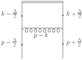
Figure 1: One-loop vertex diagram for the quark quasi-GPD.

In this Appendix, we present some technical details in calculating the following dimensionless integral that arises from the vertex diagram in Fig. 1:

$$I^{N}_{n}(x,\xi)=\int_{0}^{1}dy_{1}\int_{0}^{1-y_{1}}dy_{2}\frac{N(y_{1},y_{2})}{\left\{y_{1}y_{2}t^{\prime}+\left[x-1+(1-\xi)y_{1}+(1+\xi)y_{2}\right]^{2}\right\}^{n+\varepsilon}},$$ (70)

where $N$ is a function of Feynman parameters $y_{1}$ and $y_{2}$ and $n$ is the power of the denominator of the integrand; $t^{\prime}=-t/(p^{z})^{2}$. In unphysical regions ($x<-\xi$ and $x>1$), the integral has no $1/\varepsilon$ pole so that it can be easily calculated by setting $\varepsilon=0$. However, this is not the case in the Efremov-Radyushkin-Brodsky-Lepage (ERBL), $|x|<\xi$, and Dokshitzer-Gribov-Lipatov-Altarelli-Parisi (DGLAP), $\xi<x<1$, regions where there are IR divergences.

As an example, we evaluate the integral with $N=1$ and $n=3/2$. After integration over $y_{2}$, the remaining integrand denoted as $F(y_{1},\varepsilon)$ contains hypergeometric functions ${}_{2}F_{1}$. We identify the divergent part of $F(y_{1},\varepsilon)$ as $A(\varepsilon)/y_{1}^{1+\varepsilon}$ in the limit of $\varepsilon\to 0$, and then separate it out from the integral,

$$I^{1}_{3/2}(x,\xi)=\int_{0}^{1}dy_{1}\left[F(y_{1},\varepsilon)-\frac{A(\varepsilon)}{y_{1}^{1+\varepsilon}}\right]\bigg{|}_{\varepsilon\rightarrow 0}+\int_{0}^{1}dy_{1}\frac{A(\varepsilon)}{y_{1}^{1+\varepsilon}}\,,$$ (71)

where the first term is convergent so that we can set $\varepsilon=0$ before the integration. We suppress $x$, $\xi$, and $t^{\prime}$ dependences of $F$ and $A$ for simplicity.

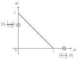
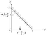
Figure 2: Integration in ERBL (left) and DGLAP (right) regions: The singularities are denoted by cross.

In Fig. 2, the singularities are shown in integration regions. We use Pfaff transformation to extract the divergent part

$${}_{2}F_{1}(a,b;c;z)=(1-z)^{-a}{}_{2}F_{1}(a,c-b;c;\frac{z}{z-1})\,.$$ (72)

We obtain

$$A(\varepsilon)=\frac{2}{t^{\prime}(x-1)}\left\{\begin{array}[]{lc}-1+2\varepsilon+\varepsilon\ln{\frac{t^{\prime}(1-x)}{4(1+\varepsilon)}}&|x|<\xi\\ -1+2\varepsilon+\varepsilon\ln{\frac{t^{\prime}(1-x)}{4(1+\varepsilon)}}-y_{1}^{1+\varepsilon}\left(1-2\varepsilon-2\varepsilon\ln(1-\xi)\right)\left|y_{1}-\frac{1-x}{1-\xi}\right|^{-1-2\varepsilon}&\xi<x<1\end{array}\right..$$ (75)

Finally, we have

$$I^{1}_{3/2}(x,\xi)=\left\{\begin{array}[]{lc}\frac{1}{2(1-x)(x^{2}-\xi^{2})}&x<-\xi\\ -\frac{2}{t^{\prime}(1-x)}\left[\frac{1}{\varepsilon}-2+\ln\frac{4(\xi-x)(1+\xi)^{2}}{t^{\prime}(1-x)^{2}(x+\xi)}\right]&|x|<\xi\\ -\frac{4}{t^{\prime}(1-x)}\left[\frac{1}{\varepsilon}-2+\ln\frac{4(1-\xi^{2})}{t^{\prime}(1-x)^{2}}\right]&\xi<x<1\\ -\frac{1}{2(1-x)(x^{2}-\xi^{2})}&x>1\end{array}\right..$$ (80)

More generally, when calculating the vertex diagram in Fig.(1), we encounter integrals similar to Eq.(70) with numerator of the integrand replaced by polynomials of $y_{1}$ and $y_{2}$. After integrating out $y_{2}$, we obtain Appell hypergeometric function $F_{1}$. In this case, to separate the divergent part, we need Euler transformation

$$F_{1}(\alpha;\beta,\beta^{\prime};\gamma;x,y)=(1-x)^{-\beta}(1-y)^{-\beta^{\prime}}F_{1}(\gamma-\alpha;\beta,\beta^{\prime};\gamma;\frac{x}{x-1},\frac{y}{y-1})\,.$$ (81)

In the following, we list integrals used in our calculation:

1. In unphysical region $x<-\xi$, there is no divergence.

   $$I^{1}_{1/2} =\frac{1-x}{1-\xi^{2}}\ln\left|\frac{1-x}{x-\xi}\right|+\frac{x+\xi}{2\xi(1+\xi)}\ln\left|\frac{x-\xi}{x+\xi}\right|\,,$$ (82)

   $$I^{y_{1}}_{3/2} =-\frac{1}{4\xi(1-\xi)(x-\xi)}+\frac{1}{2(1+\xi)(1-\xi)^{2}}\ln\left|\frac{1-x}{x-\xi}\right|+\frac{1}{8\xi^{2}(1+\xi)}\ln\left|\frac{x-\xi}{x+\xi}\right|\,,$$ (83)

   $$I^{y_{2}}_{3/2} =I^{y_{1}}_{3/2}\Big{|}_{\xi\rightarrow-\xi}\,,$$ (84)

   $$I^{y_{1}^{2}}_{3/2} =\frac{x-3x\xi+2\xi^{2}}{4\xi^{2}(x-\xi)(1-\xi)^{2}}+\frac{1-x}{(1+\xi)(1-\xi)^{3}}\ln\left|\frac{1-x}{x-\xi}\right|+\frac{\xi+x}{8\xi^{3}(1+\xi)}\ln\left|\frac{x-\xi}{x+\xi}\right|\,,$$ (85)

   $$I^{y_{2}^{2}}_{3/2} =I^{y_{1}^{2}}_{3/2}\Big{|}_{\xi\rightarrow-\xi}\,,$$ (86)

   $$I^{y_{1}y_{2}}_{3/2} =-\frac{1}{4\xi^{2}(1-\xi^{2})}+\frac{1-x}{2(1-\xi^{2})^{2}}\ln\left|\frac{1-x}{x-\xi}\right|-\frac{x+2x\xi+\xi^{2}}{8\xi^{3}(1+\xi)^{2}}\ln\left|\frac{x-\xi}{x+\xi}\right|.$$ (87)

2. In ERBL region $|x|<\xi$, $I^{y_{2}}_{3/2}$ and $I^{y_{2}^{2}}_{3/2}$ are divergent.

   $$I^{1}_{1/2} =\frac{x+\xi}{2\xi(1+\xi)}\ln\frac{16\xi^{2}}{t^{\prime}}+\frac{1-x}{1-\xi^{2}}\ln\frac{1+\xi}{2\xi}\,,$$ (88)

   $$I^{y_{1}}_{3/2} =-\frac{2}{t^{\prime}(1-\xi)}\ln\frac{(\xi-x)(1+\xi)}{2\xi(1-x)}\,,$$ (89)

   $$I^{y_{2}}_{3/2} =-\frac{2}{t^{\prime}(1+\xi)}\left[\frac{1}{\varepsilon}-2+\ln\frac{8\xi(1+\xi)}{t^{\prime}(1-x)(x+\xi)}\right]\,,$$ (90)

   $$I^{y_{1}^{2}}_{3/2} =-\frac{x+\xi}{t^{\prime}\xi(1-\xi)}+\frac{2(1-x)}{t^{\prime}(1-\xi)^{2}}\ln\frac{2\xi(1-x)}{(1+\xi)(\xi-x)}\,,$$ (91)

   $$I^{y_{2}^{2}}_{3/2} =-\frac{(1-\xi)(x+\xi)}{t^{\prime}\xi(1+\xi)^{2}}-\frac{2(1-x)}{t^{\prime}(1+\xi)^{2}}\left[\frac{1}{\varepsilon}-2+\ln\frac{8\xi(1+\xi)}{t^{\prime}(1-x)(x+\xi)}\right]\,,$$ (92)

   $$I^{y_{1}y_{2}}_{3/2} =\frac{x+\xi}{t^{\prime}\xi(1+\xi)}\,.$$ (93)

3. In DGLAP region $\xi<x<1$, $I^{y_{1}}_{3/2}$, $I^{y_{2}}_{3/2}$, $I^{y_{1}^{2}}_{3/2}$, and $I^{y_{2}^{2}}_{3/2}$ are divergent.

   $$I^{1}_{1/2} =\frac{x-\xi^{2}}{2\xi(1-\xi^{2})}\ln\frac{x+\xi}{x-\xi}+\frac{1-x}{1-\xi^{2}}\ln\frac{4(1-\xi^{2})\sqrt{x^{2}-\xi^{2}}}{t^{\prime}(1-x)}\,,$$ (94)

   $$I^{y_{1}}_{3/2} =\frac{1-x}{2(1-\xi)}I^{1}_{3/2}\,,$$ (95)

   $$I^{y_{2}}_{3/2} =\frac{1-x}{2(1+\xi)}I^{1}_{3/2}\,,$$ (96)

   $$I^{y_{1}^{2}}_{3/2} =\frac{(1-x)^{2}}{2(1-\xi)^{2}}I^{1}_{3/2}-\frac{2(1-x)}{t^{\prime}(1-\xi)^{2}}\,,$$ (97)

   $$I^{y_{2}^{2}}_{3/2} =\frac{(1-x)^{2}}{2(1+\xi)^{2}}I^{1}_{3/2}-\frac{2(1-x)}{t^{\prime}(1+\xi)^{2}}\,,$$ (98)

   $$I^{y_{1}y_{2}}_{3/2} =\frac{2(1-x)}{t^{\prime}(1-\xi^{2})}\,.$$ (99)

4. In unphysical region $x>1$, the integrals are the same as functions in another unphysical region but with an overall minus sign, $I^{P(y_{1},y_{2})}_{n}(x>1)=-I^{P(y_{1},y_{2})}_{n}(x<-\xi)$. See Eq. (80) for an example.

References

- Ji (2004) X. Ji, Ann. Rev. Nucl. Part. Sci. 54, 413 (2004).
- Diehl (2003) M. Diehl, Phys. Rept. 388, 41 (2003), arXiv:hep-ph/0307382 [hep-ph] .
- Belitsky and Radyushkin (2005) A. V. Belitsky and A. V. Radyushkin, Phys. Rept. 418, 1 (2005), arXiv:hep-ph/0504030 [hep-ph] .
- Adloff et al. (2001) C. Adloff et al. (H1), Phys. Lett. B517, 47 (2001), arXiv:hep-ex/0107005 [hep-ex] .
- Chekanov et al. (2003) S. Chekanov et al. (ZEUS), Phys. Lett. B573, 46 (2003), arXiv:hep-ex/0305028 [hep-ex] .
- Aktas et al. (2005) A. Aktas et al. (H1), Eur. Phys. J. C44, 1 (2005), arXiv:hep-ex/0505061 [hep-ex] .
- Airapetian et al. (2001) A. Airapetian et al. (HERMES), Phys. Rev. Lett. 87, 182001 (2001), arXiv:hep-ex/0106068 [hep-ex] .
- Airapetian et al. (2011) A. Airapetian et al. (HERMES), Phys. Lett. B704, 15 (2011), arXiv:1106.2990 [hep-ex] .
- Airapetian et al. (2012) A. Airapetian et al. (HERMES), JHEP 07, 032 (2012), arXiv:1203.6287 [hep-ex] .
- Gautheron et al. (2010) F. Gautheron et al. (COMPASS), (2010).
- Defurne et al. (2015) M. Defurne et al. (Jefferson Lab Hall A), Phys. Rev. C92, 055202 (2015), arXiv:1504.05453 [nucl-ex] .
- Jo et al. (2015) H. S. Jo et al. (CLAS), Phys. Rev. Lett. 115, 212003 (2015), arXiv:1504.02009 [hep-ex] .
- Seder et al. (2015) E. Seder et al. (CLAS), Phys. Rev. Lett. 114, 032001 (2015), [Addendum: Phys. Rev. Lett.114,no.8,089901(2015)], arXiv:1410.6615 [hep-ex] .
- Dudek et al. (2012) J. Dudek et al., Eur. Phys. J. A48, 187 (2012), arXiv:1208.1244 [hep-ex] .
- Accardi et al. (2016) A. Accardi et al., Eur. Phys. J. A52, 268 (2016), arXiv:1212.1701 [nucl-ex] .
- Aschenauer et al. (2014) E. C. Aschenauer et al., (2014), arXiv:1409.1633 [physics.acc-ph] .
- Chen (2018) X. Chen, Proceedings, 26th International Workshop on Deep Inelastic Scattering and Related Subjects (DIS 2018): Port Island, Kobe, Japan, April 16-20, 2018, PoS DIS2018, 170 (2018), arXiv:1809.00448 [nucl-ex] .
- Bacchetta (2016) A. Bacchetta, Eur. Phys. J. A52, 163 (2016).
- Hagler et al. (2003) P. Hagler, J. W. Negele, D. B. Renner, W. Schroers, T. Lippert, and K. Schilling (LHPC, SESAM), Phys. Rev. D68, 034505 (2003), arXiv:hep-lat/0304018 [hep-lat] .
- Gockeler et al. (2004) M. Gockeler, R. Horsley, D. Pleiter, P. E. L. Rakow, A. Schafer, G. Schierholz, and W. Schroers (QCDSF), Phys. Rev. Lett. 92, 042002 (2004), arXiv:hep-ph/0304249 [hep-ph] .
- Schroers et al. (2004) W. Schroers et al. (LHPC, SESAM), Lattice field theory. Proceedings, 21st International Symposium, Lattice 2003, Tsukuba, Japan, July 15-19, 2003, Nucl. Phys. Proc. Suppl. 129, 907 (2004), [,907(2003)], arXiv:hep-lat/0309065 [hep-lat] .
- Gockeler et al. (2005) M. Gockeler, P. Hagler, R. Horsley, D. Pleiter, P. E. L. Rakow, A. Schafer, G. Schierholz, and J. M. Zanotti (QCDSF, UKQCD), Phys. Lett. B627, 113 (2005), arXiv:hep-lat/0507001 [hep-lat] .
- Hagler et al. (2008) P. Hagler et al. (LHPC), Phys. Rev. D77, 094502 (2008), arXiv:0705.4295 [hep-lat] .
- Brommel et al. (2007) D. Brommel et al. (QCDSF-UKQCD), Proceedings, 25th International Symposium on Lattice field theory (Lattice 2007): Regensburg, Germany, July 30-August 4, 2007, PoS LATTICE2007, 158 (2007), arXiv:0710.1534 [hep-lat] .
- Alexandrou et al. (2011) C. Alexandrou, J. Carbonell, M. Constantinou, P. A. Harraud, P. Guichon, K. Jansen, C. Kallidonis, T. Korzec, and M. Papinutto, Phys. Rev. D83, 114513 (2011), arXiv:1104.1600 [hep-lat] .
- Ji (2013) X. Ji, Phys. Rev. Lett. 110, 262002 (2013), arXiv:1305.1539 [hep-ph] .
- Ji (2014) X. Ji, Sci. China Phys. Mech. Astron. 57, 1407 (2014), arXiv:1404.6680 [hep-ph] .
- Ji et al. (2015a) X. Ji, A. Schäfer, X. Xiong, and J.-H. Zhang, Phys. Rev. D92, 014039 (2015a), arXiv:1506.00248 [hep-ph] .
- Xiong and Zhang (2015) X. Xiong and J.-H. Zhang, Phys. Rev. D92, 054037 (2015), arXiv:1509.08016 [hep-ph] .
- Xiong et al. (2014) X. Xiong, X. Ji, J.-H. Zhang, and Y. Zhao, Phys. Rev. D90, 014051 (2014), arXiv:1310.7471 [hep-ph] .
- Ji and Zhang (2015) X. Ji and J.-H. Zhang, Phys. Rev. D92, 034006 (2015), arXiv:1505.07699 [hep-ph] .
- Li (2016) H.-n. Li, Phys. Rev. D94, 074036 (2016), arXiv:1602.07575 [hep-ph] .
- Chen et al. (2016) J.-W. Chen, S. D. Cohen, X. Ji, H.-W. Lin, and J.-H. Zhang, Nucl. Phys. B911, 246 (2016), arXiv:1603.06664 [hep-ph] .
- Ishikawa et al. (2016) T. Ishikawa, Y.-Q. Ma, J.-W. Qiu, and S. Yoshida, (2016), arXiv:1609.02018 [hep-lat] .
- Chen et al. (2017a) J.-W. Chen, X. Ji, and J.-H. Zhang, Nucl. Phys. B915, 1 (2017a), arXiv:1609.08102 [hep-ph] .
- Monahan and Orginos (2017) C. Monahan and K. Orginos, JHEP 03, 116 (2017), arXiv:1612.01584 [hep-lat] .
- Radyushkin (2017) A. Radyushkin, Phys. Lett. B767, 314 (2017), arXiv:1612.05170 [hep-ph] .
- Zhang et al. (2017) J.-H. Zhang, J.-W. Chen, X. Ji, L. Jin, and H.-W. Lin, Phys. Rev. D95, 094514 (2017), arXiv:1702.00008 [hep-lat] .
- Carlson and Freid (2017) C. E. Carlson and M. Freid, Phys. Rev. D95, 094504 (2017), arXiv:1702.05775 [hep-ph] .
- Ishikawa et al. (2017) T. Ishikawa, Y.-Q. Ma, J.-W. Qiu, and S. Yoshida, Phys. Rev. D96, 094019 (2017), arXiv:1707.03107 [hep-ph] .
- Xiong et al. (2017) X. Xiong, T. Luu, and U.-G. Meißner, (2017), arXiv:1705.00246 [hep-ph] .
- Constantinou and Panagopoulos (2017) M. Constantinou and H. Panagopoulos, Phys. Rev. D96, 054506 (2017), arXiv:1705.11193 [hep-lat] .
- Ji et al. (2018a) X. Ji, J.-H. Zhang, and Y. Zhao, Phys. Rev. Lett. 120, 112001 (2018a), arXiv:1706.08962 [hep-ph] .
- Green et al. (2018) J. Green, K. Jansen, and F. Steffens, Phys. Rev. Lett. 121, 022004 (2018), arXiv:1707.07152 [hep-lat] .
- Chen et al. (2018a) J.-W. Chen, T. Ishikawa, L. Jin, H.-W. Lin, Y.-B. Yang, J.-H. Zhang, and Y. Zhao, Phys. Rev. D97, 014505 (2018a), arXiv:1706.01295 [hep-lat] .
- Alexandrou et al. (2017a) C. Alexandrou, K. Cichy, M. Constantinou, K. Hadjiyiannakou, K. Jansen, H. Panagopoulos, and F. Steffens, Nucl. Phys. B923, 394 (2017a), arXiv:1706.00265 [hep-lat] .
- Chen et al. (2017b) J.-W. Chen, T. Ishikawa, L. Jin, H.-W. Lin, Y.-B. Yang, J.-H. Zhang, and Y. Zhao, (2017b), arXiv:1710.01089 [hep-lat] .
- Lin et al. (2018a) H.-W. Lin, J.-W. Chen, T. Ishikawa, and J.-H. Zhang (LP3), Phys. Rev. D98, 054504 (2018a), arXiv:1708.05301 [hep-lat] .
- Chen et al. (2017c) J.-W. Chen, T. Ishikawa, L. Jin, H.-W. Lin, A. Schäfer, Y.-B. Yang, J.-H. Zhang, and Y. Zhao, (2017c), arXiv:1711.07858 [hep-ph] .
- Rossi and Testa (2017) G. C. Rossi and M. Testa, Phys. Rev. D96, 014507 (2017), arXiv:1706.04428 [hep-lat] .
- Ji et al. (2017) X. Ji, J.-H. Zhang, and Y. Zhao, Nucl. Phys. B924, 366 (2017), arXiv:1706.07416 [hep-ph] .
- Hobbs (2018) T. J. Hobbs, Phys. Rev. D97, 054028 (2018), arXiv:1708.05463 [hep-ph] .
- Jia et al. (2017) Y. Jia, S. Liang, L. Li, and X. Xiong, JHEP 11, 151 (2017), arXiv:1708.09379 [hep-ph] .
- Wang et al. (2018) W. Wang, S. Zhao, and R. Zhu, Eur. Phys. J. C78, 147 (2018), arXiv:1708.02458 [hep-ph] .
- Stewart and Zhao (2018) I. W. Stewart and Y. Zhao, Phys. Rev. D97, 054512 (2018), arXiv:1709.04933 [hep-ph] .
- Monahan (2018) C. Monahan, Phys. Rev. D97, 054507 (2018), arXiv:1710.04607 [hep-lat] .
- Wang and Zhao (2018) W. Wang and S. Zhao, JHEP 05, 142 (2018), arXiv:1712.09247 [hep-ph] .
- Izubuchi et al. (2018) T. Izubuchi, X. Ji, L. Jin, I. W. Stewart, and Y. Zhao, Phys. Rev. D98, 056004 (2018), arXiv:1801.03917 [hep-ph] .
- Xu et al. (2018a) J. Xu, Q.-A. Zhang, and S. Zhao, Phys. Rev. D97, 114026 (2018a), arXiv:1804.01042 [hep-ph] .
- Briceño et al. (2018) R. A. Briceño, J. V. Guerrero, M. T. Hansen, and C. J. Monahan, Phys. Rev. D98, 014511 (2018), arXiv:1805.01034 [hep-lat] .
- Xu et al. (2018b) S.-S. Xu, L. Chang, C. D. Roberts, and H.-S. Zong, Phys. Rev. D97, 094014 (2018b), arXiv:1802.09552 [nucl-th] .
- Jia et al. (2018) Y. Jia, S. Liang, X. Xiong, and R. Yu, Phys. Rev. D98, 054011 (2018), arXiv:1804.04644 [hep-th] .
- Spanoudes and Panagopoulos (2018) G. Spanoudes and H. Panagopoulos, Phys. Rev. D98, 014509 (2018), arXiv:1805.01164 [hep-lat] .
- Rossi and Testa (2018) G. Rossi and M. Testa, Phys. Rev. D98, 054028 (2018), arXiv:1806.00808 [hep-lat] .
- Liu et al. (2018a) Y.-S. Liu, J.-W. Chen, L. Jin, H.-W. Lin, Y.-B. Yang, J.-H. Zhang, and Y. Zhao, (2018a), arXiv:1807.06566 [hep-lat] .
- Ji et al. (2018b) X. Ji, Y. Liu, and I. Zahed, (2018b), arXiv:1807.07528 [hep-ph] .
- Bhattacharya et al. (2019) S. Bhattacharya, C. Cocuzza, and A. Metz, Phys. Lett. B788, 453 (2019), arXiv:1808.01437 [hep-ph] .
- Radyushkin (2019) A. V. Radyushkin, Phys. Lett. B788, 380 (2019), arXiv:1807.07509 [hep-ph] .
- Zhang et al. (2018) J.-H. Zhang, X. Ji, A. Schäfer, W. Wang, and S. Zhao, (2018), arXiv:1808.10824 [hep-ph] .
- Li et al. (2018) Z.-Y. Li, Y.-Q. Ma, and J.-W. Qiu, (2018), arXiv:1809.01836 [hep-ph] .
- Braun et al. (2018) V. M. Braun, A. Vladimirov, and J.-H. Zhang, (2018), arXiv:1810.00048 [hep-ph] .
- Lin et al. (2015) H.-W. Lin, J.-W. Chen, S. D. Cohen, and X. Ji, Phys. Rev. D91, 054510 (2015), arXiv:1402.1462 [hep-ph] .
- Alexandrou et al. (2015) C. Alexandrou, K. Cichy, V. Drach, E. Garcia-Ramos, K. Hadjiyiannakou, K. Jansen, F. Steffens, and C. Wiese, Phys. Rev. D92, 014502 (2015), arXiv:1504.07455 [hep-lat] .
- Alexandrou et al. (2017b) C. Alexandrou, K. Cichy, M. Constantinou, K. Hadjiyiannakou, K. Jansen, F. Steffens, and C. Wiese, Phys. Rev. D96, 014513 (2017b), arXiv:1610.03689 [hep-lat] .
- Chen et al. (2017d) J.-W. Chen, L. Jin, H.-W. Lin, A. Schäfer, P. Sun, Y.-B. Yang, J.-H. Zhang, R. Zhang, and Y. Zhao, (2017d), arXiv:1712.10025 [hep-ph] .
- Alexandrou et al. (2018a) C. Alexandrou, K. Cichy, M. Constantinou, K. Jansen, A. Scapellato, and F. Steffens, Phys. Rev. Lett. 121, 112001 (2018a), arXiv:1803.02685 [hep-lat] .
- Chen et al. (2018b) J.-W. Chen, L. Jin, H.-W. Lin, Y.-S. Liu, Y.-B. Yang, J.-H. Zhang, and Y. Zhao, (2018b), arXiv:1803.04393 [hep-lat] .
- Chen et al. (2018c) J.-W. Chen, L. Jin, H.-W. Lin, Y.-S. Liu, A. Schäfer, Y.-B. Yang, J.-H. Zhang, and Y. Zhao, (2018c), arXiv:1804.01483 [hep-lat] .
- Alexandrou et al. (2018b) C. Alexandrou, K. Cichy, M. Constantinou, K. Jansen, A. Scapellato, and F. Steffens, Phys. Rev. D98, 091503 (2018b), arXiv:1807.00232 [hep-lat] .
- Lin et al. (2018b) H.-W. Lin, J.-W. Chen, L. Jin, Y.-S. Liu, Y.-B. Yang, J.-H. Zhang, and Y. Zhao, (2018b), arXiv:1807.07431 [hep-lat] .
- Fan et al. (2018) Z.-Y. Fan, Y.-B. Yang, A. Anthony, H.-W. Lin, and K.-F. Liu, Phys. Rev. Lett. 121, 242001 (2018), arXiv:1808.02077 [hep-lat] .
- Liu et al. (2018b) Y.-S. Liu, J.-W. Chen, L. Jin, R. Li, H.-W. Lin, Y.-B. Yang, J.-H. Zhang, and Y. Zhao, (2018b), arXiv:1810.05043 [hep-lat] .
- Ji et al. (2015b) X. Ji, P. Sun, X. Xiong, and F. Yuan, Phys. Rev. D91, 074009 (2015b), arXiv:1405.7640 [hep-ph] .
- Ji et al. (2018c) X. Ji, L.-C. Jin, F. Yuan, J.-H. Zhang, and Y. Zhao, (2018c), arXiv:1801.05930 [hep-ph] .
- Ebert et al. (2019a) M. A. Ebert, I. W. Stewart, and Y. Zhao, Phys. Rev. D99, 034505 (2019a), arXiv:1811.00026 [hep-ph] .
- Constantinou et al. (2019) M. Constantinou, H. Panagopoulos, and G. Spanoudes, (2019), arXiv:1901.03862 [hep-lat] .
- Ebert et al. (2019b) M. A. Ebert, I. W. Stewart, and Y. Zhao, (2019b), arXiv:1901.03685 [hep-ph] .
- Martinelli et al. (1995) G. Martinelli, C. Pittori, C. T. Sachrajda, M. Testa, and A. Vladikas, Nucl. Phys. B445, 81 (1995), arXiv:hep-lat/9411010 [hep-lat] .
- Dulat et al. (2016) S. Dulat, T.-J. Hou, J. Gao, M. Guzzi, J. Huston, P. Nadolsky, J. Pumplin, C. Schmidt, D. Stump, and C. P. Yuan, Phys. Rev. D93, 033006 (2016), arXiv:1506.07443 [hep-ph] .
- Ball et al. (2017) R. D. Ball et al. (NNPDF), Eur. Phys. J. C77, 663 (2017), arXiv:1706.00428 [hep-ph] .
- Harland-Lang et al. (2015) L. A. Harland-Lang, A. D. Martin, P. Motylinski, and R. S. Thorne, Eur. Phys. J. C75, 204 (2015), arXiv:1412.3989 [hep-ph] .
- Nocera et al. (2014) E. R. Nocera, R. D. Ball, S. Forte, G. Ridolfi, and J. Rojo (NNPDF), Nucl. Phys. B887, 276 (2014), arXiv:1406.5539 [hep-ph] .
- Ethier et al. (2017) J. J. Ethier, N. Sato, and W. Melnitchouk, Phys. Rev. Lett. 119, 132001 (2017), arXiv:1705.05889 [hep-ph] .
- Ma and Qiu (2018) Y.-Q. Ma and J.-W. Qiu, Phys. Rev. Lett. 120, 022003 (2018), arXiv:1709.03018 [hep-ph] .
- Wang et al. (2019) W. Wang, J.-H. Zhang, S. Zhao, and R. Zhu, (2019), arXiv:1904.00978 [hep-ph] .
- Braun et al. (2003) V. M. Braun, G. P. Korchemsky, and D. Mueller, Prog. Part. Nucl. Phys. 51, 311 (2003), arXiv:hep-ph/0306057 [hep-ph] .
- Efremov and Radyushkin (1980) A. V. Efremov and A. V. Radyushkin, Theor. Math. Phys. 42, 97 (1980), [Teor. Mat. Fiz.42,147(1980)].
- Mueller (1994) D. Mueller, Phys. Rev. D49, 2525 (1994).
- Braun and Mueller (2008) V. Braun and D. Mueller, Eur. Phys. J. C55, 349 (2008), arXiv:0709.1348 [hep-ph] .
- Müller et al. (1994) D. Müller, D. Robaschik, B. Geyer, F. M. Dittes, and J. Ho?ejši, Fortsch. Phys. 42, 101 (1994), arXiv:hep-ph/9812448 [hep-ph] .
- Ji (1997) X.-D. Ji, Phys. Rev. D55, 7114 (1997), arXiv:hep-ph/9609381 [hep-ph] .
- Liu et al. (2018c) Y.-S. Liu, W. Wang, J. Xu, Q.-A. Zhang, S. Zhao, and Y. Zhao, (2018c), arXiv:1810.10879 [hep-ph] .
- Meissner et al. (2007) S. Meissner, A. Metz, and K. Goeke, Phys. Rev. D76, 034002 (2007), arXiv:hep-ph/0703176 [HEP-PH] .
- Braun et al. (2004) V. M. Braun, E. Gardi, and S. Gottwald, Nucl. Phys. B685, 171 (2004), arXiv:hep-ph/0401158 [hep-ph] .