Binary phase separation in a collection of self-propelled particle with variable speed

Abstract

We study the collective behavior of binary mixture of self-propelled particles. Particles moves along their heading direction with variable speed and interact through short range alignment interaction. A variable speed parameter $\gamma>0$ is introduced such that for $\gamma=0.0$ model reduces to constant speed Vicsek’s model. We mix the particles with two different $\gamma$’s and study the steady state behavior of the mixture for different choice of $\gamma$’s and noise strength. One of the $\gamma$ is kept fixed to $1.0$ and another one is varied from small $0.0$ to larger values $8.0$. Properties of system is characterise by two types of order parameters (i) orientation order parameter, which is a measure of ordering in the system and (ii) density order parameter, which measures the phase separation is the system. For all set of $\gamma$’s, system shows a transition from disorder-to-ordered state on the variation of noise strength. The nature of transition and critical noise is independent of value of $\gamma$, which is also supported from coarse-grained hydrodynamic study. On the variation of system parameters, ($\gamma$’s, $\eta$), we find four distinct phases, (i) ordered phase separated, (ii) ordered mixed, (iii) disordered mixed and (iv) disordered phase segragated. Our study shade light on different phases of mixture of different types of active particles.

I Introduction

Collection of polar self-propelled particle ubiquitous physicstoday ; fishschool . Examples ranges from very small intracellular scale to much larger scale sriramrev3 ; sriramrev2 ; sriramrev1 ; harada ; badoual ; nedelec ; rauch ; ben ; appleby ; helbing ; helbing1 ; physicstoday ; kuusela ; hubbard ; schaller ; sumino ; peruani ; bacterialcolonies . Study of such system started with the novel work of T. Vicsek vicsek , In this study, each individuals are modeled as point particle move along their heading direction with a constant speed and align through a short range alignment interaction with their neighbors. Interestingly different variants of Vicsek’s model is studied but mainly with constant speed chatepre2008 ; chate2007 ; katz ; shradhasudipta ; shradhamanna . But in reality there is no reason for the speed of particles to be fixed. For examples in everyday traffic, car can not move if stuck in jam situation but move freely, when other vehicles are moving in the same direction. Not only in everyday traffic but experiments on living bacteria Bacillus Subtilis observed that speed of each individual depends on polarisation of their neighbors goldstein2012pre . Our previous study is motivated by an experiment on fish school: and a variable speed model is introduced in shradhapre2012 . A variable speed model is introduced, where speed of the particle depends on their local neighbors orientation through a variable speed parameter $\gamma>0$ (with a power-law). For any $\gamma>0$ when particle moves in well ordered region then its speed is maximum and in the disordered region speed is close to zero. For $\gamma=0$, all the particle moves with constant speed. Hence model is very much applicable for situations where random moving crowd restrict the motion of particle. The variable speed parameter $\gamma$ introduced here can be thought of as characteristics of particles, which gives how particle response to its neighbors. It can have origin from various biological or physical factors. In this article we will not go into details of such factors. We will strictly consider a variable speed model introduced in shradhapre2012 . And ask the question what happens if we mix the particles with two different values of variable speed parameters ($\gamma_{1},\gamma_{2}$)? Whether we find a phase separation for certain range of system parameters, viz. noise strength and $\gamma$.
In this study one of the $\gamma_{1}=1$ is fixed, i.e. speed of the particle linearly vary with local neighbor’s alignment. And other $\gamma_{2}$ is tuned from $0$ to $8$. Experiment on fish-school (Golden-shiner) found that speed of the fish depends on local neighbor’s alignment with variable speed parameter $\gamma=6$ shradhapre2012 . Hence we expect for other type particle one will have different $\gamma$. Properties of the system is characterise by two types of order parameter. (a) orientation order parameter (OOP) $\chi$, which is a measure of global orientation of the flock and (b) density order parameter (DOP) $\phi$, which is measure of phase separation among two-types of particles. We first measure the $\chi$ as a function of noise strength for different values of variable speed parameter $\gamma_{2}$. For set of $\gamma$’s = ($\gamma_{1}=1,\gamma_{2}=0-8)$ we find a transition from disordered-to-ordered state on the variation of noise strength, critical noise (is close to $0.6$) is almost independent of the variable speed parameter $\gamma$. Which is further confirmed by the mean-field analysis of the coarse-grained hydrodynamic equations of motion for slow variables. On the variation of two parameter ($\gamma_{1},\gamma_{2})$ and noise strength we find four distinct phases. (i) For small noise when system is globally ordered $\chi\simeq 1$ and $\gamma_{2}>3$: the particles with two different $\gamma$’s are phase separated and $\phi>0.6$. Hence they move in the group of their own types of particles. Typical snapshot for small $\eta=0.2$ and $\gamma_{2}=8$ is shown in Fig. 1 (b) and (b’). We call this phase as ordered-phase separated phase (OPS). (ii) Again for small noise when $\chi$ is large but $\gamma_{2}$ is close to $\gamma_{1}=1$, phase separation decreases $\phi<0.6$. This is defined as ordered mixed phase (OM). Please see the snapshot Fig. 1(c) and (c’). As we increase noise strength and cross the ordered region $\eta>0.6$, we again find two different phase (iii) disorder mixed (DM) and disordered phase segregated (DPS) when difference is two $\gamma$’s is smaller/larger that $2$. Please see the snapshot shown in Fig. 1(d-e) and (d’-e’). In Fig. 3 we plot the DOP vs. $\gamma_{2}$ for two different noise strengths (a) $\eta=0.2$ in the ordered region and (b) $\eta=0.62$ in the disordered region. We draw the four phases with different shaded regions. Which shows the value of DOP for four distinct phase we find here. In rest of the article we discuss the four phases in detail and also compare the result with hydrodynamic equations of motion.
Rest of the article is divided in following manner. In section II we discuss our model and numerical details of the simulation. Section III contains the result of numerical study and in section V and VI we compare the result with coarse-grained hydrodynamic equations of motion and finally section IV concludes the results and shows final outcome of our study.

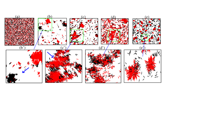
6

Figure 1: (color online) Top panel: real space snapshot of particle position of two types of particle with the direction of their velocity vector. Color represents two types particle. Black is for particle of type one and red for second type particle. (a) is for initial random homogeneous mixed state, (b) is for ordered phase separated state ($\gamma_{2}=8$, $\eta=0.2$), (c) ordered mixed ($\gamma_{2}=0.5$ $\eta=0.2$, (d) is for disordered mixed $(\gamma_{2}=0.5$, $\eta=0.62$) and (e) is for disordered phase segregated phase ($\gamma_{2}=8$, $\eta=0.62$). Bottom panel (b’-e’) are the zoomed version of top panel plot for better clarity of four different phases. All snapshots are collected in the steady state and plots are a part of full system. Other parameters are same as given in Fig. 1.

II Model

In our model, system consist of symmetric binary mixture of $N-$ point particles moving on a two-dimensional substrate. Each particle is defined by its position $r_{i}(t)$, velocity vector $v_{i}(t)$. The velocity of the particle is defined by its unit direction or orientation ${\bf n}_{i}(t)=(\cos(\theta_{i}(t)),\sin(\theta_{i}(t))$ and speed $v_{i}(t)$. The particles interact through a short range alignment interaction. Self-propulsion is introduced as a motion towards its orientation with a variable speed ($v_{i}(t)$ in unit time). Unlike the previous models vicsek ; chatepre2008 , here the speed of the particle depends on its neighbors. Hence a variable speed model is introduced shradhapre2012 . We first update the position of the particle

$$r_{i}(t+1)=r_{i}(t)+v_{i}(t){\bf n_{i}}(t)$$ (1)

and the orientation update equation with a short range alignment interaction

$${\bf n_{i}}(t+1)=\frac{\sum_{j\in R_{0}}{\bf n_{j}}(t)+N_{i}(t){\bf\eta}_{i}}{W_{i}(t)}$$ (2)

where in the nominator sum is over all the particles within the interaction radius $R_{0}$ of the $i^{th}$ particle, i.e., $|{\bf r}_{j}(t)-{\bf r}_{i}(t)|<R_{0}$ . $N_{i}(t)$ is the number of particles within the interaction radius of the $i^{th}$ particle at time $t$. $W_{i}(t)$ is the normalisation factor, which make the R. H. S. of Eq. 2 again a unit vector. The strength of the noise $\eta$ is varied between $0$ to $1$. for $v_{i}(t)=v_{0}$ model is similar to Vicsek model vicsek . But here unlike the Vicsek’s model: we introduce the variable speed: guided by the experiments on fish-school, in shradhapre2012 a variable speed model is introduced by considering a simple power-law relationship between the local polarisation $\chi_{i}(t)$ around $i^{th}$ particle with speed $v_{i}(t)$ such that.

$$v_{i}(t)=v_{(\chi_{i}(t))^{\gamma}}$$ (3)

where

$${\chi_{i}}(t)=|\frac{\sum_{j\in R_{0}}{\bf n_{j}}(t)}{N_{i}(t)}|$$ (4)

and $\gamma$, is variable speed parameter such that particle moves with maximum speed $v_{0}$ in well ordered region and almost static (zero speed) in completely disordered region. For $\gamma=0$, model reduces to constant speed. Note that for any $\gamma$ an isolated particle will move with maximal speed $v_{0}$. Hence, the variable speed parameter $\gamma$ controls the shape of curve that relates local order and speed. For $\gamma=1$, local speed vary linearly with local polarisation.
Here we consider a binary mixture of particles by introducing two parameters ($\gamma_{1}$ and $\gamma_{2}$ ) of speed such that $v^{i}_{1}(t)=v_{0}{(\chi(t))^{\gamma_{1}}}$ and $v^{i}_{2}(t)=v_{0}{(\chi(t))^{\gamma_{2}}}$. One of the $\gamma$, $\gamma_{1}$ is fixed to $1.0$ and these particles are called as type one and other $\gamma_{2}$ is varied from $(0,8)$ and particles are called type two. Agent based numerical simulation is performed with $N_{1}$ particles of type one and $N_{2}$ particles of type two ($N_{1}=N_{2}=N/2$). Started with random mixed state of both types particles, all the particles are sequentially updated using the above Eqs. 1,2,3 And it is counted as one simulation step. Simulations are performed for $10^{7}$ simulation steps with $L=100$ for different values of $\gamma_{2}=(0,8)$ and noise strength $\eta$. Density of particle is fixed to $\rho=\frac{N}{L^{2}}$ and maximum speed of the particle $v_{0}=0.5$. For better quality of five different initial realisations are used.
We study the system for different set of $(\gamma_{2},\eta)$. Steady state is characterised by two types of order parameters: (i) orientation order parameter $\chi(t)=|\frac{1}{N}\sum_{i=1}^{N}{\bf{n}}_{i}(t)|.$, which is measure of orientation of all the particles. When $\chi(t)\simeq 1$ means the ordered state such that large number of particle moving in the same direction showing the collective motion. If $\chi(t)=0$ i.e. all the particle moving randomally in random direction (Disorder).
and density order parameter (DOP) $\phi=\frac{\sum_{i=1}^{N}|{\rho^{i}_{1}(t)}-{\rho^{i}_{2}(t)|}}{{\sum_{i=1}^{N}|{\rho^{i}_{1}(t)}+{\rho^{i}_{2}(t)|}}}$, which is a measure of phase separation among two types of particles, where $\rho^{i}_{k=1,2}(t)$ are the number of particle of type $k$ within the coarse-grained radius of $i^{th}$ particle of same type. The value of $\phi$ also lies between $0$ and $1$. when $\phi$ close to $1$, implies only same kind of particle inside the interaction radius. Which is possible when particles are phase separated. When $\phi$ is small, hence both types of particles present inside the interaction radius hence mixing.

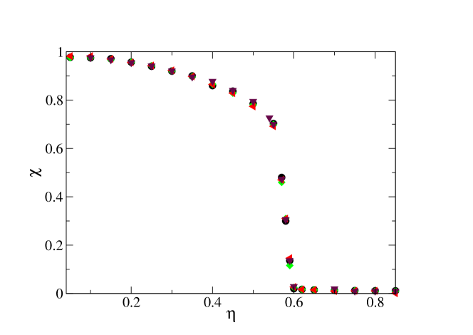
6

Figure 2: (color online) Plot of orientation order parameter (OOP) vs. noise strength $\eta$, $\gamma_{1}=1$, different curves are for different $\gamma_{2}$. $\circ$, $\square$, $\diamond$ and $\bigtriangleup$ are for $\gamma_{2}=2,4,6$ and 0.5 respectively. All the curves are independent of $\gamma_{2}$ and shows a transition from ordered state for small $\eta$ to disorder state for large $\eta$. Critical noise lies between $0.57-0.60$. Data is obtained for system size $L=100$ and simulation time $10^{7}$ in the steady state. Averaging is done over five independent realisations.

III Results

We first calculate the mean value of $OOP$, $\chi$, averaged over time in the steady state and over many realisations. In Fig. 2 we plot the steady state $\chi$ vs. $\eta$ for different $\gamma_{2}$. For all set of $\gamma_{2}$ we find a transition from disordered random state to ordered state when $\eta$ is tuned from large to smaller values. For all set of $\gamma_{2}$ transition remains the same. Hence disorder-to-order transition is independent of variable speed parameter $\gamma$. Which is further given in section V using the coarse-grained hydrodynamic equations of motion for slow variables. We also calculate mean value of $DOP$ $\phi$, where definition of “mean” is same as defined before. When the $DOP\simeq 1$, then two species are phase separated from each other and when DOP is small then they are mixed. Now we find four types of phases in terms of the two order parameters ($\chi,\phi$), (a) ordered phase separated (OPS), (b) ordered mixed (OM), (c) disordered mixed (DM) and (d) disordered phase segregated (DPS). In Fig. 1 we plot the four snapshots for four combination of ($\eta,\gamma_{2}$). Since for all $\gamma_{2}$ disorder-to-order transition happens at same $\eta$. Hence all of our later measurements are strictly restricted to ordered $\eta<0.4$ and disordered state $\eta>0.6$. Properties near to the disorder-to-order transition is also interesting but it is not of our interest in this work. For small $\eta=0.2$ and larger $\gamma_{2}>3$, we find $OOP$, $\chi\simeq 1$ and also $\phi\simeq 1$, hence in the steady state particles form ordered clusters and also phase separated. Typical snapshot for this kind of phase is shown in Fig. 1(b) and (b’). We name it as order phase separated phase (OPS). As we decreases the $\gamma_{2}$ then the difference in the speed of two types of particle decreases and they start to mix. Fig. 1(c) and (c’) shows one of the typical snapshot of such phase. We call such phase as order mixed phase (OM). In this phase $\chi$ is still close to $1$ but $\phi<0.6$. Now as we go to the disordered state $\eta=0.65$ and vary $\gamma_{2}$. For small $\gamma_{2}<3$, the two types of particles are always mixed and we find no phase separation. Both $\phi$ and $\chi$ is small, We call this phase as disorder mixed (DM) and for large $\gamma_{2}>3$, we find disorder-phase segregated phase (DPS). The two order parameters $OOP$ and $DOP$ behave similarly for the above two phases but they differ in detail. Which we will explain in following subsections. Typical snapshot of the two phases are shown in Fig.1 (d-e) and (d’-e’) respectively.
Now we will briefly explain characteristic of all four phases in detail.

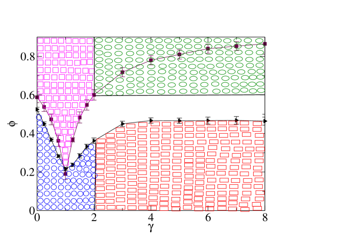
6

Figure 3: (color online): Plot of DOP vs. $\gamma_{2}$ for two different $\eta=0.2$ ($\circ$) and $0.62$ ($\square$). Other parameters are same as defined in Fig. 1. Different shaded regions represents the four different phases in the system. (i) Green ellipses represents OPS for ($2<\gamma_{2}$, $\eta<0.5$). (ii) Magenta square shows OM phase ($0<\gamma_{2}<2$, $\eta<0.5$). (iii) Blue circles region represents DM phase for $\eta>0.6$ and $0<\gamma_{2}<2$ and (iv) Red rectangles for DPS phase for ($2<\gamma_{2}$, $\eta>0.6$). Empty regions are near to the disorder-to-order phase and phase separation transition, which is not explored in detail in current work.

III.1 Ordered phase separated: OPS

For $\eta<0.4$ and large $\gamma_{2}$, the two order parameters $OOP$ and $DOP$ are close to $1$. In Fig.3 we plot the $DOP$ vs. $\gamma_{2}$ for two different $\eta=(0.2,0.62)$ values. For small $\eta=0.2$, starting from initially random and mixed state in the steady state, both types of particles forms moving clusters but they move in different clusters. For larger $\gamma_{2}$ and smaller $\eta$, clusters are more separated and as we increase $\eta$ and decrease $\gamma_{2}$ phase separation decreases as shown in Fig. 3. To further understand such phase separation we calculate the probability distribution function (PDF) of particle speed $P(v)$ for two types of particles. In Fig.4(a) we plot the $P(v)$ for both types of particle for different values of $\gamma_{2}=8$ and $\gamma_{1}=1$ and for noise strength $\eta=0.2$. $P(v)$ for both types of particle show one small peak at maximum possible speed $v=0.5$, which is mainly due to random moving particles. Another peak is present at smaller speed value $v<0.5$. This is contribution from clusters and it fits well with normal distribution (lines are fit to the Gaussian distribution). We find that the difference in the two peak position $\Delta v/v_{0}$ increases as we increase $\gamma_{2}$. Peak position represent the mean speed of particles inside the cluster. In Fig. 6 we plot $\Delta v/v_{0}$ vs. $\gamma_{2}$ for $\eta=0.2$.
In section VI we show the linearised study of coarse-grained hydrodynamic equations of motion for density of two types of particles and polarisation ordered parameter. The equations are studied for small fluctuations about homogeneous ordered state for different value of $\gamma_{2}$. We find that homogeneous ordered state is unstable for large $\gamma_{2}$, which further supports our numerical result. Which shows the presence of OPS state for large $\gamma_{2}$ and small $\eta$.
To further characterise different phases we calculate $P_{ij}(n)$, where $(i,j=1,2)$ and $n$ is number of particle. Since the two types of particles are phase separated in OPS, hence the two distributions $P_{12}(n)$ and $P_{21}(n)$ looks similar, and should show sharp decay for large $n$, which is due to less mixing of two types of particles. Other two distributions $P_{11}(n)$ and $P_{22}(n)$ have broad distribution which confirms the clustering of same types of particles. Please see the Fig. 5(a). In the lower panel of Fig. 5(a) we plot the $P_{ij}(n)$ on $\log-\log$ scale. Which shows that the tail of $P_{12}(n)$ $P_{21}(n)$ fits well with power $n^{-\alpha}$ with exponent $\alpha\simeq 2$, but $P_{11}(n)$ and $P_{22}(n)$ are better fitted with $\exp^{(\frac{-n}{n_{0}})}$ and $n_{0}\simeq 40$.

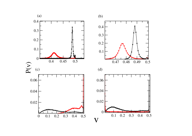
Figure 4: Plot of PDF of speed $P(v)$ vs. $v$ for four different phases (a-d) for OPS, OM, DM and DPS respectively. The two curves are for $P(v)$ for two types of particles. Symbols have same meaning as in Fig. 7. For all plots there is always a peak at maximum speed $v=v_{0}=0.5$ and second peak is at smaller value. The difference in two peak position is large for large $\gamma_{2}$ in ordered state. Other parameters are same as in Fig.2

III.2 ordered mixed: OM

In this phase as defined before orientation of particles are aligned along some mean direction hence $OOP$ is close to $1$, but both types of particles remain mix and a cluster consist of both types of particles as shown in Fig. 1(c) and (c’), hence $DOP<0.6$. In Fig. 4(b) we plot the $P(v)$ for $\gamma_{2}=0.5$ and $\eta=0.2$. We notice two features in the $P(v)$, one peak at $v_{0}=0.5$ which is again due to the random isolated moving particles. Second peak appears at $v_{0}<0.5$ for both types of particle. In comparison to previous case when difference in two $\gamma$’s $\gamma_{2}-\gamma_{1}$ is large, now difference in the two peak position decreases also the two distributions starts to overlap as shown in Fig. 4(b). The overlap between the distributions due to large number of particles of both types moving with same speed. Hence they belongs to the same cluster. Again we plot the the four $P_{ij}(n)$ in Fig. 5, all four $P_{ij}(n)$ decay exponentially with $n_{0}\approx 20-30$, which implies formation of large clusters. All four distributions are similar, hence one type of particle can be in the neighborhood of other type and also of the same type with equal probability. Which again confirms the mixed phase.

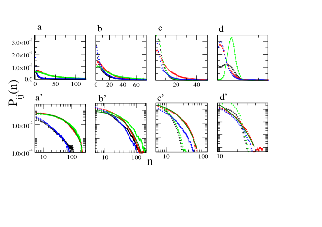
Figure 5: (color online): Plot of particle number PDF $P_{ij}(n)$ for four different phases OPS, OM, DM and DPS, (a-d) respectively. Top panel is plot on normal scale and bottom is on $\log$-$\log$ scale. The four curves in each panel is for four distributions as defined in main text. $\circ$, $\square$, $\diamond$ and $\triangle$’s are for $P_{12}(n)$, $P_{11}(n)$, $P_{22}(n)$ and $P_{21}(n)$ respectively. In the bottom panel curves are fitted with power-law and exponential tail for large $n$.

III.3 Disordered mixed: DM

Now we come to the case when noise strength is large such that mean orientation of particle is random but difference in two types of $\gamma$ is small $\gamma_{1}=1$ and $\gamma_{2}<3$. In this case both order parameters remain small. Hence we name the phase as disordered mixed phase. The four number distributions are exponential with $n_{0}\simeq 3$ for $P_{11}(n)$ and $n_{0}\simeq 8$ for $P_{12}(n)$ and approximately close to $10$ for $P_{22}(n)$ and $P_{21}(n)$. Size of clusters are small in this phase and particles of type one form even smaller clusters. $P(v)$ shows broad distribution for both types of particles and there is very clear overlap. Which further confirms the mixing.

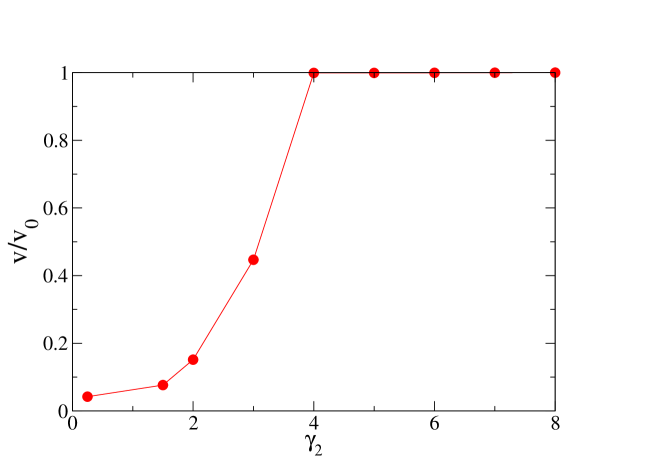
Figure 6: (color online): Plot of normalised velocity difference $\Delta v/v_{0}$ vs. $\gamma_{2}$ for ordered state when $\eta=0.2$.

III.4 Disordered phase segregated: DPS

Now we tune noise to larger values $\eta>0.6$ and vary the variable speed parameter $\gamma_{2}$. For large $\gamma_{2}>3$, i.e. for type one $\gamma_{1}=1$ particle speed vary linearly with local polarisation and for second type $\gamma_{2}>>\gamma_{1}$, speed is close to maximum speed for well ordered regions and very small for disordered region. In the disordered region when $\eta>0.6$, most of the time particles are in disordered cluster region or moving individually. For type one particle since speed vary linearly with local polarisation hence we find a broad distribution of $P(v)$ and another type particle, speed can mainly take two possible values $0$ and $v_{0}$ when particle moves individually or in cluster respectively. In Fig. 1(e) and (e’) we plot the real space snapshot of particle position for both types of particles. We find that one type of particles, for which $\gamma$ is large forms more or less static clusters shown in red and other type of particles are part of the static cluster partially and partially they are moving randomly (as shown in black arrow in Fig. 1(e)) . In the bottom panel we show the zoomed version of the same snapshot for small part of the total system. Which shows that orientation of particles inside the cluster is random. In Fig. 4 we plot $P(v)$, which shows a broad distribution for type one particles and two distinct peaks at $v=0.5$ and $v=0.0$ for type two particles. Which again due to static clusters. Size of the peak at $v=0.5$ is large for type one particle in comparison to second type. Hence large number of type one particles are moving randomly. To further characterise this phase also plot the four $P_{ij}(n)$’s. In this case the four distribution are very different from the previous cases. We find that $P_{11}(n)$ is Gaussian and shows a peak at some finite value of $n$. That typically represent the mean number of particles in the interaction radius. This is due to presence of type one particle in the static regions of cluster formed by second type particles, which acts like nucleation site for particle of type one. The $P_{12}(n)$, shows a broad distribution which confirms that the cluster of particle of type one has another particle too (due to fixed second type particle). The two other distributions $P_{22}(n)$ and $P_{21}(n)$ are similar. When plotted on log-log scale, the two $P_{21}$ and $P_{22}$ shows exponential tail with $n_{0}\approx 5$

III.5 Dynamics of particle in DM and DPS phase

We also characterise the dynamics of both types of particles in DM and DPS phase. We first calculate the mean square displacement MSD $\Delta_{i}(t)=<|{\bf r}_{i}(t+t_{0})-{\bf r}_{i}(t)|^{2}>$, where $i=1,2$ for particle of type one and two respectively. $<.>$ is over all the particles of same type and many reference time $t_{0}$. MSD is calculated for $\eta=0.62$ and for different $\gamma_{2}$. In the disordered region or when $\eta>0.6$ we find that for both $\Delta_{i}(t)\simeq t$, which suggest the diffusive behavior of particles. We further estimate the effective diffusion coefficient $D_{eff}=\lim_{t\rightarrow\infty}\frac{\Delta(t)}{4t}$. Hence in Fig. 7 we plot the effective diffusion coefficient $D_{eff}$ vs. $\gamma_{2}$. For small $\gamma_{2}$ diffusivity of both types particle is finite but as we increase $\gamma_{2}$, diffusivity of second type particle is almost zero. Which suggest static clusters of second type particle as found in DPS phase.

6

Figure 7: Plot of effective diffusivity $D_{eff}$ vs. $\gamma_{2}$ in the disordered region $\eta=0.65$ for two types of particles. $\circ$, $\square$ is for particle of type one and two respectively. Other parameters are same as given in Fig. 1

IV Discussion

We have studied the binary mixture of polar self-propelled particles with variable speed. Speed of the particle depends on its neighbors and its maximum in well aligned region and almost zero in random disorder region. Dependence of local speed on local orientation is controlled by a variable speed parameter $\gamma$. The model is motivated with experiments on fish school where speed of individual fish depends on their neighbors. We mix the two different types of particles with two different $\gamma$ values. One of the $\gamma_{1}$ is fixed to $1$ and another $\gamma_{2}$ is varied from $0$ to $8$. For $\gamma=0$ model reduces to constant speed model. Steady state behavior of the system is studied for different combination of $(\gamma_{2},\eta)$. For all set of $\gamma$’s system shows a transition from disordered state to ordered state. We find four different phases: (i) ordered phase separated (OPS) when noise is small and difference in two $\gamma$’s is large. In this phase starting from random mixed phase both types of particle phase separate and moves in different clusters. (ii) ordered mixed phase (OM), when the difference is $\gamma$ is small then all the particles moves in well ordered cluster but in a single cluster both types of particles are present, (iii) disorder mixed phase (DMP), when $\eta$ is large and different in two $\gamma$ is small then both orientation and density order parameter is small and both types of particles remain is mixed phase and have random orientation. (iv) disorder phase segregated (DPS), when one of the $\gamma$ is large and noise in also large then local orientation is small hence for larger $\gamma_{2}$, speed of the second type of particle is almost zero and hence they form static clusters and speed of the first types particle varies linearly with local polarisation. Second type of particle which form static cluster with completely random orientation acts like nucleation site and then first type of particle come in contact with the static cluster they also form small clusters there. Which leads to a characteristic cluster size for first type particle. Hence our study shows appearance of different phases in binary active mixture of SPP’s with variable speed. The variable speed parameter introduced here can be thought of as characteristic of particle. Hence our study give insight to phase separation in different particle types. Also it opens new direction to study these systems in detail. It is also interesting to study the ordering kinetics ajbray of two types particle in such mixture.

V Mean-field order-disorder transition using coarse-grained hydrodynamics

We begin by defining the coarse-grained local density field for two types of particles. For particle of type one

$$\rho_{1}({\bf r},t)=\sum_{i=1}^{N_{1}}\delta({\bf r}-{\bf r}_{i})$$ (5)

and for type two

$$\rho_{2}({\bf r},t)=\sum_{j=1}^{N_{2}}\delta({\bf r}-{\bf r}_{j})$$ (6)

where ${\bf r}_{i}$ and ${\bf r}_{j}$ is position vector of particle of type one and two. Similarly we define the local coarse-grained polarization field as

$${\bf P}({\bf r},t)={\frac{{\sum}^{N}_{k=1}\bf n_{i}(t)\delta(\bf r-r_{k})}{\rho({\bf r},t)}},$$ (7)

where $N=N_{1}+N_{2}$ and $\rho=\rho_{1}+\rho_{2}$ and $\sum_{k}$ is over all the particles. Using the update rules of position Eq. 1, orientation Eq. 2 and using the same analysis as in shradhanjop ; shradhathesis ; shradhapre2012 ; shradhamanna , we now write the stochastic partial differential equations of motion for two coarse-grained densities $\rho_{1}({\bf r},t)$ and $\rho_{1}({\bf r},t)$ and polarisation vector $P({\bf r},t)$ as defined in Eqs. 5, 6, 7. We begin with density equation for type one particle.

$$\rho_{1}({\bf r},t+\Delta{t})-\rho_{1}({\bf r},t))={\sum}^{N_{1}}_{i=1}[\delta({\bf r}-{\bf r}_{i}(t+\Delta{t})]-\delta[{\bf r}-{\bf r}_{i}(t)]$$

$$\Rightarrow-{\sum}^{N_{1}}_{i=1}v_{i}(t)\bf n_{i}(t)\nabla\delta[{\bf r}-{\bf r}_{i}(t)]+\frac{1}{2}{\sum}^{N_{1}}_{i=1}{\sum}^{N_{1}}_{i^{\prime}=1}v^{2}_{i}{\bf n_{i}}(t){\bf n_{i^{\prime}}}(t):\nabla_{i}\nabla_{i}^{\prime}\delta[{\bf r}-{\bf r_{i}}(t)]$$ (8)

Now we substitute for variable speed from Eqs. 3 and 4 and dividing by $\Delta{t}$ and taking the limit $\Delta{t}\longrightarrow{0}$

$$\partial_{t}\rho_{1}({\bf r},t) =v_{0}{\sum}^{N_{1}}_{i=1}[{[\frac{{\sum}^{R_{0}}_{j}{\bf n}_{j}}{N_{i}}]}^{\gamma_{1}}v_{i}(t){\bf n}_{i}(t)\nabla\delta[{\bf r}-{\bf r}_{i}(t)] +v_{0}^{2}\frac{1}{2}{\sum}^{N_{1}}_{i=1}{\sum}^{N_{1}}_{i^{\prime}=1}[\frac{{\sum}^{R_{0}}_{j}{\sum}^{R_{0}}_{j^{\prime}}{\bf n}_{j}{\bf n}_{j}^{\prime}}{N_{i}N_{i}^{\prime}}]^{\gamma_{1}}:\nabla_{i}\nabla_{i}^{\prime}\delta[{\bf r}-{\bf r}_{i}(t)]$$

Here the operator “$:$” is the double dot (or colon) product defined by ${\bf ab:cd}=\sum_{\alpha}\sum_{\beta}{a^{\alpha}b^{\beta}c^{\alpha}d^{\beta}}$, with indexes $\alpha$ and $\beta$ indicating the vector components $(1,2)$. The expansion in equation Eq. 8 and V is valid for small values of the order parameter field and small particle speed, such that the displacement per time step is much smaller than the interaction range. We now use mean-field approximation and replace the summation over particle inside the interaction radius $R_{0}$ by mean value of polarisation we find the final equation for the density field $\rho_{1}$ as

$${\partial_{t}\rho_{1}}=-\nabla\cdot(v_{1}{\bf P}\rho_{1})+D{\nabla}^{2}(v_{1}^{2}\rho_{1})$$ (9)

where $v_{1}$ is self-propulsion speed of particle and in general depends on local polarisation. In the same manner we can also derive the density equation for second type particle

$${\partial_{t}\rho_{2}}=-\nabla\cdot(v_{2}{\bf P}\rho_{2})+D{\nabla}^{2}(v_{2}^{2}\rho_{2})$$ (10)

Where $D$ is introduced as diffusion coefficient, which is function of microscopic parameters. Here we assume it to be constant. Now we come to the equation for the polarisation order parameter. After a long but straight-forward calculation as in shradhanjop ; shradhathesis ; shradhapre2012 ; shradhamanna ; tonertu and in the mean-field limit as for density equations 9 and 10, the polarisation equation will have mainly following terms

$$\partial_{t}{\bf P}=(\alpha_{1}(\rho,\eta)-\alpha_{2}{\bf P}\cdot{\bf P}){{\bf P}}-\frac{v_{1}}{2}\nabla\rho_{1}-\frac{v_{2}}{2}\nabla\rho_{2}+\lambda({\bf P}\cdot\nabla){\bf P}+k\nabla^{2}{\bf P}+{\bf H}$$ (11)

where on the R. H. S. of above equation the first term is the polynomial term which determines the order-disorder mean field transition. The second and third terms, the two gradients in density, is the change in local polarisation due to the variation in density of two types of particles, $\lambda$ term in the non-linear term and coefficient $\lambda$ in general depends on the microscopic parameters viz (mean density $\rho_{0}$, speed ${\bf v_{0}}$ etc.). In general we have three kinds of non-linearities as given in shradhanjop ; shradhathesis ; shradhapre2012 ; shradhamanna ; tonertu but we keep only one of the relevant one as shown in recent study of tonertupre2018 . The last term is the diffusion of local polarisation and $\bf H$ is the stochastic noise term with $H=\sqrt{\rho}{\bf M\bf h}$ Here $\bf h(r,t)$ is a vector field of unit length and random orientation, delta correlated in space and time, while $\bf M(r,t)$ is a $2\times{2}$ tensor field satisfying $\bf M^{2}=1$. Here we are mainly interested in the mean-field order-disorder transition which is mainly predicted by $\alpha_{1}(\rho,\eta)$.When derived from microscopic and and in the mean-field limit $\alpha_{1}(\rho,\eta)=(\rho_{0}-4\eta^{2})$. Hence we find that $\alpha_{1}$ is only function of mean density $\rho_{0}$ and noise $\eta$ and is independent of the variable speed parameter $\gamma$. Which confirms the disorder-to-order transition remains invariant with respect to the $\gamma$ as found in our numerical simulation.

VI Linearised study of hydrodynamic equations of motion

In this section we will do the linearised study of hydrodynamic equations of motion derived for the two density fields and polarisation Eqs. 9, 10 and 11. We take the mean-field approximation so that the speed of two particles can be replaced by $v_{1,2}=v_{0}(p_{0})^{\gamma_{1},\gamma_{2}}$, where $p_{0}=\sqrt{\frac{\alpha_{1}}{\alpha_{2}}}$ in Eq. 11. Using the two density equation we write the equation in terms of difference in the density of both types of particle $\Delta\rho=\rho_{1}-\rho_{2}$

$$\partial_{t}\Delta\rho=-v_{1}\nabla\cdot({\bf P}\rho_{1})+v_{2}\nabla\cdot({\bf P}\rho_{2})+D\nabla^{2}\Delta\rho$$ (12)

which is further equal to

$$\partial_{t}\bigtriangleup\rho=-\bigtriangleup{v}\nabla\cdot({\bf P}\rho_{1})-v_{2}\nabla\cdot({\bf P}\bigtriangleup\rho)+D\nabla^{2}\bigtriangleup\rho$$ (13)

where $\Delta v=v_{1}-v_{2}$. and equations for the density of particle of type one is same as in Eq. 10. In the same manner we write the polarisation equation also in terms of $\Delta\rho$ and $\Delta v$

$$\partial_{t}{\bf P}=(\alpha_{1}(\rho,\eta)-\alpha_{2}{\bf P}\cdot{\bf P}){{\bf P}}-\frac{\overline{v}}{2}\nabla(v_{1}\rho_{1})+\frac{v_{1}}{2}\nabla(\Delta\rho)-\frac{\Delta v}{2}\nabla(\Delta\rho)+\lambda({\bf P}\cdot\nabla){\bf P}+k\nabla^{2}{\bf P}+{\bf H}$$ (14)

The homogeneous steady state solution of above three equations for $\Delta\rho$, $\rho_{1}$ and ${\bf P}$ is $\Delta\rho=0$, $\rho_{1}=0$ and ${\bf P}=\sqrt{\frac{\alpha_{1}}{\alpha_{2}}}{\widehat{\bf x}}$ (the direction of broken symmetry along $x-$axis). We add small perturbation about the above homogeneous solution hence $\Delta\rho_{1}=\delta\Delta\rho$, $\rho_{1}=\rho_{10}+\delta\rho_{1}$ and ${{\bf P}}=(p_{0}+\delta{p_{\parallel}}){\widehat{\bf x}}+(\delta{p}_{\perp}){\widehat{\bf y}}$, where $p_{0}=\sqrt{\frac{\alpha_{1}}{\alpha_{2}}}$ and $\delta\Delta\rho=\delta\rho_{1}-\delta\rho_{2}$ is the fluctuation is the two densities about their mean values. Now we write the equations for small perturbations in four fields $\Delta\rho$, $\delta\rho_{1}$, $\delta p_{\parallel}$ and $\delta p_{\perp}$. We first write the equation for $p_{\parallel}$ first

$$\partial_{t}\delta{p}_{\parallel}=(\alpha_{1}(\rho_{0})-\alpha_{2}(p_{0}^{2}+2p_{0}\delta{p}_{\parallel}))(p_{0}+\delta{p}_{\parallel})-\frac{v_{1}}{2}\nabla\delta\rho_{1}-\frac{v_{2}}{2}\nabla(\rho_{1}-\bigtriangleup\rho)+\lambda(p_{0}\delta_{x})\delta{p}_{\parallel}+k\nabla^{2}\delta{p}_{\parallel}$$ (15)

If we ignore the higher order gradients terms we find in the steady state

$$\delta{p}_{\parallel}=-\frac{v_{1}}{4\alpha_{1}}(v_{1}+v_{2})\nabla_{x}\delta\rho_{1}+\frac{v_{2}}{4\alpha_{1}}\nabla_{x}(\bigtriangleup\rho)\\$$ (16)

Now we write the equations for the small fluctuations in other three field and substitute the expression for $\delta P_{\parallel}$ from Eq. 15

$$\partial_{t}\delta{p}_{\perp}=-\frac{v_{1}}{2}\delta_{y}\delta\rho_{1}-\frac{v_{2}}{2}\delta_{y}(\delta\rho_{1}-\bigtriangleup\rho)+\lambda(p_{0}\delta_{x})\delta{p}_{\perp}+k\nabla^{2}\delta{p}_{\perp}$$ (17)

substitute from Eqs. V, 9 and 12, from equation 16, we solve for $\partial{p}_{\parallel}$ and substitute in equation 17

$$\partial_{t}\delta{p}_{\perp}=-v_{1}p_{0}\delta_{x}\delta\rho_{1}+\frac{v_{1}\rho_{10}}{4\alpha_{1}}\overline{v}\delta_{x}^{2}\delta\rho_{1}-\frac{v_{1}v_{2}\rho_{1}0}{4\alpha_{1}}\delta_{x}^{2}\bigtriangleup\rho-v_{1}\rho_{10}\delta_{y}\delta{p}_{\perp}+D\nabla^{2}\delta\rho_{1}\\$$ (18)

where $\overline{v}=v_{1}+v_{2}$, similarly we write equations for $\partial_{t}\delta\rho_{1}$ and $\partial_{t}\Delta\rho$

$$\partial_{t}\delta\rho_{1}=-v_{1}\delta_{x}((p_{0}+\delta{p}_{\parallel})(\rho_{10}+\delta\rho_{1}))-v_{1}\delta_{y}(\delta{p}_{\perp}\rho_{10})+D\nabla^{2}\delta\rho_{1}\\$$ (19)

$$\partial_{t}\bigtriangleup\rho=-\bigtriangleup{p_{0}}\delta_{x}\delta\rho_{1}+\frac{\bigtriangleup\overline{v}\rho_{10}\delta_{x}^{2}\delta\rho_{1}\overline{v}}{4\alpha_{1}}-\frac{\bigtriangleup{v}\rho_{10}v_{2}\delta_{x}^{2}\bigtriangleup\rho}{4\alpha_{1}}-\bigtriangleup\rho_{10}\delta_{y}\delta{p}_{\perp}-v_{2}p_{0}\delta_{x}\bigtriangleup\rho+D\nabla\bigtriangleup\rho\\$$ (20)

now taking the Fourier transformation equation 17 18 and 19 by using

$$Y=\begin{bmatrix}\partial\rho_{1}\\ \partial{p_{\perp}}\\ \Delta\rho\end{bmatrix},Y(k,S)=\int{Y(r,t)}\exp{(S{t}-i\overline{k}\cdot\overline{r})}d\overline{r}dt$$ (21)

and write in Fourier space

$$(S+v_{1}+p_{0}iq_{x}+\frac{v_{1}\rho_{10}\overline{v}q_{x}^{2}}{4\alpha_{1}}+Dq^{2})\delta\rho_{1}-(\frac{v_{1}v_{2}\rho_{10}q_{x}^{2}}{4\alpha_{1}})\bigtriangleup\rho+v_{1}\rho_{10}iq_{y}\delta{p}_{\perp}=0\\$$ (22)

$$(\bigtriangleup{v}p_{0}iq_{x}+\frac{\bigtriangleup{v}\overline{v}\rho_{10}q_{x}^{2}}{4\alpha_{1}})\delta\rho_{1}+(S-\frac{\bigtriangleup{v}v_{2}\rho_{10}q_{x}^{2}}{4\alpha}+Dq^{2}+v_{2}p_{0}iq_{x})\bigtriangleup\rho+\bigtriangleup{v}\rho_{10}iq_{y}\delta{p}_{\perp}=0\\$$ (23)

$$(\frac{v_{1}iq_{y}}{2}+\frac{v_{2}iq_{y}}{2})\delta\rho_{1}-(\frac{v_{2}iq_{x}}{2})\bigtriangleup\rho+(S-\lambda{p_{0}}iq_{x}+kq^{2})\bigtriangleup{p}_{\perp}=0\\$$ (24)

$M\times{Y}=0$ where

$$M=\begin{bmatrix}(S+v_{1}p_{0}iq_{x}+\frac{v_{1}\rho{10}\overline{v}q_{x}^{2}}{4\alpha_{1}}+Dq^{2})&(-v_{1}v_{2}\rho_{10}q_{x}^{2}/4\alpha_{1})&(v_{1}\rho_{10}iq_{y})\\ (\bigtriangleup{v}p_{0}iq_{x}+\frac{\bigtriangleup\overline{v}\rho_{10}q_{x}^{2}}{4\alpha_{1}})&(S-\frac{\bigtriangleup{v}v_{2}\rho{10}q_{x}^{2}}{4\alpha_{1}}+Dq^{2}+v_{2}p_{0}iq_{x})&(\bigtriangleup\rho_{10}iq_{y})\\ (\frac{\overline{v}}{2}iq_{y})&(-\frac{v_{2}}{2}iq_{y})&(S-\lambda{p_{0}iq_{x}}+kq^{2})\end{bmatrix}\begin{bmatrix}\delta\rho_{1}\\ \delta{p}_{\perp}\\ \bigtriangleup\rho\end{bmatrix}$$ (25)

Now we focus along the ordering direction $q_{y}=0,\theta=0,q_{x}=q$ and $det[M]=0$
Eq 25 can be solved for modes by det$[M]=0$

$$0=\begin{bmatrix}(S+v_{1}p_{0}iq+\frac{v_{1}\rho{10}\overline{v}q^{2}}{4\alpha_{1}}+Dq^{2})&(-v_{1}v_{2}\rho_{10}q^{2}/4\alpha_{1})&0\\ (\bigtriangleup{v}p_{0}iq+\frac{\bigtriangleup\overline{v}\rho_{10}q^{2}}{4\alpha_{1}})&(S-\frac{\bigtriangleup{v}v_{2}\rho{10}q^{2}}{4\alpha_{1}}+Dq^{2}+v_{2}p_{0}iq)&0\\ 0&0&(S-\lambda{p_{0}iq}+kq^{2})\end{bmatrix}$$ (26)

One of the mode $\Rightarrow{S=\lambda{p}_{0}iq-kq^{2}}$ Damped-diffusive oscillatory modes and other two modes are given by

$$0=\begin{bmatrix}(S+v_{1}p_{0}iq+q^{2}(D+\frac{v_{1}\rho_{10}\overline{v}}{4\alpha_{1}})&(-v_{1}v_{2}\rho_{10}q^{2}/4\alpha_{1})\\ (\bigtriangleup{v}p_{0}iq+\frac{\bigtriangleup{v}\overline{v}\rho_{10}q^{2}}{4\alpha_{1}})&(S+v_{2}p_{0}iq+q^{2}(D-\frac{v_{2}\rho_{10}\bigtriangleup{v}}{4\alpha_{1}})\end{bmatrix}$$ (27)

lets define $D_{+}=q^{2}(D+\frac{v_{1}\rho_{10}\overline{v}}{4\alpha_{1}})$ and $D_{-}=q^{2}(D-\frac{v_{2}\rho_{10}\bigtriangleup{v}}{4\alpha_{1}})$ Hence we have two solutions for $S$, $\mathcal{R}e(S)>0$ (mode is unstable) and when $\mathcal{R}e(S)<0$ (then it is stable)

$$(S+v_{1}p_{0}iq+q^{2}D_{+})(S+v_{2}p_{0}iq+q^{2}D_{-})+\frac{v_{1}v_{2}\rho_{10}\bigtriangleup{v}p_{0}iq^{3}}{4\alpha_{1}}+\frac{\bigtriangleup{v}\overline{v}v_{1}v_{2}\rho_{10}^{2}q^{4}}{(4\alpha_{1})^{2}}=0\\$$ (28)

$${2S}_{\pm}=[(v_{1}p_{0}iq+D_{+q}^{2})+(v_{2}p_{0}iq+D_{-}q^{2})]\pm[(v_{1}p_{0}iq+D_{+}q^{2})-(v_{2}p_{0}iq+D_{-}q^{2})]$$ (29)

$${S}_{+}=[(v_{1}p_{0}iq+D_{+q}^{2})+(v_{2}p_{0}iq+D_{-}q^{2})]+[(v_{1}p_{0}iq+D_{+}q^{2})-(v_{2}p_{0}iq+D_{-}q^{2})]$$ (30)

The $-Ve$ root $S_{-}=-2(v_{1}p_{0}iq+D_{+}q^{2})\rightarrow$, is always stable The $+Ve$ root $S_{+}$ can become unstable since $p_{0}<1$ as if $\bigtriangleup{v>\frac{4D\alpha_{1}}{v_{2}\rho_{10}}}\Rightarrow(\frac{\textbullet 8D\alpha_{1}}{v_{2}\rho_{0}})$. Hence criticality arise at $\bigtriangleup{v}=\frac{8D\alpha_{1}}{\rho_{0}v_{0}p_{0}^{\gamma_{2}}}$ As $\gamma_{2}$ increases the difference in two speeds $\Delta v$ also increases which leads to more instability. Similar trend is obtained in our numerical simulation when difference in two $\gamma{{}^{\prime}s}$ large than order-homogeneous state is unstable.

References

- (1) T. Feder, Phys. Today 60(10), 28 (2007); C. Feare, The Starling (Oxford University Press, Oxford, 1984).
- (2) E. Rauch, M. Millonas, and D. Chialvo, Phys. Lett. A 207, 185 (1995).
- (3) Toner J, Tu Y, and Ramaswamy S 2005 Ann. Phys. (Amsterdam) 318 170.
- (4) Ramaswamy S 2010 Annu. Rev. Condens. Matter Phys. 1 323.
- (5) Marchetti M C et al. 2013 Rev. Mod. Phys. 85 1143.
- (6) Harada, Y., Nogushi, A., Kishino, A. and Yanagida, T. Nature (London) 326, 805–808 (1987).
- (7) Badoual, M., Jülicher, F. and Prost, J. Proc. Natl. Acad. Sci. U.S.A. 99, 6696–6701 (2002).
- (8) Nédélec, F. J., Surrey, T., Maggs, A. C. and Leibler, S. Nature (London) 389, 305–308 (1997).
- (9) Rauch, E. M., Millonas, M. M. and Chialvo, D. R. Phys. Lett. A 207, 185–193 (1995).
- (10) Ben-Jacob, E. et al. Phys. Rev. Lett. 75, 2899–2902 (1995).
- (11) Appleby, M. C. (ed. Parrish, J. K. and Hamner, W. M.) (Cambridge: Cambridge University Press, 1997).
- (12) Helbing, D., Farkas, I. and Vicsek, T. Nature 407, 487–490 (2000).
- (13) Helbing, D., Farkas, I. J. and Vicsek, T. Phys. Rev. Lett. 84, 1240–1243 (2000).
- (14) Kuusela, E., Lahtinen, J. M. and Ala-Nissila, T. Phys. Rev. Lett. 90, 094502 (2003).
- (15) Hubbard, S., Babak, P., Sigurdsson, S. and Magnusson, K. Ecological Modeling 174, 359–374 (2004).
- (16) Schaller, V., Weber, C., Semmrich, C., Frey, E. and Bausch, A. R. Nature 467, 73–77 (2010).
- (17) Sumino, Y. et al. Nature 483, 448–452 (2012).
- (18) Peruani, F. et al. Collective motion and nonequilibrium cluster formation in colonies of gliding bacteria. Phys. Rev. Lett. 108, 098102, 2012.
- (19) Ben-Jacob E, Cohen I, Shochet O, Czirk A and Vicsek T 1995 Phys. Rev. Lett. 75 2899 (1995).
- (20) Vicsek T et al. 1995 Phys. Rev. Lett. 75 1226 (1995).
- (21) Chat H, Ginelli F, Grgoire G and Raynaud F 2008 Phys. Rev. E 77 046113.
- (22) Chat H, Ginelli F and Grgoire G 2007 Phys. Rev. Lett. 99 229601.
- (23) Y. Katz, K. Tunstrøm, C. C. Ioannou, C. Huepe, and I. D. Couzin, Proc. Natl. Acad. Sci. USA 46, 18720 (2011).
- (24) S Pattanayak, S Mishra Journal of Physics Communications 2 (4), 045007, (2018).
- (25) B Bhattacherjee, S Mishra, SS Manna Phys. Rev.E 92 (6), 062134, (2015).
- (26) Luis H. Cisneros, John O. Kessler, Sujoy Ganguly, and Raymond E. Goldstein Phys. Rev. E 83, 061907, (2011).
- (27) S Mishra, K Tunstrøm, ID Couzin, C Huepe Phys. Rev. E 86 (1), 011901, (2012).
- (28) A. J. Bray, Adv. Phys. 43, 357 (1994).
- (29) E Bertin, H Chaté, F Ginelli, S Mishra, A Peshkov, S Ramaswamy New J. of phys. 15 (8), 085032, (2013).
- (30) S. Mishra, Ph.D. thesis, Indian Institute of Science, Bangalore, 2009, [http://www.openthesis.org/document/view/601122/0.pdf].
- (31) Toner J and Tu Y Phys. Rev. Lett. 75 4326 (1995); Phys. Rev. E 58 4828, (1998).
- (32) J. Toner, N. Guttenberg, and Y. Tu, Phys. Rev. E 98, 062604 (2018).