Causal Simulations for Uplift Modeling

Abstract

Uplift modeling requires experimental data, preferably collected in random fashion. This places a logistical and financial burden upon any organisation aspiring such models. Once deployed, uplift models are subject to effects from concept drift. Hence, methods are being developed that are able to learn from newly gained experience, as well as handle drifting environments. As these new methods attempt to eliminate the need for experimental data, another approach to test such methods must be formulated. Therefore, we propose a method to simulate environments that offer causal relationships in their parameters.

Introduction

In uplift modeling, the effect $E$ of a cause $C$ applied on an entity $\mathbf{x}$ is estimated. Effect is defined as a measure of behaviour. When this behaviour is paired with a higher probability of occurring after the application of $C$, an uplift is associated. In essence, the uplift is thus the positive net impact of $C$ on $E$ for a specific $\mathbf{x}$, as defined in (1).

$$U(C,E,\mathbf{x})\doteq p(E=1|C=1,\mathbf{x})-p(E=1|C=0,\mathbf{x})$$ (1)

While above formulation describes the objective, it is impossible to derive from data due to the fundamental problem of causal inference (?). As such, an estimation of the uplift $\hat{u}(C,E,\bm{\phi}(\mathbf{x}))$ over a generalisation $\bm{\phi}(\cdot)$ of the entities is needed. Typical applications of such models are found in direct marketing (?), as well as medical scenarios (?).

While the collection of experimental data in the context of direct marketing seems acceptable, the inability to handle concept drift is not (?; ?). Contrasting a medical setting where concept drift is likely of lesser concern. However, the randomised collection of experimental data could prove problematic. This due to the need for a sufficient amount of controlled – or untreated – cases.

Alas, every model is learned on the basis of data. However, the method of gathering this data tends to quickly diverge from a purely random manner, given an experienced based learner as defined in the field of reinforcement learning (RL).

While in RL some state could potentially transition to a subsequent state, in this first formalisation this consideration is omitted in favour of bandit algorithms (?). Research on causally aware bandits is reliant on either a real environment (?; ?), or a simulation (?; ?; ?; ?). Depending on the projected use of the model, testing experimental algorithms on a real environment might prove detrimental.

It is therefore crucial to formulate a variety of simulated environments to both validate and benchmark these algorithms. As such, a simulation offers the ability to consult a ground truth – or counterfactual – to properly measure performance. This research contributes a method by which such causal simulations are to be created. The method presented is highly generic and covers a wide range of situations a causal bandit could be faced with.

Simulating an environment

When constrained with $C\in\{0,1\}$, an uplift model provides an estimated difference between two conditional probabilities. If such a difference is absent, $C$ does not offer any causal relationships in the environment. Therefore, this difference is assumed. As such, any causal simulation should provide at least two distinct distributions; $\mathcal{D}_{0}$ for the controlled cases, and $\mathcal{D}_{1}$ for the treated cases where $E\sim\mathcal{D}_{i}=p(E=1|C=i,\mathbf{x})\in\mathbb{D}$ as in (1).

When $k$ causes are to be modeled, the simulation ought to provide $k+1$ distributions. A difference could be caused by the interaction of unobserved confounders (?). Any unobserved confounder will introduce a dimension to $\mathcal{D}_{i}$ and is discussed in a following section.

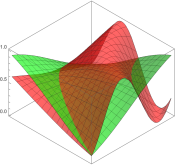
(a) Sine base, with $\lambda(C=0)=2$, $\lambda(C=1)=1$ and $\mathbf{g}=(0.7,0.7)^{T}$

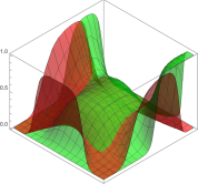
(b) Polynomial base, with $q=5$

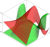
(c) Mixture base

Figure 1: Examples of different $b$ in two dimensions where green is $p_{\text{sim}}(E=1|C=1,\mathbf{x})$ and red is $p_{\text{sim}}(E=1|C=0,\mathbf{x})$

Requirements of a simulation

A number of elements are required in order to simulate a real environment. These elements should be taken into account by the signature of a simulation and are defined as follows.

Drift

In order to test algorithms against drift, in function of time, drift must be made a parameter. This can be modeled numerically as $d(t):t\rightarrow\mathbb{R}^{+}$, exerting an influence on a simulation while remaining unknown to the algorithms. If $d(t)$ fluctuates heavily, a more volatile simulation is created. Less so when $d(t)$ remains stagnant.

Base functions

Given a single cause situation ($C\in\{0,1\}$), while considering a binary effect ($E\in\{0,1\}$), four different combinations of $C$ and $E$ can be formulated. As such, a simulation should account for these combinations through the aforementioned two distributions $\mathcal{D}_{i}$. In their most extreme case, the probabilities associated with $p(E=1|C,\mathbf{x})$ are $0$ and $1$ and must be paired with both states of $C$. Any interpolation between these probabilities is left to the functional form of the distribution. The complexity of this interpolation will impose a degree of difficulty for the tested algorithm and its method of approximation and should thus be parametrised through what we define as a base function $b$,

$$b(C,\mathbf{x},d(t)):C\times\mathbf{x}\times d(t)\rightarrow[0,1],$$ (2)

$\mathbb{D}$ can now be simulated by $b$ where $\mathcal{D}_{i}$ is simulated by $b(C=i,\mathbf{x},d(t))$ which we shall denote $b_{i}$.

Effect

An algorithm capable of handling the environment directly, must operate while only receiving some $\mathbf{x}$ and $E$ after the application of their chosen $C$. In this binary effect situation, the simulation should return either $1$ or $0$ representing $E$, as in reality. As such, any value from $b$ will be used as a parameter in a Bernoulli experiment.

Evaluation

The target of an optimal uplift model is to only apply $C$, when $\mathbf{x}$ presents a positive causal relationship to $E$. The notion of this relationship can be presented to the evaluation method as the ground truth is now known through $b_{i}$. Furthermore, different intrecacies of the simulation might form additional interest as the evaluation method is highly dependent on the target an algorithm optimises for. With $b_{i}$, such intrecacies can be shared to other evaluation methods.

Composing the simulation

We now turn to the problem of composing different $b_{i}$. Depending on the dimensions describing $\mathbf{x}\in\mathbb{R}^{N}$, the domain $\mathbf{d}\in\mathbb{R}^{M}$ of $b$ holds different implications.

When $N>M$, some dimensions of $\mathbf{x}$ will have no influence on $\mathcal{D}$, rendering them obsolete. With $N=M$, every dimension will influence $\mathcal{D}$. In the case of $N<M$, a group of size $M-N$ unobserved confounders are simulated. To account for an $M$-dimensional domain, a base function $b$ must be called with some $\mathbf{x^{\prime}}=(\mathbf{x},\mathbf{u})^{T}$, where $\mathbf{u}\in\mathbb{R}^{M-N}$ represents the unobserved confounders. The larger the influence of $\mathbf{u}$ on $b$ and thus $\mathcal{D}$, the stronger the influence of the confounder. As the name indicates, $\mathbf{u}$ ought to remain unobservable, i.e. remain unknown, to the tested algorithm.

The manner in which the dimensions of $\mathbf{x^{\prime}}$ interactively influence the simulation is left to $b$. As such, the method by which $\mathbf{u}$ confounds $\mathcal{D}$ is another parameter of difficulty for the algorithm, though one which we will not further explore in this first formalisation.

While many implementations can be defined for $b$, we present three different approaches, each with its own advantages and disadvantages.

Sine base

One approach is to make use of the trigonometric functions (Figure 1(a)). This due to their periodic nature, useful for $d(t)$. Their output range $[-1,1]$ is linearly adjusted in (3), with $\mathbb{I}(\cdot)$ as the indicator function and $b(C,\mathbf{x^{\prime}},d(t))$ denoted $b$ for brevity,

$$b_{i}=\frac{1}{2}\left[\sin\left(d(t)+\lambda_{i}\prod^{M}\left[\mathbf{x^{\prime}}_{m}+\mathbb{I}(i=0)\mathbf{g}_{m}\right]\right)+1\right],$$ (3)

while drift $d(t)$ is accounted for through simple summation, interaction in the dimensions of $\mathbf{x^{\prime}}$ is achieved by multiplication. The complexity of $b_{i}$ is parametrised through the addition of a positive integer $\lambda_{i}$, governing the frequency of its sine wave such that every cause ($C=i$) could have a different complexity. A displacement vector $\mathbf{g}\in\mathbb{R}^{M}$, monitors the strength of the causal relationship as $\mathbf{g}$ will provide a difference between $\mathcal{D}_{i}$. If $\mathbf{g}=\mathbf{0}$ no difference is accounted for. A disadvantage of such sine base is the relative ease in which their shapes are estimated.

Polynomial base

An alternative to the sine base is the polynomial base in (4). Where $\sigma(\cdot)$ is the logistic sigmoid function, binding the polynomial to a range of $[0,1]$. The polynomial base offers more erratic shapes than the sine base (Figure 1(b)), allowing for more rigorous testing. As such, testing using this polynomial base will be more involved with regards to the approximation method.

$$b_{i}=\sigma\left(\left(\mathbf{k}_{i}+h(d(t))\mathbf{1}\right)^{T}\bm{\upsilon}_{i}(\mathbf{x^{\prime}})\right)$$ (4)

With coefficients $\mathbf{k}_{i}\in\mathbb{R}^{q}$, where $\mathbf{k}_{0}\neq\mathbf{k}_{1}$ and $q\in\mathbb{N}^{+}$, $h(d(t))\rightarrow[a,b]$ ensuring some periodic evolution in the interval $[a,b]$, $\mathbf{1}$ as a $q$-dimensional vector with $\mathbf{1}_{j}=1\text{ }\forall\text{ }j=1,2,...,q$ and

$$\bm{\upsilon}_{i}(\mathbf{x^{\prime}})\doteq\left(1,\prod^{1}\upsilon(\mathbf{x^{\prime}}),\prod^{2}\upsilon(\mathbf{x^{\prime}}),...,\prod^{q-1}\upsilon(\mathbf{x^{\prime}})\right)^{T},$$

where $\bm{\upsilon}_{0}(\mathbf{x^{\prime}})\neq\bm{\upsilon}_{1}(\mathbf{x^{\prime}})$ and $\upsilon(\cdot)$ will uniformly select one dimension of $\mathbf{x^{\prime}}$ providing a polynomial interaction with a maximum degree of $q-1$, leaving $q$ to be a parameter of complexity.

Prior model base

An argument against above base functions is one of reality. These base functions offer a wide range of complexity, both in approximation and in causality, yet their complexity comes entirely from a numerical perspective. A more reality based $b$ could be a previously trained model, which despite lacking a method to incorporate $d(t)$ as in (2), could prove useful to relieve a new model from its initial random policy before deployment.

Recall that a causal simulation ought to provide multiple distributions $\mathcal{D}_{i}$. One strategy to remain independent of a chosen base function is to compose a mixture of different base functions for every $\mathcal{D}_{i}$ (Figure 1(c)). Such mixture will provide a wider range of simulations, yielding a more valuable evaluation.

Accounting for robustness

Probability is a measure of uncertainty governing the occurrence of an event. Such uncertainty can be caused by many parameters, though the most reasonable one is the unobserved influence of other dimensions. While the explicit introduction of unobserved confounders is described above, this section elaborates on the implicit introduction of such unobserved confounders through the addition of noise.

As such, noise will become another parameter of a simulation. Recall that a requirement of a simulation was to provide a strictly binary effect $E$. Therefore, a noisy addition must happen before any Bernoulli experiment takes place. While noise can be governed through any distribution, one approach would be Gaussian as in (5).

$$p_{\text{sim}}(E=1|C,\mathbf{x^{\prime}})=\sigma(3P)$$ (5)

Where $P\sim\mathcal{N}\left(b(C,\mathbf{x^{\prime}},d(t)),\beta^{-1}\right)$, $\beta$ is the precision and $\mathbb{E}[P]=b(C,\mathbf{x^{\prime}},d(t))$. By multiplying $P$ with a scalar $3$, the logistic sigmoid function can cover much wider range of the Gaussian noise. This multiplication is not mandatory and can thus be left out. One requirement of the noise is that the expectation should equal $b(C,\mathbf{x^{\prime}},d(t))$ so as to keep its dependency.

Conclusion and further work

This short paper describes the necessity to test causally aware, experience based learners in simulated environments. Arguments for this necessity were founded by the shortcomings of data to test concept drift $d(t)$, the dangers of testing experimental algorithms in a real environment and the ability to correctly evaluate these algorithms for their causal decisions. As such, we introduced a general method of composing such simulation that properly tests the robustness of an agent.

Many extensions of this preliminary work can be identified. A first is one of state transitions to accommodate a wider range of algorithms. A second extension is a thorough analysis of the interaction of $\mathbf{u}$ to more precisely compose both specific situations as evaluations. Following this extension is the wide range of possible base functions and their properties that require further investigation.

Appendix

Documented code composing simulations of above signature can be found at https://github.com/vub-dl/cs-um.

References

- [Bareinboim, Forney, and Pearl 2015] Bareinboim, E.; Forney, A.; and Pearl, J. 2015. Bandits with unobserved confounders: A causal approach. In Advances in Neural Information Processing Systems 28. Curran Associates, Inc. 1342–1350.
- [Devriendt, Moldovan, and Verbeke 2018] Devriendt, F.; Moldovan, D.; and Verbeke, W. 2018. A literature survey and experimental evaluation of the state-of-the-art in uplift modeling: A stepping stone toward the development of prescriptive analytics. Big Data 6(1):13–41. PMID: 29570415.
- [Fang 2018] Fang, X. 2018. Uplift Modeling for Randomized Experiments and Observational Studies. Ph.D. Dissertation, Massachusetts Institute of Technology.
- [Holland 1986] Holland, P. W. 1986. Statistics and causal inference. Journal of the American statistical Association 81(396):945–960.
- [Lattimore, Lattimore, and Reid 2016] Lattimore, F.; Lattimore, T.; and Reid, M. D. 2016. Causal bandits: Learning good interventions via causal inference. In Advances in Neural Information Processing Systems 29. Curran Associates, Inc. 1181–1189.
- [Lee and Bareinboim 2018] Lee, S., and Bareinboim, E. 2018. Structural causal bandits: Where to intervene? In Advances in Neural Information Processing Systems 31. Curran Associates, Inc. 2569–2579.
- [Li et al. 2010] Li, L.; Chu, W.; Langford, J.; and Schapire, R. E. 2010. A contextual-bandit approach to personalized news article recommendation. In Proceedings of the 19th international conference on World wide web, 661–670. ACM.
- [Robbins 1952] Robbins, H. 1952. Some aspects of the sequential design of experiments. Bulletin of the American Mathematical Society 55:527–535.
- [Rzepakowski and Jaroszewicz 2012] Rzepakowski, P., and Jaroszewicz, S. 2012. Decision trees for uplift modeling with single and multiple treatments. Knowledge and Information Systems 32(2):303–327.
- [Sawant et al. 2018] Sawant, N.; Namballa, C. B.; Sadagopan, N.; and Nassif, H. 2018. Contextual multi-armed bandits for causal marketing. arXiv preprint arXiv:1810.01859.
- [Sen et al. 2016] Sen, R.; Shanmugam, K.; Kocaoglu, M.; Dimakis, A. G.; and Shakkottai, S. 2016. Contextual bandits with latent confounders: An nmf approach. arXiv preprint arXiv:1606.00119.
- [Tsymbal 2004] Tsymbal, A. 2004. The problem of concept drift: definitions and related work. Technical report, Computer Science Department, Trinity College Dublin.