Critical initialisation in continuous approximations of binary neural networks

George Stamatescu, Ian Fuss and Langford B. White
School of Electrical and Electronic Engineering
University of Adelaide
Adelaide, Australia
{george.stamatescu}@gmail.com
{lang.white,ian.fuss}@adelaide.edu.au
&Federica Gerace
Institut de Physique Théorique
CNRS & CEA & Université Paris-Saclay
Saclay, France
federicagerace91@gmail.com
&Carlo Lucibello
Bocconi Institute for DataScience and Analytics
Bocconi University
Milan, Italy
carlo.lucibello@unibocconi.it
Abstract

The training of stochastic neural network models with binary (±1plus-or-minus1\pm 1) weights and activations via continuous surrogate networks is investigated. We derive new surrogates using a novel derivation based on writing the stochastic neural network as a Markov chain. This derivation also encompasses existing variants of the surrogates presented in the literature. Following this, we theoretically study the surrogates at initialisation. We derive, using mean field theory, a set of scalar equations describing how input signals propagate through the randomly initialised networks. The equations reveal whether so-called critical initialisations exist for each surrogate network, where the network can be trained to arbitrary depth. Moreover, we predict theoretically and confirm numerically, that common weight initialisation schemes used in standard continuous networks, when applied to the mean values of the stochastic binary weights, yield poor training performance. This study shows that, contrary to common intuition, the means of the stochastic binary weights should be initialised close to ±1plus-or-minus1\pm 1, for deeper networks to be trainable.

1 Introduction

The problem of learning with low-precision neural networks has seen renewed interest in recent years, in part due to the deployment of neural networks on low-power devices. Currently, deep neural networks are trained and deployed on GPUs, without the memory or power constraints of such devices. Binary neural networks are a promising solution to these problems. If one is interested in addressing memory usage, the precision of the weights of the network should be reduced, with the binary case being the most extreme. In order to address power consumption, networks with both binary weights and neurons can deliver significant gains in processing speed, even making it feasible to run the neural networks on CPUs Rastegari et al. (2016). Of course, introducing discrete variables creates challenges for optimisation, since the networks are not continuous and differentiable.

Recent work has opted to train binary neural networks directly via backpropagation on a differentiable surrogate network, thus leveraging automatic differentiation libraries and GPUs. A key to this approach is in defining an appropriate differentiable surrogate network as an approximation to the discrete model. A principled approach is to consider binary stochastic variables and use this stochasticity to “smooth out” the non-differentiable network. This includes the cases when (i) only weights, and (ii) both weights and neurons are stochastic and binary.

In this work we study two classes of surrogates, both of which make use of the Gaussian central limit theorem (CLT) at the receptive fields of each neuron. In either case, the surrogates are written as differentiable functions of the continuous means of stochastic binary weights, but with more complicated expressions than for standard continuous networks.

One approximation, based on analytic integration, yields a class of deterministic surrogates Soudry et al. (2014). The other approximation is based on the local reparameterisation trick (LRT) Kingma & Welling (2013), which yields a class of stochastic surrogates Shayer et al. (2017). Previous works have relied on heuristics to deal with binary neurons Peters & Welling (2018), or not backpropagated gradients correctly. Moreover, none of these works considered the question of initialisation, potentially limiting performance.

The seminal papers of Saxe et al. (2013), Poole et al. (2016), Schoenholz et al. (2016) used a mean field formalism to explain the empirically well known impact of initialization on the dynamics of learning in standard networks. From one perspective the formalism studies how signals propagate forward and backward in wide, random neural networks, by measuring how the variance and correlation of input signals evolve from layer to layer, knowing the distributions of the weights and biases of the network. By studying these moments the authors in Schoenholz et al. (2016) were able to explain how heuristic initialization schemes avoid the “vanishing and exploding gradients problem” Glorot & Bengio (2010), establishing that for neural networks of arbirary depth to be trainable they must be initialised at “criticality”, which corresponds to initial correlation being preserved to any depth.

The paper makes three contributions. The first contribution is the presentation of new algorithms, with a new derivation able to encompass both surrogates, and all choices of stochastic binary weights, or neurons. The derivation is based on representing the stochastic neural network as a Markov chain, a simplifying and useful development. As an example, using this representation we are easily able to extend the LRT to the case of stochastic binary neurons, which is new. This was not possible in Shayer et al. (2017), who only considered stochastic binary weights. As a second example, the deterministic surrogate of Soudry et al. (2014) is easily derived, without the need for Bayesian message passing arguments. Moreover, unlike Soudry et al. (2014) we correctly backpropagate through variance terms, as we discuss.

The second contribution is the theoretical analysis of both classes of surrogate at initialisation, through the prism of signal propagation theory Poole et al. (2016), Schoenholz et al. (2016). This analysis is achieved through novel derivations of the dynamic mean field equations, which hinges on the use of self-averaging arguments Mezard et al. (1987). The results of the theoretical study, which are supported by numerical simulations and experiment, establish that for a surrogate of arbitrary depth to be trainable, it must be randomly initialised at “criticality”. In practical terms, criticality corresponds to using initialisations that avoid the “vanishing and exploding gradients problem” Glorot & Bengio (2010). We establish the following key results:

  • For networks with stochastic binary weights and neurons, the deterministic surrogate can achieve criticality, while the LRT cannot.

  • For networks with stochastic binary weights and continuous neurons, the LRT surrogate can achieve criticality (no deterministic surrogate exists for this case)

In both cases, the critical initialisation corresponds to randomly initialising the means of the binary weights close to ±1plus-or-minus1\pm 1, a counter intuitive result.

A third contribution is the consideration of the signal propagation properties of random binary networks, in the context of training a differentiable surrogate network. We derive these results, which are partially known, and in order to inform our discussion of the experiments.

This paper provides insights into the dynamics and training of the class of binary neural network models. To date, the initialisation of any binary neural network algorithm has not been studied, although the effect of quantization levels has been explored through this perspective Blumenfeld et al. (2019). Currently, the most popular surrogates are based on the so-called “Straight-Through” estimator Bengio et al. (2013), which relies on heuristic definitions of derivatives in order to define a gradient. However, this surrogate typically requires the use of batch normalization, and other heuristics. The contributions in this paper may help shed light on what is holding back the more principled algorithms, by suggesting practical advice on how to initialise, and what to expect during training.

Paper outline: In section 2 we present the binary neural network algorithms considered. In subsection 2.1 we define binary neural networks and subsection 2.2 their stochastic counterparts. In subsection 2.3 we use these definitions to present new and existing surrogates in a coherent framework, using the Markov chain representation of a neural network to derive variants of both the deterministic surrogate, and the LRT-based surrogates. We derive the LRT for the case of stochastic binary weights, and both LRT and deterministic surrogates for the case of stochastic binary weights and neurons. In section 3 we derive the signal propagation equations for both the deterministic and stochastic LRT surrogates. This includes deriving the explicit depth scales for trainability, and solving the equations to find the critical initialisations for each surrogate, if they exist. In section 4 we present the numerical simulations of wide random networks, to validate the mean field description, and experimental results to test the trainability claims. In section 5 we summarize the key results, and provide a discussion of the insights they provide.

2 Binary neural network algorithms

2.1 Continuous neural networks and binary neural networks

A neural network model is typically defined as a deterministic non-linear function. We consider a fully connected feedforward model, which is composed of N×N1superscript𝑁superscript𝑁1N^{\ell}\times N^{\ell-1} weight matrices Wsuperscript𝑊W^{\ell} and bias vectors bsuperscript𝑏b^{\ell} in each layer {1,,L}1𝐿\ell\in\{1,\dots,L\}, with elements Wijsubscriptsuperscript𝑊𝑖𝑗W^{\ell}_{ij}\in\mathbb{R} and bisubscriptsuperscript𝑏𝑖b^{\ell}_{i}\in\mathbb{R}. Given an input vector x0N0superscript𝑥0superscriptsubscript𝑁0x^{0}\in\mathbb{R}^{N_{0}}, the network is defined in terms of the following recursion,

x=ϕ(h),h=1N1Wx1+bformulae-sequencesuperscript𝑥superscriptitalic-ϕsuperscriptsuperscript1superscript𝑁1superscript𝑊superscript𝑥1superscript𝑏\displaystyle x^{\ell}=\phi^{\ell}(h^{\ell}),\qquad h^{\ell}=\frac{1}{\sqrt{N^{\ell-1}}}\,W^{\ell}x^{\ell-1}+b^{\ell} (1)

where the pointwise non-linearity is, for example, ϕ()=max(0,)superscriptitalic-ϕ0\phi^{\ell}(\cdot)=\max(0,\cdot). We refer to the input to a neuron, such as hsuperscripth^{\ell}, as the pre-activation field.

A deterministic binary neural network simply has weights Wij{±1}subscriptsuperscript𝑊𝑖𝑗plus-or-minus1W^{\ell}_{ij}\in\{\pm 1\} and ϕ()=sign()superscriptitalic-ϕsign\phi^{\ell}(\cdot)=\operatorname{sign}(\cdot), and otherwise the same propagation equations. Of course, this is not differentiable, thus we instead consider stochastic binary variables in order to smooth out the non-differentiable network. Ideally, the product of training a surrogate of a stochastic binary network is a deterministic (or stochastic) binary network that is able to generalise from its training set.

2.2 Stochastic binary neural networks

In stochastic binary neural networks we denote the matrices as 𝐒superscript𝐒{\bf S}^{\ell} with all weights111 We denote random variables with bold font. Also, following physics’ jargon, we refer to binary ±1plus-or-minus1\pm 1 variables as Ising spins or just spins. 𝐒ij{±1}superscriptsubscript𝐒𝑖𝑗plus-or-minus1{\bf S}_{ij}^{\ell}\in\{\pm 1\} being independently sampled binary variables with probability is controlled by the mean Mij=𝔼𝐒ijsuperscriptsubscript𝑀𝑖𝑗𝔼superscriptsubscript𝐒𝑖𝑗M_{ij}^{\ell}=\mathbb{E}{\bf S}_{ij}^{\ell}. Neuron activation in this model are also binary random variables, due to pre-activation stochasticity and to inherent noise. We consider parameterised neurons such that the mean activation conditioned on the pre-activation is given by some function taking values in [1,1]11[-1,1], i.e.  𝔼[𝐱i|𝐡i]=ϕ(𝐡i)𝔼delimited-[]conditionalsuperscriptsubscript𝐱𝑖subscriptsuperscript𝐡𝑖italic-ϕsubscriptsuperscript𝐡𝑖\mathbb{E}[{\bf x}_{i}^{\ell}\,|\,{\bf h}^{\ell}_{i}]=\phi({\bf h}^{\ell}_{i}), for example ϕ()=tanh()italic-ϕ\phi(\cdot)=\tanh(\cdot). We write the propagation rules for the stochastic network as follows:

𝐒p(;M);𝐡=1N1𝐒𝐱1+b;𝐱p(;ϕ(𝐡))formulae-sequencesimilar-tosuperscript𝐒𝑝superscript𝑀formulae-sequencesuperscript𝐡1superscript𝑁1superscript𝐒superscript𝐱1superscript𝑏similar-tosuperscript𝐱𝑝italic-ϕsuperscript𝐡\displaystyle{\bf S}^{\ell}\sim p(\,\bullet\,;M^{\ell});\qquad{\bf h}^{\ell}=\frac{1}{\sqrt{N^{\ell-1}}}\,{\bf S}^{\ell}{\bf x}^{\ell-1}+b^{\ell};\qquad{\bf x}^{\ell}\sim p(\,\bullet\,;\phi({\bf h}^{\ell})) (2)

Notice that the distribution of 𝐱superscript𝐱{\bf x}^{\ell} factorizes when conditioning on 𝐱1superscript𝐱1{\bf x}^{\ell-1}. The form of the neuron’s mean function ϕ()italic-ϕ\phi(\cdot) depends on the underlying noise model. We can express a binary random variable 𝐱{±1}𝐱plus-or-minus1{\bf x}\in\{\pm 1\} with 𝐱p(𝐱;θ)similar-to𝐱𝑝𝐱𝜃{\bf x}\sim p({\bf x};\theta) via its latent variable formulation 𝐱=sign(θ+α𝐋)𝐱sign𝜃𝛼𝐋{\bf x}=\operatorname{sign}(\theta+\alpha\mathbf{L}). In this form θ𝜃\theta is referred to as a “natural” parameter, and the term 𝐋𝐋\mathbf{L} is a latent random noise, whose cumulative distribution function σ()𝜎\sigma(\cdot) determines the form of the non-linearity since ϕ()=2σ()1italic-ϕ2𝜎1\phi(\cdot)=2\sigma(\cdot)-1. In general the form of ϕ()italic-ϕ\phi(\cdot) will impact on the surrogates’ performance, including within and beyond the mean field description presented here. However, a result from the analysis in Section 3 is that choosing a deterministic binary neuron, ie. the sign()sign\operatorname{sign}(\cdot) function, or a stochastic binary neuron, produces the same signal propagation equations, up to a scaling constant.

2.3 Derivations of new and existing surrogate networks

The idea behind several recent papers Soudry et al. (2014), Baldassi et al. (2018), Shayer et al. (2017), Peters & Welling (2018) is to adapt the mean of the binary stochastic weights, with the stochastic model essentially used to “smooth out” the discrete variables and arrive at a differentiable function, open to the application of continuous optimisation techniques. We now derive both the deterministic surrogate and LRT-based surrogates, in a common framework. We consider a supervised classification task, with training set 𝒟={xμ,yμ}μ=1P𝒟superscriptsubscriptsubscript𝑥𝜇subscript𝑦𝜇𝜇1𝑃\mathcal{D}=\{x_{\mu},y_{\mu}\}_{\mu=1}^{P}, with yμsubscript𝑦𝜇y_{\mu} the label. we define a loss function for our surrogate model via

(M,b)𝑀𝑏\displaystyle\mathcal{L}(M,b) =1Pμ=1Plog𝔼𝐒,𝐱p(yμ|xμ,𝐒,𝐱,b),absent1𝑃superscriptsubscript𝜇1𝑃subscript𝔼𝐒𝐱𝑝conditionalsubscript𝑦𝜇subscript𝑥𝜇𝐒𝐱𝑏\displaystyle=-\frac{1}{P}\sum_{\mu=1}^{P}\log\mathbb{E}_{{\bf S},{\bf x}}\,p(y_{\mu}\,|\,x_{\mu},{\bf S},{\bf x},b), (3)

For a given input xμsubscript𝑥𝜇x_{\mu} and a realization of weights, neuron activations and biases in all layers, denoted by (𝐒,𝐱,b)𝐒𝐱𝑏({\bf S},{\bf x},b), the stochastic neural network produces a probability distribution over the classes. Expectations over weights and activations are given by the mean values, 𝔼𝐒=M𝔼superscript𝐒superscript𝑀\mathbb{E}{\bf S}^{\ell}=M^{\ell} and 𝔼[𝐱|𝐡]=ϕ(𝐡)𝔼delimited-[]conditionalsuperscript𝐱superscript𝐡italic-ϕsuperscript𝐡\mathbb{E}[{\bf x}^{\ell}|{\bf h}^{\ell}]=\phi({\bf h}^{\ell}). This objective can be recognised as a (minus) marginal likelihood, thus this method could be described as Type II maximum likelihood, or empirical Bayes.

The starting point for our derivations comes from rewriting the expectation equation 3 as the marginalization of a Markov chain, with layers \ell indexes corresponding to time indices.

Markov chain representation of stochastic neural network:

𝔼𝐒,𝐱p(yμ|xμ,𝐒,b,𝐱)=𝐒,𝐱:𝐱0=xμp(yμ|𝐱L)=1Lp(𝐱|𝐱1,𝐒)p(𝐒;M)subscript𝔼𝐒𝐱𝑝conditionalsubscript𝑦𝜇subscript𝑥𝜇𝐒𝑏𝐱subscript:𝐒𝐱superscript𝐱0subscript𝑥𝜇𝑝conditionalsubscript𝑦𝜇superscript𝐱𝐿superscriptsubscriptproduct1𝐿𝑝conditionalsuperscript𝐱superscript𝐱1superscript𝐒𝑝superscript𝐒superscript𝑀\displaystyle\mathbb{E}_{{\bf S},{\bf x}}\,p(y_{\mu}\,|\,x_{\mu},{\bf S},b,{\bf x})=\sum_{{\bf S},{\bf x}\,:\,{\bf x}^{0}=x_{\mu}}\,p(y_{\mu}\,|\,{\bf x}^{L})\prod_{\ell=1}^{L}p({\bf x}^{\ell}\,|\,{\bf x}^{\ell-1},{\bf S}^{\ell})\,p({\bf S}^{\ell};M^{\ell})
=𝐒L,𝐱L1p(yμ|𝐒L,𝐱L1)p(𝐒L)𝐒L1,𝐱L2p(𝐱L1|𝐱L2,𝐒L1)p(𝐒L1)𝐒1p(𝐱1|xμ,𝐒1)p(𝐒1)absentsubscriptsuperscript𝐒𝐿superscript𝐱𝐿1𝑝conditionalsubscript𝑦𝜇superscript𝐒𝐿superscript𝐱𝐿1𝑝superscript𝐒𝐿subscriptsuperscript𝐒𝐿1superscript𝐱𝐿2𝑝conditionalsuperscript𝐱𝐿1superscript𝐱𝐿2superscript𝐒𝐿1𝑝superscript𝐒𝐿1subscriptsuperscript𝐒1𝑝conditionalsuperscript𝐱1subscript𝑥𝜇superscript𝐒1𝑝superscript𝐒1\displaystyle=\smashoperator[]{\sum_{{\bf S}^{L},{\bf x}^{L-1}}^{}}\,p(y_{\mu}\big{|}{\bf S}^{L},{\bf x}^{L-1})p({\bf S}^{L})\smashoperator[]{\sum_{{\bf S}^{L-1},{\bf x}^{L-2}}^{}}\!p({\bf x}^{L-1}|{\bf x}^{L-2},{\bf S}^{L-1})p({\bf S}^{L-1})\dots\sum_{{\bf S}^{1}}p({\bf x}^{1}|x_{\mu},{\bf S}^{1})p({\bf S}^{1}) (4)

where in the second line we dropped from the notation p(𝐒;M)𝑝superscript𝐒superscript𝑀p({\bf S}^{\ell};M^{\ell}) the dependence on Msuperscript𝑀M^{\ell} for brevity. Therefore, for a stochastic network the forward pass consists in the propagation of the joint distribution of layer activations, p(𝐱|xμ)𝑝conditionalsuperscript𝐱subscript𝑥𝜇p({\bf x}^{\ell}\,|x_{\mu}), according to the Markov chain. We drop the explicit dependence on the initial input xμsubscript𝑥𝜇x_{\mu} from now on.

In what follows we will denote with ϕ(𝐡)italic-ϕsuperscript𝐡\phi({\bf h}^{\ell}) the average value of 𝐱superscript𝐱\bf{x}^{\ell} according to p(𝐱)𝑝superscript𝐱p({\bf x}^{\ell}). The first step to obtaining a differentiable surrogate is to introduce continuous random variables. We take the limit of large layer width and appeal to the central limit theorem to model the field 𝐡superscript𝐡{\bf h}^{\ell} as Gaussian, with mean h¯superscript¯\bar{h}^{\ell} and covariance matrix ΣsuperscriptΣ\Sigma^{\ell}.

Assumption 1: (CLT for stochastic binary networks) In the large N𝑁N limit, under the Lyapunov central limit theorem, the field 𝐡=1N1𝐒𝐱1+bsuperscript𝐡1superscript𝑁1superscript𝐒superscript𝐱1superscript𝑏{\bf h}^{\ell}=\frac{1}{\sqrt{N^{\ell-1}}}\,{\bf S}^{\ell}{\bf x}^{\ell-1}+b^{\ell} converges to a Gaussian random variable with mean h¯i=1N1jMijϕ(𝐡j1)+bisubscriptsuperscript¯𝑖1superscript𝑁1subscript𝑗superscriptsubscript𝑀𝑖𝑗italic-ϕsubscriptsuperscript𝐡1𝑗subscriptsuperscript𝑏𝑖\bar{h}^{\ell}_{i}=\frac{1}{\sqrt{N^{\ell-1}}}\,\sum_{j}M_{ij}^{\ell}\phi({\bf h}^{\ell-1}_{j})+b^{\ell}_{i} and covariance matrix ΣsuperscriptΣ\Sigma^{\ell} with diagonal Σii=1N1j1(Mijϕ(𝐡j1))2subscriptsuperscriptΣ𝑖𝑖1superscript𝑁1subscript𝑗1superscriptsuperscriptsubscript𝑀𝑖𝑗italic-ϕsubscriptsuperscript𝐡1𝑗2\Sigma^{\ell}_{ii}=\frac{1}{N^{\ell-1}}\,\sum_{j}1-(M_{ij}^{\ell}\phi({\bf h}^{\ell-1}_{j}))^{2}.

While this assumption holds true for large enough networks, due to 𝐒superscript𝐒{\bf S}^{\ell} and 𝐱1superscript𝐱1{\bf x}^{\ell-1} independency, the Assumption 2 below, is stronger and tipically holds only at initialization.

Assumption 2: (correlations are zero) We assume the independence of the pre-activation field 𝐡superscript𝐡{\bf h}^{\ell} between any two dimensions. Specifically, we assume the covariance Σ=Cov(𝐡,𝐡)Σ𝐶𝑜𝑣superscript𝐡superscript𝐡\Sigma=Cov({\bf h}^{\ell},{\bf h}^{\ell}) to be well approximated by ΣMF(ϕ(𝐡1))subscriptsuperscriptΣ𝑀𝐹italic-ϕsuperscript𝐡1\Sigma^{\ell}_{MF}(\phi({\bf h}^{\ell-1})), with MF denoting the mean field (factorized) assumption, where

(ΣMF(x))ii=δii1N1j1(Mijϕ(𝐡j1))2subscriptsuperscriptsubscriptΣ𝑀𝐹𝑥𝑖superscript𝑖subscript𝛿𝑖superscript𝑖1superscript𝑁1subscript𝑗1superscriptsuperscriptsubscript𝑀𝑖𝑗italic-ϕsubscriptsuperscript𝐡1𝑗2\displaystyle\big{(}\Sigma_{MF}^{\ell}(x)\big{)}_{ii^{\prime}}=\delta_{ii^{\prime}}\,\frac{1}{N^{\ell-1}}\,\sum_{j}1-(M_{ij}^{\ell}\phi({\bf h}^{\ell-1}_{j}))^{2} (5)

This assumption approximately holds assuming the neurons in each layer are not strongly correlated. In the first layer this is certainly true, since the input neurons are not random variables222In this case the variance is actually 1N1j(1(Mij1)2)(xμ,j)21superscript𝑁1subscript𝑗1superscriptsuperscriptsubscript𝑀𝑖𝑗12superscriptsubscript𝑥𝜇𝑗2\frac{1}{N^{\ell-1}}\,\sum_{j}\big{(}1-(M_{ij}^{1})^{2}\big{)}(x_{\mu,j})^{2}.. In subsequent layers, since the fields 𝐡isubscriptsuperscript𝐡𝑖{\bf h}^{\ell}_{i} and 𝐡jsubscriptsuperscript𝐡𝑗{\bf h}^{\ell}_{j} share stochastic neurons from the previous layer, this cannot be assumed to be true. We expect this correlation to not play a significant role, since the weights act to decorrelate the fields, and the neurons are independently sampled. However, the choice of surrogate influences the level of dependence. The sampling procedure used within the local reparametrization trick reduces correlations since variables are sampled, while the deterministic surrogate entirely discards them.

We obtain either surrogate model by successively approximating the marginal distributions, p(𝐱)=𝑑𝐡p(𝐱|𝐡)p^(𝐱)𝑝superscript𝐱differential-dsuperscript𝐡𝑝conditionalsuperscript𝐱superscript𝐡^𝑝superscript𝐱p({\bf x}^{\ell})=\int d{\bf h}^{\ell}\ p({\bf x}^{\ell}|{\bf h}^{\ell})\approx\hat{p}({\bf x}^{\ell}), starting from the first layer. We can do this by either (i) marginalising over the Gaussian field using analytic integration, or (ii) sampling from the Gaussian. After this, we use the approximation p^(𝐱i)^𝑝subscriptsuperscript𝐱𝑖\hat{p}({\bf x}^{\ell}_{i}) to form the Gaussian approximation for the next layer, and so on.

Deterministic surrogate: We perform the analytic integration based on the analytic form of p(𝐱i+1|𝐡)=σ(𝐱i𝐡i)𝑝conditionalsuperscriptsubscript𝐱𝑖1superscript𝐡𝜎subscriptsuperscript𝐱𝑖subscriptsuperscript𝐡𝑖p({\bf x}_{i}^{\ell+1}|{\bf h}^{\ell})=\sigma({\bf x}^{\ell}_{i}{\bf h}^{\ell}_{i}), with σ()𝜎\sigma(\cdot) a sigmoidal function. In the case that σ()𝜎\sigma(\cdot) is the Gaussian CDF, we obtain p^(𝐱i)^𝑝subscriptsuperscript𝐱𝑖\hat{p}({\bf x}^{\ell}_{i}) exactly333In the Appendices we show that other sigmoidal σ()𝜎\sigma(\cdot) can be approximated by a Gaussian CDF. by the Gaussian integral of the Gaussian cumulative distribution function,

p^(𝐱i)=𝑑hσ(𝐱ih)𝒩(h;h¯i,ΣMF,ii)=Φ(h¯i(1+ΣMF)ii1/2𝐱i)^𝑝subscriptsuperscript𝐱𝑖differential-d𝜎subscriptsuperscript𝐱𝑖𝒩superscriptsubscript¯𝑖superscriptsubscriptΣ𝑀𝐹𝑖𝑖Φsuperscriptsubscript¯𝑖superscriptsubscript1superscriptsubscriptΣ𝑀𝐹𝑖𝑖12subscriptsuperscript𝐱𝑖\displaystyle\hat{p}({\bf x}^{\ell}_{i})=\int dh\ \sigma({\bf x}^{\ell}_{i}h)\,\mathcal{N}(h\,;\bar{h}_{i}^{\ell},\Sigma_{MF,ii}^{\ell})=\Phi(\frac{\bar{h}_{i}^{\ell}}{(1+\Sigma_{MF}^{\ell})_{ii}^{1/2}}{\bf x}^{\ell}_{i}) (6)

Since we start from the first layer, all random variables are marginalised out, and thus h¯isubscriptsuperscript¯𝑖\bar{h}^{\ell}_{i} has no dependence on random 𝐡j1subscriptsuperscript𝐡1𝑗{\bf h}^{\ell-1}_{j} via the neuron means ϕ(𝐡)italic-ϕsuperscript𝐡\phi({\bf h}^{\ell}) as in Assumption 1. Instead, we have dependence on means x¯=𝔼𝐡𝔼[𝐱|𝐡]=𝔼𝐡ϕ(𝐡)superscript¯𝑥subscript𝔼superscript𝐡𝔼delimited-[]conditionalsuperscript𝐱superscript𝐡subscript𝔼superscript𝐡italic-ϕsuperscript𝐡\bar{x}^{\ell}=\mathbb{E}_{\bf h^{\ell}}\mathbb{E}\,\left[{\bf x}^{\ell}\,|\,{\bf h}^{\ell}\right]=\mathbb{E}_{\bf h^{\ell}}\,\phi({\bf h}^{\ell}). Thus it is convenient to define the mean under p^(𝐱i)^𝑝subscriptsuperscript𝐱𝑖\hat{p}({\bf x}^{\ell}_{i}) as φ(h¯,σ2)=𝑑hϕ(h)𝒩(h;h¯,σ2)superscript𝜑¯superscript𝜎2differential-dsuperscriptitalic-ϕ𝒩¯superscript𝜎2\varphi^{\ell}(\bar{h},\sigma^{2})=\int dh\ \phi^{\ell}(h)\,\mathcal{N}(h\,;\bar{h},\sigma^{2}). In the case that σ()𝜎\sigma(\cdot) is the Gaussian CDF, then φ()superscript𝜑\varphi^{\ell}(\cdot) is the error function. Finally, the forward pass can be expressed as

x¯=φ(h)h=(1+ΣMF)12h¯h¯=1N1Mx¯1+b,formulae-sequencesuperscript¯𝑥superscript𝜑superscriptformulae-sequencesuperscriptsuperscript1subscriptsuperscriptΣ𝑀𝐹12superscript¯superscript¯1superscript𝑁1superscript𝑀superscript¯𝑥1superscript𝑏\displaystyle\bar{x}^{\ell}=\varphi^{\ell}(h^{\ell})\qquad h^{\ell}=(1+\Sigma^{\ell}_{MF})^{-\frac{1}{2}}\bar{h}^{\ell}\qquad\bar{h}^{\ell}=\frac{1}{\sqrt{N^{\ell-1}}}\,M^{\ell}\bar{x}^{\ell-1}+b^{\ell},\qquad (7)

This is a more general formulation than that in Soudry et al. (2014), which considered sign activations, which we obtain in the appendices as a special case. Furthermore, in all implementations we backpropagate through the variance terms ΣMF12subscriptsuperscriptΣ12𝑀𝐹\Sigma^{-\frac{1}{2}}_{MF}, which were ignored in the previous work of Soudry et al. (2014). Note that the derivation here is simpler as well, not requiring complicated Bayesian message passing arguments, and approximations therein.

LRT surrogate: The basic idea here is to rewrite the incoming Gaussian field 𝐡𝒩(μ,Σ)similar-to𝐡𝒩𝜇Σ{\bf h}\sim\mathcal{N}(\mu,\Sigma) as 𝐡=μ+Σϵ𝐡𝜇Σbold-italic-ϵ{\bf h}=\mu+\sqrt{\Sigma}\,\bm{\epsilon} where ϵ𝒩(0,I)similar-tobold-italic-ϵ𝒩0𝐼\bm{\epsilon}\sim\mathcal{N}(0,I). Thus expectations over 𝐡𝐡{\bf h} can be written as expectations over ϵbold-italic-ϵ{\bm{\epsilon}} and approximated by sampling. The resulting network is thus differentiable, albeit not deterministic. The forward propagation equations for this surrogate are

𝐡=1N1M𝐱¯1+b+ΣMF(𝐱¯1)ϵ,𝐱¯=ϕ(𝐡).formulae-sequencesuperscript𝐡1superscript𝑁1superscript𝑀superscript¯𝐱1superscript𝑏subscriptsuperscriptΣ𝑀𝐹superscript¯𝐱1superscriptbold-italic-ϵsuperscript¯𝐱superscriptitalic-ϕsuperscript𝐡\displaystyle{\bf h}^{\ell}=\frac{1}{\sqrt{N^{\ell-1}}}\,M^{\ell}\bar{\bf x}^{\ell-1}+b^{\ell}+\sqrt{\Sigma^{\ell}_{MF}(\bar{\bf x}^{\ell-1})}\,{\bm{\epsilon}}^{\ell},\qquad\bar{\bf x}^{\ell}=\phi^{\ell}({\bf h}^{\ell}). (8)

The local reparameterisation trick (LRT) Kingma & Welling (2013) has been previously used to obtain differentiable surrogates for binary networks. The authors of Shayer et al. (2017) considered only the case of stochastic binary weights, since they did not write the network as a Markov chain. Peters & Welling (2018) considered stochastic binary weights and neurons, but relied on other approximations to deal with the neurons, having not used the Markov chain representation.

The result of each approximation, applied successively from layer to layer by either propagating means and variances or by, produces a differentiable function of the parameters Mijsuperscriptsubscript𝑀𝑖𝑗M_{ij}^{\ell}. It is then possible to perform gradient descent with respect to the M𝑀M and b𝑏b. Ideally, at the end of training we obtain a binary network that attains good performance. This network could be a stochastic network, where we sample all weights and neurons, or a deterministic binary network. A deterministic network might be chosen taking the most likely weights, therefore setting Wij=sign(Mij)subscriptsuperscript𝑊𝑖𝑗signsubscriptsuperscript𝑀𝑖𝑗W^{\ell}_{ij}=\operatorname{sign}(M^{\ell}_{ij}), and replacing the stochastic neurons with sign()sign\operatorname{sign}(\cdot) activations.

3 Signal propagation theory for continuous surrogates

Since all the surrogates still retain the basic neural network structure of layerwise processing, crucially applying backpropagation for optimisation, it is reasonable to expect that surrogates are likely to inherit similar “training problems” as standard neural networks. In this section we apply this formalism to the surrogates considered, given random initialisation of the means Mijsubscriptsuperscript𝑀𝑖𝑗M^{\ell}_{ij} and biases bisubscriptsuperscript𝑏𝑖b^{\ell}_{i}. We are able to solve for the conditions of critical initialisation for each surrogate, which essentially allow signal to propagate forwards, and gradients to propagate backwards, without the effects such as neuron saturation. The critical initialisation for the surrogates, the key results of the paper, are provided in Claims 1 and 3.

3.1 Forward signal propagation for standard continuous networks

We first recount the formalism developed in Poole et al. (2016). Assume the weights of a standard continuous network are initialised with Wij𝒩(0,σw2)similar-tosuperscriptsubscript𝑊𝑖𝑗𝒩0superscriptsubscript𝜎𝑤2W_{ij}^{\ell}\sim\mathcal{N}(0,\sigma_{w}^{2}), biases b𝒩(0,σb2)similar-tosuperscript𝑏𝒩0superscriptsubscript𝜎𝑏2b^{\ell}\sim\mathcal{N}(0,\sigma_{b}^{2}), and input signal xa0subscriptsuperscript𝑥0𝑎x^{0}_{a} has zero mean 𝔼x0=0𝔼superscript𝑥00\mathbb{E}x^{0}=0 and variance 𝔼[xa0xa0]=qaa0𝔼delimited-[]subscriptsuperscript𝑥0𝑎subscriptsuperscript𝑥0𝑎subscriptsuperscript𝑞0𝑎𝑎\mathbb{E}[x^{0}_{a}\cdot x^{0}_{a}]=q^{0}_{aa}, and with a𝑎a denoting a particular input pattern. As before, the signal propagates via Equation 1 from layer to layer.

We are interested in computing, from layer to layer, the variance qaa=1Ni(hi;a)2superscriptsubscript𝑞𝑎𝑎1subscript𝑁subscript𝑖superscriptsuperscriptsubscript𝑖𝑎2q_{aa}^{\ell}=\frac{1}{N_{\ell}}\sum_{i}(h_{i;a}^{\ell})^{2} from a particular input xa0subscriptsuperscript𝑥0𝑎x^{0}_{a}, and also the covariance between the pre-activations qab=1Nihi;ahi;bsuperscriptsubscript𝑞𝑎𝑏1subscript𝑁subscript𝑖superscriptsubscript𝑖𝑎superscriptsubscript𝑖𝑏q_{ab}^{\ell}=\frac{1}{N_{\ell}}\sum_{i}h_{i;a}^{\ell}h_{i;b}^{\ell}, arising from two different inputs xa0subscriptsuperscript𝑥0𝑎x^{0}_{a} and xb0subscriptsuperscript𝑥0𝑏x^{0}_{b} with given covariance qab0superscriptsubscript𝑞𝑎𝑏0q_{ab}^{0}. The mean field approximation used here replaces each element in the pre-activation field hisuperscriptsubscript𝑖h_{i}^{\ell} by a Gaussian random variable whose moments are matched. Assuming also independence within a layer; 𝔼hi;ahj;a=qaaδij𝔼subscriptsuperscript𝑖𝑎subscriptsuperscript𝑗𝑎subscriptsuperscript𝑞𝑎𝑎subscript𝛿𝑖𝑗\mathbb{E}h^{\ell}_{i;a}h^{\ell}_{j;a}=q^{\ell}_{aa}\delta_{ij} and 𝔼hi;ahj;b=qabδij𝔼subscriptsuperscript𝑖𝑎subscriptsuperscript𝑗𝑏subscriptsuperscript𝑞𝑎𝑏subscript𝛿𝑖𝑗\mathbb{E}h^{\ell}_{i;a}h^{\ell}_{j;b}=q^{\ell}_{ab}\delta_{ij}, one can derive recurrence relations from layer to layer,

qaasuperscriptsubscript𝑞𝑎𝑎\displaystyle q_{aa}^{\ell} =σw2Dzϕ2(qaa1z)+σb2=σw2𝔼ϕ2(hj,a1)+σb2absentsuperscriptsubscript𝜎𝑤2𝐷𝑧superscriptitalic-ϕ2superscriptsubscript𝑞𝑎𝑎1𝑧superscriptsubscript𝜎𝑏2superscriptsubscript𝜎𝑤2𝔼superscriptitalic-ϕ2superscriptsubscript𝑗𝑎1superscriptsubscript𝜎𝑏2\displaystyle=\sigma_{w}^{2}\int Dz\phi^{2}(\sqrt{q_{aa}^{\ell-1}}z)+\sigma_{b}^{2}=\sigma_{w}^{2}\mathbb{E}\phi^{2}(h_{j,a}^{\ell-1})+\sigma_{b}^{2} (9)

with Dz=dz2πez22𝐷𝑧𝑑𝑧2𝜋superscript𝑒superscript𝑧22Dz=\frac{dz}{\sqrt{2\pi}}e^{-\frac{z^{2}}{2}} the standard Gaussian measure. The recursion for the covariance is given by

qabsuperscriptsubscript𝑞𝑎𝑏\displaystyle q_{ab}^{\ell} =σw2Dz1Dz2ϕ(ua)ϕ(ub)+σb2=σw2𝔼[ϕ(hj,a1)ϕ(hj,b1)]+σb2absentsuperscriptsubscript𝜎𝑤2𝐷subscript𝑧1𝐷subscript𝑧2italic-ϕsubscript𝑢𝑎italic-ϕsubscript𝑢𝑏superscriptsubscript𝜎𝑏2superscriptsubscript𝜎𝑤2𝔼delimited-[]italic-ϕsuperscriptsubscript𝑗𝑎1italic-ϕsuperscriptsubscript𝑗𝑏1superscriptsubscript𝜎𝑏2\displaystyle=\sigma_{w}^{2}\int Dz_{1}Dz_{2}\phi(u_{a})\phi(u_{b})+\sigma_{b}^{2}=\sigma_{w}^{2}\mathbb{E}\big{[}\phi(h_{j,a}^{\ell-1})\phi(h_{j,b}^{\ell-1})\big{]}+\sigma_{b}^{2} (10)

where ua=qaa1z1,ub=qbb1(cab1z1+1(cab1)2z2)formulae-sequencesubscript𝑢𝑎superscriptsubscript𝑞𝑎𝑎1subscript𝑧1subscript𝑢𝑏superscriptsubscript𝑞𝑏𝑏1superscriptsubscript𝑐𝑎𝑏1subscript𝑧11superscriptsuperscriptsubscript𝑐𝑎𝑏12subscript𝑧2u_{a}\!=\sqrt{q_{aa}^{\ell-1}}z_{1},\ u_{b}\!=\sqrt{q_{bb}^{\ell-1}}\big{(}c_{ab}^{\ell-1}z_{1}+\sqrt{1-(c_{ab}^{\ell-1})^{2}}z_{2}\big{)}, and we identify cabsuperscriptsubscript𝑐𝑎𝑏c_{ab}^{\ell} as the correlation in layer \ell. The other important quantity is the slope of the correlation recursion equation or mapping from layer to layer, denoted as χ𝜒\chi, which is given by:

χ=cabcab1=σw2Dz1Dz2ϕ(ua)ϕ(ub)𝜒subscriptsuperscript𝑐𝑎𝑏subscriptsuperscript𝑐1𝑎𝑏superscriptsubscript𝜎𝑤2𝐷subscript𝑧1𝐷subscript𝑧2superscriptitalic-ϕsubscript𝑢𝑎superscriptitalic-ϕsubscript𝑢𝑏\displaystyle\chi=\frac{\partial c^{\ell}_{ab}}{\partial c^{\ell-1}_{ab}}=\sigma_{w}^{2}\int Dz_{1}\,Dz_{2}\ \phi^{\prime}(u_{a})\phi^{\prime}(u_{b}) (11)

We denote χ𝜒\chi at the fixed point c=1superscript𝑐1c^{*}=1 as χ1subscript𝜒1\chi_{1}. As discussed Poole et al. (2016), when χ1=1subscript𝜒11\chi_{1}=1, correlations can propagate to arbitrary depth.

Definition 1: Critical initialisations are the points (σb2,σw2)superscriptsubscript𝜎𝑏2superscriptsubscript𝜎𝑤2(\sigma_{b}^{2},\sigma_{w}^{2}) corresponding to χ1=1subscript𝜒11\chi_{1}=1.

Furthermore, χ1subscript𝜒1\chi_{1} is equivalent to the mean square singular value of the Jacobian matrix for a single layer Jij=hihj1subscript𝐽𝑖𝑗subscriptsuperscript𝑖subscriptsuperscript1𝑗J_{ij}=\frac{\partial h^{\ell}_{i}}{\partial h^{\ell-1}_{j}}, as explained in Poole et al. (2016). Therefore controlling χ1subscript𝜒1\chi_{1} will prevent the gradients from either vanishing or growing exponentially with depth. We thus define critical initialisations as follows. This definition also holds for the surrogates which we now study.

3.2 Signal propagation theory for deterministic surrogates

For the deterministic surrogate model we assume at initialization that the binary weight means Mijsuperscriptsubscript𝑀𝑖𝑗M_{ij}^{\ell} are drawn independently and identically from a distribution P(M)𝑃𝑀P(M), with mean zero and variance of the means given by σm2superscriptsubscript𝜎𝑚2\sigma_{m}^{2}. For instance, a valid distribution could be a clipped Gaussian444That is, sample from a Gaussian then pass the sample through a function bounded on the interval [1,1]11[-1,1]., or another stochastic binary variable, for example P(M)=12δ(M+σm)+12δ(Mσm)𝑃𝑀12𝛿𝑀subscript𝜎𝑚12𝛿𝑀subscript𝜎𝑚P(M)=\frac{1}{2}\delta(M+\sigma_{m})+\frac{1}{2}\delta(M-\sigma_{m}), whose variance is σm2superscriptsubscript𝜎𝑚2\sigma_{m}^{2}. The biases at initialization are distributed as b𝒩(0,σb2)similar-tosuperscript𝑏𝒩0superscriptsubscript𝜎𝑏2b^{\ell}\sim\mathcal{N}(0,\sigma_{b}^{2}).

We show in Appendix B that the stochastic and deterministic binary neuron cases reduce to the same signal propagation equations, up to scaling constants. In light of this, we consider the deterministic sign()sign\operatorname{sign}(\cdot) neuron case, since equation for the field is slightly simpler:

hi=jMijφ(hj1)+N1bij[1(Mij)2φ2(hj1)]subscriptsuperscript𝑖subscript𝑗superscriptsubscript𝑀𝑖𝑗𝜑subscriptsuperscript1𝑗superscript𝑁1superscriptsubscript𝑏𝑖subscript𝑗delimited-[]1superscriptsuperscriptsubscript𝑀𝑖𝑗2superscript𝜑2subscriptsuperscript1𝑗\displaystyle h^{\ell}_{i}=\frac{\sum_{j}M_{ij}^{\ell}\varphi(h^{\ell-1}_{j})+\sqrt{N^{\ell-1}}\,b_{i}^{\ell}}{\sqrt{\sum_{j}[1-(M_{ij}^{\ell})^{2}\varphi^{2}(h^{\ell-1}_{j})]}} (12)

which we can be read from the Eq. 7. As in the continuous case we are interested in computing the variance qaa=1Ni(hi;a)2superscriptsubscript𝑞𝑎𝑎1subscript𝑁subscript𝑖superscriptsuperscriptsubscript𝑖𝑎2q_{aa}^{\ell}=\frac{1}{N_{\ell}}\sum_{i}(h_{i;a}^{\ell})^{2} and covariance 𝔼hi;ahj;b=qabδij𝔼subscriptsuperscript𝑖𝑎subscriptsuperscript𝑗𝑏subscriptsuperscript𝑞𝑎𝑏subscript𝛿𝑖𝑗\mathbb{E}h^{\ell}_{i;a}h^{\ell}_{j;b}=q^{\ell}_{ab}\delta_{ij}, via recursive formulae. The key to the derivation is recognising that the denominator ΣMF,iisuperscriptsubscriptΣ𝑀𝐹𝑖𝑖\sqrt{\Sigma_{MF,ii}^{\ell}} is a self-averaging quantity Mezard et al. (1987). This means it concentrates in probability to its expected value for large N𝑁N. Therefore we can safely replace it with its expectation. Following this self-averaging argument, we can take expectations more readily as shown in the appendices. We find the variance recursion to be

qaasuperscriptsubscript𝑞𝑎𝑎\displaystyle q_{aa}^{\ell} =σm2𝔼φ2(hj,al1)+σb21σm2𝔼φ2(hj,al1)absentsuperscriptsubscript𝜎𝑚2𝔼superscript𝜑2superscriptsubscript𝑗𝑎𝑙1superscriptsubscript𝜎𝑏21superscriptsubscript𝜎𝑚2𝔼superscript𝜑2superscriptsubscript𝑗𝑎𝑙1\displaystyle=\frac{\sigma_{m}^{2}\mathbb{E}\varphi^{2}(h_{j,a}^{l-1})+\sigma_{b}^{2}}{1-\sigma_{m}^{2}\mathbb{E}\varphi^{2}(h_{j,a}^{l-1})} (13)

Based on this expression, and assuming qaa=qbbsubscript𝑞𝑎𝑎subscript𝑞𝑏𝑏q_{aa}=q_{bb}, the correlation recursion can be written as

cabsuperscriptsubscript𝑐𝑎𝑏\displaystyle c_{ab}^{\ell} =1+qaaqaaσm2𝔼φ(hj,al1)φ(hj,bl1)+σb21+σb2absent1superscriptsubscript𝑞𝑎𝑎superscriptsubscript𝑞𝑎𝑎superscriptsubscript𝜎𝑚2𝔼𝜑superscriptsubscript𝑗𝑎𝑙1𝜑superscriptsubscript𝑗𝑏𝑙1superscriptsubscript𝜎𝑏21superscriptsubscript𝜎𝑏2\displaystyle=\frac{1+q_{aa}^{\ell}}{q_{aa}^{\ell}}\frac{\sigma_{m}^{2}\mathbb{E}\varphi(h_{j,a}^{l-1})\varphi(h_{j,b}^{l-1})+\sigma_{b}^{2}}{1+\sigma_{b}^{2}} (14)

The slope of the correlation mapping from layer to layer, when the normalized length of each input is at its fixed point qaa=qbb=q(σm,σb)superscriptsubscript𝑞𝑎𝑎superscriptsubscript𝑞𝑏𝑏superscript𝑞subscript𝜎𝑚subscript𝜎𝑏q_{aa}^{\ell}=q_{bb}^{\ell}=q^{*}(\sigma_{m},\sigma_{b}), denoted as χ𝜒\chi, is given by:

χ=cabcab1=1+q1+σb2σm2Dz1Dz2φ(ua)φ(ub)𝜒subscriptsuperscript𝑐𝑎𝑏subscriptsuperscript𝑐1𝑎𝑏1superscript𝑞1superscriptsubscript𝜎𝑏2superscriptsubscript𝜎𝑚2𝐷subscript𝑧1𝐷subscript𝑧2superscript𝜑subscript𝑢𝑎superscript𝜑subscript𝑢𝑏\displaystyle\chi=\frac{\partial c^{\ell}_{ab}}{\partial c^{\ell-1}_{ab}}=\frac{1+q^{*}}{1+\sigma_{b}^{2}}\sigma_{m}^{2}\int Dz_{1}Dz_{2}\varphi^{\prime}(u_{a})\varphi^{\prime}(u_{b}) (15)

where uasubscript𝑢𝑎u_{a} and ubsubscript𝑢𝑏u_{b} are defined exactly as in the continuous case. Refer to the appendices for full details of the derivation.

3.2.1 Critical initialisation: deterministic surrogate

The condition for critical initialisation is χ1=1subscript𝜒11\chi_{1}=1, since this determines the stability of the correlation map fixed point c=1superscript𝑐1c^{*}=1. Note that for the deterministic surrogate this is always a fixed point. We can solve for the hyper-parameters (σb2,σm2)superscriptsubscript𝜎𝑏2superscriptsubscript𝜎𝑚2(\sigma_{b}^{2},\sigma_{m}^{2}) that satisfy this condition, using the dynamical equations of the network.

Claim 1: The points (σb2,σm2)superscriptsubscript𝜎𝑏2superscriptsubscript𝜎𝑚2(\sigma_{b}^{2},\sigma_{m}^{2}) corresponding to critical initialisation are given by σm2=1/𝔼[(φ(qz))2]+𝔼[φ2(qz)]superscriptsubscript𝜎𝑚21𝔼delimited-[]superscriptsuperscript𝜑superscript𝑞𝑧2𝔼delimited-[]superscript𝜑2superscript𝑞𝑧\sigma_{m}^{2}=1/\mathbb{E}[\big{(}\varphi^{\prime}(\sqrt{q^{*}}z)\big{)}^{2}]+\mathbb{E}[\varphi^{2}(\sqrt{q^{*}}z)] and finding σb2superscriptsubscript𝜎𝑏2\sigma_{b}^{2} that satisfies

qaa=σb2+(σb2+1)𝔼φ2(hj,al1)𝔼[(φ(qz))2]superscriptsubscript𝑞𝑎𝑎superscriptsubscript𝜎𝑏2superscriptsubscript𝜎𝑏21𝔼superscript𝜑2superscriptsubscript𝑗𝑎𝑙1𝔼delimited-[]superscriptsuperscript𝜑superscript𝑞𝑧2\displaystyle q_{aa}^{\ell}=\sigma_{b}^{2}+(\sigma_{b}^{2}+1)\frac{\mathbb{E}\varphi^{2}(h_{j,a}^{l-1})}{\mathbb{E}[\big{(}\varphi^{\prime}(\sqrt{q^{*}}z)\big{)}^{2}]}

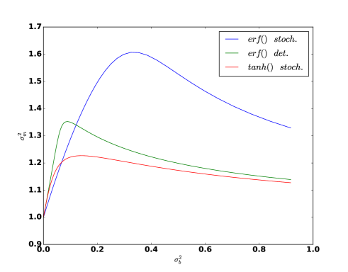
This can be established by rearranging Equations 13 and 15. We solve for σb2superscriptsubscript𝜎𝑏2\sigma_{b}^{2} numerically, as shown in Figure 3, for different neuron noise models and hence non-linearities φ()𝜑\varphi(\cdot). We find that the critical initialisation for any of these design choices is close to the point (σm2,σb2)=(1,0)superscriptsubscript𝜎𝑚2superscriptsubscript𝜎𝑏210(\sigma_{m}^{2},\sigma_{b}^{2})=(1,0). However, it is not just the singleton point, as for example in Hayou et al. (2019) for the ReLu case for standard networks. We plot the solutions in the Appendix.

3.2.2 Asymptotic expansions and depth scales

The depth scales, as derived in Schoenholz et al. (2016) provide a quantitative indicator to the number of layers correlations will survive for, and thus how trainable a network is. Similar depth scales can be derived for these deterministic surrogates. Asymptotically in network depth \ell, we expect that |qaaq|exp(ξq)similar-tosuperscriptsubscript𝑞𝑎𝑎superscript𝑞subscript𝜉𝑞|q_{aa}^{\ell}-q^{*}|\sim\exp(-\frac{\ell}{\xi_{q}}) and |cabc|exp(ξc)similar-tosubscriptsuperscript𝑐𝑎𝑏superscript𝑐subscript𝜉𝑐|c^{\ell}_{ab}-c^{*}|\sim\exp(-\frac{\ell}{\xi_{c}}), where the terms ξqsubscript𝜉𝑞\xi_{q} and ξcsubscript𝜉𝑐\xi_{c} define the depth scales over which the variance and correlations of signals may propagate. We are most interested in the correlation depth scale, since it relates to χ𝜒\chi. The derivation is identical to that of Schoenholz et al. (2016). One can expand the correlation cab=c+ϵsubscriptsuperscript𝑐𝑎𝑏superscript𝑐superscriptitalic-ϵc^{\ell}_{ab}=c^{*}+\epsilon^{\ell}, and assuming qaa=qsuperscriptsubscript𝑞𝑎𝑎superscript𝑞q_{aa}^{\ell}=q^{*}, it is possible to write

ϵ+1=ϵ[1+q1+σb2σm2Dzφ(u1)φ(u2)]+𝒪((ϵ)2)superscriptitalic-ϵ1superscriptitalic-ϵdelimited-[]1superscript𝑞1superscriptsubscript𝜎𝑏2subscriptsuperscript𝜎2𝑚𝐷𝑧superscript𝜑subscript𝑢1superscript𝜑subscript𝑢2𝒪superscriptsuperscriptitalic-ϵ2\displaystyle\epsilon^{\ell+1}=\epsilon^{\ell}\big{[}\frac{1+q^{*}}{1+\sigma_{b}^{2}}\sigma^{2}_{m}\int Dz\varphi^{\prime}(u_{1})\varphi^{\prime}(u_{2})\big{]}+\mathcal{O}((\epsilon^{\ell})^{2}) (16)

The depth scale ξc1superscriptsubscript𝜉𝑐1\xi_{c}^{-1} are given by the log ratio logϵ+1ϵsuperscriptitalic-ϵ1superscriptitalic-ϵ\log\frac{\epsilon^{\ell+1}}{\epsilon^{\ell}}.

ξc1superscriptsubscript𝜉𝑐1\displaystyle\xi_{c}^{-1} =log[1+q1+σb2σm2Dzφ(u1)φ(u2)]=logχabsent1superscript𝑞1superscriptsubscript𝜎𝑏2subscriptsuperscript𝜎2𝑚𝐷𝑧superscript𝜑subscript𝑢1superscript𝜑subscript𝑢2𝜒\displaystyle=-\log\big{[}\frac{1+q^{*}}{1+\sigma_{b}^{2}}\sigma^{2}_{m}\int Dz\varphi^{\prime}(u_{1})\varphi^{\prime}(u_{2})\big{]}=-\log\chi (17)

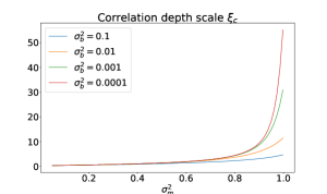
We plot this depth scale in Figure 2. We derive the variance depth scale in the appendices, since it is different to the standard continuous case, but not of prime practical importance.

3.3 Signal propagation theory for local reparameterization trick surrogates

From Equation 8, the pre-activation field for the perturbed surrogate with both stochastic binary weights and neurons is given by,

hi,alsuperscriptsubscript𝑖𝑎𝑙\displaystyle h_{i,a}^{l} =1NjMijlϕ(hj,al1)+bil+ϵi,a1Nj1(Mijl)2ϕ2(hj,al1)absent1𝑁subscript𝑗superscriptsubscript𝑀𝑖𝑗𝑙italic-ϕsuperscriptsubscript𝑗𝑎𝑙1superscriptsubscript𝑏𝑖𝑙superscriptsubscriptitalic-ϵ𝑖𝑎1𝑁subscript𝑗1superscriptsuperscriptsubscript𝑀𝑖𝑗𝑙2superscriptitalic-ϕ2superscriptsubscript𝑗𝑎𝑙1\displaystyle=\frac{1}{\sqrt{N}}\sum_{j}M_{ij}^{l}\phi(h_{j,a}^{l-1})+b_{i}^{l}+\epsilon_{i,a}^{\ell}\frac{1}{\sqrt{N}}\sqrt{\sum_{j}1-(M_{ij}^{l})^{2}\phi^{2}(h_{j,a}^{l-1})} (18)

where we recall that ϵ𝒩(0,1)similar-toitalic-ϵ𝒩01\epsilon\sim\mathcal{N}(0,1). The non-linearity ϕ()italic-ϕ\phi(\cdot) can of course be derived from any valid binary stochastic neuron model. Appealing to the same self-averaging arguments used in the previous section, we find the variance map to be

qaa=𝔼[(hi,al)2]superscriptsubscript𝑞𝑎𝑎𝔼delimited-[]superscriptsuperscriptsubscript𝑖𝑎𝑙2\displaystyle q_{aa}^{\ell}=\mathbb{E}\left[(h_{i,a}^{l})^{2}\right] =σm2𝔼ϕ2(hj,al1)+σb2+(1σm2𝔼ϕ2(hj,al1))=1+σb2absentsuperscriptsubscript𝜎𝑚2𝔼superscriptitalic-ϕ2superscriptsubscript𝑗𝑎𝑙1superscriptsubscript𝜎𝑏21superscriptsubscript𝜎𝑚2𝔼superscriptitalic-ϕ2superscriptsubscript𝑗𝑎𝑙11superscriptsubscript𝜎𝑏2\displaystyle=\sigma_{m}^{2}\mathbb{E}\phi^{2}(h_{j,a}^{l-1})+\sigma_{b}^{2}+(1-\sigma_{m}^{2}\mathbb{E}\phi^{2}(h_{j,a}^{l-1}))=1+\sigma_{b}^{2} (19)

Interestingly, we see that the variance map does not depend on the variance of the means of the binary weights. This is not immediately obvious from the pre-activation field definition. In the covariance map we do not have such a simplification since the perturbation ϵi,asubscriptitalic-ϵ𝑖𝑎\epsilon_{i,a} is uncorrelated between inputs a𝑎a and b𝑏b. Thus the correlation map is given by

cablsuperscriptsubscript𝑐𝑎𝑏𝑙\displaystyle c_{ab}^{l} =σm2𝔼ϕ(hj,al1)ϕ(hj,al1)+σb21+σb2absentsuperscriptsubscript𝜎𝑚2𝔼italic-ϕsuperscriptsubscript𝑗𝑎𝑙1italic-ϕsuperscriptsubscript𝑗𝑎𝑙1superscriptsubscript𝜎𝑏21superscriptsubscript𝜎𝑏2\displaystyle=\frac{\sigma_{m}^{2}\mathbb{E}\phi(h_{j,a}^{l-1})\phi(h_{j,a}^{l-1})+\sigma_{b}^{2}}{1+\sigma_{b}^{2}} (20)

3.4 Critical initialisation: LRT surrogates

Claim 2: There is no critical initialisation for the local reparameterisation trick based surrogate, for a network with binary weights and neurons.

Proof: The conditions for a critical initialisation are that c=1superscript𝑐1c^{*}=1 to be a fixed point and χ1=1subscript𝜒11\chi_{1}=1. No such fixed point exists. We have a fixed point c=1superscript𝑐1c^{*}=1 if and only if σm2=1/𝔼[ϕ2(hj,al1)]superscriptsubscript𝜎𝑚21𝔼delimited-[]superscriptitalic-ϕ2superscriptsubscript𝑗𝑎𝑙1\sigma_{m}^{2}=1/\mathbb{E}[\phi^{2}(h_{j,a}^{l-1})]. Note that σm21superscriptsubscript𝜎𝑚21\sigma_{m}^{2}\leq 1. For any ϕ(z)italic-ϕ𝑧\phi(z) which is the mean of the stochastic binary neuron, the expectation 𝔼[ϕ2(z)]1𝔼delimited-[]superscriptitalic-ϕ2𝑧1\mathbb{E}[\phi^{2}(z)]\leq 1. For example, consider ϕ(z)=tanh(κz)italic-ϕ𝑧𝜅𝑧\phi(z)=\tanh(\kappa z) for any finite kappa.

We also considered the LRT surrogate with continuous (tanh()\tanh(\cdot)) neurons and stochastic binary weights. The derivations are very similar to the previous case, as we show in the appendix. The variance and correlation maps are given by

qaa=𝔼ϕ2(hj,al1))+σb2cabl=σm2𝔼ϕ(hj,al1)ϕ(hj,al1)+σb2𝔼ϕ2(hj,al1)+σb2\displaystyle q_{aa}^{\ell}=\mathbb{E}\phi^{2}(h_{j,a}^{l-1}))+\sigma_{b}^{2}\qquad c_{ab}^{l}=\frac{\sigma_{m}^{2}\mathbb{E}\phi(h_{j,a}^{l-1})\phi(h_{j,a}^{l-1})+\sigma_{b}^{2}}{\mathbb{E}\phi^{2}(h_{j,a}^{l-1})+\sigma_{b}^{2}} (21)

This leads to the following result,

Claim 3: The critical initialisation for the LRT surrogate, for the case of continuous tanh()\tanh(\cdot) neurons and stochastic binary weights is the singleton (σb2,σm2)=(0,1)superscriptsubscript𝜎𝑏2superscriptsubscript𝜎𝑚201(\sigma_{b}^{2},\sigma_{m}^{2})=(0,1).

Proof: From the correlation map we have a fixed point c=1superscript𝑐1c^{*}=1 if and only if σm2=1superscriptsubscript𝜎𝑚21\sigma_{m}^{2}=1, by inspection. In turn, the critical initialisation condition χ1=1subscript𝜒11\chi_{1}=1 holds if 𝔼[(ϕ(hj,al1))2]=1σm2=1𝔼delimited-[]superscriptsuperscriptitalic-ϕsuperscriptsubscript𝑗𝑎𝑙121superscriptsubscript𝜎𝑚21\mathbb{E}[(\phi\ \!^{\prime}(h_{j,a}^{l-1}))^{2}]=\frac{1}{\sigma_{m}^{2}}=1. Thus, to find the critical initialisation, we need to find a value of qaa=𝔼ϕ2(hj,al1)+σb2subscript𝑞𝑎𝑎𝔼superscriptitalic-ϕ2superscriptsubscript𝑗𝑎𝑙1superscriptsubscript𝜎𝑏2q_{aa}=\mathbb{E}\phi^{2}(h_{j,a}^{l-1})+\sigma_{b}^{2} that satisfies this final condition. In the case that ϕ()=tanh()italic-ϕ\phi(\cdot)=\tanh(\cdot), then the function (ϕ(hj,al1))21superscriptsuperscriptitalic-ϕsuperscriptsubscript𝑗𝑎𝑙121(\phi\ \!^{\prime}(h_{j,a}^{l-1}))^{2}\leq 1, taking the value 111 at the origin only, this requires qaa0subscript𝑞𝑎𝑎0q_{aa}\to 0. Thus we have the singleton (σb2,σm2)=(0,1)superscriptsubscript𝜎𝑏2superscriptsubscript𝜎𝑚201(\sigma_{b}^{2},\sigma_{m}^{2})=(0,1) as the solution.

4 Numerical and experimental results

4.1 Simulations

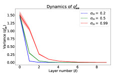
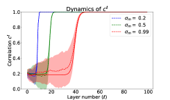
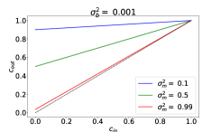
We first verify that the theory accurately predicts the average behaviour of randomly initialised networks. We present simulations for the deterministic surrogate in Figure 1. We see that the average behaviour of random networks are well predicted by the mean field theory. Estimates of the variance and correlation are plotted, with dotted lines corresponding to empirical means and the shaded area corresponding to one standard deviation. Theoretical predictions are given by solid lines, with strong agreement for even finite networks. Similar plots can be produced for the LRT surrogate. In Appendix D we plot the depth scales as functions of σmsubscript𝜎𝑚\sigma_{m} and σbsubscript𝜎𝑏\sigma_{b}.

Refer to caption
Refer to caption
Refer to caption
Figure 1: Dynamics of the variance and correlation maps, with simulations of a network of width N=1000𝑁1000N=1000, 50 realisations, for various hyperparameter settings: σm2{0.2,0.5,0.99}superscriptsubscript𝜎𝑚20.20.50.99\sigma_{m}^{2}\in\{0.2,0.5,0.99\} (blue, green and red respectively). (a) variance evolution, (b) correlation evolution. (c) correlation mapping (cinsubscript𝑐𝑖𝑛c_{in} to coutsubscript𝑐𝑜𝑢𝑡c_{out}), with σb2=0.001superscriptsubscript𝜎𝑏20.001\sigma_{b}^{2}=0.001

4.2 Training performance for different mean initialisation σm2superscriptsubscript𝜎𝑚2\sigma_{m}^{2}

Here we experimentally test the predictions of the mean field theory by training networks to overfit a dataset in the supervised learning setting, having arbitrary depth and different initialisations. We consider first the performance of the deterministic and LRT surrogates, not their corresponding binary networks.

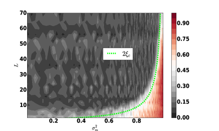
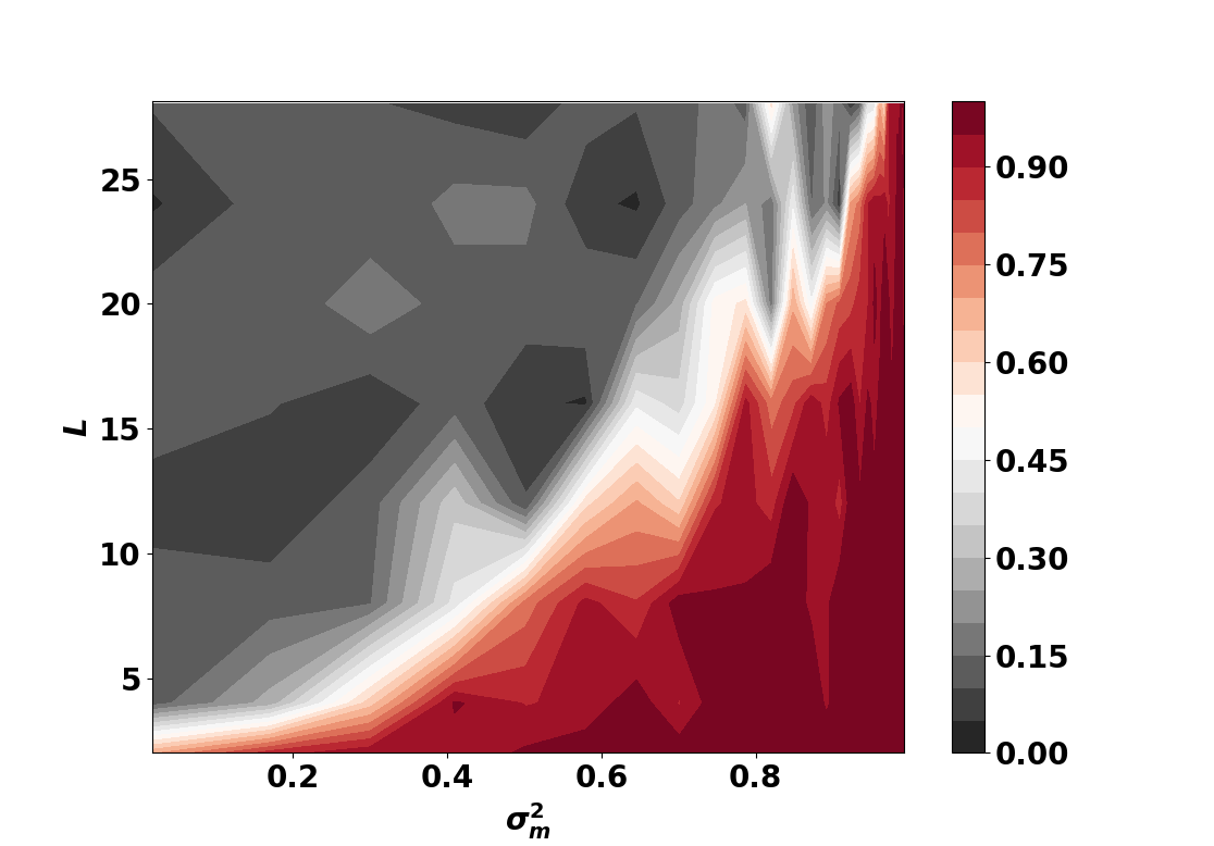
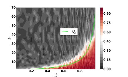
We use the MNIST dataset with reduced training set size (50%percent5050\%) and record the training performance (percentage of the training set correctly labeled) after 101010 epochs of gradient descent over the training set, for various network depths L<70𝐿70L<70 and different mean variances σm2[0,1)superscriptsubscript𝜎𝑚201\sigma_{m}^{2}\in[0,1). The optimizer used was SGD with Adam Kingma & Ba (2014) with a learning rate of 2×1042superscript1042\times 10^{-4} chosen after simple grid search, and a batch size of 646464. We see that the experimental results match the correlation depth scale derived, which are overlaid as dotted curves. A proportion of 3ξc3subscript𝜉𝑐3\xi_{c} was found to indicate the maximum attenuation in signal strength before trainability becomes difficult, similarly to previous works Schoenholz et al. (2016).

A reason we see the trainability not diverging in Figure 2 is that training time increases with depth, on top of requiring smaller learning rates for deeper networks, as described in Saxe et al. (2013). The experiment here used the same number of epochs regardless of depth, meaning shallower networks actually had an advantage over deeper networks. Note that the theory does not specify for how many steps of training the effects of critical initialisation will persist. Therefore, the number of steps we trained the network for is an arbitrary choice, and thus the experiments validate the theory in a more qualitative way. Results were similar for other optimizers, including SGD, SGD with momentum, and RMSprop. Note that these networks were trained without dropout, batchnorm or any other heuristics.

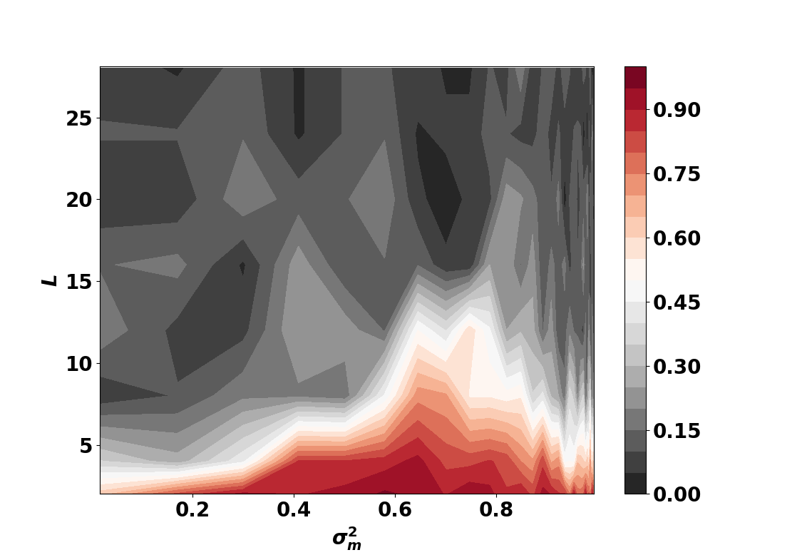
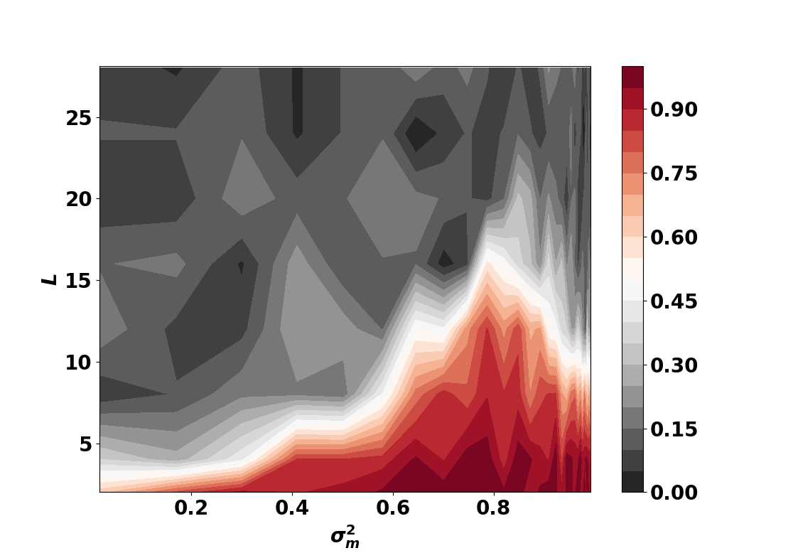
In Figure 2 we present the training performance for the deterministic surrogate and its stochastic binary counterpart. The results for a deterministic binary network were similar to a single Monte Carlo sample. Once again, we test our algorithms on the MNIST dataset and plot results after 555 epochs. We see that the performance of the stochastic network matches more closely the performance of the continuous surrogate as the number of samples increases, from N=5𝑁5N=5 to N=100𝑁100N=100 samples. We can report that the number of samples necessary to achieve better classification, at least for more shallow networks, appears to depends on the number of training epochs. This is a sensible relationship, since during the course of training we expect the means of the weights to polarise, moving closer to the bounds ±1plus-or-minus1\pm 1. Likewise, we expect that neurons, which initially have zero mean pre-activations, will also “saturate” during training, becoming either always “on” (+11+1) or “off” (11-1). A stochastic network being “closer” to deterministic would require fewer samples overall.
Refer to caption
Refer to caption
Refer to caption
(a)
Refer to caption
(b)
Refer to caption
(c)
Figure 2: Top: Training performance of the deterministic surrogate (left) and the LRT surrogate for stochastic binary weights and continuous neurons (right). The vertical axis represents network depth against the variance of the means σm2subscriptsuperscript𝜎2𝑚\sigma^{2}_{m}. Both surrogates were trained with σb2=0subscriptsuperscript𝜎2𝑏0\sigma^{2}_{b}=0. Thus, as σm21subscriptsuperscript𝜎2𝑚1\sigma^{2}_{m}\to 1 we approach criticality in both cases. Overlaid are curves proportional to the correlation depth scale ξcsubscript𝜉𝑐\xi_{c}. Bottom: Training performance of the deterministic surrogate and its binary counterparts after training on the MNIST dataset for 5 epochs. Left: performance of the continuous surrogate. Centre: the performance of the stochastic binary network, averaged over 5 Monte Carlo samples. Right: 100 Monte Carlo samples. The deterministic binary evaluation is similar to a single Monte Carlo sample, resembling the central figure.

5 Discussion

This study of two classes of surrogate networks, and the derivation of their initialisation theories has yielded results of practical significance. Based on the results of Section 3, in particular Claims 1-3, we can offer the following advice. If a practitioner is interested in training networks with binary weights and neurons, one should use the deterministic surrogate, not the LRT surrogate, since the latter has no critical initialisation. If a practitioner is interested in binary weights only,the LRT in this case does have a critical initialisation (and is the only choice from amongst these two classes of surrogate). Furthermore, both networks are critically initialised when σb20superscriptsubscript𝜎𝑏20\sigma_{b}^{2}\to 0 and by setting the means of the weights to ±1plus-or-minus1\pm 1.

It was seen that during training, when evaluating the stochastic binary counterparts concurrently with the surrogate, the performance of binary networks was worse than the continuous model, especially as depth increases. We reported that the stochastic binary network, with more samples, outperformed the deterministic binary network, a reasonable result since the objective optimised is the expectation over an ensemble of stochastic binary networks.

A study of random deterministic binary networks, included in the Appendices, and published recently Blumenfeld et al. (2019) for a different problem, reveals unsurprisingly that binary networks are always in a chaotic phase. However a binary network which is trained via some algorithm will of course have different signal propagation behaviour. It makes sense that the closer one is to the early stages of the training process, the closer the signal propagation behaviour is to the randomly initialised case. We might expect that as training progresses the behaviour of the binary counterparts approaches that of the trained surrogate. Any such difference would not be observed for a heuristic surrogate as used in Courbariaux & Bengio (2016) or Rastegari et al. (2016), which has no continuous forward propagation equations.

References

  • Baldassi et al. (2018) Carlo Baldassi, Federica Gerace, Hilbert J. Kappen, Carlo Lucibello, Luca Saglietti, Enzo Tartaglione, and Riccardo Zecchina. Role of synaptic stochasticity in training low-precision neural networks. Phys. Rev. Lett., 120:268103, Jun 2018. doi: 10.1103/PhysRevLett.120.268103. URL https://link.aps.org/doi/10.1103/PhysRevLett.120.268103.
  • Bengio et al. (2013) Yoshua Bengio, Nicholas Léonard, and Aaron Courville. Estimating or propagating gradients through stochastic neurons for conditional computation, 2013.
  • Blumenfeld et al. (2019) Yaniv Blumenfeld, Dar Gilboa, and Daniel Soudry. A mean field theory of quantized deep networks: The quantization-depth trade-off. In H. Wallach, H. Larochelle, A. Beygelzimer, F. d. Alche-Buc, E. Fox, and R. Garnett (eds.), Advances in Neural Information Processing Systems 32, pp.  7038–7048. Curran Associates, Inc., 2019.
  • Courbariaux & Bengio (2016) Matthieu Courbariaux and Yoshua Bengio. Binarynet: Training deep neural networks with weights and activations constrained to +1 or -1. CoRR, abs/1602.02830, 2016. URL http://arxiv.org/abs/1602.02830.
  • Glorot & Bengio (2010) Xavier Glorot and Yoshua Bengio. Understanding the difficulty of training deep feedforward neural networks. In Yee Whye Teh and Mike Titterington (eds.), Proceedings of the Thirteenth International Conference on Artificial Intelligence and Statistics, volume 9 of Proceedings of Machine Learning Research, pp.  249–256, Chia Laguna Resort, Sardinia, Italy, 13–15 May 2010. PMLR. URL http://proceedings.mlr.press/v9/glorot10a.html.
  • Hayou et al. (2019) Soufiane Hayou, Arnaud Doucet, and Judith Rousseau. On the impact of the activation function on deep neural networks training. In Kamalika Chaudhuri and Ruslan Salakhutdinov (eds.), Proceedings of the 36th International Conference on Machine Learning, volume 97 of Proceedings of Machine Learning Research, pp. 2672–2680, Long Beach, California, USA, 09–15 Jun 2019. PMLR. URL http://proceedings.mlr.press/v97/hayou19a.html.
  • Kingma & Ba (2014) Diederik P. Kingma and Jimmy Ba. Adam: A method for stochastic optimization. CoRR, abs/1412.6980, 2014. URL http://arxiv.org/abs/1412.6980.
  • Kingma & Welling (2013) Diederik P. Kingma and Max Welling. Auto-encoding variational bayes. CoRR, abs/1312.6114, 2013.
  • Mezard et al. (1987) Marc Mezard, Giorgio Parisi, and Miguel Virasoro. Spin Glass Theory and Beyond, volume 9. 01 1987. doi: 10.1063/1.2811676.
  • Peters & Welling (2018) Jorn W. T. Peters and Max Welling. Probabilistic binary neural networks. CoRR, abs/1809.03368, 2018. URL http://arxiv.org/abs/1809.03368.
  • Poole et al. (2016) Ben Poole, Subhaneil Lahiri, Maithra Raghu, Jascha Sohl-Dickstein, and Surya Ganguli. Exponential expressivity in deep neural networks through transient chaos. In D. D. Lee, M. Sugiyama, U. V. Luxburg, I. Guyon, and R. Garnett (eds.), Advances in Neural Information Processing Systems 29, pp. 3360–3368. Curran Associates, Inc., 2016.
  • Rastegari et al. (2016) Mohammad Rastegari, Vicente Ordonez, Joseph Redmon, and Ali Farhadi. Xnor-net: Imagenet classification using binary convolutional neural networks. In Bastian Leibe, Jiri Matas, Nicu Sebe, and Max Welling (eds.), European Conference on Computer Vision, pp.  525–542, Cham, 2016. Springer International Publishing.
  • Saxe et al. (2013) Andrew M. Saxe, James L. McClelland, and Surya Ganguli. Exact solutions to the nonlinear dynamics of learning in deep linear neural networks. CoRR, abs/1312.6120, 2013. URL http://arxiv.org/abs/1312.6120.
  • Schoenholz et al. (2016) Samuel S. Schoenholz, Justin Gilmer, Surya Ganguli, and Jascha Sohl-Dickstein. Deep information propagation. CoRR, abs/1611.01232, 2016. URL http://arxiv.org/abs/1611.01232.
  • Shayer et al. (2017) Oran Shayer, Dan Levi, and Ethan Fetaya. Learning discrete weights using the local reparameterization trick. CoRR, abs/1710.07739, 2017. URL http://arxiv.org/abs/1710.07739.
  • Soudry et al. (2014) Daniel Soudry, Itay Hubara, and Ron Meir. Expectation backpropagation: Parameter-free training of multilayer neural networks with continuous or discrete weights. In Z. Ghahramani, M. Welling, C. Cortes, N. D. Lawrence, and K. Q. Weinberger (eds.), Advances in Neural Information Processing Systems 27, pp.  963–971. Curran Associates, Inc., 2014.

Appendix A Derivation of deterministic surrogate networks

A.1 Integrating over stochastic or deterministic binary neurons

The form of each neuron’s probability distribution depends on the underlying noise model. We can express a stochastic binary random variable 𝐒{±1}𝐒plus-or-minus1{\bf S}\in\{\pm 1\} with 𝐒p(𝐒;θ)similar-to𝐒𝑝𝐒𝜃{\bf S}\sim p({\bf S};\theta) via its latent variable formulation,

𝐒=sign(θ+α𝐋)𝐒sign𝜃𝛼𝐋\displaystyle{\bf S}=\operatorname{sign}(\theta+\alpha\mathbf{L}) (22)

In this form θ𝜃\theta is referred to as a “natural” parameter, from the statistics literature on exponential families. The term 𝐋𝐋\mathbf{L} is a latent random noise, which determines the form of the probability distribution. We also introduce a scaling α𝛼\alpha to control the variance of the noise, so that as α0𝛼0\alpha\to 0 the neuron becomes a deterministic sign function. Letting α=1𝛼1\alpha=1 for simplicity, we see that the probability of the binary variable taking a positive value is

p(𝐒=+1)=θp(𝐋)𝑑𝐋𝑝𝐒1superscriptsubscript𝜃𝑝𝐋differential-d𝐋\displaystyle p({\bf S}=+1)=\int_{-\infty}^{-\theta}p(\mathbf{L})d\mathbf{L} (23)

where p(𝐋)𝑝𝐋p(\mathbf{L}) is the known probability density function for the noise 𝐋𝐋\mathbf{L}. The two common choices of noise models are Gaussian or logistic noise. The Gaussian of course has shifted and scaled erf()erf\operatorname{erf}(\cdot) function as its cumulative distribution. The logistic random variable has the classic “sigmoid” or logistic function as its CDF, σ(z)=11+ez𝜎𝑧11superscript𝑒𝑧\sigma(z)=\frac{1}{1+e^{-z}}.

Thus, the probability of a the variable being positive is a function of the CDF. In the Gaussian case, this is Φ(θ)Φ𝜃\Phi(\theta). By symmetry, the probability of p(𝐒=1)=Φ(θ)𝑝𝐒1Φ𝜃p({\bf S}=-1)=\Phi(-\theta). Thus, we see the probability distribution for the binary random variable in general is the CDF of the noise 𝐋𝐋\mathbf{L}, and we write p(𝐒)=Φ(𝐒θ)𝑝𝐒Φ𝐒𝜃p({\bf S})=\Phi({\bf S}\theta). In the logistic noise case, we have p(𝐒)=σ(𝐒θ)𝑝𝐒𝜎𝐒𝜃p({\bf S})=\sigma({\bf S}\theta)

For the stochastic neurons, the natural parameter is the incoming field 𝐡i=j𝐒i,j𝐱j1+bisubscriptsuperscript𝐡𝑖subscript𝑗subscriptsuperscript𝐒𝑖𝑗subscriptsuperscript𝐱1𝑗subscriptsuperscript𝑏𝑖{\bf h}^{\ell}_{i}=\sum_{j}{\bf S}^{\ell}_{i,j}{\bf x}^{\ell-1}_{j}+b^{\ell}_{i}. Assuming this is approximately Gaussian in the large layer width limit, we can successively marginalise over the stochastic inputs to each neuron, calculating an approximation of each neuron’s probability distribution, p^(𝐱i)^𝑝subscriptsuperscript𝐱𝑖\hat{p}({\bf x}^{\ell}_{i}). This approximation is then used in the central limit theorem for the next layer, and so on.

For the case of neurons with latent Gaussian noise as part of the binary random variable model, the integration over the pre-activation field (assumed to be Gaussian) is exact. Explicitly,

p(𝐱i)𝑝subscriptsuperscript𝐱𝑖\displaystyle p({\bf x}^{\ell}_{i}) =𝐱1𝐒p(𝐱i|𝐱1,𝐒)p(𝐒1)p^(𝐱)absentsubscriptsuperscript𝐱1subscriptsuperscript𝐒𝑝conditionalsubscriptsuperscript𝐱𝑖superscript𝐱1superscript𝐒𝑝superscript𝐒1^𝑝superscript𝐱\displaystyle=\sum_{{\bf x}^{\ell-1}}\sum_{{\bf S}^{\ell}}p({\bf x}^{\ell}_{i}|{\bf x}^{\ell-1},{\bf S}^{\ell})p({\bf S}^{\ell-1})\hat{p}({\bf x}^{\ell})
Φ(𝐱i𝐡i)𝒩(𝐡i|h¯i,(ΣMF)ii)absentΦsubscriptsuperscript𝐱𝑖subscriptsuperscript𝐡𝑖𝒩conditionalsubscriptsuperscript𝐡𝑖superscriptsubscript¯𝑖subscriptsuperscriptsubscriptΣ𝑀𝐹𝑖𝑖\displaystyle\approx\int\Phi({\bf x}^{\ell}_{i}{\bf h}^{\ell}_{i})\mathcal{N}({\bf h}^{\ell}_{i}|\bar{h}_{i}^{\ell},(\Sigma_{MF}^{\ell})_{ii})
=Φ(h¯i1+2(ΣMF)ii𝐱i)=p^(𝐱i)absentΦsuperscriptsubscript¯𝑖12subscriptsuperscriptsubscriptΣ𝑀𝐹𝑖𝑖subscriptsuperscript𝐱𝑖^𝑝subscriptsuperscript𝐱𝑖\displaystyle=\Phi\bigg{(}\frac{\bar{h}_{i}^{\ell}}{\sqrt{1+2(\Sigma_{MF}^{\ell})_{ii}}}{\bf x}^{\ell}_{i}\bigg{)}=\hat{p}({\bf x}^{\ell}_{i}) (24)

where Φ()Φ\Phi(\cdot) is the CDF of the Gaussian distribution. We have again ΣMFsubscriptΣ𝑀𝐹\Sigma_{MF} denoting the mean field approximation to the covariance between the stochastic binary pre-activations. The Gaussian expectation of the Gaussian CDF is a known identity, which we state in more generality in the next section, where we also consider neurons with logistic noise.

This new approximate probability distribution p^(𝐱i)^𝑝subscriptsuperscript𝐱𝑖\hat{p}({\bf x}^{\ell}_{i}) can then used as part of the Gaussian CLT applied at the next layer, since it determines the means of the neurons in the next layer,

𝔼𝐱i=2Φ(h¯i1+(ΣMF)ii)1𝔼subscriptsuperscript𝐱𝑖2Φsuperscriptsubscript¯𝑖1subscriptsuperscriptsubscriptΣ𝑀𝐹𝑖𝑖1\displaystyle\mathbb{E}{\bf x}^{\ell}_{i}=2\Phi\bigg{(}\frac{\bar{h}_{i}^{\ell}}{\sqrt{1+(\Sigma_{MF}^{\ell})_{ii}}}\bigg{)}-1 (25)

If we follow these setps from layer to layer, we see that we are actually propagating approximate means for the neurons, combined non-linearly with the means of the weights. Given the approximately analytically integrated loss function, it is possible to perform gradient descent with respect to the means and biases, Mijsuperscriptsubscript𝑀𝑖𝑗M_{ij}^{\ell} and bisubscriptsuperscript𝑏𝑖b^{\ell}_{i}.

In the case of deterministic sign()sign\operatorname{sign}() neurons we obtain particularly simple expressions. In this case the “probability” of a neuron taking, for instance, positive is just Heaviside step function of the incoming field. Denoting the Heaviside with Θ()Θ\Theta(\cdot), we have

p(𝐱i)𝑝subscriptsuperscript𝐱𝑖\displaystyle p({\bf x}^{\ell}_{i}) =𝐱1𝐒p(𝐱i|𝐱1,𝐒)p(𝐒1)p^(𝐱1)absentsubscriptsuperscript𝐱1subscriptsuperscript𝐒𝑝conditionalsubscriptsuperscript𝐱𝑖superscript𝐱1superscript𝐒𝑝superscript𝐒1^𝑝superscript𝐱1\displaystyle=\sum_{{\bf x}^{\ell-1}}\sum_{{\bf S}^{\ell}}p({\bf x}^{\ell}_{i}|{\bf x}^{\ell-1},{\bf S}^{\ell})p({\bf S}^{\ell-1})\hat{p}({\bf x}^{\ell-1})
Θ(𝐱i𝐡i)𝒩(𝐡i|h¯i,(ΣMF)ii)absentΘsubscriptsuperscript𝐱𝑖subscriptsuperscript𝐡𝑖𝒩conditionalsubscriptsuperscript𝐡𝑖superscriptsubscript¯𝑖subscriptsuperscriptsubscriptΣ𝑀𝐹𝑖𝑖\displaystyle\approx\int\Theta({\bf x}^{\ell}_{i}{\bf h}^{\ell}_{i})\mathcal{N}({\bf h}^{\ell}_{i}|\bar{h}_{i}^{\ell},(\Sigma_{MF}^{\ell})_{ii})
Φ(h¯i(ΣMF)ii12𝐱i)=p^(𝐱i)absentΦsuperscriptsubscript¯𝑖subscriptsuperscriptsuperscriptsubscriptΣ𝑀𝐹12𝑖𝑖subscriptsuperscript𝐱𝑖^𝑝subscriptsuperscript𝐱𝑖\displaystyle\approx\Phi\bigg{(}\frac{\bar{h}_{i}^{\ell}}{(\Sigma_{MF}^{\ell})^{-\frac{1}{2}}_{ii}}{\bf x}^{\ell}_{i}\bigg{)}=\hat{p}({\bf x}^{\ell}_{i}) (26)

We can write out the network forward equations for the case of deterministic binary neurons, since it is a particularly elegant result. In general we have

x¯i=ϕ(ηh),h=ΣMFh¯,h¯=Mx1+bformulae-sequencesubscriptsuperscript¯𝑥𝑖italic-ϕ𝜂superscriptformulae-sequencesuperscriptsubscriptΣ𝑀𝐹superscript¯superscript¯superscript𝑀superscript𝑥1superscript𝑏\displaystyle\bar{x}^{\ell}_{i}=\phi(\eta\ \!h^{\ell}),\quad h^{\ell}\!=\sqrt{\Sigma_{MF}}\bar{h}^{\ell},\quad\bar{h}^{\ell}=M^{\ell}x^{\ell-1}+b^{\ell} (27)

where ϕ()=erf()italic-ϕerf\phi(\cdot)=\operatorname{erf}(\cdot) is the mean of the next layer of neurons, being a scaled and shifted version of the neuron’s noise model CDF. The constant is η=12𝜂12\eta=\frac{1}{\sqrt{2}}, standard for the Gaussian CDF to error functin conversion.

A.2 Exact and approximate Gaussian integration of sigmoidal functions

We now present the integration of stochastic neurons with logistic as well as Gaussian noise as part of their latent variable models. The logistic case is an approximation built on the Gaussian case, motivated by approximating the logistic CDF with the Gaussian CDF. The reason we may be interested in using logistic CDFs, rather than just considering latent Gaussian noise models which integrate exactly, is not justified in any rigorous or experimental way. Any such analysis would likely consider the effect of the tails of the logistic versus the Gaussian distributions, where the logistic tails are much heavier than those of the Gaussian. One historic reason for considering the logistic function, we note, is the prevalence of logistic-type functions (such as tanh()\tanh(\cdot)) in the neural network literature. The computational cost of evaluating either logistic or error functions is similar, so there is no motivation from the efficiency side. Instead it seems a historic preference to have logistic type functions used with neural networks.

As we saw in the previous subsection, the integration over the analytic probability distribution for each neuron gave a function which allows us to calculate the means of the neurons in the next layer. Therefore, we directly calculate the expression for the means.

The Gaussian integral of the Gaussian CDF was used in the previous section to derive the exact probability distribution for the stochastic binary neuron in the next layer. The result is well known, and can be stated in generality as follows,

Φ(ay)e(yx)22σ22πσ2𝑑y=Φ(x1+a2σ2)superscriptsubscriptΦ𝑎𝑦superscript𝑒superscript𝑦𝑥22superscript𝜎22𝜋superscript𝜎2differential-d𝑦Φ𝑥1superscript𝑎2superscript𝜎2\displaystyle\int_{-\infty}^{\infty}\Phi(ay)\frac{e^{-\frac{(y-x)^{2}}{2\sigma^{2}}}}{\sqrt{2\pi\sigma^{2}}}dy=\Phi(\frac{x}{\sqrt{1+a^{2}\sigma^{2}}}) (28)

We can integrate a logistic noise binary neuron using this result as well. The idea is to approximate the logistic noise with a suitably scaled Gaussian noise. However, since the overall network approximation results in propagating means from layer to layer, we can equivalently need to approximate the tanh()\tanh(\cdot) with the with the erferf\operatorname{erf}. Specifically, if we have f(x;α)=tanh(xα)𝑓𝑥𝛼𝑥𝛼f(x;\alpha)=\tanh(\frac{x}{\alpha}), an approximation is g(x;α)=erf(π2αx)𝑔𝑥𝛼erf𝜋2𝛼𝑥g(x;\alpha)=\operatorname{erf}(\frac{\sqrt{\pi}}{2\alpha}x), by requiring equality of derivatives at the origin. In order to establish this, consider

f(0;α)superscript𝑓0𝛼\displaystyle f^{\prime}(0;\alpha) =(1tanh2(0/α)1α=1α\displaystyle=(1-\tanh^{2}(0/\alpha)\frac{1}{\alpha}=\frac{1}{\alpha} (29)

and

derf(x;σ)dx|x=0evaluated-at𝑑erf𝑥𝜎𝑑𝑥𝑥0\displaystyle\frac{d\operatorname{erf}(x;\sigma)}{dx}|_{x=0} =2πσ2ex2/σ2|x=0=2πσ2absentevaluated-at2𝜋superscript𝜎2superscript𝑒superscript𝑥2superscript𝜎2𝑥02𝜋superscript𝜎2\displaystyle=\frac{2}{\sqrt{\pi\sigma^{2}}}e^{-x^{2}/\sigma^{2}}|_{x=0}=\frac{2}{\sqrt{\pi\sigma^{2}}} (30)

Equating these, gives σ2=4α2πsuperscript𝜎24superscript𝛼2𝜋\sigma^{2}=\frac{4\alpha^{2}}{\pi}, thus σ=2απ𝜎2𝛼𝜋\sigma=\frac{2\alpha}{\sqrt{\pi}}.

The approximate integral over the stochastic binary neuron mean is then

f(y;α)e(yx)22σ22πσ2𝑑ysuperscriptsubscript𝑓𝑦𝛼superscript𝑒superscript𝑦𝑥22superscript𝜎22𝜋superscript𝜎2differential-d𝑦\displaystyle\int_{-\infty}^{\infty}f(y;\alpha)\frac{e^{-\frac{(y-x)^{2}}{2\sigma^{2}}}}{\sqrt{2\pi\sigma^{2}}}dy erf(π2αy)e(yx)22σ22πσ2𝑑yabsentsuperscriptsubscripterf𝜋2𝛼𝑦superscript𝑒superscript𝑦𝑥22superscript𝜎22𝜋superscript𝜎2differential-d𝑦\displaystyle\approx\int_{-\infty}^{\infty}\operatorname{erf}(\frac{\sqrt{\pi}}{2\alpha}y)\frac{e^{-\frac{(y-x)^{2}}{2\sigma^{2}}}}{\sqrt{2\pi\sigma^{2}}}dy (31)
=erf(π2αγx)absenterf𝜋2𝛼𝛾𝑥\displaystyle=\operatorname{erf}(\frac{\sqrt{\pi}}{2\alpha\gamma}x) (32)
with γ=1+πσ22α2with 𝛾1𝜋superscript𝜎22superscript𝛼2\displaystyle\text{with }\gamma=\sqrt{1+\frac{\pi\sigma^{2}}{2\alpha^{2}}} (33)

If we so desire, we can approximate this again with a tanh()\tanh(\cdot) using the tanh()\tanh(\cdot) to erf()erf\operatorname{erf}(\cdot) approximation in reverse. The scale parameter of this tanh()\tanh(\cdot) will be α2=π4αγsubscript𝛼2𝜋4𝛼𝛾\alpha_{2}=\frac{\pi}{4\alpha\gamma}. If α=1𝛼1\alpha=1 as is standard, then

erf(π2γx)tanh(πx4γ)erf𝜋2𝛾𝑥𝜋𝑥4𝛾\displaystyle\operatorname{erf}(\frac{\sqrt{\pi}}{2\gamma}x)\approx\tanh(\frac{\pi x}{4\gamma}) (34)

Appendix B Equivalence of deterministic and stochastic neurons for deterministic surrogate

Assume a stochastic neuron with some latent noise, as per the previous appendix, with mean x¯i=𝔼p(xi)xi=ϕ(hi1)subscriptsuperscript¯𝑥𝑖subscript𝔼𝑝subscript𝑥𝑖subscriptsuperscript𝑥𝑖italic-ϕsubscriptsuperscript1𝑖\bar{x}^{\ell}_{i}=\mathbb{E}_{p(x_{i})}x^{\ell}_{i}=\phi(h^{\ell-1}_{i}). The field is given by

hi=12jMijϕ(hi1)+bi1+2j[1(Mij)2ϕ2(hi1)]superscriptsubscript𝑖12subscript𝑗superscriptsubscript𝑀𝑖𝑗italic-ϕsubscriptsuperscript1𝑖superscriptsubscript𝑏𝑖12subscript𝑗delimited-[]1superscriptsuperscriptsubscript𝑀𝑖𝑗2superscriptitalic-ϕ2subscriptsuperscript1𝑖\displaystyle h_{i}^{\ell}=\frac{1}{\sqrt{2}}\frac{\sum_{j}M_{ij}^{\ell}\phi(h^{\ell-1}_{i})+b_{i}^{\ell}}{\sqrt{1+2\sum_{j}[1-(M_{ij}^{\ell})^{2}\phi^{2}(h^{\ell-1}_{i})]}} (35)

We see that the expression for the variance of the field simplifies as follows,

qaa=𝔼(hi)2superscriptsubscript𝑞𝑎𝑎𝔼superscriptsuperscriptsubscript𝑖2\displaystyle q_{aa}^{\ell}=\mathbb{E}(h_{i}^{\ell})^{2} =12jMijϕ(hi1)+bi1+2j[1(Mij)2ϕ2(hi1)]absent12subscript𝑗superscriptsubscript𝑀𝑖𝑗italic-ϕsubscriptsuperscript1𝑖superscriptsubscript𝑏𝑖12subscript𝑗delimited-[]1superscriptsuperscriptsubscript𝑀𝑖𝑗2superscriptitalic-ϕ2subscriptsuperscript1𝑖\displaystyle=\frac{1}{2}\frac{\sum_{j}M_{ij}^{\ell}\phi(h^{\ell-1}_{i})+b_{i}^{\ell}}{1+2\sum_{j}[1-(M_{ij}^{\ell})^{2}\phi^{2}(h^{\ell-1}_{i})]} (36)
=12N(σm2𝔼ϕ2(hj,al1)+σb2)1+2(NNσm2𝔼ϕ2(hj,al1))absent12𝑁superscriptsubscript𝜎𝑚2𝔼superscriptitalic-ϕ2superscriptsubscript𝑗𝑎𝑙1superscriptsubscript𝜎𝑏212𝑁𝑁superscriptsubscript𝜎𝑚2𝔼superscriptitalic-ϕ2superscriptsubscript𝑗𝑎𝑙1\displaystyle=\frac{1}{2}\frac{N(\sigma_{m}^{2}\mathbb{E}\phi^{2}(h_{j,a}^{l-1})+\sigma_{b}^{2})}{1+2(N-N\sigma_{m}^{2}\mathbb{E}\phi^{2}(h_{j,a}^{l-1}))} (37)
=12σm2𝔼ϕ2(hj,al1)+σb22(1σm2𝔼ϕ2(hj,al1))absent12superscriptsubscript𝜎𝑚2𝔼superscriptitalic-ϕ2superscriptsubscript𝑗𝑎𝑙1superscriptsubscript𝜎𝑏221superscriptsubscript𝜎𝑚2𝔼superscriptitalic-ϕ2superscriptsubscript𝑗𝑎𝑙1\displaystyle=\frac{1}{2}\frac{\sigma_{m}^{2}\mathbb{E}\phi^{2}(h_{j,a}^{l-1})+\sigma_{b}^{2}}{2(1-\sigma_{m}^{2}\mathbb{E}\phi^{2}(h_{j,a}^{l-1}))} (38)

By similar steps, we find that in the deterministic binary neuron case, we would obtain the same expression, albeit with a different scaling constant. This is easily seen by inspection of the field term in the deterministic neuron case,

hi=12jMijϕ(hi1)+bij[1(Mij)2ϕ2(hi1)]superscriptsubscript𝑖12subscript𝑗superscriptsubscript𝑀𝑖𝑗italic-ϕsubscriptsuperscript1𝑖superscriptsubscript𝑏𝑖subscript𝑗delimited-[]1superscriptsuperscriptsubscript𝑀𝑖𝑗2superscriptitalic-ϕ2subscriptsuperscript1𝑖\displaystyle h_{i}^{\ell}=\frac{1}{\sqrt{2}}\frac{\sum_{j}M_{ij}^{\ell}\phi(h^{\ell-1}_{i})+b_{i}^{\ell}}{\sqrt{\sum_{j}[1-(M_{ij}^{\ell})^{2}\phi^{2}(h^{\ell-1}_{i})]}} (39)

which again was derived in the previous appendix.

Appendix C Derivation of signal propagation equations in deterministic surrogate networks

Here we present the derivations for the signal propagation in the continuous network models studied in the paper.

C.1 Variance propagation

We first calculate the variance given a signal:

qaal=1Nli(hi,al)2=E[(hi,al)2]superscriptsubscript𝑞𝑎𝑎𝑙1subscript𝑁𝑙subscript𝑖superscriptsuperscriptsubscript𝑖𝑎𝑙2𝐸delimited-[]superscriptsuperscriptsubscript𝑖𝑎𝑙2\displaystyle q_{aa}^{l}=\frac{1}{N_{l}}\sum_{i}\left(h_{i,a}^{l}\right)^{2}=E\left[\left(h_{i,a}^{l}\right)^{2}\right] (40)

Where for us:

hi,al=jmijlϕ(hj,al1)+bilj(1(mijl)2ϕ2(hj,al1))superscriptsubscript𝑖𝑎𝑙subscript𝑗superscriptsubscript𝑚𝑖𝑗𝑙italic-ϕsuperscriptsubscript𝑗𝑎𝑙1superscriptsubscript𝑏𝑖𝑙subscript𝑗1superscriptsuperscriptsubscript𝑚𝑖𝑗𝑙2superscriptitalic-ϕ2superscriptsubscript𝑗𝑎𝑙1\displaystyle h_{i,a}^{l}=\frac{\sum_{j}m_{ij}^{l}\phi\left(h_{j,a}^{l-1}\right)+b_{i}^{l}}{\sqrt{\sum_{j}\left(1-\left(m_{ij}^{l}\right)^{2}\phi^{2}\left(h_{j,a}^{l-1}\right)\right)}} (41)

and

mijN(0,σm2)biN(0,Nl1σb2)similar-tosubscript𝑚𝑖𝑗𝑁0superscriptsubscript𝜎𝑚2subscript𝑏𝑖similar-to𝑁0subscript𝑁𝑙1superscriptsubscript𝜎𝑏2\displaystyle m_{ij}\sim N\left(0,\sigma_{m}^{2}\right)b_{i}\sim N\left(0,N_{l-1}\sigma_{b}^{2}\right) (42)
𝔼[(hi,al)2]𝔼delimited-[]superscriptsuperscriptsubscript𝑖𝑎𝑙2\displaystyle\mathbb{E}\left[\left(h_{i,a}^{l}\right)^{2}\right] =𝔼[(jmijlϕ(hj,al1)+bilj(1(mijl)2ϕ2(hj,al1)))2]=𝔼[(jmijlϕ(hj,al1)+bil)2]Nl1j(mijl)2ϕ2(hj,al1)absent𝔼delimited-[]superscriptsubscript𝑗superscriptsubscript𝑚𝑖𝑗𝑙italic-ϕsuperscriptsubscript𝑗𝑎𝑙1superscriptsubscript𝑏𝑖𝑙subscript𝑗1superscriptsuperscriptsubscript𝑚𝑖𝑗𝑙2superscriptitalic-ϕ2superscriptsubscript𝑗𝑎𝑙12𝔼delimited-[]superscriptsubscript𝑗superscriptsubscript𝑚𝑖𝑗𝑙italic-ϕsuperscriptsubscript𝑗𝑎𝑙1superscriptsubscript𝑏𝑖𝑙2subscript𝑁𝑙1subscript𝑗superscriptsuperscriptsubscript𝑚𝑖𝑗𝑙2superscriptitalic-ϕ2superscriptsubscript𝑗𝑎𝑙1\displaystyle=\mathbb{E}\left[\left(\frac{\sum_{j}m_{ij}^{l}\phi\left(h_{j,a}^{l-1}\right)+b_{i}^{l}}{\sqrt{\sum_{j}\left(1-\left(m_{ij}^{l}\right)^{2}\phi^{2}\left(h_{j,a}^{l-1}\right)\right)}}\right)^{2}\right]=\frac{\mathbb{E}\left[\left(\sum_{j}m_{ij}^{l}\phi\left(h_{j,a}^{l-1}\right)+b_{i}^{l}\right)^{2}\right]}{N_{l-1}-\sum_{j}\left(m_{ij}^{l}\right)^{2}\phi^{2}\left(h_{j,a}^{l-1}\right)}
=jσm2𝔼ϕ2(hj,al1)+Nl1σb2Nl1(11Nl1j(mijl)2ϕ2(hj,al1))=Nl1σm2𝔼ϕ2(hj,al1)+Nl1σb2Nl1(1σm2𝔼ϕ2(hj,al1))absentsubscript𝑗superscriptsubscript𝜎𝑚2𝔼superscriptitalic-ϕ2superscriptsubscript𝑗𝑎𝑙1subscript𝑁𝑙1superscriptsubscript𝜎𝑏2subscript𝑁𝑙111subscript𝑁𝑙1subscript𝑗superscriptsuperscriptsubscript𝑚𝑖𝑗𝑙2superscriptitalic-ϕ2superscriptsubscript𝑗𝑎𝑙1subscript𝑁𝑙1superscriptsubscript𝜎𝑚2𝔼superscriptitalic-ϕ2superscriptsubscript𝑗𝑎𝑙1subscript𝑁𝑙1superscriptsubscript𝜎𝑏2subscript𝑁𝑙11superscriptsubscript𝜎𝑚2𝔼superscriptitalic-ϕ2superscriptsubscript𝑗𝑎𝑙1\displaystyle=\frac{\sum_{j}\sigma_{m}^{2}\mathbb{E}\phi^{2}\left(h_{j,a}^{l-1}\right)+N_{l-1}\sigma_{b}^{2}}{N_{l-1}\left(1-\frac{1}{N_{l-1}}\sum_{j}\left(m_{ij}^{l}\right)^{2}\phi^{2}\left(h_{j,a}^{l-1}\right)\right)}=\frac{N_{l-1}\sigma_{m}^{2}\mathbb{E}\phi^{2}\left(h_{j,a}^{l-1}\right)+N_{l-1}\sigma_{b}^{2}}{N_{l-1}\left(1-\sigma_{m}^{2}\mathbb{E}\phi^{2}\left(h_{j,a}^{l-1}\right)\right)}
=σm2𝔼ϕ2(hj,al1)+σb21σm2𝔼ϕ2(hj,al1)absentsuperscriptsubscript𝜎𝑚2𝔼superscriptitalic-ϕ2superscriptsubscript𝑗𝑎𝑙1superscriptsubscript𝜎𝑏21superscriptsubscript𝜎𝑚2𝔼superscriptitalic-ϕ2superscriptsubscript𝑗𝑎𝑙1\displaystyle=\frac{\sigma_{m}^{2}\mathbb{E}\phi^{2}\left(h_{j,a}^{l-1}\right)+\sigma_{b}^{2}}{1-\sigma_{m}^{2}\mathbb{E}\phi^{2}\left(h_{j,a}^{l-1}\right)} (43)

Where, 𝔼ϕ2(hj,al1)𝔼superscriptitalic-ϕ2superscriptsubscript𝑗𝑎𝑙1\mathbb{E}\phi^{2}\left(h_{j,a}^{l-1}\right) can be written explicitly, taking into account that hj,al1N(0,qaa)similar-tosuperscriptsubscript𝑗𝑎𝑙1𝑁0subscript𝑞𝑎𝑎h_{j,a}^{l-1}\sim N\left(0,q_{aa}\right):

𝔼[ϕ2(hj,al)]=𝒟hj,alϕ2(hj,al)𝔼delimited-[]superscriptitalic-ϕ2superscriptsubscript𝑗𝑎𝑙𝒟superscriptsubscript𝑗𝑎𝑙superscriptitalic-ϕ2superscriptsubscript𝑗𝑎𝑙\displaystyle\mathbb{E}\left[\phi^{2}\left(h_{j,a}^{l}\right)\right]=\int\mathcal{D}h_{j,a}^{l}\phi^{2}\left(h_{j,a}^{l}\right) =𝑑hj,al12π𝔼[(hj,al)2]exp((hj,al)22𝔼[(hj,al)2])ϕ2(hj,al)absentdifferential-dsuperscriptsubscript𝑗𝑎𝑙12𝜋𝔼delimited-[]superscriptsuperscriptsubscript𝑗𝑎𝑙2expsuperscriptsuperscriptsubscript𝑗𝑎𝑙22𝔼delimited-[]superscriptsuperscriptsubscript𝑗𝑎𝑙2superscriptitalic-ϕ2superscriptsubscript𝑗𝑎𝑙\displaystyle=\int dh_{j,a}^{l}\frac{1}{\sqrt{2\pi}\mathbb{E}\left[\left(h_{j,a}^{l}\right)^{2}\right]}\mbox{exp}\left(-\frac{\left(h_{j,a}^{l}\right)^{2}}{2\mathbb{E}\left[\left(h_{j,a}^{l}\right)^{2}\right]}\right)\phi^{2}\left(h_{j,a}^{l}\right)
=𝑑hj,al12πqaalexp((hj,al)22qaal)ϕ2(hj,al)absentdifferential-dsuperscriptsubscript𝑗𝑎𝑙12𝜋superscriptsubscript𝑞𝑎𝑎𝑙expsuperscriptsuperscriptsubscript𝑗𝑎𝑙22superscriptsubscript𝑞𝑎𝑎𝑙superscriptitalic-ϕ2superscriptsubscript𝑗𝑎𝑙\displaystyle=\int dh_{j,a}^{l}\frac{1}{\sqrt{2\pi q_{aa}^{l}}}\mbox{exp}\left(-\frac{\left(h_{j,a}^{l}\right)^{2}}{2q_{aa}^{l}}\right)\phi^{2}\left(h_{j,a}^{l}\right) (44)

We can now perform the following change of variable:

zj,al=hj,alqaalsuperscriptsubscript𝑧𝑗𝑎𝑙superscriptsubscript𝑗𝑎𝑙superscriptsubscript𝑞𝑎𝑎𝑙\displaystyle z_{j,a}^{l}=\frac{h_{j,a}^{l}}{\sqrt{q_{aa}^{l}}} (45)

Then:

𝔼[ϕ2(hj,al)]𝔼delimited-[]superscriptitalic-ϕ2superscriptsubscript𝑗𝑎𝑙\displaystyle\mathbb{E}\left[\phi^{2}\left(h_{j,a}^{l}\right)\right] =12πqaalqaal𝑑zj,alexp((zj,al)22)ϕ2(qaalzj,al)absent12𝜋superscriptsubscript𝑞𝑎𝑎𝑙superscriptsubscript𝑞𝑎𝑎𝑙differential-dsuperscriptsubscript𝑧𝑗𝑎𝑙expsuperscriptsuperscriptsubscript𝑧𝑗𝑎𝑙22superscriptitalic-ϕ2superscriptsubscript𝑞𝑎𝑎𝑙superscriptsubscript𝑧𝑗𝑎𝑙\displaystyle=\frac{1}{\sqrt{2\pi q_{aa}^{l}}}\sqrt{q_{aa}^{l}}\int dz_{j,a}^{l}\mbox{exp}\left(-\frac{\left(z_{j,a}^{l}\right)^{2}}{2}\right)\phi^{2}\left(\sqrt{q_{aa}^{l}}z_{j,a}^{l}\right)
=12π𝑑zexp(z22)ϕ2(qaalz)absent12𝜋differential-d𝑧expsuperscript𝑧22superscriptitalic-ϕ2superscriptsubscript𝑞𝑎𝑎𝑙𝑧\displaystyle=\frac{1}{\sqrt{2\pi}}\int dz\,\mbox{exp}\left(-\frac{z^{2}}{2}\right)\phi^{2}\left(\sqrt{q_{aa}^{l}}z\right)
=𝒟zϕ2(qaalz)absent𝒟𝑧superscriptitalic-ϕ2superscriptsubscript𝑞𝑎𝑎𝑙𝑧\displaystyle=\int\mathcal{D}z\phi^{2}\left(\sqrt{q_{aa}^{l}}z\right) (46)
qaal=𝔼[(hi,al)2]superscriptsubscript𝑞𝑎𝑎𝑙𝔼delimited-[]superscriptsuperscriptsubscript𝑖𝑎𝑙2\displaystyle q_{aa}^{l}=\mathbb{E}\left[\left(h_{i,a}^{l}\right)^{2}\right] =σm2𝒟zϕ2(qaal1z)+σb21σm2𝒟zϕ2(qaal1z)absentsuperscriptsubscript𝜎𝑚2𝒟𝑧superscriptitalic-ϕ2superscriptsubscript𝑞𝑎𝑎𝑙1𝑧superscriptsubscript𝜎𝑏21superscriptsubscript𝜎𝑚2𝒟𝑧superscriptitalic-ϕ2superscriptsubscript𝑞𝑎𝑎𝑙1𝑧\displaystyle=\frac{\sigma_{m}^{2}\int\mathcal{D}z\phi^{2}\left(\sqrt{q_{aa}^{l-1}}z\right)+\sigma_{b}^{2}}{1-\sigma_{m}^{2}\int\mathcal{D}z\phi^{2}\left(\sqrt{q_{aa}^{l-1}}z\right)} (47)

In the first layer, input neurons are not stochastic: they are samples drawn from the Gaussian distribution x0N(0,q0)similar-tosuperscript𝑥0𝑁0superscript𝑞0x^{0}\sim N\left(0,q^{0}\right):

C.1.1 Correlation propagation

To determine the correlation recursion we start from its definition:

cabl=qa,blqaalqbbl,subscriptsuperscript𝑐𝑙𝑎𝑏subscriptsuperscript𝑞𝑙𝑎𝑏subscriptsuperscript𝑞𝑙𝑎𝑎subscriptsuperscript𝑞𝑙𝑏𝑏\displaystyle c^{l}_{ab}=\frac{q^{l}_{a,b}}{\sqrt{q^{l}_{aa}q^{l}_{bb}}}, (48)

where qablsubscriptsuperscript𝑞𝑙𝑎𝑏q^{l}_{ab} represents the covariance of the pre-activations hi,alsubscriptsuperscript𝑙𝑖𝑎h^{l}_{i,a} and hi,blsubscriptsuperscript𝑙𝑖𝑏h^{l}_{i,b}, related to two distinct input signals and therefore defined as:

qabl=1Nlihi,alhi,bl=𝔼[hi,alhi,bl].subscriptsuperscript𝑞𝑙𝑎𝑏1subscript𝑁𝑙subscript𝑖subscriptsuperscript𝑙𝑖𝑎subscriptsuperscript𝑙𝑖𝑏𝔼delimited-[]subscriptsuperscript𝑙𝑖𝑎subscriptsuperscript𝑙𝑖𝑏\displaystyle q^{l}_{ab}=\frac{1}{N_{l}}\sum_{i}h^{l}_{i,a}h^{l}_{i,b}=\mathbb{E}\left[h^{l}_{i,a}h^{l}_{i,b}\right]. (49)

Replacing the pre-activations with their expressions provided in eq. (41) and taking advantage of the self-averaging argument, we can then write:

cabl=σm2𝔼[ϕ(hj,al1)ϕ(hj,bl1)]+σb2qaal(1σm2𝔼[ϕ2(hj,al1)])qbbl(1σm2𝔼[ϕ2(hj,bl1)]).subscriptsuperscript𝑐𝑙𝑎𝑏subscriptsuperscript𝜎2𝑚𝔼delimited-[]italic-ϕsubscriptsuperscript𝑙1𝑗𝑎italic-ϕsubscriptsuperscript𝑙1𝑗𝑏subscriptsuperscript𝜎2𝑏subscriptsuperscript𝑞𝑙𝑎𝑎1subscriptsuperscript𝜎2𝑚𝔼delimited-[]superscriptitalic-ϕ2subscriptsuperscript𝑙1𝑗𝑎subscriptsuperscript𝑞𝑙𝑏𝑏1subscriptsuperscript𝜎2𝑚𝔼delimited-[]superscriptitalic-ϕ2subscriptsuperscript𝑙1𝑗𝑏\displaystyle c^{l}_{ab}=\frac{\sigma^{2}_{m}\mathbb{E}\left[\phi\left(h^{l-1}_{j,a}\right)\phi\left(h^{l-1}_{j,b}\right)\right]+\sigma^{2}_{b}}{\sqrt{q^{l}_{aa}\left(1-\sigma^{2}_{m}\mathbb{E}\left[\phi^{2}\left(h^{l-1}_{j,a}\right)\right]\right)}\sqrt{q^{l}_{bb}\left(1-\sigma^{2}_{m}\mathbb{E}\left[\phi^{2}\left(h^{l-1}_{j,b}\right)\right]\right)}}. (50)

At this point, given that qaalsubscriptsuperscript𝑞𝑙𝑎𝑎q^{l}_{aa} and qbblsubscriptsuperscript𝑞𝑙𝑏𝑏q^{l}_{bb} quite quickly approach the fixed point, we can conveniently assume qaal=qbblsubscriptsuperscript𝑞𝑙𝑎𝑎subscriptsuperscript𝑞𝑙𝑏𝑏q^{l}_{aa}=q^{l}_{bb}. Moreover, exploiting eq.(47), we can finally write the expression for the correlation recursion:

cabl=1+qaalqaalσm2𝔼[ϕ(hj,al1)ϕ(hj,bl1)]+σb21+σb2.subscriptsuperscript𝑐𝑙𝑎𝑏1subscriptsuperscript𝑞𝑙𝑎𝑎subscriptsuperscript𝑞𝑙𝑎𝑎subscriptsuperscript𝜎2𝑚𝔼delimited-[]italic-ϕsubscriptsuperscript𝑙1𝑗𝑎italic-ϕsubscriptsuperscript𝑙1𝑗𝑏subscriptsuperscript𝜎2𝑏1subscriptsuperscript𝜎2𝑏\displaystyle c^{l}_{ab}=\frac{1+q^{l}_{aa}}{q^{l}_{aa}}\frac{\sigma^{2}_{m}\mathbb{E}\left[\phi\left(h^{l-1}_{j,a}\right)\phi\left(h^{l-1}_{j,b}\right)\right]+\sigma^{2}_{b}}{1+\sigma^{2}_{b}}. (51)

C.2 Derivation of the slope of the correlations at the fixed point

To check the stability at the fixed point, we need to compute the slope of the correlations mapping from layer to layer at the fixed point:

χ|q=cablcabl1=1+qqσm21+σb2cabl1𝔼[ϕ(hj,al1)ϕ(hj,bl1)]|q=1+qqσm21+σb2cabl1𝒟za𝒟zbϕ(ua)ϕ(ub)|q,evaluated-at𝜒subscript𝑞subscriptsuperscript𝑐𝑙𝑎𝑏subscriptsuperscript𝑐𝑙1𝑎𝑏evaluated-at1subscript𝑞subscript𝑞subscriptsuperscript𝜎2𝑚1subscriptsuperscript𝜎2𝑏subscriptsuperscript𝑐𝑙1𝑎𝑏𝔼delimited-[]italic-ϕsubscriptsuperscript𝑙1𝑗𝑎italic-ϕsubscriptsuperscript𝑙1𝑗𝑏subscript𝑞evaluated-at1subscript𝑞subscript𝑞subscriptsuperscript𝜎2𝑚1subscriptsuperscript𝜎2𝑏subscriptsuperscript𝑐𝑙1𝑎𝑏𝒟subscript𝑧𝑎𝒟subscript𝑧𝑏italic-ϕsubscript𝑢𝑎italic-ϕsubscript𝑢𝑏subscript𝑞\displaystyle\begin{split}\chi|_{q_{*}}&=\frac{\partial c^{l}_{ab}}{\partial c^{l-1}_{ab}}\\ &=\frac{1+q_{*}}{q_{*}}\frac{\sigma^{2}_{m}}{1+\sigma^{2}_{b}}\frac{\partial}{\partial c^{l-1}_{ab}}\mathbb{E}\left[\phi\left(h^{l-1}_{j,a}\right)\phi\left(h^{l-1}_{j,b}\right)\right]|_{q_{*}}\\ &=\frac{1+q_{*}}{q_{*}}\frac{\sigma^{2}_{m}}{1+\sigma^{2}_{b}}\frac{\partial}{\partial c^{l-1}_{ab}}\int\mathcal{D}z_{a}\mathcal{D}z_{b}\phi\left(u_{a}\right)\phi\left(u_{b}\right)|_{q_{*}}\end{split}, (52)

where we get rid of σbsubscript𝜎𝑏\sigma_{b} because independent from cabl1subscriptsuperscript𝑐𝑙1𝑎𝑏c^{l-1}_{ab}. Replacing the definition of uasubscript𝑢𝑎u_{a} and ubsubscript𝑢𝑏u_{b} provided in the continuous model, we can explicitly compute the derivative with respect to cabl1subscriptsuperscript𝑐𝑙1𝑎𝑏c^{l-1}_{ab}:

χ=1+qqσm21+σb2(AB),𝜒1subscript𝑞subscript𝑞subscriptsuperscript𝜎2𝑚1subscriptsuperscript𝜎2𝑏𝐴𝐵\displaystyle\chi=\frac{1+q_{*}}{q_{*}}\frac{\sigma^{2}_{m}}{1+\sigma^{2}_{b}}\left(A-B\right), (53)

where we have defined A𝐴A and B𝐵B as:

A=q𝒟za𝒟zbϕ(qaal1za)ϕ(qbbl1(cabl1za+1(cabl1)2zb))zaB=q𝒟za𝒟zbϕ(qaal1za)ϕ(qbbl1(cabl1za+1(cabl1)2zb))cabl11(cabl1)2zb.𝐴subscript𝑞𝒟subscript𝑧𝑎𝒟subscript𝑧𝑏italic-ϕsubscriptsuperscript𝑞𝑙1𝑎𝑎subscript𝑧𝑎superscriptitalic-ϕsubscriptsuperscript𝑞𝑙1𝑏𝑏subscriptsuperscript𝑐𝑙1𝑎𝑏subscript𝑧𝑎1superscriptsubscriptsuperscript𝑐𝑙1𝑎𝑏2subscript𝑧𝑏subscript𝑧𝑎𝐵subscript𝑞𝒟subscript𝑧𝑎𝒟subscript𝑧𝑏italic-ϕsubscriptsuperscript𝑞𝑙1𝑎𝑎subscript𝑧𝑎superscriptitalic-ϕsubscriptsuperscript𝑞𝑙1𝑏𝑏subscriptsuperscript𝑐𝑙1𝑎𝑏subscript𝑧𝑎1superscriptsubscriptsuperscript𝑐𝑙1𝑎𝑏2subscript𝑧𝑏subscriptsuperscript𝑐𝑙1𝑎𝑏1superscriptsubscriptsuperscript𝑐𝑙1𝑎𝑏2subscript𝑧𝑏\displaystyle\begin{split}A&=\sqrt{q_{*}}\int\mathcal{D}z_{a}\mathcal{D}z_{b}\phi\left(\sqrt{q^{l-1}_{aa}}z_{a}\right)\phi^{\prime}\left(\sqrt{q^{l-1}_{bb}}\left(c^{l-1}_{ab}z_{a}+\sqrt{1-\left(c^{l-1}_{ab}\right)^{2}}z_{b}\right)\right)z_{a}\\ B&=\sqrt{q_{*}}\int\mathcal{D}z_{a}\mathcal{D}z_{b}\phi\left(\sqrt{q^{l-1}_{aa}}z_{a}\right)\phi^{\prime}\left(\sqrt{q^{l-1}_{bb}}\left(c^{l-1}_{ab}z_{a}+\sqrt{1-\left(c^{l-1}_{ab}\right)^{2}}z_{b}\right)\right)\frac{c^{l-1}_{ab}}{\sqrt{1-\left(c^{l-1}_{ab}\right)^{2}}}z_{b}.\end{split} (54)

We can focus on B𝐵B first. Integrating by parts over zbsubscript𝑧𝑏z_{b} we get:

B=q𝒟za𝒟zbϕ(qaal1za)zaϕ(qbbl1(cabl1za+1(cabl1)2zb)).𝐵subscript𝑞𝒟subscript𝑧𝑎𝒟subscript𝑧𝑏italic-ϕsubscriptsuperscript𝑞𝑙1𝑎𝑎subscript𝑧𝑎subscript𝑧𝑎superscriptitalic-ϕsubscriptsuperscript𝑞𝑙1𝑏𝑏subscriptsuperscript𝑐𝑙1𝑎𝑏subscript𝑧𝑎1superscriptsubscriptsuperscript𝑐𝑙1𝑎𝑏2subscript𝑧𝑏\displaystyle B=\sqrt{q_{*}}\int\mathcal{D}z_{a}\mathcal{D}z_{b}\phi\left(\sqrt{q^{l-1}_{aa}}z_{a}\right)\frac{\partial}{\partial z_{a}}\phi^{\prime}\left(\sqrt{q^{l-1}_{bb}}\left(c^{l-1}_{ab}z_{a}+\sqrt{1-\left(c^{l-1}_{ab}\right)^{2}}z_{b}\right)\right). (55)

Then, integrating by parts over zasubscript𝑧𝑎z_{a}, we the get:

B=q𝒟za𝒟zbϕ(qaal1za)ϕ(qbbl1(cabl1za+1(cabl1)2zb))za+q𝒟za𝒟zbϕ(qaal1za)ϕ(qbbl1(cabl1za+1(cabl1)2zb)).\displaystyle\begin{split}B&=\sqrt{q_{*}}\int\mathcal{D}z_{a}\mathcal{D}z_{b}\phi\left(\sqrt{q^{l-1}_{aa}}z_{a}\right)\phi^{\prime}\left(\sqrt{q^{l-1}_{bb}}\left(c^{l-1}_{ab}z_{a}+\sqrt{1-\left(c^{l-1}_{ab}\right)^{2}}z_{b}\right)\right)z_{a}+\\ &\hskip 28.45274pt-q_{*}\int\mathcal{D}z_{a}\mathcal{D}z_{b}\phi^{\prime}\left(\sqrt{q^{l-1}_{aa}}z_{a}\right)\phi^{\prime}\left(\sqrt{q^{l-1}_{bb}}\left(c^{l-1}_{ab}z_{a}+\sqrt{1-\left(c^{l-1}_{ab}\right)^{2}}z_{b}\right)\right).\end{split} (56)

Replacing A𝐴A and B𝐵B in eq. (53), we then obtain the closest expression for the stability at the variance fixed point, namely:

χ|q=1+q1+σb2σm2𝒟za𝒟zbϕ(ua)ϕ(ub)evaluated-at𝜒subscript𝑞1subscript𝑞1subscriptsuperscript𝜎2𝑏subscriptsuperscript𝜎2𝑚𝒟subscript𝑧𝑎𝒟subscript𝑧𝑏superscriptitalic-ϕsubscript𝑢𝑎superscriptitalic-ϕsubscript𝑢𝑏\displaystyle\chi|_{q_{*}}=\frac{1+q_{*}}{1+\sigma^{2}_{b}}\sigma^{2}_{m}\int\mathcal{D}z_{a}\mathcal{D}z_{b}\phi^{\prime}\left(u_{a}\right)\phi^{\prime}\left(u_{b}\right) (57)

C.3 Variance depth scale

As pointed out in the main text, it should hold asymptotically that:

|qaal+1q|exp(l+1ξq,)\displaystyle|q^{l+1}_{aa}-q_{*}|\sim\mbox{exp}\left(-\frac{l+1}{\xi_{q}},\right) (58)

with ξqsubscript𝜉𝑞\xi_{q} defining the variance depth scale. To compute it we can expand over small perturbations around the fixed point, namely:

qaal+1=q+ϵl=σm2𝒟zϕ2(q+ϵlz)+σb21σm2𝒟zϕ2(q+ϵlz).subscriptsuperscript𝑞𝑙1𝑎𝑎subscript𝑞superscriptitalic-ϵ𝑙subscriptsuperscript𝜎2𝑚𝒟𝑧superscriptitalic-ϕ2subscript𝑞superscriptitalic-ϵ𝑙𝑧subscriptsuperscript𝜎2𝑏1subscriptsuperscript𝜎2𝑚𝒟𝑧superscriptitalic-ϕ2subscript𝑞superscriptitalic-ϵ𝑙𝑧\displaystyle\begin{split}q^{l+1}_{aa}&=q_{*}+\epsilon^{l}\\ &=\frac{\sigma^{2}_{m}\int\mathcal{D}z\phi^{2}\left(\sqrt{q_{*}+\epsilon^{l}}z\right)+\sigma^{2}_{b}}{1-\sigma^{2}_{m}\int\mathcal{D}z\phi^{2}\left(\sqrt{q_{*}+\epsilon^{l}}z\right)}.\end{split} (59)

Expanding the square root for small ϵlsuperscriptitalic-ϵ𝑙\epsilon^{l}, we can then write:

qaal+1σm2𝒟zϕ2(qz+ϵl2qz)+σb21σm2𝒟zϕ2(qz+ϵl2qz.)\displaystyle q^{l+1}_{aa}\simeq\frac{\sigma^{2}_{m}\int\mathcal{D}z\phi^{2}\left(\sqrt{q_{*}}z+\frac{\epsilon^{l}}{2\sqrt{q_{*}}}z\right)+\sigma^{2}_{b}}{1-\sigma^{2}_{m}\int\mathcal{D}z\phi^{2}\left(\sqrt{q_{*}}z+\frac{\epsilon^{l}}{2\sqrt{q_{*}}}z.\right)} (60)

We can now expand the activation function ϕitalic-ϕ\phi around small perturbations and then computing the square getting rid of higher order terms in ϵlsuperscriptitalic-ϵ𝑙\epsilon^{l}, thus finally obtaining:

qaal+1q+1+qqσm2𝒟zϕ(qz)ϕ(qz)z1σm2𝒟zϕ2(qz)ϵlsimilar-to-or-equalssubscriptsuperscript𝑞𝑙1𝑎𝑎subscript𝑞1subscript𝑞subscript𝑞subscriptsuperscript𝜎2𝑚𝒟𝑧italic-ϕsubscript𝑞𝑧superscriptitalic-ϕsubscript𝑞𝑧𝑧1subscriptsuperscript𝜎2𝑚𝒟𝑧superscriptitalic-ϕ2subscript𝑞𝑧superscriptitalic-ϵ𝑙\displaystyle q^{l+1}_{aa}\simeq q_{*}+\frac{1+q_{*}}{\sqrt{q_{*}}}\frac{\sigma^{2}_{m}\int\mathcal{D}z\phi\left(\sqrt{q_{*}}z\right)\phi^{\prime}\left(\sqrt{q_{*}}z\right)z}{1-\sigma^{2}_{m}\int\mathcal{D}z\phi^{2}\left(\sqrt{q_{*}}z\right)}\epsilon^{l} (61)

Comparing this expression with the one in eq. (59), we can then write:

ϵl+11+qqσm2𝒟zϕ(qz)ϕ(qz)z1σm2𝒟zϕ2(qz)ϵl.similar-to-or-equalssuperscriptitalic-ϵ𝑙11subscript𝑞subscript𝑞subscriptsuperscript𝜎2𝑚𝒟𝑧italic-ϕsubscript𝑞𝑧superscriptitalic-ϕsubscript𝑞𝑧𝑧1subscriptsuperscript𝜎2𝑚𝒟𝑧superscriptitalic-ϕ2subscript𝑞𝑧superscriptitalic-ϵ𝑙\displaystyle\epsilon^{l+1}\simeq\frac{1+q_{*}}{\sqrt{q_{*}}}\frac{\sigma^{2}_{m}\int\mathcal{D}z\phi\left(\sqrt{q_{*}}z\right)\phi^{\prime}\left(\sqrt{q_{*}}z\right)z}{1-\sigma^{2}_{m}\int\mathcal{D}z\phi^{2}\left(\sqrt{q_{*}}z\right)}\epsilon^{l}. (62)

Integrating by parts over z𝑧z, we then obtain:

ϵl+1[(1+q)σm2𝒟zϕ(qz)ϕ(qz)+𝒟zϕ′′(qz)ϕ(qz)1σm2𝒟zϕ2(qz)]ϵl.similar-to-or-equalssuperscriptitalic-ϵ𝑙1delimited-[]1subscript𝑞subscriptsuperscript𝜎2𝑚𝒟𝑧superscriptitalic-ϕsubscript𝑞𝑧superscriptitalic-ϕsubscript𝑞𝑧𝒟𝑧superscriptitalic-ϕ′′subscript𝑞𝑧italic-ϕsubscript𝑞𝑧1subscriptsuperscript𝜎2𝑚𝒟𝑧superscriptitalic-ϕ2subscript𝑞𝑧superscriptitalic-ϵ𝑙\displaystyle\epsilon^{l+1}\simeq\left[\left(1+q_{*}\right)\frac{\sigma^{2}_{m}\int\mathcal{D}z\phi^{\prime}\left(\sqrt{q_{*}}z\right)\phi^{\prime}\left(\sqrt{q_{*}}z\right)+\int\mathcal{D}z\phi^{\prime\prime}\left(\sqrt{q_{*}}z\right)\phi\left(\sqrt{q_{*}}z\right)}{1-\sigma^{2}_{m}\int\mathcal{D}z\phi^{2}\left(\sqrt{q_{*}}z\right)}\right]\epsilon^{l}. (63)

Given that it holds eq. (47), and noticing that χ𝜒\chi evaluated at the correlation fixed point c=1subscript𝑐1c_{*}=1 is given by:

χ|c=1=σm21+σb2(1+q)𝒟z[ϕ(qz)]2,evaluated-at𝜒subscript𝑐1subscriptsuperscript𝜎2𝑚1subscriptsuperscript𝜎2𝑏1subscript𝑞𝒟𝑧superscriptdelimited-[]superscriptitalic-ϕsubscript𝑞𝑧2\chi|_{c_{*}=1}=\frac{\sigma^{2}_{m}}{1+\sigma^{2}_{b}}\left(1+q_{*}\right)\int\mathcal{D}z\left[\phi^{\prime}\left(\sqrt{q_{*}}z\right)\right]^{2}, (64)

we can finally get:

ϵl+1[χ|c=1+σm2(1+q)1+σb2𝒟zϕ′′(qz)ϕ(qz)]ϵl1+q.similar-to-or-equalssuperscriptitalic-ϵ𝑙1delimited-[]evaluated-at𝜒subscript𝑐1subscriptsuperscript𝜎2𝑚1subscript𝑞1subscriptsuperscript𝜎2𝑏𝒟𝑧superscriptitalic-ϕ′′subscript𝑞𝑧italic-ϕsubscript𝑞𝑧superscriptitalic-ϵ𝑙1subscript𝑞\displaystyle\epsilon^{l+1}\simeq\left[\chi|_{c_{*}=1}+\frac{\sigma^{2}_{m}\left(1+q_{*}\right)}{1+\sigma^{2}_{b}}\int\mathcal{D}z\phi^{\prime\prime}\left(\sqrt{q_{*}}z\right)\phi\left(\sqrt{q_{*}}z\right)\right]\frac{\epsilon^{l}}{1+q_{*}}. (65)

Given that we expect (58) to hold asymptotically, that is:

ϵl+1exp(l+1ξq),similar-tosuperscriptitalic-ϵ𝑙1exp𝑙1subscript𝜉𝑞\displaystyle\epsilon^{l+1}\sim\mbox{exp}\left(-\frac{l+1}{\xi_{q}}\right), (66)

we can finally obtain the variance depth scale:

ξq1=log(1+q)log(χ|c=1+σm2(1+q)1+σb𝒟zϕ′′(qz)ϕ(qz)).subscriptsuperscript𝜉1𝑞log1subscript𝑞logevaluated-at𝜒subscript𝑐1subscriptsuperscript𝜎2𝑚1subscript𝑞1subscript𝜎𝑏𝒟𝑧superscriptitalic-ϕ′′subscript𝑞𝑧italic-ϕsubscript𝑞𝑧\displaystyle\xi^{-1}_{q}=\mbox{log}\left(1+q_{*}\right)-\mbox{log}\left(\chi|_{c_{*}=1}+\frac{\sigma^{2}_{m}\left(1+q_{*}\right)}{1+\sigma_{b}}\int\mathcal{D}z\phi^{\prime\prime}\left(\sqrt{q_{*}}z\right)\phi\left(\sqrt{q_{*}}z\right)\right). (67)

Appendix D Supplementary Figures

D.1 Critical initialisation simulations: deterministic surrogate case

We see in Figure 3 that the set of critical initialisations exist in the plane, for but σb2>1020superscriptsubscript𝜎𝑏2superscript1020\sigma_{b}^{2}>10^{-20} all the corresponding mean variances σ+m2>1𝜎superscript𝑚21\sigma+m^{2}>1 which is not possible.

Refer to caption
Figure 3: Plots of the valid critical initialisations for the deterministic surrogate model, for stochastic binary weights and stochastic or deterministic binary neurons. Presented are the critical initialisations in the (σm2,σb2)superscriptsubscript𝜎𝑚2superscriptsubscript𝜎𝑏2(\sigma_{m}^{2},\sigma_{b}^{2}), for both the a) stochastic neuron case with ϕ(z)=erf(14z)italic-ϕ𝑧erf14𝑧\phi(z)=\operatorname{erf}(\frac{1}{4}\ z), b) the deterministic sign neuron case with ϕ(z)=erf(12)\phi(z)=\operatorname{erf}(\frac{1}{2}\ \cdot), and (c) the logistic based stochastic neuron, with tanh()\tanh() approximation. We see all lines are above σ2=1superscript𝜎21\sigma^{2}=1 for all but small σb2<<1much-less-thansuperscriptsubscript𝜎𝑏21\sigma_{b}^{2}<<1.

D.2 Depth scales

We see in Figure 4 the depth scales for the deterministic surrogate. Note the divergence as one expects following the simulations in Figure 3.
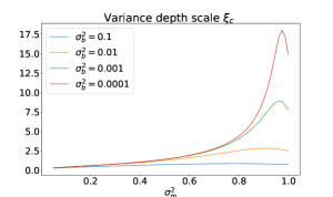
Refer to caption
Refer to caption
Figure 4: Depth scales as σm2superscriptsubscript𝜎𝑚2\sigma_{m}^{2} is varied. (a) The depth scale controlling the variance propagation of a signal (b) The depth scale controlling correlation propagation of two signals. Notice that the correlation depth scale ξcsubscript𝜉𝑐\xi_{c} only diverges as σm21superscriptsubscript𝜎𝑚21\sigma_{m}^{2}\to 1, whereas for standard continuous networks, there are an infinite number of such points, corresponding to various combinations of the weight and bias variances.

D.3 Jacobian mean squared singular value and Mean Field Gradient Backpropagation

An alternative perspective on critical initialisation, to be contrasted with the forward signal propagation theory, is that we are simply attempting to control the mean squared singular value of the input-output Jacobain matrix of the entire network, which we can decompose into the product of single layer Jacobian matrices. In standard networks, the single layer Jacobian mean squared singular value is equal to the derivative of the correlation mapping χ𝜒\chi as established in Poole et al. (2016). For the Gaussian model studied here this is not true, and corrections must be made to calculate the true mean squared singular value. This can be seen by observing the terms arising from denominator of the pre-activation field,

Jijsubscriptsuperscript𝐽𝑖𝑗\displaystyle J^{\ell}_{ij} =hi,ahj,a1=hj(h¯i,aΣii)=ϕ(hi,a)[MijΣii+(Mij)2h¯i,a(Σii)3/2ϕ(hi,a)]absentsubscriptsuperscript𝑖𝑎subscriptsuperscript1𝑗𝑎superscriptsubscript𝑗subscriptsuperscript¯𝑖𝑎subscriptsuperscriptΣ𝑖𝑖superscriptitalic-ϕsubscriptsuperscript𝑖𝑎delimited-[]superscriptsubscript𝑀𝑖𝑗subscriptsuperscriptΣ𝑖𝑖superscriptsuperscriptsubscript𝑀𝑖𝑗2subscriptsuperscript¯𝑖𝑎superscriptsubscriptsuperscriptΣ𝑖𝑖32italic-ϕsubscriptsuperscript𝑖𝑎\displaystyle=\frac{\partial h^{\ell}_{i,a}}{\partial h^{\ell-1}_{j,a}}=\frac{\partial}{\partial h_{j}^{\ell}}\bigg{(}\frac{\bar{h}^{\ell}_{i,a}}{\sqrt{\Sigma^{\ell}_{ii}}}\bigg{)}=\phi^{\prime}(h^{\ell}_{i,a})\big{[}\frac{M_{ij}^{\ell}}{\sqrt{\Sigma^{\ell}_{ii}}}+(M_{ij}^{\ell})^{2}\frac{\bar{h}^{\ell}_{i,a}}{(\Sigma^{\ell}_{ii})^{3/2}}\phi(h^{\ell}_{i,a})\big{]} (68)

Since ΣiisubscriptΣ𝑖𝑖\Sigma_{ii} is a quantity that scales with the layer width Nsubscript𝑁N_{\ell}, it is clear that when we consider squared quantities, such as the mean squared singular value, the second term, from the derivative of the denominator, will vanish in the large layer width limit. Thus the mean squared singular value of the single layer Jacobian approaches χ𝜒\chi. We will proceed as if χ𝜒\chi is the exact quantity we are interested in controlling.The analysis involved in determining whether the mean squared singular value is well approximated by χ𝜒\chi essentially takes us through the mean field gradient backpropagation theory as described in Schoenholz et al. (2016). This idea provides complementary depth scales for gradient signals travelling backwards.

Appendix E Reparameterisation trick surrogate

E.1 Signal propagation equations

We present, in slightly more detail, the signal propagation equations for the case of continuous neurons and stochastic binary weights yields the variance map,

qaa=𝔼ϕ2(hj,al1)+σb2subscript𝑞𝑎𝑎𝔼superscriptitalic-ϕ2superscriptsubscript𝑗𝑎𝑙1superscriptsubscript𝜎𝑏2\displaystyle q_{aa}=\mathbb{E}\phi^{2}(h_{j,a}^{l-1})+\sigma_{b}^{2} (69)

Thus, once again, the variance map does not depend on the variance of the means of the binary weights. The covariance map however does retain a dependence on σm2superscriptsubscript𝜎𝑚2\sigma_{m}^{2},

qablsuperscriptsubscript𝑞𝑎𝑏𝑙\displaystyle q_{ab}^{l} =σm2𝔼ϕ(hj,al1)ϕ(hj,al1)+σb2absentsuperscriptsubscript𝜎𝑚2𝔼italic-ϕsuperscriptsubscript𝑗𝑎𝑙1italic-ϕsuperscriptsubscript𝑗𝑎𝑙1superscriptsubscript𝜎𝑏2\displaystyle=\sigma_{m}^{2}\mathbb{E}\phi(h_{j,a}^{l-1})\phi(h_{j,a}^{l-1})+\sigma_{b}^{2} (70)

with the same expression as before. The correlation map is given by

cablsuperscriptsubscript𝑐𝑎𝑏𝑙\displaystyle c_{ab}^{l} =σm2𝔼ϕ(hj,al1)ϕ(hj,al1)+σb2𝔼ϕ2(hj,al1)+σb2absentsuperscriptsubscript𝜎𝑚2𝔼italic-ϕsuperscriptsubscript𝑗𝑎𝑙1italic-ϕsuperscriptsubscript𝑗𝑎𝑙1superscriptsubscript𝜎𝑏2𝔼superscriptitalic-ϕ2superscriptsubscript𝑗𝑎𝑙1superscriptsubscript𝜎𝑏2\displaystyle=\frac{\sigma_{m}^{2}\mathbb{E}\phi(h_{j,a}^{l-1})\phi(h_{j,a}^{l-1})+\sigma_{b}^{2}}{\mathbb{E}\phi^{2}(h_{j,a}^{l-1})+\sigma_{b}^{2}} (71)

and we have the derivative of the correlation map given by

χ𝜒\displaystyle\chi =σm2𝔼ϕ(hj,al1)ϕ(hj,bl1)absentsuperscriptsubscript𝜎𝑚2𝔼superscriptitalic-ϕsuperscriptsubscript𝑗𝑎𝑙1superscriptitalic-ϕsuperscriptsubscript𝑗𝑏𝑙1\displaystyle=\sigma_{m}^{2}\mathbb{E}\phi^{\prime}(h_{j,a}^{l-1})\phi^{\prime}(h_{j,b}^{l-1}) (72)

E.2 Determining the critical initialisation conditions

We recount the argument from the paper here. Since the mean variance σm2superscriptsubscript𝜎𝑚2\sigma_{m}^{2} does not appear in the variance map, we must once again consider different conditions for critical initialisation. Specifically, from the correlation map we have a fixed point c=1superscript𝑐1c^{*}=1 if and only if

σm2=1superscriptsubscript𝜎𝑚21\displaystyle\sigma_{m}^{2}=1 (73)

In turn, the condition χ1=1subscript𝜒11\chi_{1}=1 holds if

𝔼[(ϕ(hj,al1))2]=1σm2=1𝔼delimited-[]superscriptsuperscriptitalic-ϕsuperscriptsubscript𝑗𝑎𝑙121superscriptsubscript𝜎𝑚21\displaystyle\mathbb{E}[(\phi\ \!^{\prime}(h_{j,a}^{l-1}))^{2}]=\frac{1}{\sigma_{m}^{2}}=1 (74)

Thus, to find the critical initialisation, we need to find a value of qaa=𝔼ϕ2(hj,al1)+σb2subscript𝑞𝑎𝑎𝔼superscriptitalic-ϕ2superscriptsubscript𝑗𝑎𝑙1superscriptsubscript𝜎𝑏2q_{aa}=\mathbb{E}\phi^{2}(h_{j,a}^{l-1})+\sigma_{b}^{2} that satisfies this final condition. In the case that ϕ()=tanh()italic-ϕ\phi(\cdot)=\tanh(\cdot), then the function (ϕ(hj,al1))21superscriptsuperscriptitalic-ϕsuperscriptsubscript𝑗𝑎𝑙121(\phi\ \!^{\prime}(h_{j,a}^{l-1}))^{2}\leq 1, taking the value 111 at the origin only, this requires qaa0subscript𝑞𝑎𝑎0q_{aa}\to 0. Thus the critical initialisation is the singleton point (σb2,σm2)=(0,1)superscriptsubscript𝜎𝑏2superscriptsubscript𝜎𝑚201(\sigma_{b}^{2},\sigma_{m}^{2})=(0,1). This is confirmed by experiment, as we reported in the paper.

It is of course possible to investigate this perturbed surrogate for different noise models. For example, given different noise scaling κ𝜅\kappa, as in the previous chapter, there will be a corresponding σb2superscriptsubscript𝜎𝑏2\sigma_{b}^{2} that satisfy the critical initialisation condition. We leave such an investigation to future work, given the case of binary weights and continuous neurons does not appear to be of a particular interest over the binary neuron case.

Appendix F Signal propagation of binary networks

F.1 Forward signal propagation

In this neural network, it should be understood that all neurons are simply sign()sign\operatorname{sign}(\cdot) functions of their input, and all weights Wij{±1}superscriptsubscript𝑊𝑖𝑗plus-or-minus1W_{ij}^{\ell}\in\{\pm 1\} are randomly distributed according to

P(Wij=+1)=0.5𝑃superscriptsubscript𝑊𝑖𝑗10.5\displaystyle P(W_{ij}^{\ell}=+1)=0.5 (75)

thus maintaining a zero mean.

The pre-activation field is given by

hisuperscriptsubscript𝑖\displaystyle h_{i}^{\ell} =1N1jWijsign(hj1)+biabsent1subscript𝑁1subscript𝑗superscriptsubscript𝑊𝑖𝑗signsuperscriptsubscript𝑗1superscriptsubscript𝑏𝑖\displaystyle=\frac{1}{\sqrt{N_{\ell-1}}}\sum_{j}W_{ij}^{\ell}\operatorname{sign}(h_{j}^{\ell-1})+b_{i}^{\ell} (77)

So, the length map is:

qaasuperscriptsubscript𝑞𝑎𝑎\displaystyle q_{aa}^{\ell} =Dz(sign(qaa1z)2)+σb2\displaystyle=\int Dz(\operatorname{sign}(\sqrt{q_{aa}^{\ell-1}}z)^{2})+\sigma_{b}^{2} (78)
=1+σb2absent1superscriptsubscript𝜎𝑏2\displaystyle=1+\sigma_{b}^{2} (79)

Interestingly, this is the same value as for the perturbed Gaussian with stochastic binary weights and neurons.

The covariance evolves as

qabsuperscriptsubscript𝑞𝑎𝑏\displaystyle q_{ab}^{\ell} =Dz1Dz2sign(ua)sign(ub)+σb2absent𝐷subscript𝑧1𝐷subscript𝑧2signsubscript𝑢𝑎signsubscript𝑢𝑏superscriptsubscript𝜎𝑏2\displaystyle=\int Dz_{1}Dz_{2}\operatorname{sign}(u_{a})\operatorname{sign}(u_{b})+\sigma_{b}^{2} (80)

we again have a correlation map:

cab=Dz1Dz2sign(ua)sign(ub)+σb2qaa1qbb1subscriptsuperscript𝑐𝑎𝑏𝐷subscript𝑧1𝐷subscript𝑧2signsubscript𝑢𝑎signsubscript𝑢𝑏superscriptsubscript𝜎𝑏2subscriptsuperscript𝑞1𝑎𝑎subscriptsuperscript𝑞1𝑏𝑏\displaystyle c^{\ell}_{ab}=\frac{\int Dz_{1}Dz_{2}\operatorname{sign}(u_{a})\operatorname{sign}(u_{b})+\sigma_{b}^{2}}{\sqrt{q^{\ell-1}_{aa}q^{\ell-1}_{bb}}} (81)

where as in the paper, ua=qaa1z1,ub=qbb1(cab1z1+1(cab1)2z2)formulae-sequencesubscript𝑢𝑎superscriptsubscript𝑞𝑎𝑎1subscript𝑧1subscript𝑢𝑏superscriptsubscript𝑞𝑏𝑏1superscriptsubscript𝑐𝑎𝑏1subscript𝑧11superscriptsuperscriptsubscript𝑐𝑎𝑏12subscript𝑧2u_{a}\!=\sqrt{q_{aa}^{\ell-1}}z_{1},\ u_{b}\!=\sqrt{q_{bb}^{\ell-1}}\big{(}c_{ab}^{\ell-1}z_{1}+\sqrt{1-(c_{ab}^{\ell-1})^{2}}z_{2}\big{)}.

We can find this correlation in closed form. First we rewrite our integral with hh, for a joint density p(ha,hb)𝑝subscript𝑎subscript𝑏p(h_{a},h_{b}), and then rescale the hasubscript𝑎h_{a} such that the variance is 1, so that dha=qaadva𝑑subscript𝑎subscript𝑞𝑎𝑎𝑑subscript𝑣𝑎dh_{a}=\sqrt{q_{aa}}dv_{a}

𝑑ha𝑑hbsign(ha)sign(hb)p(ha,hb)differential-dsubscript𝑎differential-dsubscript𝑏signsubscript𝑎signsubscript𝑏𝑝subscript𝑎subscript𝑏\displaystyle\int dh_{a}dh_{b}\operatorname{sign}(h_{a})\operatorname{sign}(h_{b})p(h_{a},h_{b}) =𝑑va𝑑vbsign(va)sign(vb)p(va,vb)absentdifferential-dsubscript𝑣𝑎differential-dsubscript𝑣𝑏signsubscript𝑣𝑎signsubscript𝑣𝑏𝑝subscript𝑣𝑎subscript𝑣𝑏\displaystyle=\int dv_{a}dv_{b}\operatorname{sign}(v_{a})\operatorname{sign}(v_{b})p(v_{a},v_{b}) (82)
=(2P(v1>0,v2>0)2P(v1>0,v2<0))absent2𝑃formulae-sequencesubscript𝑣10subscript𝑣202𝑃formulae-sequencesubscript𝑣10subscript𝑣20\displaystyle=\big{(}2P(v_{1}>0,v_{2}>0)-2P(v_{1}>0,v_{2}<0)\big{)} (83)

where p(va,vb)𝑝subscript𝑣𝑎subscript𝑣𝑏p(v_{a},v_{b}) is a joint with the same correlation cabsubscript𝑐𝑎𝑏c_{ab} (which is now equal to its covariance), and the capital P(v1,v2)𝑃subscript𝑣1subscript𝑣2P(v_{1},v_{2}) corresponds to the (cumulative) distribution function. A standard result for standard bivariate normal distributions with correlation ρ𝜌\rho,

P(v1>0,v2>0)=14+sin1(ρ)2π,P(v1>0,v2<0)=cos1(ρ)2πformulae-sequence𝑃formulae-sequencesubscript𝑣10subscript𝑣2014superscript1𝜌2𝜋𝑃formulae-sequencesubscript𝑣10subscript𝑣20superscript1𝜌2𝜋\displaystyle P(v_{1}>0,v_{2}>0)=\frac{1}{4}+\frac{\sin^{-1}(\rho)}{2\pi},\qquad P(v_{1}>0,v_{2}<0)=\frac{\cos^{-1}(\rho)}{2\pi} (84)

So we then have that

𝑑ha𝑑hbϕ(ha)ϕ(hb)p(ha,hb)differential-dsubscript𝑎differential-dsubscript𝑏italic-ϕsubscript𝑎italic-ϕsubscript𝑏𝑝subscript𝑎subscript𝑏\displaystyle\int dh_{a}dh_{b}\phi(h_{a})\phi(h_{b})p(h_{a},h_{b}) =qaaqbb(12+sin1(cab1)πcos1(cab1)π)absentsubscript𝑞𝑎𝑎subscript𝑞𝑏𝑏12superscript1subscriptsuperscript𝑐1𝑎𝑏𝜋superscript1subscriptsuperscript𝑐1𝑎𝑏𝜋\displaystyle=\sqrt{q_{aa}q_{bb}}\big{(}\frac{1}{2}+\frac{\sin^{-1}(c^{\ell-1}_{ab})}{\pi}-\frac{\cos^{-1}(c^{\ell-1}_{ab})}{\pi}\big{)} (85)

Thus the correlation map is:

cabsubscriptsuperscript𝑐𝑎𝑏\displaystyle c^{\ell}_{ab} =(12+sin1(cab1)πcos1(cab1)π)+σb2qaa1qbb1absent12superscript1subscriptsuperscript𝑐1𝑎𝑏𝜋superscript1subscriptsuperscript𝑐1𝑎𝑏𝜋superscriptsubscript𝜎𝑏2subscriptsuperscript𝑞1𝑎𝑎subscriptsuperscript𝑞1𝑏𝑏\displaystyle=\frac{\big{(}\frac{1}{2}+\frac{\sin^{-1}(c^{\ell-1}_{ab})}{\pi}-\frac{\cos^{-1}(c^{\ell-1}_{ab})}{\pi}\big{)}+\sigma_{b}^{2}}{\sqrt{q^{\ell-1}_{aa}q^{\ell-1}_{bb}}} (86)
=2πsin1(cab1)+σb2qaa1qbb1absent2𝜋superscript1subscriptsuperscript𝑐1𝑎𝑏superscriptsubscript𝜎𝑏2subscriptsuperscript𝑞1𝑎𝑎subscriptsuperscript𝑞1𝑏𝑏\displaystyle=\frac{\frac{2}{\pi}\sin^{-1}(c^{\ell-1}_{ab})+\sigma_{b}^{2}}{\sqrt{q^{\ell-1}_{aa}q^{\ell-1}_{bb}}} (87)

Since, from before we have qaa=1+σb2subscript𝑞𝑎𝑎1superscriptsubscript𝜎𝑏2q_{aa}=1+\sigma_{b}^{2}, we then obtain

cabsubscriptsuperscript𝑐𝑎𝑏\displaystyle c^{\ell}_{ab} =2πsin1(cab1)+σb21+σb2absent2𝜋superscript1subscriptsuperscript𝑐1𝑎𝑏superscriptsubscript𝜎𝑏21superscriptsubscript𝜎𝑏2\displaystyle=\frac{\frac{2}{\pi}\sin^{-1}(c^{\ell-1}_{ab})+\sigma_{b}^{2}}{1+\sigma_{b}^{2}} (88)

Recall that sin1(1)=π2superscript11𝜋2\sin^{-1}(1)=\frac{\pi}{2}, so we have that c=1superscript𝑐1c^{*}=1 is a fixed point always.

We will now derive its slope, denoted as χ=cabcab1𝜒subscriptsuperscript𝑐𝑎𝑏subscriptsuperscript𝑐1𝑎𝑏\chi=\frac{\partial c^{\ell}_{ab}}{\partial c^{\ell-1}_{ab}}, but by first integrating over the ϕ()=sign()italic-ϕsign\phi()=\operatorname{sign}() non-linearities, and then taking the derivative.

Now we are in a place to take the derivative :

χ=cabcab1=2π1qaa1qbb111(cab1)2=2π1(1+σb2)11(cab1)2𝜒subscriptsuperscript𝑐𝑎𝑏subscriptsuperscript𝑐1𝑎𝑏2𝜋1subscriptsuperscript𝑞1𝑎𝑎subscriptsuperscript𝑞1𝑏𝑏11superscriptsubscriptsuperscript𝑐1𝑎𝑏22𝜋11superscriptsubscript𝜎𝑏211superscriptsubscriptsuperscript𝑐1𝑎𝑏2\displaystyle\chi=\frac{\partial c^{\ell}_{ab}}{\partial c^{\ell-1}_{ab}}=\frac{2}{\pi}\frac{1}{\sqrt{q^{\ell-1}_{aa}q^{\ell-1}_{bb}}}\frac{1}{\sqrt{1-(c^{\ell-1}_{ab})^{2}}}=\frac{2}{\pi}\frac{1}{(1+\sigma_{b}^{2})}\frac{1}{\sqrt{1-(c^{\ell-1}_{ab})^{2}}} (89)

We can see that the derivative χ𝜒\chi diverges at cab=1subscriptsuperscript𝑐𝑎𝑏1c^{\ell}_{ab}=1, meaning that there is no critical initialisation for this system. This of course means that correlations will not propagate to arbitrary depth in deterministic binary networks, as one might have expected.

F.2 Stochastic weights and neurons

We begin again with the variance map,

qaalsuperscriptsubscript𝑞𝑎𝑎𝑙\displaystyle q_{aa}^{l} =𝔼[(hi,al)2]absent𝔼delimited-[]superscriptsuperscriptsubscript𝑖𝑎𝑙2\displaystyle=\mathbb{E}\left[(h_{i,a}^{l})^{2}\right] (90)

where in this the field is given by

hi,alsuperscriptsubscript𝑖𝑎𝑙\displaystyle h_{i,a}^{l} =1NjWijlxhj,al1+bilabsent1𝑁subscript𝑗superscriptsubscript𝑊𝑖𝑗𝑙subscript𝑥superscriptsubscript𝑗𝑎𝑙1superscriptsubscript𝑏𝑖𝑙\displaystyle=\frac{1}{\sqrt{N}}\sum_{j}W_{ij}^{l}x_{h_{j,a}^{l-1}}+b_{i}^{l} (91)

where xhj,al1subscript𝑥superscriptsubscript𝑗𝑎𝑙1x_{h_{j,a}^{l-1}} denotes a stochastic binary neuron whose natural parameter is the pre-activation from the previous layer.

The expectation for the length map is defined in terms of nested conditional expectations, since we wish to average over all random elements in the forward pass,

qaasuperscriptsubscript𝑞𝑎𝑎\displaystyle q_{aa}^{\ell} =𝔼h𝔼x|hxhj,al1+σb2absentsubscript𝔼subscript𝔼conditional𝑥subscript𝑥superscriptsubscript𝑗𝑎𝑙1superscriptsubscript𝜎𝑏2\displaystyle=\mathbb{E}_{h}\mathbb{E}_{x|h}x_{h_{j,a}^{l-1}}+\sigma_{b}^{2} (92)
=1+σb2absent1superscriptsubscript𝜎𝑏2\displaystyle=1+\sigma_{b}^{2} (93)

Once again, this is the same value as for the perturbed Gaussian with stochastic binary weights and neurons.

Similarly, the covariance map gives us,

qablsuperscriptsubscript𝑞𝑎𝑏𝑙\displaystyle q_{ab}^{l} =𝔼[hi,alhi,bl]absent𝔼delimited-[]superscriptsubscript𝑖𝑎𝑙superscriptsubscript𝑖𝑏𝑙\displaystyle=\mathbb{E}\left[h_{i,a}^{l}h_{i,b}^{l}\right] (94)
=𝔼ha,hb𝔼xb|ha𝔼xb|hbxhj,al1xhj,bl1+σb2absentsubscript𝔼subscript𝑎subscript𝑏subscript𝔼conditionalsubscript𝑥𝑏subscript𝑎subscript𝔼conditionalsubscript𝑥𝑏subscript𝑏subscript𝑥superscriptsubscript𝑗𝑎𝑙1subscript𝑥superscriptsubscript𝑗𝑏𝑙1superscriptsubscript𝜎𝑏2\displaystyle=\mathbb{E}_{h_{a},h_{b}}\mathbb{E}_{x_{b}|h_{a}}\mathbb{E}_{x_{b}|h_{b}}x_{h_{j,a}^{l-1}}x_{h_{j,b}^{l-1}}+\sigma_{b}^{2} =𝔼ϕ(hj,al1)ϕ(hj,al1)+σb2absent𝔼italic-ϕsuperscriptsubscript𝑗𝑎𝑙1italic-ϕsuperscriptsubscript𝑗𝑎𝑙1superscriptsubscript𝜎𝑏2\displaystyle=\mathbb{E}\phi(h_{j,a}^{l-1})\phi(h_{j,a}^{l-1})+\sigma_{b}^{2} (95)

with phi()𝑝𝑖phi(\cdot) being the mean function, or a shifted and scaled version of the cumulative distribution function for the stochastic binary neurons, just as in previous Chapters. This expression is equivalent to the perturbed surrogate for stochastic binary weights and neurons, with a mean variance of σm2=1superscriptsubscript𝜎𝑚21\sigma_{m}^{2}=1. Following the arguments for that surrogate, no critical initialisation exists.

F.3 Stochastic binary weights and continuous neurons

In this case, as we show in the appendix, the resulting equations are

qaasuperscriptsubscript𝑞𝑎𝑎\displaystyle q_{aa}^{\ell} =𝔼ϕ2(hj,al1)+σb2absent𝔼superscriptitalic-ϕ2superscriptsubscript𝑗𝑎𝑙1superscriptsubscript𝜎𝑏2\displaystyle=\mathbb{E}\phi^{2}(h_{j,a}^{l-1})+\sigma_{b}^{2} (96)
qablsuperscriptsubscript𝑞𝑎𝑏𝑙\displaystyle q_{ab}^{l} =𝔼ϕ(hj,al1)ϕ(hj,al1)+σb2absent𝔼italic-ϕsuperscriptsubscript𝑗𝑎𝑙1italic-ϕsuperscriptsubscript𝑗𝑎𝑙1superscriptsubscript𝜎𝑏2\displaystyle=\mathbb{E}\phi(h_{j,a}^{l-1})\phi(h_{j,a}^{l-1})+\sigma_{b}^{2} (97)

which are, once again, the same as for the perturbed surrogate in this case, with σm2=1superscriptsubscript𝜎𝑚21\sigma_{m}^{2}=1. This means that this model does have a critical initialisation, at the point (σm2,σb2)=(1,0)superscriptsubscript𝜎𝑚2superscriptsubscript𝜎𝑏210(\sigma_{m}^{2},\sigma_{b}^{2})=(1,0).

F.4 Continuous weights and stochastic binary neurons

Similar arguments to the above show that the equations for this case are exactly equivalent to the perturbed surrogate model. This means that no critical initialisation exists in this case either.

Appendix G Miscellaneous comments

G.1 Remark: Valdity of the CLT for the first level of mean field

A legitimate immediate concern with initialisations that send σm21superscriptsubscript𝜎𝑚21\sigma_{m}^{2}\to 1 may be that the binary stochastic weights 𝐒ijsuperscriptsubscript𝐒𝑖𝑗{\bf S}_{ij}^{\ell} are no longer stochastic, and that the variance of the Gaussian under the central limit theorem would no longer be correct. First recall the CLT’s variance is given by Var(𝐡)=j(1mj2xj2)Varsuperscript𝐡subscript𝑗1superscriptsubscript𝑚𝑗2superscriptsubscript𝑥𝑗2\text{Var}({\bf h}^{\ell})=\sum_{j}(1-m_{j}^{2}x_{j}^{2}). If the means mj±1subscript𝑚𝑗plus-or-minus1m_{j}\to\pm 1 then variance is equal in value to jmj2(1xj2)subscript𝑗superscriptsubscript𝑚𝑗21superscriptsubscript𝑥𝑗2\sum_{j}m_{j}^{2}(1-x_{j}^{2}), which is the central limit variance in the case of only stochastic binary neurons at initialisation. Therefore, the applicability of the CLT is invariant to the stochasticity of the weights. This is not so of course if both neurons and weights are deterministic, for example if neurons are just tanh()\tanh() functions.