Log surfaces of Picard rank one
from four lines in the plane

Abstract.

We derive simple formulas for the basic numerical invariants of a singular surface with Picard number one obtained by blowups and contractions of the four-line configuration in the plane. As an application, we establish the smallest positive volume and the smallest accumulation point of volumes of log canonical surfaces obtained in this way.

1. Introduction

Let $X$ be a projective normal surface and $B=\sum b_{i}B_{i}$ be an ${\mathbb{R}}$-divisor with coefficients in a DCC set, i.e. one satisfying the descending chain condition. Assume that the pair $(X,B)$ has log canonical singularities and that the log canonical divisor $K_{X}+B$ is ample. It is known from [Ale94] that the set of volumes $(K_{X}+B)^{2}$ is also a DCC set and thus attains the absolute minimum, a positive real number. The paper [AM04] gives an effective lower bound for it which however is unrealistically small.

In [AL16] we found surfaces with the smallest known volumes for the sets ${\mathcal{S}}_{0}=\{0\}$ and ${\mathcal{S}}_{1}=\{0,1\}$. In [AL18] we proved reasonable lower bounds for the accumulation points of the sets of these volumes. All of the best known examples (including for other common DCC sets ${\mathcal{S}}$) are based on the following construction which despite its simplicity is expected to be optimal.

Construction 1.1.

Let $L_{1},L_{2},L_{3},L_{4}$ be four lines in general position in the projective plane. Consider a diagram

in which $f\colon Y\to{\mathbb{P}}^{2}$ is a sequence of blowups at the points of intersection between the curves which are either strict preimages of $L_{k}$ or are exceptional divisors $E_{j}$. We will call these curves the visible curves. The morphism $g\colon Y\to X$ is a contraction of some of the visible curves to a normal surface $X$. The images $B_{i}$ of the non-contracted visible curves are called survivors. We will consider pairs $(X,B)$, where $B=\sum b_{i}B_{i}$ is a linear combination of survivors.

In this paper we tackle the case when the Picard number $\rho(X)$ is 1, i.e. when there are exactly 4 survivors. In this case the record surface in [AL16] for the sets ${\mathcal{S}}_{0}$ and ${\mathcal{S}}_{1}$ has volume $\frac{1}{6351}$. Here we prove that this bound is optimal for the sets ${\mathcal{S}}_{0},{\mathcal{S}}_{1}$ and Picard number 1, for the surfaces in Construction 1.1. We also prove that the minimum of the limit points of these volumes is $\frac{1}{78}$. (Note however that the absolute champions in [AL16] have $\rho=2$.)

The main contribution of this paper is a simple explicit formula for $(K_{X}+B)^{2}$ which we then apply. This formula works without assuming that $K_{X}+B$ is ample or that $(X,B)$ has log canonical singularities, and may be used in other situations, for example for log del Pezzo and log Calabi-Yau (or Enriques) surfaces.

Dongseon Hwang has informed us that he ran some computer experiments for surfaces of Picard number 1 that did not yield a volume better than $\frac{1}{6351}$ found in [AL16]. Actually proving this bound, for example in the way we did it in [AL16, Thm. 8.2] for a special case, was the main motivation for this paper.

2. Surface singularities and their determinants

Let $X$ be a normal surface and $B=\sum b_{i}B_{i}$ be a ${\mathbb{Q}}$- or ${\mathbb{R}}$-divisor with coefficients $0\leq b_{i}\leq 1$. Let $f\colon Y\to X$ be a resolution of singularities with a normal crossing divisor $f_{*}^{-1}B\cup\operatorname{Exc}(\pi)$. Consider the natural formula

$$K_{Y}=f^{*}(K_{X}+B)+\sum a_{j}E_{j}.$$

Here, the divisors $E_{j}$ are both the $f$-exceptional divisors and the strict preimages of the divisors $B_{i}$; for the latter one has $a_{i}=-b_{i}$. The numbers $a_{j}$ are called discrepancies, $c_{j}=1+a_{j}$ are log discrepancies, and $b_{j}=-a_{j}=1-c_{j}$ are codiscrepancies. The pair $(X,B)$ is called log canonical or lc (resp. Kawamata log terminal or klt) if all $a_{j}\geq-1$, i.e. $c_{j}\geq 0$ (resp. $a_{j}>-1$, $c_{j}>0$, $b_{j}<1$). One says that $(X,B)$ is canonical at a point $p\in X$ if the discrepancy for any exceptional divisor over $p$ is nonnegative.

Log canonical singularities of surfaces in any characteristic are classified by their dual graphs, cf. [Ale92]. When $B=0$ the answer is as follows.

Definition 2.1.

Let $f\colon{\widetilde{X}}\to(X,0)$ be the minimal resolution and $E_{i}$ be the $f$-exceptional divisors. The dual graph has a vertex for each curve $E_{i}$, marked by a positive integer $n_{i}=-E_{i}^{2}$. Two vertices are connected by $E_{i}.E_{j}$ edges. Vice versa, each marked multigraph gives a quadratic form $(-E_{i}.E_{j})$. For simplicity we always work with the negative of the intersection matrix since it is positive definite. The diagonal entries of such a matrix are $>0$ and the off-diagonal entries are $\leq 0$.

Then, first of all, singularities corresponding to arbitrary chains $[n_{1},\dotsc,n_{k}]$ with $n_{i}\geq 2$ are klt. These are in a bijection with rational numbers $0<\frac{p}{q}<1$ via the Hirzebruch-Jung (HJ) continued fractions

$$\frac{q}{p}=n_{1}-\frac{1}{n_{2}-\frac{1}{n_{3}-\dots}}.$$

Here, $q=\det(-E_{i}.E_{j})$ is the determinant of the matrix with the diagonal entries $n_{i}$ and with $-1$ on the diagonals adjacent to it. Our notation for this determinant is $|n_{1},n_{2},\dotsc,n_{k}|$.

Remark 2.2.

We will need a slight generalization of this constructions, as follows. Let $\frac{p}{q}$ be a fraction larger than or equal to 1, so that $\frac{q}{p}\leq 1$. Then by the same continued fraction expansion it corresponds to the chain $[1,n_{2},\dotsc,n_{k}]$. In this way, we get a bijection between the positive rational numbers $\frac{p}{q}$ and the chains $[n_{1},n_{2},\dotsc,n_{k}]$ in which the starting number is $n_{1}\geq 1$ and all others are $n_{i}\geq 2$.

In addition to the chains, graphs with a positive definite quadratic form and a single fork from which three chains with determinants $q_{1},q_{2},q_{3}$ emanate are klt iff $\frac{1}{q_{1}}+\frac{1}{q_{2}}+\frac{1}{q_{3}}>1$, and they are log canonical iff $\frac{1}{q_{1}}+\frac{1}{q_{2}}+\frac{1}{q_{3}}\geq 1$. The possibilities for $(q_{1},q_{2},q_{3})$ are $(2,2,n)$, $(2,3,3)$, $(2,3,4)$, $(2,3,5)$, $(3,3,3)$, $(2,4,4)$, $(2,3,6)$ and correspond to the Lie types $D_{n+2}$, $E_{6}$, $E_{7}$, $E_{8}$, ${\widetilde{E}}_{6}$, ${\widetilde{E}}_{7}$, ${\widetilde{E}}_{8}$. There is also a graph of type ${\widetilde{D}}_{n}$ with two forks and four legs with determinants $(2,2,2,2)$. Finally, there is graph of type ${\widetilde{A}}_{n}$ which is a cycle. For the ${\widetilde{A}}_{1}$ and ${\widetilde{A}}_{2}$ graphs, the curves $E_{i}$ should intersect at distinct point: tacnode and triple points are not allowed. We denote the determinant of the cycle with marks $n_{i}$ by $|n_{1},n_{2},\dotsc,n_{k},\circlearrowleft|$.

Remark 2.3.

When all the marks are $n_{i}=2$, the above are the dual graphs of Du Val singularities and of Kodaira’s degenerations of elliptic curves. But here any marks $n_{i}$ are allowed, as long as the form $(-E_{i}.E_{j})$ is positive definite.

For the set ${\mathcal{S}}_{1}=\{0,1\}$ and $B\neq 0$, i.e. when $B$ is nonempty and reduced, one can have $B$ to be attached to one or both ends of a chain, and to a leg of a $D_{n}$ graph if the other legs have $(q_{1},q_{2})=(2,2)$. A degenerate case of this is attaching $B$ to the middle of a chain $[2,n,2]$, this is also allowed. This completes the list.

Lemma 2.4.

Divide the set of vertices $V(\Gamma)$ into two disjoint subsets $V_{1}\sqcup V_{2}$, and let $\Gamma_{i}$ will be the induced subgraphs on these vertex sets. Assume that there are no cycles in $\Gamma$ involving both $\Gamma_{1}$ and $\Gamma_{2}$, in other words $h_{1}(\Gamma)=h_{1}(\Gamma_{1})+h_{1}(\Gamma_{2})$, where $h_{1}$ denotes the rank of the first homology group of a connected graph. Then

$$\det\Gamma=\det\Gamma_{1}\cdot\det\Gamma_{2}+(-1)^{k}\hskip-22.0pt\sum_{(u_{1},v_{1}),\dotsc,(u_{k},v_{k})}\hskip-22.0pt\det(\Gamma_{1}-u_{1}\dotsc-u_{k})\cdot\det(\Gamma_{2}-v_{1}\dotsc-v_{k}),$$

in which the sum goes over collections of edges $(u_{i},v_{i})$ in $\Gamma$ with $u_{i}\in\Gamma_{1}$, $v_{i}\in\Gamma_{2}$.

Proof.

In the expansion of $\det\Gamma$ into the sum of $n!$ products, the terms which are not listed in the above formula correspond to paths that enter from $\Gamma_{1}$ into $\Gamma_{2}$ and then eventually die, as there are no cycles coming back. ∎

Corollary 2.5.

One has $|n_{1},n_{2},\dotsc,n_{k}|=n_{1}\cdot|n_{2},\dotsc,n_{k}|-|n_{3}\dotsc,n_{k}|$ and
$|n_{1},\dotsc,n_{i},n_{i+1},\dotsc n_{k}|=|n_{1},\dotsc,n_{i}|\cdot|n_{i+1},\dotsc n_{k}|-|n_{1},\dotsc,n_{i-1}|\cdot|n_{i+2},\dotsc n_{k}|.$

Here, by convention, the determinant of a chain of length $k=0$ is 1. There is a generalization of (2.4) when there are cycles between $\Gamma_{1},\Gamma_{2}$. We will not need it since the only non-tree log canonical graph is a cycle. For it, it is easy to prove

$$|n_{1},n_{2},\dotsc,n_{k},\circlearrowleft|=n_{1}\cdot|n_{2},\dotsc,n_{k}|-|n_{3},\dotsc,n_{k}|-|n_{2},\dotsc,n_{k-1}|-2,$$

with 2 accounting for the two directed cycles in $\Gamma$, clockwise and counter clockwise.

Corollary 2.6.

The determinant of a graph $[(m-1)\times 2]\cup\Gamma$ obtained by attaching the chain $[(m-1)\times 2]=[2,\dotsc,2]$ of $(m-1)$ 2’s to a vertex $v$ with mark $n$ is

$$\det\,[(m-1)\times 2]\cup[n]\cup\Gamma^{\prime}=-\det\,[-m,n-1]\cup\Gamma^{\prime}.$$

where $\Gamma^{\prime}=\Gamma-v$ and $[-m,n-1]\cup\Gamma^{\prime}$ is the graph obtained by replacing the mark $n$ of $v\in\Gamma$ by $n-1$ and attaching a single vertex marked $-m$.

Proof.

Applying 2.4 twice gives

$$\det\,[(m-1)\times 2]\cup[n]\cup\Gamma^{\prime} = m\det\,[n]\cup\Gamma\ -\ (m-1)\det\,\Gamma^{\prime}\quad\text{and}$$

$$\det\,[-m,n-1]\cup\Gamma^{\prime} = (-m)\det\,[n-1]\cup\Gamma^{\prime}\ -\ \det\,\Gamma^{\prime}$$

$$= (-m)\det\,[n]\cup\Gamma^{\prime}+m\det\,\Gamma^{\prime}-\det\Gamma^{\prime}.$$

∎

Below, we will need to deal with the following situation. Let $\bm{\Gamma}(n_{i})$ be a “core graph” with the vertices marked $n_{i}$. On top of each vertex $v_{i}$ we “graft” several chains corresponding to HJ fractions $\frac{q_{ij}}{p_{ij}}$ as in Remark 2.2. We emphasize that we do not attach a chain. Instead, grafting means that we put an end of the chain for the fraction $\frac{q_{ij}}{p_{ij}}$ on top of the vertex $v_{i}$. Thus, if

$$\frac{p_{ij}}{q_{ij}}=n_{ij}-\frac{r_{ij}}{q_{ij}},\qquad p_{ij}=n_{ij}q_{ij}-r_{ij}$$

then the mark of the vertex $v_{i}$ in the new graph is $n_{i}+\sum_{j}n_{ij}$ and the legs have determinants $q_{ij}$. The legs “attached” to the core correspond to the fractions $\frac{r_{ij}}{q_{ij}}$.

We will call thus obtained graph $\widehat{\Gamma}\big{(}n_{i};\frac{q_{ij}}{p_{ij}}\big{)}$ a “hairy graph”, with hairs being the chains coming out of the vertices of the core graph.

Theorem 2.7.

The determinant of a hairy graph can be computed by the formula

$$\det\widehat{\Gamma}\big{(}n_{i};\frac{q_{ij}}{p_{ij}}\big{)}=\det\bm{\Gamma}\big{(}n_{i}+\sum_{j}\frac{p_{ij}}{q_{ij}}\big{)}\cdot\prod_{i,j}q_{ij}$$

where the core graph $\bm{\Gamma(n_{i})}$ has new marks $\bm{n_{i}}=n_{i}+\sum_{j}\frac{p_{ij}}{q_{ij}}$. Alternatively,

$$\det\widehat{\Gamma}\big{(}n_{i};\frac{q_{ij}}{p_{ij}}\big{)}=\det\bm{\widetilde{\Gamma}}\big{(}n_{i};-\frac{q_{ij}}{p_{ij}}\big{)}\cdot\prod_{i,j}(-p_{ij})$$

where the graph $\bm{\widetilde{\Gamma}}$ is obtained from the graph $\Gamma(n_{i})$ by adding a single vertex of weight $-\frac{q_{ij}}{p_{ij}}$ for each hair.

Proof.

Follows by repeatedly applying Lemma 2.4. ∎

Example 2.8.

Attaching the chain $[(m-1)\times 2]$ to a vertex with mark $n$ is the same as grafting the chain $[1,(m-1)\times 2]$ onto a vertex with mark $(n-1)$. The chain $[1,(m-1)\times 2]$ corresponds to the HJ fraction $\frac{q}{p}=\frac{m}{1}$. The second formula of (2.7) is now precisely (2.6). The first formula of (2.7) gives an alternative expression for this determinant as $m\det\bm{\Gamma}$, where $\bm{\Gamma}$ is the core graph with the weight ${\bm{n}}=n-1+\frac{1}{m}$ at the vertex $v$.

3. Weight vectors of visible curves and weight matrices

We follow the notations of Construction 1.1. Here, we encode each visible curve uniquely by a weight vector in ${\mathbb{Z}}^{4}$, and the entire surface $X$ by a weight matrix.

Definition 3.1.

The weight vector of a line $L_{i}$ is the vector $e_{i}$ in the standard Euclidean basis of ${\mathbb{Z}}^{4}$. For an exceptional curve $E$ of $f$ its weight vector is $(w_{1},w_{2},w_{3},w_{4})$, where $w_{i}$ is the coefficient of $E$ in the full pullback $f^{*}(L_{i})$.

In our situation, every visible curve other than $f_{*}^{-1}L_{i}$ lies over the intersection of exactly two lines, say $L_{i}\cap L_{j}$. For it, $w_{i}>0$, $w_{j}>0$ and $w_{k}=0$ for $k\neq i,j$. We can identify a weight vector with $w_{i}w_{j}\neq 0$ to an element in $\mathbb{Z}_{i}\times\mathbb{Z}_{j}\cong\mathbb{Z}^{2}$ where $\mathbb{Z}_{i}$ and $\mathbb{Z}_{j}$ are the $i$-th and $j$-th factors of $\mathbb{Z}^{4}$ respectively.

Definition 3.2.

The weight matrix $W$ of a surface $X$ is an $N\times 4$ matrix whose rows are the weight vectors of the survivors $E_{1},\dotsc,E_{N}$, where $N=\rho(X)+3$. Thus, the four columns of $W$ are the pullbacks $f^{*}(L_{i})$ for the four lines, written as linear combinations of the visible curves, with all but coefficients in $E_{i}$ ignored.

The reduced weight matrix ${\overline{W}}$ is an $N\times 3$ matrix with columns $f^{*}(L_{i}-L_{4})$.

Definition 3.3.

Given a pair $(X,B=\sum b_{i}B_{i})$ as in Construction 1.1, the extended weight matrix ${\widehat{W}}$ is an $(N+1)\times 5$ matrix whose entries in the last column are the log discrepancies $c_{i}=1-b_{i}$, and with the row $(1,\dotsc,1)$ added at the bottom.

Note that $W$ and ${\widehat{W}}$ are square matrices iff $\rho(X)=1$, of sizes $4\times 4$ and $5\times 5$ respectively. We now establish a description of the dual graph of the visible curves on $Y$ in terms of the weight vectors. We begin with the following situation.

Construction 3.4.

Let $L_{i},L_{j}$ be two smooth curves on a smooth surface $S$, intersecting normally at a single point $P$. These are not necessarily lines in ${\mathbb{P}}^{2}$; we will later apply this to the lines. Since there is only one point, the weight vector will be in ${\mathbb{Z}}^{2}$ and not ${\mathbb{Z}}^{4}$. We will begin with the initial dual graph that is the edge $\{v_{i},v_{j}\}$ and we will give the vertices the initial marks 0.

Now consider a sequence of blowups $Y\to S$ over $P$. Each blowup introduces a $(-1)$-curve $E$. On the next surface let us blow up one of the two points of intersection of $E$ with the neighboring visible curves, either the one on the left or the one on the right. The old $(-1)$-curve becomes a $(-2)$-curve and there is a new $(-1)$-curve. Then we repeat. Thus, the entire procedure is encoded in a binary sequence, such as LRRRLR. Let $(w_{i},w_{j})\in{\mathbb{Z}}^{2}$ be the weight vector of the $(-1)$-curve $E$ after the final blowup: $w_{i}$ is the coefficient of $E$ in $f^{*}L_{i}$ and $w_{j}$ is the coefficient of $E$ in $f^{*}L_{j}$. Let $\Gamma$ be the final graph; it is a chain.

Theorem 3.5.

In Construction 3.4, let $\Gamma_{i}$ be the chain on the left of the $(-1)$-curve $E$ in the final graph $\Gamma$, the one containing $v_{i}$. Let $\Gamma_{j}$ be the chain to the right of $E$, the one containing $v_{j}$. Then

1. $\det\Gamma_{i}=w_{i}$ and $\det(\Gamma_{i}-v_{i})=w_{j}$.

2. $\det\Gamma_{j}=w_{j}$ and $\det(\Gamma_{j}-v_{j})=w_{i}$.

In other words, $\Gamma_{i}$ corresponds to the HJ fraction $\frac{w_{j}}{w_{i}}$ and $\Gamma_{j}$ to $\frac{w_{i}}{w_{j}}$. In this way, all the possible visible curves on the blowups over the point $P$ are in a bijection with the pairs of coprime positive integers $(w_{i},w_{j})$, or equivalently with the positive rational numbers $\frac{w_{j}}{w_{i}}$ written in the simplest form.

Examples 3.6.

(1) The weight vector $(w_{i},w_{j})=(1,1)$ corresponds to a single blowup at $P$ and the empty sequence of Ls and Rs. The final graph is $\Gamma=[1,\bm{1},1]$ with the bold $\bm{1}$ corresponding to the final $(-1)$-curve $E$.

(2) The weight vector $(w_{i},w_{j})=(n,1)$ corresponding to the HJ fraction $\frac{1}{n}$ gives $\Gamma=[n,\bm{1},(n-1)\times 2,1]$. The sequence is L…L repeated $(n-1)$ times.

(3) The weight vector $(w_{i},w_{j})=(1,n)$ corresponding to the HJ fraction $\frac{n}{1}$ gives $\Gamma=[1,(n-1)\times 2,\bm{1},n]$. The sequence is R…R repeated $(n-1)$ times.

(4) The sequence LRRRLR gives $\Gamma=[2,2,2,3,2,\bm{1},3,5,1]$, and the weight vector is $(w_{i},w_{j})=(14,11)$. The HJ fraction is $\frac{11}{14}$.

Proof of Theorem 3.5.

Blowing up a point corresponds to inserting a vertex on an edge between two vertices $(u,v)$. If the weight vectors of $u$ and $v$ are $(a,b)$ and $(c,d)$ then the new weight vector is $(a+c,b+d)$. We see that the sequence of the blowups is the same as the well known procedure for the Farey fractions, encoding every positive rational number $\frac{w_{j}}{w_{i}}$ in a binary sequence of Ls and Rs.

By Lemma 2.4, the determinants of the chains transform exactly the right way: for the new graph $(a+c,b+d)=(\det\Gamma_{i},\det\Gamma_{j})=(\det\Gamma_{j}-v_{j},\det\Gamma_{i}-v_{i})$. In particular, $w_{i}$ and $w_{j}$ remain coprime. We are done by induction. ∎

Construction 3.7.

We now consider a more general case. Let $Y\to(S,P)$ be some sequence of blowups at the points of intersection of the strict preimages of $L_{i},L_{j}$ and the exceptional divisors. Let $\Gamma$ be the dual graph of the inverse image of $L_{i}+L_{j}$. We will fix several visible curves $E^{k}$ on $Y$, $k=1,\dots,N$. By Theorem 3.5 each of them corresponds to a pair $(w^{k}_{i},w^{k}_{j})$.

Next, we will consider a birational morphism $g\colon Y\to X$ which contracts all the curves except for the $E^{k}$s. Thus, we may assume that in there are no $(-1)$-curves between the $E^{k}$s. If two of the curves, say $E^{k}$ and $E^{k+1}$ have no curves between them then at most one of them could be a $(-1)$-curve. This happens iff in the Farey procedure one of the fractions follows another, i.e. when $w^{k}_{i}w^{k+1}_{j}-w^{k}_{j}w^{k+1}_{i}=\pm 1$. We allow this.

For each pair $E^{k}$, $E^{l}$ of these curves the beginning of the binary sequence of Ls and Rs is the same and then they diverge. In the chain $\Gamma$ the vertices of the curves $E^{k}$ come in the increasing order of the fractions: $\frac{w^{1}_{j}}{w^{1}_{i}}<\frac{w^{2}_{j}}{w^{2}_{i}}<\dotsb<\frac{w^{N}_{j}}{w^{N}_{i}}.$

Example 3.8.

For two curves with the weight vectors $(4,3)$ and $(14,11)$ the final chain is $\Gamma=[2,2,3,\bm{1},4,2,\bm{1},3,5,1]$. The sequences are LRRL and LRRRLR, they diverge after LRR. Since $\frac{3}{4}<\frac{11}{14}$, the first curve is on the left.

Now let $f\colon Y\to{\mathbb{P}}^{2}$ denote a surface obtained by blowing up the four-line configuration in ${\mathbb{P}}^{2}$ and $g\colon Y\to X$ a contraction as in Construction 1.1. The following description is now obvious from the above. The four initial marks are $-1=-L_{i}^{2}$ for the lines in the plane.

Theorem 3.9.

Assume that $g\colon Y\to X$ does not contract any $(-1)$-curves, as can always be arranged. The dual graph of the visible curves on $Y$ is obtained by starting with a complete graph on four vertices with marks $(-1)$ and then for every edge $e_{ij}=\{v_{i},v_{j}\}$ for which the point $P_{i}=L_{i}\cap L_{j}$ is blown up by $f$ grafting on top of the vertices $v_{i}$ (resp. $v_{j}$) the chains for the HJ fractions $\frac{w^{k}_{j}}{w^{k}_{i}}$ (resp. $\frac{w^{k}_{i}}{w^{k}_{j}}$) corresponding to the weight vectors $(w^{k}_{i},w^{k}_{j},0,0)$ for the curves $E^{k}$ over $P_{ij}$.

Theorem 3.10.

Let $\bm{\Gamma}$ be the graph with the vertices $v_{i}$ ($i=1\dots 4$) which are not survivors. The dual graph $\Gamma_{\rm sing}$ of the singularities of $X$ has two parts $\Gamma_{\rm sing}=\widehat{\Gamma}\sqcup\Gamma^{\rm edge}$:

1. $\widehat{\Gamma}$ is the hairy graph with the core graph $\bm{\Gamma}$ and the marks $\bm{n_{i}}=-1+\sum_{j}\frac{w_{i}}{w_{j}}$, $1\leq i\leq 4$, for the survivor (if it exists) closest to $v_{i}$ along the edge $\{v_{i},v_{j}\}$.

2. $\Gamma^{\rm edge}$ consists of the chains that lie entirely inside edges, when there are several survivors on the same edge.

The determinant of the graph $\widehat{\Gamma}$ can be easily computed by Theorem 2.7. For the singularities in $\Gamma^{\rm edge}$, one has the following:

Lemma 3.11.

Let $\Gamma$ be a chain between two visible curves on the same edge, with the weight vectors $(w_{i},w_{j})$, $(w^{\prime}_{i},w^{\prime}_{j})$ such that $\frac{w_{j}}{w_{i}}<\frac{w^{\prime}_{j}}{w^{\prime}_{i}}$. Then

$$\det\Gamma=\begin{vmatrix}w_{i}&w_{j}\\ w^{\prime}_{i}&w^{\prime}_{j}\end{vmatrix}=\left(\frac{w_{i}}{w_{j}}-\frac{w^{\prime}_{i}}{w^{\prime}_{j}}\right)w_{j}w^{\prime}_{j}$$

Proof.

This can be formally considered to be a special case of Theorem 2.7, for a hairy graph with a single vertex $v_{i}$ marked 0 and two hairs for the HJ fractions $\frac{w_{j}}{w_{i}}$ and $-\frac{w^{\prime}_{j}}{w^{\prime}_{i}}$ attached to it. ∎

4. A simple formula for $(K_{X}+B)^{2}$

We continue working with a pair $(X,\sum b_{i}B_{i})$ as in Construction 1.1. Let $W$, ${\overline{W}}$, ${\widehat{W}}$ be the weight matrices defined in (3.2), (3.3). In this Section we always assume that $\rho(X)=1$. Thus, $W$ is $4\times 4$, ${\overline{W}}$ is $4\times 3$, and ${\widehat{W}}$ is $5\times 5$.

Definition 4.1.

We will denote by $W_{i}$ the $3\times 3$ submatrix of ${\overline{W}}$ obtained by removing the $i$-th row. Note that $\det W_{i}$ is the same as the minor of the extended matrix ${\widehat{W}}$ one gets by removing the $i$-th row and the $5$th column.

Let $\{F_{s}\}$ be the visible curves which are contracted by $g\colon Y\to X$, and let $\Gamma_{\rm sing}$ be the dual graph of this collection. The negative of the intersection form $(-F_{i}.F_{j})$ is positive definite. Let us denote by $\Delta$ its determinant. By Theorem 3.10 one has $\Delta=\det\Gamma_{\rm sing}=\det\widehat{\Gamma}\cdot\det\Gamma_{\rm edge}$, and these are computed by (2.7), (3.11).

Since the lattice $\operatorname{Pic}Y$ is unimodular, the sublattice $\langle F_{s}\rangle^{\perp}={\mathbb{Z}}H_{Y}$ is one dimensional, generated by a primitive integral vector with $H_{Y}^{2}=\Delta$. Let $p\colon\operatorname{Pic}Y\to{\mathbb{Q}}H_{Y}$ be the orthogonal projection. Its image is ${\mathbb{Z}}h_{Y}$, where $h_{Y}=H_{Y}/\Delta$ and $h_{Y}^{2}=\frac{1}{\Delta}$. Let $h:=g_{*}h_{Y}$. One has $h^{2}=\frac{1}{\Delta}$. By changing the sign if necessary, we can assume that $h$ is the ample generator of $(\operatorname{Pic}X)\otimes{\mathbb{Q}}$.

Theorem 4.2.

One has the following:

1. The numbers $\det W$ and $(-1)^{i}\det W_{i}$ for $1\leq i\leq 4$ are all nonzero and have the same sign.

2. Permuting the rows of $W$ if necessary, we can assume that $\det W>0$. Then in $(\operatorname{Pic}X)\otimes{\mathbb{Q}}$ one has

   $$g_{*}f^{*}(L_{i})=\det W\cdot h\text{ and }B_{i}=(-1)^{i}\det W_{i}\cdot h\text{ for }1\leq i\leq 4.$$

3. Assuming $\det W>0$, one has $K_{X}+B=\det{\widehat{W}}\cdot h$. In particular, $K_{X}+B$ is ample, numerically zero, or antiample iff $\det{\widehat{W}}>0$, $\det{\widehat{W}}=0$, or $\det{\widehat{W}}<0$.

4. $$(g_{*}f^{*}L_{i})^{2}=\frac{(\det W)^{2}}{\Delta},\quad B_{i}^{2}=\frac{(\det W_{i})^{2}}{\Delta},\quad(K_{X}+B)^{2}=\frac{(\det{\widehat{W}})^{2}}{\Delta}.$$

Proof.

(1) and (2). Let $g_{*}f^{*}L_{4}=mh$. Then $m$ is the index of the sublattice $\langle F_{s}\rangle+f^{*}L_{4}$ in $\operatorname{Pic}Y$. This is the same as the index of the sublattice

$$\langle F_{s}\rangle+f^{*}L_{4}+\langle f^{*}(L_{i}-L_{4})\rangle=\langle F_{s}\rangle+\langle f^{*}(L_{i})\rangle\subset\operatorname{Vis},$$

where $\operatorname{Vis}=\oplus{\mathbb{Z}}E$ is the free ${\mathbb{Z}}$-module generated by the visible curves. This, in turn is the same as the index of the sublattice

$$\langle g_{*}f^{*}L_{i},\ 1\leq i\leq 4\rangle\subset\oplus_{i=1}^{4}{\mathbb{Z}}B_{i}\simeq{\mathbb{Z}}^{4},$$

which is $|\det W|$ by definition. In particular, $\det W\neq 0$.

Similarly, if $B_{i}=m_{i}h$ then $m_{i}$ is the index of the sublattice $\langle F_{s}\rangle+g^{*}B_{i}+\langle f^{*}(L_{j}-L_{4})\rangle$ in $\operatorname{Vis}$. Up to a sign, this is the determinant of the matrix obtained from ${\overline{W}}$ by removing the $i$-th row, i.e. $|\det W_{i}|$. The signs are easy to figure out: $B_{i}/B_{j}$ is the ratio of the corresponding cofactors $(-1)^{i}\det W_{i}$.

(3) We note that $f^{*}(K_{{\mathbb{P}}^{2}}+\sum_{i=1}^{4}L_{i})$ is $K_{Y}+\sum E$, where the sum goes over all the visible curves. Thus $K_{X}+\sum_{i=1}^{4}B_{i}=g_{*}f^{*}L=\det W\cdot h$. Here, $\det W$ is the determinant of the extended matrix ${\widehat{W}}(0)$ with the last column entries being the log discrepancies $0$. Since $B_{i}=m_{i}h$ with $m_{i}$ the cofactors of ${\widehat{W}}$ for the $(i,5)$-entry, for the pair with arbitrary log discrepancies $c_{i}=1-b_{i}$ we get $K_{X}+B=\widehat{m}h$, where $\widehat{m}$ is the determinant of the extended matrix ${\widehat{W}}(c_{i})$ with the entries $c_{i}$ in the last column, except of course the $(5,5)$-entry is 1. Part (4) follows since $h^{2}=\frac{1}{\Delta}$. ∎

Remark 4.3.

Of course $\det{\widehat{W}}$ can also be computed as the determinant of the $4\times 4$ matrix $W-(c_{1},c_{2},c_{3},c_{4})^{t}\cdot(1,1,1,1)$.

Example 4.4.

Consider the surface $Y$ with the visible curves as in the figure below. The extended weight matrix for the divisor $K_{X}$ is written on the right.

$${\widehat{W}}=\left(\begin{array}[]{cccc|c}1&3&0&0&1\\ 0&0&1&0&1\\ 5&0&0&2&1\\ 1&0&0&3&1\\ \hline\cr 1&1&1&1&1\end{array}\right)$$

The determinants of the weight matrices are $\det W=39$, $((-1)^{i}\det W_{i})=(13,39,3,11)$, $\det{\widehat{W}}=-27$. For the singularities: $\Delta_{1}=|-1+\frac{1}{3}+\frac{5}{2}|\cdot 3\cdot 2=11$, $\Delta_{2}=|-1+\frac{3}{1},-1+\frac{3}{1}|\cdot 1\cdot 1=3$, $\Delta_{3}=|\frac{5}{2}-\frac{1}{3}|\cdot 2\cdot 3=13$. Thus, $-K_{X}$ is ample and $K_{X}^{2}=\frac{(-27)^{2}}{11\cdot 3\cdot 13}=\frac{243}{143}$.

The first formula of Theorem 2.7 is a very efficient way to compute $\det\widehat{\Gamma}$ as the determinant of an at most $4\times 4$ matrix. The formula for $\det\Gamma_{\rm edge}$ in  (3.11) is also very simple. However, the following Lemma is still of an independent interest.

Lemma 4.5.

Assume that the four survivors are on the edges and correspond to the weight vectors $(w^{k}_{i},w^{k}_{j})\in{\mathbb{Z}}_{i}\times{\mathbb{Z}}_{j}$, $k=1,\dotsc,4$, and $(i,j)$ depend on $k$. Then

$$\det\Gamma_{\rm sing}=\det\bm{\widetilde{\Gamma}}\cdot\prod_{k=1}^{4}w^{k}_{i}w^{k}_{j},$$

where $\bm{\widetilde{\Gamma}}$ is a graph on 12=4+8 vertices, as follows:

1. The first 4 vertices $v_{i}$ correspond to the lines $L_{i}$ and have marks $-1$. The two vertices $v_{i},v_{j}$ are connected by an edge $e_{ij}$ iff there are no survivors on this edge, i.e. if the point $L_{i}\cap L_{j}$ is not blown up by $f\colon Y\to{\mathbb{P}}^{2}$.

2. Each of the survivors $E^{k}$ on the edge $e_{ij}$ gives two vertices with the marks $-w^{k}_{j}/w^{k}_{i}$ and $-w^{k}_{i}/w^{k}_{j}$. The vertex $v_{i}$ is connected to the vertex with the mark $-w^{k}_{j}/w^{k}_{i}$ for the survivor closest to $v_{i}$. Then the vertex with the mark $-w^{k}_{i}/w^{k}_{j}$ is connected to the next survivor on the edge $e_{ij}$ if it exists, or to the vertex $v_{j}$ if it does not.

By clearing the denominators, this gives an expression for $\Gamma_{\rm sing}$ as the determinant of a $12\times 12$-matrix with 4 rows with constant entries and 8 rows in which entries are 0 or $w^{k}_{i}$. By elementary column operations, it can be reduced to a determinant of an $8\times 8$ matrix whose entries are linear functions of $w^{k}_{i}$.

Proof.

This follows immediately from the second formula of Theorem 2.7. ∎

Example 4.6.

For the case 3 of Theorem 5.4 below, $\det\Gamma_{\rm sing}$ is the determinant of the following $12\times 12$ matrix, in which for convenience the call $w^{k}_{i}$ by $a_{i}$, $b_{i}$, $c_{i}$, $d_{i}$ and the dots denote zeros. Also, since all the entries in the matrix $M$ for the graph $\bm{\widetilde{\Gamma}}$ in (4.5) are nonpositive and $\det(-M)=\det(M)$, we use $-M$.

$$\left|\begin{array}[]{cccccccccccc}1&.&1&.&1&.&.&.&1&.&.&.\\ .&1&.&1&.&.&.&1&.&.&1&.\\ 1&.&1&1&.&.&.&.&.&.&.&1\\ .&1&1&1&.&.&.&.&.&1&.&.\\ a_{1}&.&.&.&a_{2}&.&.&.&.&.&.&.\\ .&.&.&.&.&a_{1}&a_{2}&.&.&.&.&.\\ .&.&.&.&.&b_{1}&b_{2}&.&.&.&.&.\\ .&b_{2}&.&.&.&.&.&b_{1}&.&.&.&.\\ c_{1}&.&.&.&.&.&.&.&c_{4}&.&.&.\\ .&.&.&c_{4}&.&.&.&.&.&c_{1}&.&.\\ .&d_{2}&.&.&.&.&.&.&.&.&d_{3}&.\\ .&.&d_{3}&.&.&.&.&.&.&.&.&d_{2}\end{array}\right|$$

5. Minimal volumes of surfaces with ample $K_{X}$

We keep the notations of Construction 1.1.

Lemma 5.1.

Assume that $(X,B)$ is log canonical and that for one of the curves $b_{i}=1$. Then $B_{i}$ is an image of $g_{*}^{-1}L_{i}$, i.e. of one of the four original lines in ${\mathbb{P}}^{2}$.

Proof.

Let $B_{i}^{\nu}$ be the normalization of $B_{i}$. By adjunction, $(K_{X}+B)|_{B_{i}^{\nu}}=K_{B_{i}^{\nu}}+\operatorname{Diff}$, where $\operatorname{Diff}=\sum d_{k}P_{k}$ is the different. Since $(X,B)$ is log canonical, $d_{k}\leq 1$. Since $B_{i}={\mathbb{P}}^{1}$, $\deg K_{B_{i}^{\nu}}=-2$ and one must have at least 3 points $P_{k}$. Thus, $B_{i}$ comes from a corner vertex in the graph, i.e. from one of the $L_{i}$’s. ∎

Lemma 5.2.

Assume that $\rho(X)=1$. Let $B_{i}$ be not a corner, i.e. $B_{i}\neq g_{*}f_{*}^{-1}L_{i}$. Let $B^{\prime}:=B_{i}+\sum_{j\neq i}b_{j}B_{j}$. Then the pair $(X,B^{\prime})$ is not log canonical at at least one point of $X$ lying on $B_{i}$.

Proof.

Since $B^{\prime}\geq B$ and $\rho(X)=1$, one has $(K_{X}+B^{\prime})B_{i}>0$. Adjunction gives $(K_{X}+B^{\prime})_{B_{i}^{\nu}}=K_{B_{i}^{\nu}}+\sum d_{k}P_{k}$ which has degree $-2+\sum d_{k}$. If $B_{i}$ is not a corner then on the normalization $B_{i}^{\nu}$ there are at most two points $P_{k}$. So for one of them $d_{k}>1$ and the pair $(X,B^{\prime})$ is not log canonical at that point. ∎

Corollary 5.3.

For a log canonical pair $(X,B)$ with $\rho(X)=1$, one can not have three survivors on the same edge.

Proof.

For the middle survivor the pair $(X,B^{\prime})$ of the previous lemma is log canonical by the classification we recalled in the introduction, since the singularities on both sides correspond to chains. ∎

Theorem 5.4.

For the set ${\mathcal{S}}_{0}=\{0\}$, i.e. for the log canonical surfaces $X$ with ample $K_{X}$, there are 6 possibilities for the position of the survivors in the graph, given in Fig. 1. In particular, all the survivors are on the edges, and none of them are in the corners.

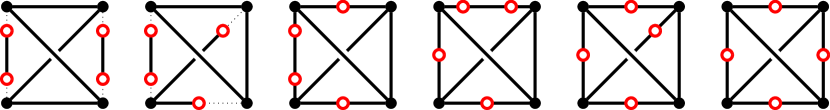
Figure 1. Log canonical surfaces with ample $K_{X}$

Proof.

This is a straightforward enumeration of the cases. There are only 8 cases satisfying Corollary 5.3. One of them is ${\mathbb{P}}^{2}$ with 4 lines, so that $-K_{X}$ is ample, and another one has $K_{X}=0$. The 6 listed cases are all legal and do appear. ∎

Lemma 5.5.

Let $f\colon Y\rightarrow\mathbb{P}^{2}$ be a sequence of blow-ups over the nodes of four lines $L=\sum L_{i}$, and $g\colon Y\rightarrow X$ the contraction of some visible curves, including $f^{-1}_{*}L$ but not any of the $(-1)$-curves, such that $K_{X}$ is log canonical and ample. Then each survivor is the image of a $(-1)$-curve on $Y$.

Proof.

Let $B_{0}\subset X$ be a survivor and $E_{0}$ its strict transform of $B_{0}$ on $Y$. Since $g$ contracts $f_{*}^{-1}L$, the curve $E_{0}$ is $f$-exceptional. To see that $E_{0}$ is a $(-1)$-curve, it suffices to show that there is no other $f$-exceptional curve over $E_{0}$: otherwise let $\pi\colon Y\rightarrow Y^{\prime}$ be the contraction of all the $f$-exceptional curves over $E_{0}$. Then $Y^{\prime}$ is smooth and $f\colon Y\rightarrow\mathbb{P}^{2}$ factors through some morphism $f^{\prime}\colon Y^{\prime}\rightarrow\mathbb{P}^{2}$. The log canonical divisor $\pi_{*}(g^{*}K_{X})$ is canonical along the divisor $E^{\prime}_{0}:=\pi_{*}E_{0}$. It follows that $\pi^{*}\pi_{*}(g^{*}K_{X})=g^{*}K_{X}$, and hence $g\colon Y\rightarrow X$ factors through $\pi\colon Y\rightarrow Y^{\prime}$, contradicting the assumption that $g$ is the minimal resolution. ∎

Lemma 5.6.

Let $X_{1},X_{2}$ be two log canonical surfaces with ample canonical class, and let $g_{n}\colon Y_{n}\to X_{n}$ be their minimal resolutions ($n=1,2$). Assume that there exists a (non identity) morphism $\pi:Y_{2}\to Y_{1}$ mapping the four survivors $E_{2}^{i}$ to the four survivors $E_{1}^{i}$ ($1\leq i\leq 4$) in such a way that the LR sequence for each $E_{2}^{i}$ prolongs that of $E_{1}^{i}$. Then one has $K_{X_{2}}^{2}>K_{X_{1}}^{2}$.

Proof.

Let $C_{n}$ be the union of all the curves contracted by $g_{n}$ ($n=1,2$). Then $\operatorname{vol}(K_{X_{n}})=\operatorname{vol}(K_{Y_{n}}+C_{n})$ and $C_{1}<\pi_{*}C_{2}$. Since $(Y_{1},C_{1})$ is canonical at the points blown up by $\pi$ and $C_{1}<\pi_{*}C_{2}$, one has $\pi^{*}(K_{Y_{1}}+C_{1})\leq K_{Y_{2}}+\pi_{*}^{-1}C_{1}<K_{Y_{2}}+C_{2}.$ It follows that

$$\operatorname{vol}(K_{X_{1}})=\operatorname{vol}(K_{Y_{1}}+C_{1})<\operatorname{vol}(K_{Y_{2}}+C_{2})=\operatorname{vol}(K_{X_{2}}).$$

∎

Theorem 5.7.

In the 6 cases of Fig. 1, the minimal $K_{X}^{2}$ are as in Table 1, achieved for the listed weight matrices. In particular, the absolute minimum is $1/6351$.

Case	Min $K^{2}$	Achieved at the weight matrix $W$
1	1/143	[[2, 1, 0, 0], [1, 7, 0, 0], [0, 0, 3, 1], [0, 0, 1, 4]]
2	1/143	[[2, 1, 0, 0], [1, 7, 0, 0], [1, 0, 2, 0], [1, 0, 0, 3]]
3	1/5537	[[5, 1, 0, 0], [1, 10, 0, 0], [1, 0, 0, 3], [0, 1, 2, 0]]
4	1/5537	[[2, 1, 0, 0], [1, 0, 0, 2], [0, 10, 1, 0], [0, 1, 5, 0]]
5	1/6351	[[1, 2, 0, 0], [9, 0, 1, 0], [1, 0, 0, 5], [0, 1, 2, 0]]
6	1/6351	[[1, 2, 0, 0], [0, 1, 2, 0], [0, 0, 1, 4], [10, 0, 0, 1]]

Table 1. Minimum $K_{X}^{2}$ in the 6 cases

Proof.

At each of the corners in Fig. 1 one can have a singularity with a fork, of type $D$ or $E$. However, by the classification recalled in the introduction, the cases for the determinants of the chains out of the fork are 1, 2, 3, 4, 5, 6, or $n\geq 7$, and the possibilities for any $n\geq 7$ are the same as for $7$.

We thus have finitely many possibilities for the weights $1\leq w_{i},w_{j}\leq 7$ on each edge $\{v_{i},v_{j}\}$. For each of them and for each fork, we have a condition that the singularity must be log canonical. The formula for the log discrepancy at a vertex was given in [Ale92] and is as follows (here, $\deg(v)$ is the valency of the vertex $v$):

$$c(u)=\frac{1}{\det\Gamma}\sum_{v\in{\rm Vert}(\Gamma)}\big{(}2-\deg(v)\big{)}\cdot\det\big{(}\Gamma-{\rm path}(u,v)\big{)}$$

For log canonical, one must have $c(u)\geq 0$ for each of the 4 corners in the graph. Using this formula, for each of the cases, we get finitely many series that depend on $0\leq p\leq 4$ parameters $x_{i}$. In cases 1 and 2 there is only one series up to symmetry, case 3: 2, case 4: 3, case 5: 60, and case 6: 18 series, for a total of 85 series.

Lemma 5.6 allows us to reduce the proof to checking finitely many cases. In each series the weight vectors of the survivors are either constant or are of the form $(n,k)\in{\mathbb{Z}}_{i}\times{\mathbb{Z}}_{j}$ where $k\in\{1,\dotsc,6\}$ is fixed and $n\to\infty$, subject to the condition that $(n,k)=1$. If $k=1$ then as in Example 3.6(2), the LR sequence is $L^{n-1}$. So once $K_{X}$ is ample for a certain surface in the series, increasing $n$ only makes $K_{X}^{2}$ larger.

If $k=2$ then the LR sequence for the weight $(2n-1,2)$ is $L^{n-1}R$. This is preceded by the sequence $L^{n-1}$ for the weight $(n,1)$. Once the canonical class for the latter sequence is ample, all the other surfaces obtained by increasing $n$ in the weight $(2n-1,2)$ will have a larger volume. Note also that if the surface for $(2n-1,2)$ is log canonical then so is the surface for $(n,1)$.

For the weight $(3n-1,3)$ the sequence is $L^{n-1}RL$, and for $(3n-2,3)$ it is $L^{n-1}R^{2}$. Once again, these are preceded by a log canonical surface with the weight $(n,1)$ and once for large enough $n$ the latter surface has ample $K_{X}$, the rest of the series is redundant. The cases $k=4,5,6$ are done entirely similarly. We are thus reduced to finitely many cases, which we checked using Theorem 4.2 and a sage [Sage] script. This concludes the proof. Even though it is redundant, below is an alternative way to reduce to finitely many checks.

As above, we get finitely many series of surfaces appearing in cases 1–6. Let us work with one of them: $\{X(n_{1},\dotsc,n_{p})\}$, depending on $p\leq 4$ parameters. There are only finitely many minimal, in the lexicographic order, sequences $(n_{1},\dotsc,n_{p})$ for which $K_{X}$ is ample, i.e. $\det{\widehat{W}}(n_{1},\dotsc,n_{p})>0$ in Theorem 4.2. We claim that it is sufficient to seek the minimum $K_{X}^{2}$ among these minimal sequences plus a few more. By Lemma 5.6, for each survivor of the form $(n,1)$, increasing $n$ makes $K^{2}$ larger. By looking at the 85 series, we observe that at most one of the weight vectors $(n_{s},k_{s})$ has $k_{s}\geq 2$, say $k_{1}\geq 2$. We deal with this vector differently.

Let us denote $x=n_{1}$. By (4.2) the function $f(x)=K^{2}(x)$ up to a constant has the form $\frac{(x-a)^{2}}{(x-b)^{2}+c}$. From the fact that in Theorem 5.4 no surface with ample $K_{X}$ has survivors in the corners, by row expansion of $\det{\widehat{W}}$ it follows that $a\geq 0$. By the general theory of [Ale94], the function $K^{2}(x)$ is increasing for $x\gg 0$. This gives $a\geq b$. By computing the derivative $f^{\prime}(x)$ one easily sees that if $f(x+1)\geq f(x)$ then $f(y+1)\geq f(y)$ for any $y\geq x$. Thus, for each of the minimal sequences $(n_{1},n_{2},\dotsc,n_{p})$ it suffices to check that $K^{2}(n_{1}+1,n_{2},\dotsc,n_{p})\geq K^{2}(n_{1},n_{2},\dotsc,n_{p})$. We performed this check as well. ∎

Remark 5.8.

For the best surface in case 2, the surface $Y$ as in (1.1) is obtained from the one in case 1 by contracting a $(-1)$-curve. Thus, in fact the surfaces $X$ with ample $K_{X}$ are the same. We showed in [AL16] that the surfaces in cases 5 and 6 are isomorphic, only the presentations with the visible curves are different. Similarly, one can show that the best surfaces in cases 3 and 4 are isomorphic.

Remark 5.9.

In each of the subcases of the main six cases, the series depend on $0\leq p\leq 4$ parameters. The series with the maximal number of 4 parameters are given in Table 2 and depicted in Fig. 2.

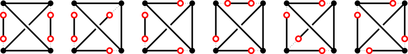
Figure 2. The 4-parameter series

Case	Weight matrix $W$
1	$[[x_{1},1,0,0],\ [1,x_{2},0,0],\ [0,0,x_{3},1],\ [0,0,1,x_{4}]]$
2	$[[x_{1},1,0,0],\ [1,x_{2},0,0],\ [1,0,x_{3},0],\ [1,0,0,x_{4}]]$
3	$[[x_{1},1,0,0],\ [1,x_{2},0,0],\ [1,0,0,x_{3}],\ [0,1,x_{4},0]]$
4	$[[x_{1},1,0,0],\ [1,0,0,x_{2}],\ [0,x_{3},1,0],\ [0,1,x_{4},0]]$
5	$[[1,x_{1},0,0],\ [x_{2},0,1,0],\ [1,0,0,x_{3}],\ [0,1,x_{4},0]]$
6	$[[1,x_{1},0,0],\ [0,1,x_{2},0],\ [0,0,1,x_{3}],\ [x_{4},0,0,1]]$

Table 2. Weight matrices in the 4-parameter series

In these 4-parameter series, all singularities are of the $A$ type, i.e. correspond to chains only. (In the series with fewer parameters, forks do appear.) Using Corollary 2.6, here are the explicit formulas for the determinants of the singularities:

1. $\Delta=|x_{1},x_{2}|\cdot|x_{3},x_{4}|\cdot|x_{1}-1,x_{3}-1,x_{2}-1,x_{4}-1,\circlearrowleft|$.

2. $\Delta=|x_{1},x_{2}|\cdot|-x_{3},x_{1}-1,-x_{4}|\cdot|x_{2}-1,x_{3}-1,x_{4}-1,\circlearrowleft|$.

3. $\Delta=|x_{1},x_{2}|\cdot|-x_{4},x_{1}-1,x_{3}-1,x_{4}-1,x_{2}-1,-x_{3}|$.

4. $\Delta=|x_{2},x_{3}|\cdot|-x_{4},x_{1}-1,x_{3}-1,x_{4}-1,x_{2}-1,-x_{1}|$.

5. $\Delta=|-x_{1},x_{3}-1,-x_{4}|\cdot|-x_{2},x_{1}-1,x_{4}-1,x_{2}-1,-x_{3}|$.

6. $\Delta=|-x_{1},x_{4}-1,x_{2}-1,-x_{3}|\cdot|-x_{2},x_{1}-1,x_{3}-1,-x_{4}|$.

In every series, both the numerator and denominator in $K_{X}^{2}=\frac{(\det{\widehat{W}})^{2}}{\Delta}$ is a polynomial of multidegree $(2,2,2,2)$ in the variables $x_{1},x_{2},x_{3},x_{4}$ with the leading term $x_{1}^{2}x_{2}^{2}x_{3}^{2}x_{4}^{2}$, and the limit of $K_{X}^{2}$ as all $x_{i}\to\infty$ is 1.

6. Pairs $(X,B)$ with reduced $B$, and limit points of volumes

Theorem 6.1.

For the the log canonical pairs $(X,B)$ with reduced nonempty divisor $B$ there are the 12 cases of Fig. 3, plus $({\mathbb{P}}^{2},\sum_{k=1}^{4}L_{k})$. The minimal $(K_{X}+B)^{2}$ for these cases are as in Table 3, achieved for the listed weight matrices. In particular, the absolute minimum for the volume in these settings is $1/78$.

The proof is the same as for Theorem 5.7.

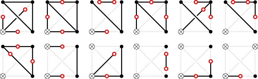
Figure 3. Log canonical pairs with ample $K_{X}+B$, reduced $B\neq 0$

Case	Min $(K+B)^{2}$	Achieved at the weight matrix $W$
1	1/42	[[1, 0, 0, 0], [1, 2, 0, 0], [1, 0, 3, 0], [1, 0, 0, 7]]
2	1/78	[[1, 0, 0, 0], [1, 2, 0, 0], [1, 0, 0, 3], [0, 1, 4, 0]]
3	1/22	[[1, 0, 0, 0], [1, 0, 0, 2], [0, 3, 1, 0], [0, 1, 4, 0]]
4	1/70	[[1, 0, 0, 0], [1, 2, 0, 0], [0, 1, 2, 0], [0, 0, 1, 4]]
5	1/22	[[1, 0, 0, 0], [1, 0, 2, 0], [0, 2, 1, 0], [0, 0, 1, 3]]
6	1/15	[[1, 0, 0, 0], [0, 3, 1, 0], [0, 1, 2, 0], [0, 0, 1, 2]]
7	1/60	[[1, 0, 0, 0], [0, 1, 2, 0], [0, 2, 0, 1], [0, 0, 1, 3]]
8	1/6	[[1, 0, 0, 0], [0, 1, 0, 0], [1, 0, 0, 2], [0, 1, 3, 0]]
9	1/6	[[1, 0, 0, 0], [0, 1, 0, 0], [1, 0, 2, 0], [1, 0, 0, 3]]
10	1/3	[[1, 0, 0, 0], [0, 1, 0, 0], [0, 0, 2, 1], [0, 0, 1, 2]]
11	1/6	[[1, 0, 0, 0], [0, 1, 0, 0], [1, 0, 0, 2], [0, 0, 2, 1]]
12	1/2	[[1, 0, 0, 0], [0, 1, 0, 0], [0, 0, 1, 0], [1, 0, 0, 2]]
13	1	[[1, 0, 0, 0], [0, 1, 0, 0], [0, 0, 1, 0], [0, 0, 0, 1]]

Table 3. Minimum $(K_{X}+B)^{2}$ in the 13 cases

Theorem 6.2.

Let $(X_{n},B_{n})$, $n\geq n_{0}$ be a series of log canonical pairs with ample $K_{X_{n}}+B_{n}$ in which one of the survivors has the weight vector $\vec{w}(n)=(n,k,0,0)$ with $n\to\infty$, and the other weights and log discrepancies $c_{i}$ of the survivors are fixed. Then the limit of the volumes $(K_{X_{n}}+B_{n})^{2}$ is $(K_{{\overline{X}}}+{\overline{B}})^{2}$ where the pair $({\overline{X}},{\overline{B}})$ is obtained by replacing $\vec{w}(n)$ by $(1,0,0,0)$ and setting the log discrepancy $\bar{c}_{1}=0$. In other words, $L_{1}$ is a survivor for ${\overline{X}}$ and it appears in ${\overline{B}}$ with coefficient $b_{1}=1$.

Proof.

By Theorem 4.2, we have $(K_{X}+B)^{2}=\frac{(\det{\widehat{W}})^{2}}{\Delta}$. The function $\det{\widehat{W}}(X_{n})$ is linear in $n$, with the leading coefficient equal to the determinant of the matrix obtained by replacing the row $(n,k,0,0;c)$ by $(1,0,0,0;0)$. The determinant $\Delta(X_{n})$ for the singularities is a quadratic function of $n$ and it easily follows from the formulas in (2.7), (3.11) that the coefficient of $n^{2}$ is $\Delta({\overline{X}})$. Thus,

$$\lim_{n\to\infty}\frac{\big{(}\det{\widehat{W}}(X_{n})\big{)}^{2}}{\Delta(X_{n})}=\frac{\big{(}\det{\widehat{W}}({\overline{X}})\big{)}^{2}}{\Delta({\overline{X}})}.$$

∎

Corollary 6.3.

The smallest limit point for the log canonical pairs $(X,B)$ with coefficients in $\{0,1\}$ with $\rho(X)=1$ obtained from the four-line configuration is $1/78$.

Proof.

Indeed, the minimal volume $\frac{1}{78}$ in case 2 of Table 3 appears as the limit of the volumes in case 5 of Table 2 for $x_{1}=2$, $x_{3}=3$, $x_{4}=4$ and $x_{2}\to\infty$. ∎

We conclude with the following:

Lemma 6.4.

The set ${\mathbb{K}}^{2}=\{K_{X}^{2}\}$ of volumes of log canonical surfaces obtained via Construction 1.1 has accumulation complexity 4, i.e. $\operatorname{Acc}^{4}({\mathbb{K}}^{2})\neq\emptyset$, $\operatorname{Acc}^{5}({\mathbb{K}}^{2})=~{}\emptyset$, where $\operatorname{Acc}^{0}({\mathbb{K}}^{2})={\mathbb{K}}^{2}$ and $\operatorname{Acc}^{n+1}({\mathbb{K}}^{2})$ is the set of accumulation points of $\operatorname{Acc}^{n}({\mathbb{K}}^{2})$.

Proof.

Indeed, in the proof of Theorem 5.7 we produced finitely many (85 to be exact) series of surfaces $X(n_{1},\dotsc,n_{p})$ that depend on $p\leq 4$ integer parameters. Sending any of $n_{i}\to\infty$ gives an accumulation point, sending $n_{j}\to\infty$ for $n_{j}\neq n_{i}$ gives a point in $\operatorname{Acc}^{2}({\mathbb{K}}^{2})$, etc. ∎

References

- [AL16] Valery Alexeev and Wenfei Liu, Open surfaces of small volume, Algebraic Geometry, to appear (2016), arXiv:1612.09116.
- [AL18] Valery Alexeev and Wenfei Liu, On accumulation points of volumes of log surfaces, Izv. Ross. Akad. Nauk Ser. Mat., to appear (2018), arXiv:1803.09582.
- [Ale92] Valery Alexeev, Log canonical surface singularities: arithmetical approach, Flips and abundance for algebraic threefolds, Société Mathématique de France, Paris, 1992, Papers from the Second Summer Seminar on Algebraic Geometry held at the University of Utah, Salt Lake City, Utah, August 1991, Astérisque No. 211 (1992), pp. 47–58.
- [Ale94] by same author, Boundedness and for log surfaces, Internat. J. Math. 5 (1994), no. 6, 779–810.
- [AM04] Valery Alexeev and Shigefumi Mori, Bounding singular surfaces of general type, Algebra, arithmetic and geometry with applications (West Lafayette, IN, 2000), Springer, Berlin, 2004, pp. 143–174.
- [Sage] The Sage Developers, Sagemath, the Sage Mathematics Software System (Version 7.5.1), 2017, http://www.sagemath.org.