Inaccuracy of Spatial Derivatives in Simulations of Supersonic Turbulence

Abstract

We examine the accuracy of spatial derivatives computed from numerical simulations of supersonic turbulence. Two sets of simulations, carried out using a finite-volume code that evolves the hydrodynamic equations with an approximate Riemann solver and a finite-difference code that solves the Navier-Stokes equations, are tested against a number of criteria based on the continuity equation, including exact results at statistically steady state. We find that the spatial derivatives in the Navier-Stokes runs are accurate and satisfy all the criteria. In particular, they satisfy our exact results that the conditional mean velocity divergence, $\langle\nabla\cdot{\boldsymbol{u}}|s\rangle$, where $s$ is the logarithm of density, and the conditional mean of the advection of $s$, $\langle{\boldsymbol{u}}\cdot\nabla s|s\rangle$, vanish at steady state for all density values, $s$. On the other hand, the Riemann solver simulations fail all the tests that require accurate evaluation of spatial derivatives, resulting in apparent violation of the continuity equation, even if the solver enforces mass conservation. In particular, analysis of the Riemann simulations may lead to the incorrect conclusion that the $p\,dV$ work tends to preferentially convert kinetic energy into thermal energy, inconsistent with the exact result that the energy exchange by $p\,dV$ work is symmetric in barotropic supersonic turbulence at steady state. The inaccuracy of spatial derivatives is a general problem in the post-processing of simulations of supersonic turbulence with Riemann solvers. Solutions from such simulations must be used with caution in post-processing studies concerning the spatial gradients.

1. Introduction

Numerical simulations are a powerful tool for turbulence studies and have driven major advances in our knowledge of highly compressible turbulence in the interstellar medium. Through visualization and statistical analysis, numerical simulations have helped capture and quantify the complicated density and velocity structures in supersonic interstellar turbulence, offering physical insight for the interpretation of observational results. In particular, numerical experiments have played a crucial role in the theoretical modeling of the process of star formation in molecular clouds (e.g. Padoan et al. 2014).

The limited spatial resolution is still a major challenge for the interpretation of numerical simulations of turbulence, because the effective Reynolds number of even the largest simulations is still orders of magnitude lower than that in interstellar clouds. Many astrophysical simulations do not even reach a broad enough dynamical range of scales to allow the development of an inertial range of turbulence (let alone to describe the turbulent fragmentation process down to the sonic scale). In order to maximize the inertial range, the strategy of choice in supersonic turbulence is to use Riemann solvers to evolve the integral form of the Euler equations rather than the Navier-Stokes equations, based on the assumption that the inertial-range dynamics is insensitive to the exact form of the viscosity (following Kolmogorov’s universality hypothesis for the inertial-range properties of turbulence, e.g., Frisch 1995). In such simulations, energy dissipation occurs only implicitly, without an explicit viscous term, and the simulated flow may acquire an effective Reynolds number significantly larger than in corresponding Navier-Stokes simulations. For convenience we refer to such simulations as ‘Euler simulations’ in this paper, even though the solutions of course—especially in the supersonic context—would not exist without the implicit viscosity present in the Riemann solver, and ‘Navier-Stokes solutions with implicit sub-grid viscosity’ would be a more precise label. These simulations are also referred to as implicit large-eddy simulations (ILES) in the numerical literature.

Without an explicit physical viscosity in Euler simulations, velocity and density profiles in sharp discontinuities are completely determined by the numerical algorithm (e.g. choice of Riemann solvers) and the specific methods to achieve numerical stability (e.g. choice of slope limiters). The resulting profile shapes within the discontinuities are numerically stable and the resulting solutions strictly obey the conservation laws, but with fluxes of mass, momentum, and total energy that are modified on the cell scale, relative to fluxes computed directly from the conserved variables. The extent to which this numerical approach affects diagnostics that rely on small-scale spatial derivatives of the flow quantities has not been carefully addressed so far. The goal of this work is to quantify the consequence of such inaccuracies in simulations of supersonic turbulence without explicit viscosity, which may have a significant impact for a large number of numerical studies.

Spatial derivatives are indeed often needed in the statistical analysis of turbulence simulation data. The velocity gradient tensor and its three components, namely the rate of strain tensor, the vorticity, and the divergence are of great theoretical interest and have been extensively investigated in turbulence studies. In compressible turbulence, the statistics of vorticity and divergence are useful measures to characterize the solenoidal and compressible parts of the velocity field (e.g., Porter et al. 2002, Pavlovski et al. 2006, Wang et al. 2011). Furthermore, there is a wide range of important physical quantities related to the velocity gradient. Examples include, but are not limited to, the enstrophy, the Taylor microscale (Porter et al. 1992a,b, Kritsuk et al. 2007), the helicity (Porter et al. 1992b, Kritsuk et al. 2007), the energy dissipation rate (e.g., Kritsuk et al. 2007, Pan & Padoan 2009, Pan et al. 2009), the small-scale compressive ratio (Kida & Orszag 1990, 1992, Porter et al. 1992a,b, Kritsuk et al. 2007), the pressure-dilatation interactions or the $p\,dV$ work (Porter et al. 1998, Pan & Scannapieco 2010, Aluie et al.  2012). The velocity gradient is also needed to study the preferential alignment of the vorticity with the principle directions of the strain tensor (e.g., Porter et al. 1998, Sur et al. 2013). The analysis of all the above physical quantities relies on accurate computation of the spatial derivative of the velocity field, yet many of the works cited above are based on Euler simulations, where velocity gradients may suffer from numerical artifacts.

Although it should be straightforward to realize that spatial derivatives from simulations without explicit viscosity may be inaccurate at discontinuities, to our knowledge, the issue has so far not been carefully examined. It may have been overlooked because of the overwhelming interest in understanding the inertial-range dynamics of supersonic turbulence, rather than in achieving accurate small-scale statistics, or because of the lack of an objective criterion to quantify numerical errors in the computed spatial derivatives. In this work, we examine spatial derivatives in simulations of supersonic turbulence using a number of criteria, including exact results we have previously derived from the continuity equation at steady state (Pan et al. 2018). We show that the spatial derivatives in the Euler simulations are not reliable, especially in dense regions. In contrast, in simulations that evolve the Navier-Stokes equations, spatial derivatives are found to be accurate.

In §2, we outline the criteria used to test the accuracy of spatial derivatives in numerical simulations. §3 examines spatial derivatives in two sets of simulations, which are carried out using two different numerical codes with and without an explicit viscous term. Implications of our results are discussed in §4, and the main conclusions of the study are summarized in §5.

2. Criteria to test spatial derivatives

We start by writing down the continuity equation,

$$\frac{\partial\rho}{\partial t}+\nabla\cdot(\rho\boldsymbol{u})=0,$$ (1)

and the momentum equation,

$$\frac{\partial(\rho\boldsymbol{u})}{\partial t}+\nabla\cdot(\rho\boldsymbol{u}\boldsymbol{u})=-\nabla p+\nabla\cdot\mathcal{\sigma}+\rho{\boldsymbol{a}},$$ (2)

where $\sigma$ denotes the viscous stress tensor, and ${\boldsymbol{a}}$ is the acceleration that drives the turbulent flow. All other symbols carry their conventional meanings. In most simulations of supersonic turbulence the viscous term, $\nabla\cdot\mathcal{\sigma}$, in the momentum equation is neglected, in order to minimize the thickness of discontinuities and achieve the largest possible effective Reynolds number. However, such sharp discontinuities are numerically unstable. The necessary corrections to the profile of the flow variables within the discontinuities to obtain the desired stability, such as flux or slope limiters or various forms of explicit numerical dissipation yield inaccurate spatial derivatives in the discontinuities.

We will evaluate the uncertainties in the spatial derivatives computed from simulation data using a number of criteria. A simple test is to check whether and how well the continuity equation is satisfied with density and velocity derivatives computed from the data. For convenience, we rewrite Eq. (1) as,

$$\frac{\partial s}{\partial t}+\boldsymbol{u}\cdot\nabla s+\nabla\cdot\boldsymbol{u}=0,$$ (3)

where $s\equiv\ln(\rho/\bar{\rho})$ is the logarithm of the density, $\rho$, with $\bar{\rho}$ being the mean density.

In a perfect numerical simulation, one would expect that Eq. (3) is exactly satisfied. It may seem trivial that, as long as mass conservation is enforced in the simulation, Equation (1) and, by inference, Equation (3) should hold exactly. That is, however, not true, if the numerical schemes involve flow corrections designed to stabilize shocks, as such corrections introduce errors in the spatial derivatives, even while enforcing mass conservation. As a consequence, the density and velocity fields from an Euler simulation may appear to not satisfy the continuity equation, Equation (1), and the three terms in Eq. (3) may not add up to zero when evaluated with finite-difference derivatives of density and velocity, even if the code strictly enforces mass conservation. This apparent contradiction has a simple explanation: a generic finite-volumes Euler code does not require those spatial derivatives to evolve the flow solution (the code does not solve the continuity equation in the differential form of Eq. (3), but solves an integral form of Eq. (1)), so the solution is evolved correctly and satisfies the conservation laws despite the incorrect spatial derivatives.

To quantify this potential problem, we consider the sum of the three terms of the continuity equation, which we refer to as the numerical or artificial residual of the continuity equation and denote as $R=\partial_{t}s+\boldsymbol{u}\cdot\nabla s+\nabla\cdot\boldsymbol{u}$. In the following section, we check whether $R$ is zero point-wise on the simulation grid, and, if not, find out where deviations typically occur. We also test statistically how well Eq. (3) is satisfied in flow regions at different density. The test is carried out by computing the averages of the three terms in Eq. (3), conditioned on the local flow density, denoted as $\langle\partial_{t}s|s\rangle$, $\langle\nabla\cdot\boldsymbol{u}|s\rangle$ and $\langle\boldsymbol{u}\cdot\nabla s|s\rangle$, respectively. Here $\langle\cdot\cdot\cdot|s\rangle$ represents the average over the flow regions at a given value of $s$. Obviously, if Eq. (3) held perfectly, we would have $\langle R|s\rangle=0$ or,

$$\langle\partial_{t}s|s\rangle+\langle\boldsymbol{u}\cdot\nabla s|s\rangle+\langle\nabla\cdot\boldsymbol{u}|s\rangle=0,$$ (4)

at each density level. A test based on this equation can tell us at which density the spatial derivatives computed from a simulation are more (or less) reliable.

In addition to directly testing spatial derivatives against the continuity equation, we also consider several other criteria based on exact results derived from the continuity equation at statistically steady state. We outline such criteria in the following subsections.

2.1. Time derivative of $s$

At statistically steady state, the average, $\langle s\rangle$, of $s$ becomes time-independent, and it is expected that $\langle\partial_{t}s\rangle=\partial_{t}\langle s\rangle=0$. The assumption of steady state has stronger implications than $\langle\partial_{t}s\rangle=0$. In fact, assuming that the probability distribution of $s$ is invariant with time at steady state, one can show that the conditional average of $\partial_{t}s$ on the density is zero at each density level. Our proof begins with defining a fine-grained PDF of $s$ as $g(\zeta;{\boldsymbol{x}},t)=\delta(\zeta-s({\boldsymbol{x}},t))$, where $\delta$ is the Dirac delta function and $\zeta$ the sampling variable. The time derivative $g$ is given by,

$$\frac{\partial g(\zeta;{\boldsymbol{x}},t)}{\partial t}=-\frac{\partial(g\partial_{t}s)}{\partial\zeta},$$ (5)

where we used the fact that $\partial_{t}s$ is independent of the sampling variable $\zeta$ for the term on the right hand side.

We then define the coarse-grained PDF as the average of the fine-grained PDF, i.e., $f(\zeta;t)\equiv\langle g(\zeta;{\boldsymbol{x}},t)\rangle=V^{-1}\int_{V}\delta(\zeta-s({\boldsymbol{x}},t)d^{3}x$, where the integral is over the volume, $V$, of the entire flow domain. For any flow quantity $\phi({\boldsymbol{x}},t)$, it can be shown that $\langle\phi({\boldsymbol{x}},t)g(\zeta;{\boldsymbol{x}},t)\rangle=\langle\phi({\boldsymbol{x}},t)\delta(\zeta-s({\boldsymbol{x}},t))\rangle=\langle\phi|s=\zeta\rangle f(\zeta;t)$, where $\langle\phi|s=\zeta\rangle$ is the average of $\phi$ over all the flow regions where $s({\boldsymbol{x}},t)$ equals the sampling variable (Pope 2000). Averaging Eq. (5) then gives,

$$\frac{\partial f(\zeta;t)}{\partial t}=-\frac{\partial(\langle\partial_{t}s|s=\zeta\rangle f)}{\partial\zeta},$$ (6)

and further assuming steady state, we have $\partial_{\zeta}(\langle\partial_{t}s|s=\zeta\rangle f)=0$. Therefore, $\langle\partial_{t}s|s=\zeta\rangle f=C_{1}$, with $C_{1}$ the integration constant. Considering that $\int_{-\infty}^{\infty}\langle\partial_{t}s|s=\zeta\rangle fd\zeta=\langle\partial_{t}s\rangle$, which vanishes at steady state, the constant $C_{1}$ must be zero, and we obtain,

$$\langle\partial_{t}s|s=\zeta\rangle=0,$$ (7)

meaning that the conditional mean of the time derivative of $s$ is zero at any density. The only assumption made in the derivation is that the coarse-grained PDF is time independent, i.e., $\partial_{t}f(\zeta;t)=0$, which is expected once the flow reaches steady state. Equation (7) will be used to check whether the simulated flow has reached steady state.

For simplicity of notations, in the rest of the paper, we will drop the sampling variable, $\zeta$, in the conditional means, and write $\langle...|s=\zeta\rangle$ simply as $\langle...|s\rangle$. The density PDF will be written as $f(s;t)$ accordingly.

2.2. Exact results of Pan et al. (2018)

Pan et al. (2018) derived two exact results from the continuity equation under the assumption of statistical stationarity and homogeneity. We briefly review the derivation here and refer the interested reader to Pan et al. (2018) for more details.

At steady state, it follows from Eqs. (4) and (7) that,

$$\langle\boldsymbol{u}\cdot\nabla s|s\rangle+\langle\nabla\cdot\boldsymbol{u}|s\rangle=0.$$ (8)

In Pan et al. (2018), the two terms were referred to as the conditional mean advection and conditional mean divergence, respectively. Using periodic boundary conditions (which is equivalent to the assumption of statistical homogeneity in Pan et al. 2018), the two terms are related to each other by,

$$\langle\nabla\cdot\boldsymbol{u}|s\rangle f=\frac{\partial}{\partial s}\Big{(}\langle\boldsymbol{u}\cdot\nabla s|s\rangle f\Big{)}.$$ (9)

Combining Eqs. (8) and (9) yields,

$$\frac{\partial}{\partial s}\Big{(}\langle\nabla\cdot\boldsymbol{u}|s\rangle f\Big{)}+\langle\nabla\cdot\boldsymbol{u}|s\rangle f=0,$$ (10)

which is solved by $\langle\nabla\cdot\boldsymbol{u}|s\rangle f(s)=C_{2}\exp(-s)$ with $C_{2}$ being the integration constant. Because $\int_{-\infty}^{\infty}\langle\nabla\cdot\boldsymbol{u}|s\rangle f(s)ds=\langle\nabla\cdot\boldsymbol{u}\rangle=0$, the constant $C_{2}$ must vanish, and we have,

$$\langle\nabla\cdot\boldsymbol{u}|s\rangle=0,$$ (11)

meaning that the divergence in expanding and contracting regions at any given density exactly cancels out.

Combining Eqs. (9) and (11) yields $\langle\boldsymbol{u}\cdot\nabla s|s\rangle f=C_{3}$ where $C_{3}$ is another integration constant. The integral of $\langle\boldsymbol{u}\cdot\nabla s|s\rangle f$ over the $s-$space is equal to $\langle\boldsymbol{u}\cdot\nabla s\rangle$. By averaging Eq. (3) and using statistical homogeneity, it is straightforward to see that $\langle\boldsymbol{u}\cdot\nabla s\rangle=0$ at steady state. This requires $C_{3}=0$, leading to the second exact result of Pan et al. (2018),

$$\langle\boldsymbol{u}\cdot\nabla s|s\rangle=0.$$ (12)

Pan et al. (2018) used the exact results, Eqs. (11) and (12), to test potential numerical artifacts in Euler simulations of supersonic turbulence. In §3, we will further test the spatial derivatives in simulated turbulent flows using both Euler and Navier-Stokes simulations.

We stress that the derivation in §2.1 for $\langle\partial_{t}s|s\rangle=0$ only assumed steady state, while here the derivation of Eqs. (11) and (12) requires both statistical stationarity and homogeneity (through the use of periodic boundary conditions). The results in §2.1 and 2.2 show that, if the continuity equation is perfectly satisfied, each of the three terms in Eq. (4) is zero at steady state. On the other hand, if the continuity equation does not hold exactly, Eq. (4) breaks down, and at least one of the three terms is nonzero. Each of the three terms will be examined in §3.

2.3. The $p\,dV$ work

Kinetic energy and thermal energy in a turbulent flow may be converted into each other through $p\,dV$ work. Unlike viscous dissipation, which is a one-way conversion of kinetic energy into heat, the energy exchange by $p\,dV$ work is reversible, and its rate $p\nabla\cdot{\boldsymbol{u}}$ can be either positive or negative. An interesting question is whether the two-way energy exchange by $p\,dV$ work is symmetric in supersonic turbulence. In other words, does the energy conversion by $p\,dV$ work have a preferred direction, causing a net energy flow from one form of energy to the other? To answer the question, one may compute the average $p\,dV$ work, $\langle p\nabla\cdot{\boldsymbol{u}}\rangle$, over the flow domain and check if it is positive, negative or zero. Clearly, due to its dependence on the divergence, an accurate evaluation of $p\,dV$ work requires reliable spatial derivatives of the velocity field.

Previous numerical studies found that the energy exchange by $p\,dV$ work in isothermal, supersonic turbulence is asymmetric. At steady state, $\langle p\nabla\cdot{\boldsymbol{u}}\rangle$ was found to be negative, meaning that the $p\,dV$ work preferentially converts kinetic energy to heat (Pan & Scannapieco 2010, see also Kritsuk et al. 2013). However, this conclusion is questionable because the simulations used in those studies do not include explicit viscosity, and, as discussed earlier, the velocity divergence in such simulations may suffer from numerical artifacts.

2.3.1 Energy exchange by $p\,dV$ work is symmetric

In fact, under the assumption of statistical homogeneity, one can show that $\langle p\nabla\cdot{\boldsymbol{u}}\rangle$ must be zero at steady state if the turbulent flow is barotropic. For a barotropic fluid, the pressure is a function of the density only, i.e., $p=p(\rho)=p(s)$, and to prove $\langle p\nabla\cdot{\boldsymbol{u}}\rangle=0$, we define an auxiliary function, $h(s)\equiv\int^{s}p(s^{\prime})\exp(s-s^{\prime})ds^{\prime}$. It follows from Eq. (3) that ${\partial_{t}h}+\boldsymbol{u}\cdot\nabla h+h^{\prime}\nabla\cdot\boldsymbol{u}=0$, and, since $h(s)$ satisfies $h^{\prime}(s)-h(s)=p(s)$, we have,

$$\frac{\partial h}{\partial t}+\nabla\cdot(h\boldsymbol{u})=-p\nabla\cdot\boldsymbol{u}.$$ (13)

Averaging the equation and assuming statistical stationarity and homogeneity, we find $\langle p\nabla\cdot{\boldsymbol{u}}\rangle=0$, as claimed. This proves that the energy exchange by $p\,dV$ work is symmetric in barotropic turbulent flows.

For an adiabatic flow, $p\propto\rho^{\gamma}$, with $\gamma$ the ratio of specific heats, and $h={p}/({\gamma-1})$ is the thermal energy. Thus, the right hand side of Eq. (13) may be viewed as a source term for thermal energy, and $\langle p\cdot\nabla{\boldsymbol{u}}\rangle=0$ corresponds to the constancy of the average thermal energy, $\langle h\rangle$, at steady state. The isothermal equation of state, commonly adopted in simulations for supersonic turbulence in molecular clouds, is another example of barotropy, so it is expected that the average $p\,dV$ work in isothermal flows is also zero at steady state. For isothermal gas, $p=\rho C_{\rm s}^{2}$ with $C_{\rm s}$ the constant sound speed, and we have $h=C_{\rm s}^{2}\rho s$. Galtier and Banerjee (2011) suggested that $C_{\rm s}^{2}\rho s$ may be viewed as the effective thermal energy of isothermal gas. Clearly, $C_{\rm s}^{2}\rho s$ is not the real thermal energy of interstellar gas, which is given by the usual formula ${\rho C_{\rm s}^{2}}/{(\gamma-1)}$. Defining $h=C_{\rm s}^{2}\rho s$ as the effective thermal energy in isothermal flows was motivated by the fact that the total effective energy, defined as $\frac{1}{2}\rho u^{2}+C_{\rm s}^{2}\rho s$, is conserved by the advection and pressure terms. As an auxiliary variable, $h=C_{\rm s}^{2}\rho s$ is helpful for understanding the energy budget in supersonic turbulence with assumed isothermal equation of state.

From another perspective, Eq. (13) is also useful to understand density fluctuations in isothermal, supersonic turbulence. Since the sound speed is constant, $\langle h\rangle\propto\langle\rho s\rangle$, which increases with the width of the probability distribution function (PDF) of $s$. For example, if the PDF of $s$ is Gaussian with a standard deviation of $\sigma_{\rm s}$, we have $\langle\rho s\rangle=\sigma_{\rm s}^{2}/2$, suggesting that $\langle h\rangle$ may be used as a measure for the density PDF width. Therefore, the right hand side of Eq. (13) can be viewed as a source term for density fluctuations. When the density fluctuations develop from the initial condition, the source term must be positive on average to widen the density PDF. This implies that, as the density fluctuations develop, the $p\,dV$ work converts kinetic energy to the effective thermal energy. But once the flow reaches steady state, the conversion stops and the average $p\,dV$ work vanishes.

The method used above in the proof for zero average $p\,dV$ work at steady state is actually not restricted to the specific issue of $p\,dV$ work. In general, one can prove $\langle F\nabla\cdot{\boldsymbol{u}}\rangle=0$ for any function, $F(\rho)$, of density. For a power law function, $F\propto\rho^{n}$, we have $\langle\rho^{n}\nabla\cdot{\boldsymbol{u}}\rangle=0$ for any $n$, which corresponds to the fact that the $n$-th moment, $\langle\rho^{n}\rangle$, of the density PDF is constant when the flow reaches steady state.

2.3.2 Conditional average of the $p\,dV$ work

The result that the energy exchange by $p\,dV$ work in barotropic turbulent flows is symmetric at steady state can be further generalized using the exact relation, Eq. (11), in §2.2. Instead of considering the global average of the $p\,dV$ work, we now look at the conditional average, $\langle p\nabla\cdot{\boldsymbol{u}}|s\rangle$, of the $p\,dV$ work over flow regions at each given density level, $s$. Clearly, if the pressure is a function of density only, we have $\langle p(\rho)\nabla\cdot{\boldsymbol{u}}|s\rangle=\langle p(\exp(s))\nabla\cdot{\boldsymbol{u}}|s\rangle=p(\exp(s))\langle\nabla\cdot{\boldsymbol{u}}|s\rangle$. As Eq. (11) predicted that $\langle\nabla\cdot{\boldsymbol{u}}|s\rangle=0$ at steady state, it immediately follows that $\langle p\nabla\cdot{\boldsymbol{u}}|s\rangle=0$ at all values of $s$. We thus have reached a stronger conclusion: At steady state, the $p\,dV$ work does not cause a net energy exchange between kinetic and thermal energy in flow regions of any given density. In other words, the $p\,dV$ work is symmetric at each density level.

Due to the complicated heating and cooling mechanisms, the interstellar gas is not really isothermal or barotropic, so the predicted symmetry of the $p\,dV$ work based on the assumption of barotropy may not apply in general to interstellar turbulence. Nevertheless, the results in this section concerning the $p\,dV$ work provide a useful test for the accuracy of spatial derivatives computed from simulation data, and we use them to demonstrate the necessity of including explicit viscosity in order to accurately measure the velocity divergence in simulated flows.

3. Testing Spatial Derivatives in Numerical Simulations

We conducted two sets of simulations, one solving the Euler equations (without explicit viscosity), the other solving the Navier-Stokes equations (with explicit viscosity). Both sets of simulations are carried out with the Dispatch code (Nordlund et al., 2018), as it provides an efficient computing framework to test different fluid-dynamics solvers. The first set of experiments without an explicit viscous term adopted the HLLC (Harten-Lax-van Leer-Contact) approximate Riemann solver (Toro et al., 1994). They will be referred to as the Riemann runs. The second set of experiments adopted a simplified, 2nd order version of the 6th oorder solver in the Stagger Code (Galsgaard & Nordlund, 1996; Kritsuk et al., 2011; Baumann et al., 2012), including the viscous term in the Navier-Stokes (N-S) equations (Eq. (2)). We refer to these experiments with explicit viscosity as the N-S runs.

In the N-S runs, the viscous tensor, $\sigma_{ij}$, was set to $\sigma_{ij}=\rho\nu(\partial_{j}u_{i}+\partial_{i}u_{j})$, where $\nu$ is the kinematic viscosity. We assumed a kinematic viscosity, $\nu=\Delta x\,\mathcal{M}$, scaling linearly with cell size and Mach number, which was sufficient to maintain numerical stability in all supersonic flows. The Reynolds number thus increases linearly with the numerical resolution.

For all simulations, an isothermal equation of state was adopted, and the hydrodynamic equations were evolved in a three-dimensional (3D) simulation box with periodic boundary conditions. The simulated flows were driven and maintained by a random, solenoidal force generated in Fourier space using wave numbers in the range $1<kL/2\pi<2$, where $L$ is the box size. Each set of simulations consists of 4 runs carried out at two numerical resolutions, $512^{3}$ and $1024^{3}$. At each resolution, we simulated two turbulent flows with rms Mach numbers $\mathcal{M}\simeq 3.7$ and $7.1$. All simulations are integrated for two sound crossing times, i.e., $2L/C_{\rm s}$, where $C_{\rm s}$ is the sound speed. If the dynamical time is defined as $L/2U$, where $U$ is the 3D rms velocity of the flow, the simulations are integrated for $2\mathcal{M}$ dynamical times; i.e. 7.4 and 14.2 dynamical times for $\mathcal{M}=3.7$ and 7.1, respectively. We saved 100 snapshots per simulation, equally-spaced in time, but only used the last 81 snapshots in the analysis, to avoid initial transients as the flow evolves from the initial conditions (uniform density and zero velocity), and focus on steady-state statistics.

3.1. The continuity equation

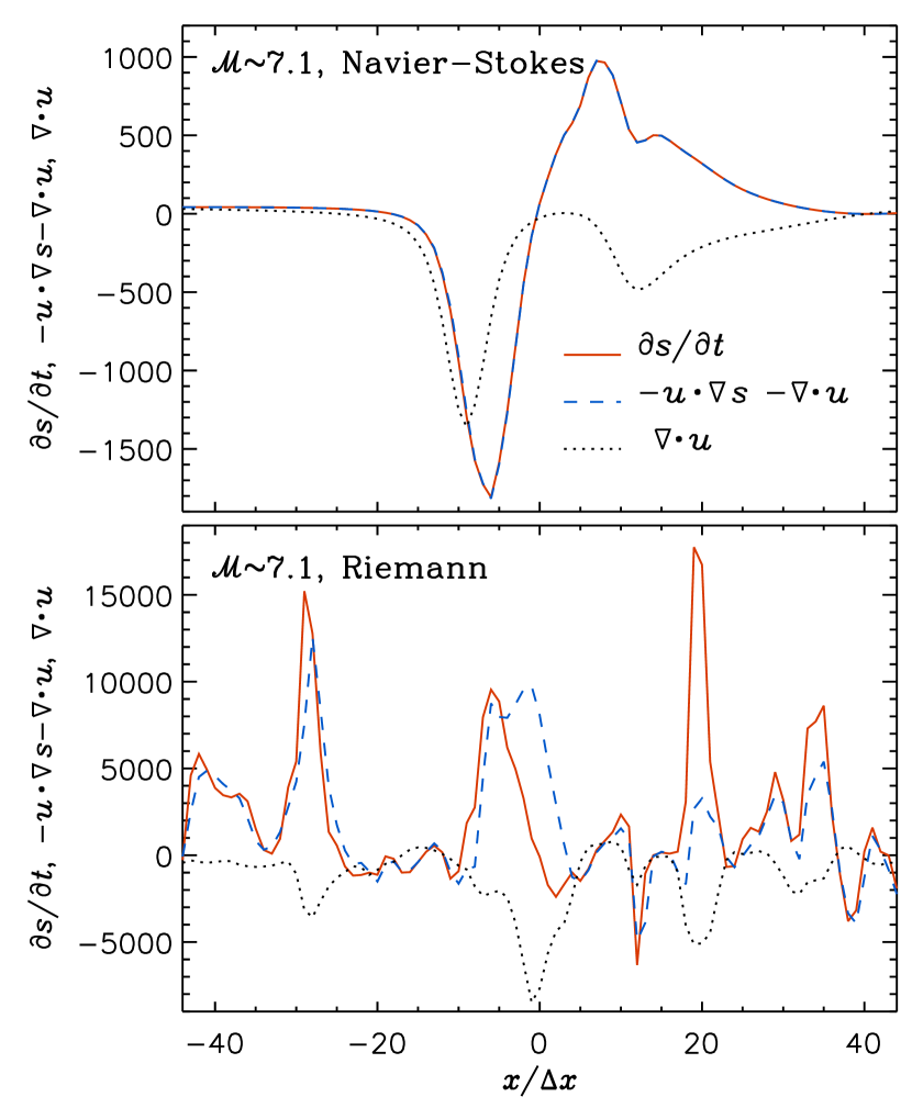
Figure 1.— Test of the continuity equation on a line segment of the simulation grid at an arbitrarily selected snapshot. The chosen line segment is centered around the maximum density (at $x=0$) in the selected snapshot. The distance to the center is in units of the size, $\Delta x$, of the computational cells. The solid, dashed and dotted lines plot $\partial_{t}s$, $-{\boldsymbol{u}}\cdot\nabla s-\nabla\cdot{\boldsymbol{u}}$, and $\nabla\cdot{\boldsymbol{u}}$, respectively, on the line segment. In the N-S run (top panel), the solid and dashed lines coincide, while the disagreement between solid and dashed lines in the Riemann run (bottom panel) indicates the violation of the continuity equation. The snapshots are taken from $1024^{3}$ runs with Mach number $\mathcal{M}=7.1$.

The main goal of the current work is to examine the accuracy of spatial derivatives in numerical simulations of supersonic turbulence. We start with a test against the continuity equation. Figure 1 shows how well the continuity equation is satisfied in 1024³ simulations of supersonic turbulence at Mach 7.1. The solid, dashed and dotted lines plot $\partial_{t}s$, $-{\boldsymbol{u}}\cdot\nabla s-\nabla\cdot{\boldsymbol{u}}$ and $\nabla\cdot{\boldsymbol{u}}$ on a line segment of the simulation grid at an arbitrarily selected snapshot. The line segment is centered around the maximum density in the snapshot. The top and bottom panels correspond to the N-S and Riemann runs, respectively. In the top panel, the solid and dashed lines coincide with each other, demonstrating that the Eq. (3) is well satisfied in the N-S run.

On the other hand, significant discrepancy is seen between the solid and dashed lines in the bottom panel for the Riemann run. The discrepancy appears to correlate with the dips in the dotted line for the flow divergence, $\nabla\cdot{\boldsymbol{u}}$, which correspond to shocks. The disagreement between the solid and dashes lines indicates that the continuity equation is not satisfied, and the problem is most severe around shocks. As pointed out in the Introduction, the spatial derivatives computed from simulations without explicit viscosity are controlled by the numerical algorithm adopted in the code, and may suffer from the artifacts induced by numerical schemes to stabilize the shocks. This is confirmed by the observation that Eq. (3) is strongly violated around shocks.

A comparison of the top and bottom panels of Figure 1 reveals that structures in the N-S run are much smoother than in the Riemann run. The effective resolution or effective Reynolds number in the Riemann runs without explicit viscosity is significantly higher than in the simulations that evolve the N-S equations. This is precisely the motivation for the development of numerical codes based on the Euler equations, which lead to a more extended inertial range than in the simulations including explicit viscosity (Sytine et al. 2000). However, the achievement of significantly higher effective resolution comes with the price of losing accuracy in the spatial derivatives computed from the simulation data. As a consequence, the continuity equation appears to be violated even though mass conservation is strictly enforced in the code.

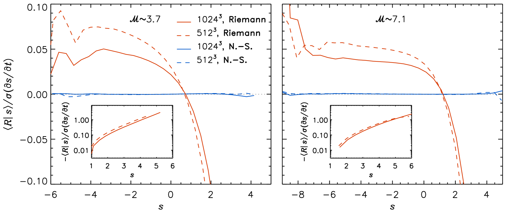
Figure 2.— Conditional average, $\langle R|s\rangle$, of the artificial residual of the continuity equation, normalized to the rms of $\partial_{t}s$ in all the simulated flows. Left and right panels show $\mathcal{M}=3.7$ and $7.1$, respectively. Red and blue correspond to the Riemann and N-S runs, whereas dashed and solid lines correspond to resolutions of $512^{3}$ and $1024^{3}$, respectively. In the Riemann runs, $\langle R|s\rangle$ deviates significantly from zero (black dotted lines). The insets show the normalized residual at large $s$ in the Riemann runs.

3.2. The conditional mean residual $\langle R|s\rangle$

In Figure 2, we show the conditional average, $\langle R|s\rangle$, of the numerical residual of the continuity equation. As discussed in §2, $\langle R|s\rangle$ measures the degree to which the continuity equation is violated in regions at a given density level. All the lines in Figure 2 normalize $\langle R|s\rangle$ to $\langle(\partial_{t}s)^{2}\rangle^{1/2}$, the rms of the rate of change of $s$ in the simulated flows. In both panels, the blue lines, corresponding to the N-S runs, are almost exactly zero at all $s$, demonstrating that the Eq. (3) is nearly perfectly satisfied for both Mach numbers and both numerical resolutions. This is consistent with the top panel of Figure 1, which shows $R\approx 0$ in the N-S runs.

In contrast, the red lines, corresponding to the Riemann runs, show that $\langle R|s\rangle$ deviates significantly from zero at both small and large densities. At intermediate to low densities, the deviation is typically within $\simeq 10$ percent for both Mach numbers. Apparently, at $s\;\hbox to0.0pt{\lower 2.5pt\hbox{$\sim$}\hss}\raise 1.5pt\hbox{$<$}\;0$, $\langle R|s\rangle$ gets closer to 0 as the resolution increases, suggesting that at sufficiently high resolution the continuity equation may be better satisfied in low-density regions.

In the dense regions, the departure of $\langle R|s\rangle$ from zero becomes progressively stronger with increasing $s$. The problem is very severe at the largest values of $s$. The insets plot $\langle R|s\rangle$ at $s\;\hbox to0.0pt{\lower 2.5pt\hbox{$\sim$}\hss}\raise 1.5pt\hbox{$>$}\;1$ with a logarithmic scale, showing that the departure from zero increases almost exponentially with $s$. At the largest density, the normalized residual reaches a value as large as $\simeq 1$, which means that the continuity equation is completely violated. As discussed earlier, whenever numerical techniques are needed to stabilize shocks, numerical errors arise, and, due to the higher probability to encounter shocks, the denser regions are expected to suffer stronger numerical artifacts. This explains why the worst situation occurs at the largest $s$. Furthermore, at large $s$, the dependence of the normalized residual on the numerical resolution appears to be quite weak, especially for the $\mathcal{M}=7.1$ case (see the inset of the right panel). Therefore, the problem at the large densities may not be easily remedied by increasing the numerical resolution.

The departure of $\langle R|s\rangle$ from 0 in the Riemann runs means that at least one of the three terms, i.e., $\langle\partial_{t}s|s\rangle$, $\langle\boldsymbol{u}\cdot\nabla s|s\rangle$, and $\langle\nabla\cdot\boldsymbol{u}|s\rangle$, in Eq. (4) is nonzero. In the following subsections we examine each of the three terms to establish their relative contribution, especially at large $s$.

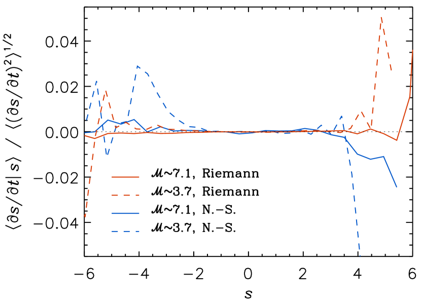
Figure 3.— Conditional mean of the time derivative of $s$, normalized to $\langle(\partial_{t}s)^{2}\rangle^{1/2}$, in $1024^{3}$ simulations. For both Riemann (red line) and N-S (blue line) runs, $\langle\partial_{t}s|s\rangle$ is close to zero (dotted line), with typical deviations of only a few percent.

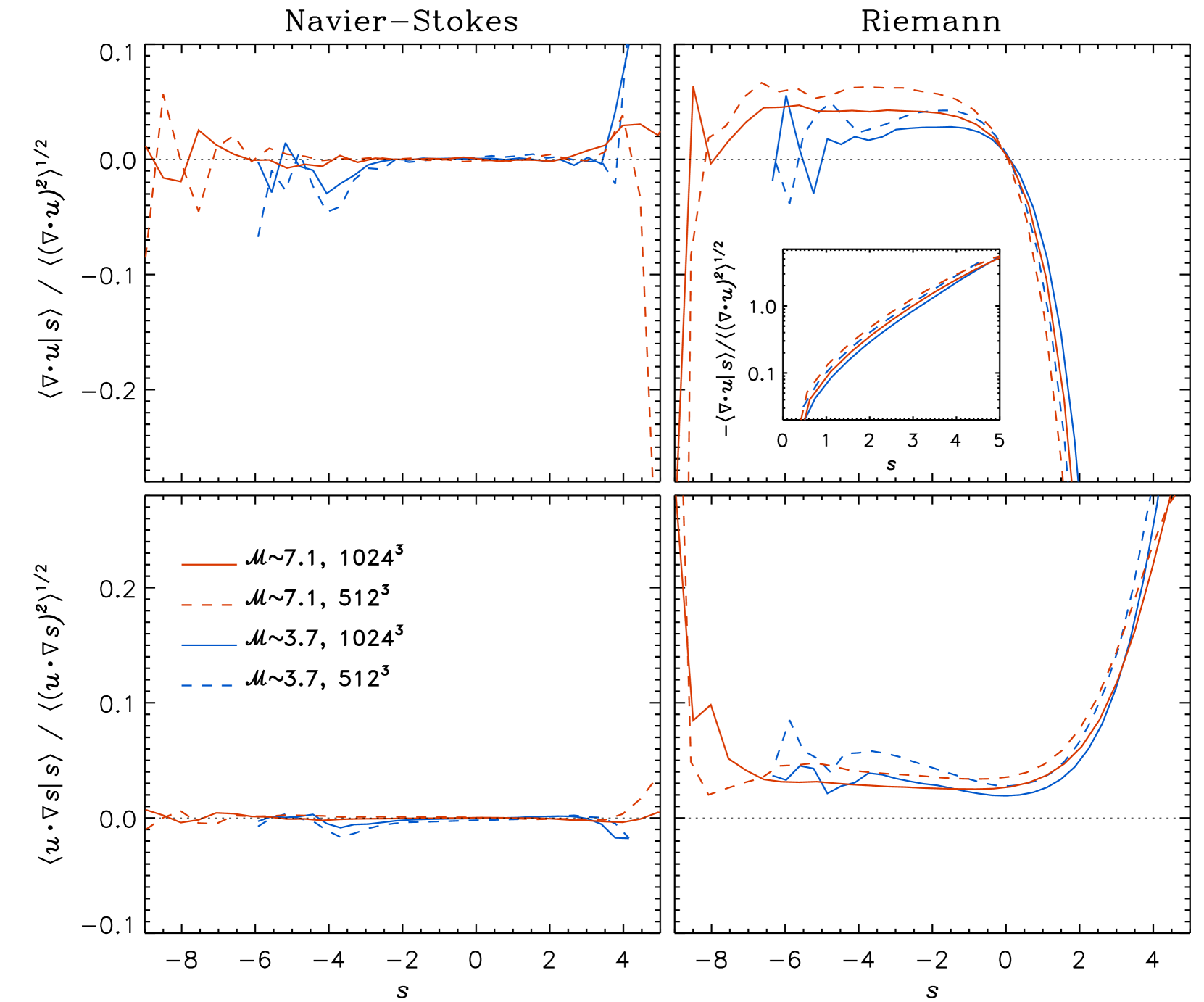
Figure 4.— Conditional mean divergence (top panels) and conditional mean advection (bottom panels) in the N-S (left panels) and Riemann (right panels) runs. Both $\langle\nabla\cdot\boldsymbol{u}|s\rangle$ and $\langle\boldsymbol{u}\cdot\nabla s|s\rangle$ are predicted to be zero (black dotted line) at steady state. The inset in the top right panel shows the large departure of the conditional mean divergence from zero in dense regions.

3.3. The conditional mean of the time derivative of $s$

In §2.1, the conditional mean, $\langle\partial_{t}s|s\rangle$, of the time derivative of $s$ was predicted to be exactly zero once the flow reaches statistically steady state. Figure 3 plots $\langle\partial_{t}s|s\rangle$, normalized to the rms of $\partial_{t}s$ in the $1024^{3}$ runs. It turns out that $\langle\partial_{t}s|s\rangle$ is close to zero in all the simulated flows, with typical deviations less than a few percent. The departure occurs only at extreme values of $s$ where the sample size is smaller, and is thus likely due to insufficient statistics. For a given $s$ bin, the sample size is proportional to the probability distribution function (PDF) of $s$. The sample size at extreme values of $s$, corresponding to the PDF tails, increases with the Mach number $\mathcal{M}$ because the PDF is broader at larger $\mathcal{M}$, and is larger for the Riemann runs where the effective numerical resolution is higher. For the Riemann run at Mach 7.1, the sample size at extreme $s$ is the largest, and this is why the departure of the red solid line from zero is the smallest. On the other hand, the blue dashed line, corresponding to the N-S run at Mach 3.7, shows the largest noise at extreme values of $s$.

The derivation for $\langle\partial_{t}s|s\rangle=0$ in §2.1 relies only on the assumption of steady state, so the finding that $\langle\partial_{t}s|s\rangle$ is close to zero in the simulated flows verifies that the snapshots used in the analysis have already reached steady state. Since $\langle\partial_{t}s|s\rangle=0$ for all flows, the departure of $\langle R|s\rangle$ from 0 found in Figure 2 in the Riemann runs must come from the other two terms, $\langle\nabla\cdot\boldsymbol{u}|s\rangle$ and $\langle\boldsymbol{u}\cdot\nabla s|s\rangle$, in Eq. (4). As these two terms depend on the spatial derivatives, this implies that the spatial derivatives computed from the Riemann runs are inaccurate. This is consistent with the fact that the time derivative of $s$ is the value used to update the solution for $s$, so it cannot be the source of the inaccuracy in the continuity equation (otherwise the solution itself would be inaccurate), while the values of the spatial derivatives derived from cell centered values are not what the HLLC solver uses to update the conserved quantities, and hence there is no a priori reason to expect consistency between such derivatives and the evolution of conserved quantities.

3.4. Exact results of Pan et al. (2018)

The conditional mean divergence, $\langle\nabla\cdot\boldsymbol{u}|s\rangle$, and conditional mean advection, $\langle\boldsymbol{u}\cdot\nabla s|s\rangle$, were predicted by Pan et al. (2018) to be zero at steady state (Eqs. (11) and (12) in §2.2). The top and bottom panels of Figure 3 plot $\langle\nabla\cdot\boldsymbol{u}|s\rangle$ and $\langle\boldsymbol{u}\cdot\nabla s|s\rangle$, normalized to the rms divergence, $\langle(\nabla\cdot\boldsymbol{u})^{2}\rangle^{1/2}$, and the rms advection $\langle(\boldsymbol{u}\cdot\nabla s)^{2}\rangle^{1/2}$, respectively. The left and right panels correspond to the N-S and Riemann runs, respectively.

The prediction of Pan et al. (2018) is confirmed by the data from the N-S runs. In the left panels, we see that $\langle\nabla\cdot\boldsymbol{u}|s\rangle$ and $\langle\boldsymbol{u}\cdot\nabla s|s\rangle$ are close to zero for both Mach numbers and both resolutions. The agreement of the N-S data with the exact result for the conditional mean advection is particularly impressive. As seen in the bottom left panel, the departure of $\langle\boldsymbol{u}\cdot\nabla s|s\rangle$ from 0 is typically within 1% for all values of $s$. For the conditional mean divergence, the deviation from zero occurs only at extreme densities, where it oscillates around zero (see the top left panel). The oscillation appears to be the noise due to insufficient statistics associated with the limited sample size at extreme densities. Overall, the results in the left panels provide strong numerical support for the exact results derived in Pan et al. (2018).

The right panels test the Riemann runs against the exact results. A similar test was conducted in Pan et al. (2018), who attempted to find possible artifacts in simulations of supersonic turbulence due to the numerical diffusion of the density field. Pan et al. (2018) considered Mach 6 flows at different numerical resolutions, and their simulations were carried out using the same Dispatch code framework, in a similar way as the Riemann runs in the current study. The behaviors of the conditional mean divergence and advection shown in the right panels of Figure 4 are similar to those in Figures 1 and 2 of Pan et al. (2018).

In contrast to the N-S runs, both $\langle\nabla\cdot\boldsymbol{u}|s\rangle$ and $\langle\boldsymbol{u}\cdot\nabla s|s\rangle$ in the Riemann runs show strong, systematic deviations from zero, demonstrating that spatial derivatives based on cell centered values in these runs are not consistent with the actual evolution. In the top right panel, we see that $\langle\nabla\cdot\boldsymbol{u}|s\rangle$ is negative at $s\;\hbox to0.0pt{\lower 2.5pt\hbox{$\sim$}\hss}\raise 1.5pt\hbox{$>$}\;0$ and drops very rapidly toward large $s$. The inset shows that at high densities the amplitude of $\langle\nabla\cdot\boldsymbol{u}|s\rangle$ increases almost exponentially with $s$. A likely origin of the negative mean divergence at large densities is that when a strong convergence steepens into a shock, the Riemann solver prevents additional steepening, by effectively introducing viscosity at the cell level, while a calculation without viscosity instead suggests continued convergence of mass into those cells. A similar argument may be applied to explain the rise of $\langle\boldsymbol{u}\cdot\nabla s|s\rangle$ at large $s$ (see the bottom right panel). The advection, $\boldsymbol{u}\cdot\nabla s$, of $s$ is positive across shocks, and sharp density jumps across shocks tend to make $\langle\boldsymbol{u}\cdot\nabla s|s\rangle$ based on cell centered values locally large. Riemann solvers instead computes momentum fluxes across cell interfaces that vary more smoothly across the shock, effectively creating results similar to viscous diffusion of momentum.

In the right bottom panel, the conditional mean advection $\langle\boldsymbol{u}\cdot\nabla s|s\rangle$ is positive at all $s$ and shows a significant rise as $s$ increases above $\simeq 2$. In Pan et al. (2018), the departure of $\langle\boldsymbol{u}\cdot\nabla s|s\rangle$ from zero was interpreted as related to an artificial/numerical diffusion of the density field. A more correct interpretation, in light of the current result, is that it is the actual evolution that reflects an effect similar to artificial/numerical diffusion, and that it is the lack of such diffusion in direct evaluations of $\langle\boldsymbol{u}\cdot\nabla s|s\rangle$ from Riemann solver solutions that produces the systematically positive values.

The interpretation of Pan et al. (2018) essentially assumes that the inaccuracy of the spatial derivatives can be characterized or quantified by some form of numerical diffusion, while a more precise statement is that measures of the inaccuracy of for example Eq. (3) reflect the level of numerical diffusion that would be needed to make the flux evaluations based on cell-centered values agree with the actual evolution.

Note that different Riemann solvers, with different “sharpness” of the solutions at shocks and contact discontinuities exist. The HLL solver, for example, has a term that effectively diffuses both mass, momentum, and total energy across sharp interfaces. This leads to less sharp transitions, which would result in smaller deviations in Eq. (3) than with the (better) HLLC Riemann solver.

Similar to the results of Pan et al. (2018), the departure of the normalized conditional mean divergence and advection from zero in the Riemann runs appears to decrease with increasing resolution for both Mach 3.7 and 7.1 flows. It was speculated in Pan et al. (2018) that $\langle\nabla\cdot\boldsymbol{u}|s\rangle$ and $\langle\boldsymbol{u}\cdot\nabla s|s\rangle$ would approach zero in the limit of infinite resolution. If so, it would be because the volume filling fraction of large discrepancies became on average smaller.

In the Mach 7.1 flows, $\langle\nabla\cdot\boldsymbol{u}|s\rangle$ and $\langle\boldsymbol{u}\cdot\nabla s|s\rangle$ drop and rise abruptly towards the lowest density. One possibility is that the abrupt behaviors at the smallest $s$ may correspond to the numerical challenge of handling the shocks propagating into regions of extremely low density. However, it is not clear whether these strong features are realistic or merely noise due to the small statistical sample at the lowest density. The conditional means, $\langle\nabla\cdot\boldsymbol{u}|s\rangle$ and $\langle\boldsymbol{u}\cdot\nabla s|s\rangle$, are related by Eq. (9) in §2.2. The equation was used in Pan et al. (2018) to connect the behaviors of $\langle\nabla\cdot\boldsymbol{u}|s\rangle$, $\langle\boldsymbol{u}\cdot\nabla s|s\rangle$ and the PDF of $s$. Equation (9) was derived under the assumption of statistical homogeneity only, so it holds in the Riemann runs, even though the spatial derivatives in those runs are inaccurate. Based on Eq. (9), the abrupt drop of $\langle\nabla\cdot\boldsymbol{u}|s\rangle$ toward the smallest $s$ would follow from the fast rise of $\langle\boldsymbol{u}\cdot\nabla s|s\rangle$.

Combing Figures 2, 3 and 4, we see that in the N-S runs, Eq. (3) is satisfied with $\langle R|s\rangle=0$ in the entire range of $s$, and all the three terms in Eq. (4) are zero at steady state, in agreement with the predictions in §2.1 and §2.2. In the Riemann solver runs, however, only $\langle\partial_{t}s|s\rangle$ is close to zero. Both $\langle\nabla\cdot\boldsymbol{u}|s\rangle$, $\langle\boldsymbol{u}\cdot\nabla s|s\rangle$ show departures from zero, especially in the dense regions. Furthermore, these two terms do not add up to zero, so $\langle R|s\rangle$ deviates significantly from zero. In particular, $\langle R|s\rangle$ decreases very fast below zero at large $s$, corresponding to the rapid drop of $\langle\nabla\cdot\boldsymbol{u}|s\rangle$, in the same $s$ range. At large $s$, $\langle\boldsymbol{u}\cdot\nabla s|s\rangle$ shows an opposite trend, but its rise toward large $s$ is not fast enough to compensate the rapid drop of $\langle\nabla\cdot\boldsymbol{u}|s\rangle$.

3.5. The $p\,dV$ work at steady state

We have shown in §2.3 that, in any barotropic turbulent flow, the energy transfer between kinetic and thermal energy by the $p\,dV$ work is symmetric and the average rate of $p\,dV$ work is expected to be zero, once the flow reaches steady state. Figure 5 tests the simulation data against this result. It plots the average rate, $-\langle p\nabla\cdot{\boldsymbol{u}}\rangle$, at which the $p\,dV$ work converts kinetic energy to thermal energy as a function of time. The red and blue lines correspond to the Mach 3.7 and 7.1 flows, and the solid and dot-dashed lines show the N-S and Riemann runs, respectively. The figure shows a time range from 0.4 sound crossing times when all the flows reach steady state to the end of the simulations at 2 sound crossing times. In order to check whether the $p\,dV$ work plays a significant role in the budget of kinetic energy, we normalize it to the dissipation rate of kinetic energy, estimated as $U^{3}/L$ with $U$ and $L$ the 3D rms velocity and the size of the simulation box, respectively. The solid lines in Figure 5 runs are very close to zero, and the amplitude of the oscillations around zero is less than a few percent, meaning that the $p\,dV$ work in the N-S runs does not cause a net transfer between kinetic and thermal energy, fully consistent with the prediction of §2.3.1.

On the other hand, $-\langle p\nabla\cdot{\boldsymbol{u}}\rangle$ in the Riemann runs appears to be positive at all times, suggesting that the energy exchange by the $p\,dV$ work has a preferred direction. This preferential conversion was also seen in Pan & Scannapieco (2010) and Kritsuk et al. (2013). The simulations of Pan & Scannapieco (2010) were run with the Flash code (Fryxell et al. 2000), while the simulation used in Kritsuk et al. (2013) was carried out with the Enzo code (O’Shea et al. 2004). Both codes adopt the piecewise parabolic method (Colella & Woodward 1984). Like the Riemann runs in the current study, none of those previous simulations included an explicit viscous term. Pan & Scannapieco (2010) computed the ratio of the energy conversion rate, $-\langle p\nabla\cdot{\boldsymbol{u}}\rangle$, by $p\,dV$ work to the injection rate of kinetic energy in six simulated flows with the Mach number ranging from 1 to 6, and found that, at steady state, the ratio is in the range from 15% to 30%. Therefore, Pan & Scannapieco (2010) suggested that the $p\,dV$ work provides an extra channel for kinetic energy loss in supersonic turbulence. In the Mach 6 simulation used by Kritsuk et al. (2013), the $p\,dV$ work to energy injection ratio is 26%, based on the values for the average rate of $p\,dV$ work ($-\langle p\nabla\cdot{\boldsymbol{u}}\rangle$=36.5) and energy injection rate ($\epsilon_{0}$ =140) provided in that study. The ratio of the $p\,dV$ work to the energy dissipation rate in our Riemann runs is about 20-30% (see dot-dashed lines in Figure 5), and considering that the energy dissipation rate is in balance with the injection rate at steady state, this ratio is similar to those found in Pan & Scannapieco (2010) and Kritsuk et al. (2013).

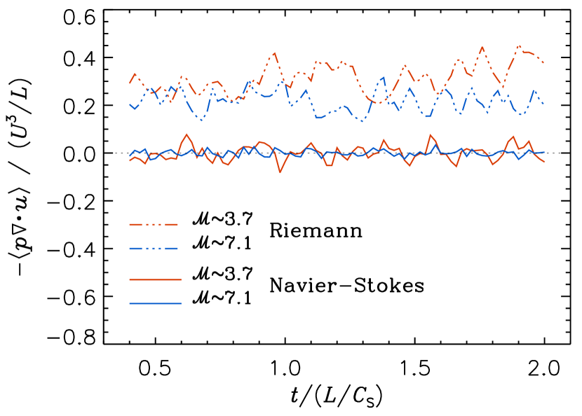
Figure 5.— Average rate of energy conversion from kinetic to thermal energy by $p\,dV$ work in 1024³ runs as a function of time. The time is in units of sound crossing time, while the conversion rate is normalized to the average kinetic energy dissipation rate, estimated as $U^{3}/L$.

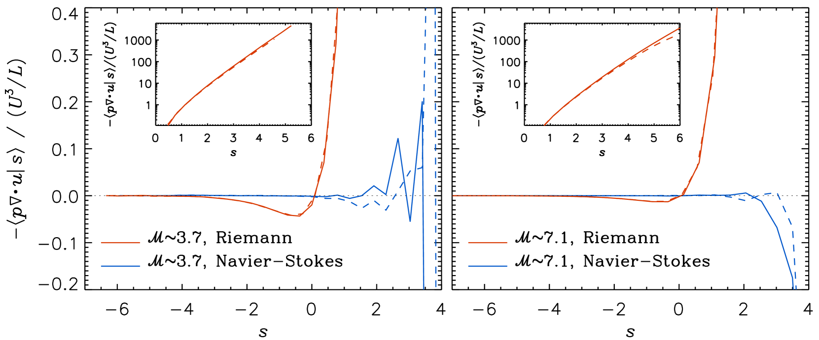
Figure 6.— Conditional mean $p\,dV$ work in Mach 3.7 (left panels) and 7.1 (right panels) flows. Solid and dashed lines correspond to 512³ and $1024^{3}$ runs, respectively. The insets show the sharp rise of the conditional mean $p\,dV$ work in the Riemann runs at $s\;\hbox to0.0pt{\lower 2.5pt\hbox{$\sim$}\hss}\raise 1.5pt\hbox{$>$}\;0.5$. In the N-S runs, departure from 0 occurs only at extremely large values of $s$ where the sample size is small.

The preferential conversion of kinetic energy to thermal energy observed in the simulations that do not include an explicit viscous term are clearly in contraction with our prediction in §2.3 that $\langle p\nabla\cdot{\boldsymbol{u}}\rangle=0$ at steady state for isothermal turbulent flows. One possible interpretation for this contradiction is that the problem is completely caused by the numerical errors in the divergence computed from the data. As shown earlier, spatial derivatives in the Riemann simulations cannot be reliably computed. It could be that the significant, nonzero $p\,dV$ work just reflects the inaccuracy of spatial derivatives, and there is actually no net energy flux from kinetic energy to thermal energy. In other words, the apparent preferential energy conversion is just a false impression due to unreliable divergence computed from the data, and there is nothing wrong with the code except the spatial derivatives. This case is analogous to the test of the continuity equation: Although §3.1 & 3.2 showed that the continuity equation is violated with spatial derivatives computed from the data, it does not indicate that the mass conservation is violated in the simulation.

The second possibility is that the inaccuracy in the spatial derivatives is not fully responsible for the problem, and in the Riemann simulations there is indeed a non-zero energy flux from kinetic energy to effective thermal energy by the $pdV$ work. Unfortunately, this possibility cannot be easily verified or invalidated.

Figure 6 shows the average rate, $-\langle p\nabla\cdot{\boldsymbol{u}}|s\rangle$, of the $p\,dV$ work conditioned on the flow density. In the N-S run (the blue line), the conditional mean is found to be zero at all $s$, except at the largest values $s$ where the statistics is insufficient due to small sample size. This is in agreement with the prediction in §2.3.2 that, at steady state, the $p\,dV$ work in barotropic flows is symmetric at each density level. The prediction $-\langle p\nabla\cdot{\boldsymbol{u}}|s\rangle=0$ simply followed from the fact that the pressure is a function of $s$ only in a barotropic flow and the exact result of Pan et al. (2018) that $\langle\nabla\cdot{\boldsymbol{u}}|s\rangle=0$.

In contrast, the red line from the Riemann solver run shows huge deviations from zero. For isothermal flows, the conditional mean $p\,dV$ work is related to the conditional mean divergence by $-\langle p\nabla\cdot{\boldsymbol{u}}|s\rangle=-C_{\rm s}^{2}\exp(s)\langle\nabla\cdot{\boldsymbol{u}}|s\rangle$. Therefore, the behavior of $-\langle p\nabla\cdot{\boldsymbol{u}}|s\rangle$ follows from that of $\langle\nabla\cdot{\boldsymbol{u}}|s\rangle$ shown in the top right panel of Figure 4. The sharp rise of $-\langle p\nabla\cdot{\boldsymbol{u}}|s\rangle$ above $s\simeq 0$ in the Riemann runs corresponds to the exponential factor and the fast drop of $\langle\nabla\cdot{\boldsymbol{u}}|s\rangle$ at large $s$ (see Figure 4). It is this abrupt rise of $-\langle p\nabla\cdot{\boldsymbol{u}}|s\rangle$ toward large $s$ that gives the main contribution to the significant, positive overall average $p\,dV$ work, $-\langle p\nabla\cdot{\boldsymbol{u}}\rangle$, as observed in Figure 5. The huge, positive conditional mean $p\,dV$ work at large $s$ in the Riemann runs further indicates that the spatial derivatives in the dense regions are highly inaccurate.

In summary, we have found that, consistent with our exact result, the $p\,dV$ work in the N-S runs is symmetric at steady state, causing no energy flux between kinetic and thermal energy. If the Riemann solver solutions are analyzed using cell centered derivatives, a significant non-zero average $p\,dV$ work is observed, which leaves the (incorrect) impression that the $p\,dV$ work in supersonic turbulence preferentially converts kinetic energy to thermal energy.

4. Discussion

We have found that spatial derivatives based on cell-centered values from simulations that evolve the Euler equations cannot be trusted. Previous works based on such simulations that involve spatial derivatives in supersonic turbulence need to be revisited or reinterpreted. For example, the conclusions drawn in previous studies from Euler simulations concerning the $p\,dV$ work in supersonic turbulence are found to be invalid. Kritsuk et al. (2013) attempted to verify the exact result of Galtier & Banerjee (2011) concerning the energy cascade in the inertial range of supersonic turbulence. The exact result is analogous to Kolmogorov’s 4/5 law for incompressible turbulence. But unlike Kolmogorov’s 4/5 law, which only involves the 3rd order velocity structure function, the result of Galtier & Banerjee (2011) includes two terms, a “flux” term that reduces to the 3rd order structure function in the case of incompressible flows, and a “source” term that depends on the divergence. Since the divergence computed from simulations without explicit viscosity is unreliable, based on the discussions on the $p\,dV$ work in §3.5, the evaluation of the source term in Kritsuk et al. (2013) using simulations with a PPM code may suffer from numerical artifact. Thus, the numerical analysis of the exact result of Galtier & Banerjee (2011), in particular the analysis of the source term, should be re-examined using simulations that include explicit viscosity.

In order to understand the kinetic energy cascade in compressive turbulence, Aluie et al. (2012) examined the effects of pressure dilatation using numerical simulations that evolved the Euler equations with a central finite-volume scheme. From the simulation data, they computed the pressure-dilatation cospectrum, $E^{\rm PD}(k)$, defined as $E^{\rm PD}(k)=-\sum\limits_{k-0.5\leq\boldsymbol{k}<k+0.5}p^{*}({\boldsymbol{k}})D({\boldsymbol{k}})$, where $p^{*}({\boldsymbol{k}})$ is the complex conjugate of the Fourier transform of the pressure $p$ and $D({\boldsymbol{k}})$ is the Fourier transform of the velocity divergence, $\nabla\cdot{\boldsymbol{u}}$. The integral of $E^{\rm PD}(k)$ over the $k$ space is equal to $-\langle p\nabla\cdot{\boldsymbol{u}}\rangle$. Aluie et al. (2012) stated that, as $K\to\infty$, the integral $\int_{0}^{K}E^{\rm PD}(k)dk$ converges to a constant, denoted as $\theta$. Clearly, $\theta$ corresponds to $-\langle p\nabla\cdot{\boldsymbol{u}}\rangle$, so it must be zero at steady state in their forced turbulence runs (Runs I & III) with an isothermal equation of state. However, the top panels of their Figure 3 for Runs I & III suggest that $\theta>0$, meaning that the $p\,dV$ work in their simulations also appears to convert kinetic energy to thermal energy. In particular, in their Run III for Mach 1.25, the average rate of the $p\,dV$ work is about 20% of the flux of energy cascade in the inertial range. This is in contradiction to our result in §2.3 that $\theta=-\langle p\nabla\cdot{\boldsymbol{u}}\rangle=0$ at steady state. The likely reason is again that the simulations of Aluie et al. (2012) did not include viscosity, and thus the computation for the divergence is unreliable.

The problem can also be seen from the top panel of their Figure 2 for the cospectrum, $E^{\rm PD}(k)$. Apparently, $E^{\rm PD}(k)$ in their forced runs does not integrate to zero. The cospectrum computed from our simulation data shows that $E^{\rm PD}(k)$ in the N-S runs is qualitatively different from that in the Riemann runs. As seen in our Figure 7, in the Riemann runs, $E^{\rm PD}(k)$ is positive in most $k$ range, and becomes negative only towards the dissipation range. The cospectrum in the Mach 1.45 run of Aluie et al. (2012) shows a similar behavior. In contrast, the cospectrum in the N-S runs oscillates around zero, and its integral is zero as the negative part of the spectrum cancels out the positive part. This suggests that the cospectrum computed by Aluie et al. (2012) suffers from inaccuracies in the divergence evaluated from their simulation, and the effects of pressure dilatation interactions on the kinetic energy budget in compressible turbulence should be reexamined using simulations that include explicit viscosity.

Large differences in $E^{\rm PD}(k)$ between the Riemann and N-S runs are found also in inertial-range wave numbers (Figure 7), suggesting that the inaccurate evaluation of spatial derivatives from solutions of turbulent flows computed without explicit viscosity may even affect inertial-range statistics. One might attribute this qualitative difference in the inertial range solely to the inaccurate divergence in the Riemann runs, and expect that no such problem arises for flow quantities that do not involve gradients. However, we have verified the same problem arises when computing the cospectrum in terms of the Fourier transform, $u_{i}({\boldsymbol{k}})$, of the velocity field as $E_{i}^{\rm PD}(k)=-i\sum\limits_{k-0.5\leq\boldsymbol{k}<k+0.5}k_{i}p^{*}({\boldsymbol{k}})u_{i}({\boldsymbol{k}})$. Therefore, the difference in $E^{\rm PD}(k)$ between the Riemann and N-S runs indicates that the pressure-velocity cospectrum, $\langle p^{*}({\boldsymbol{k}})u_{i}({\boldsymbol{k}})\rangle$ (or equivalently the cross correlation function, $\langle p({\boldsymbol{x}})u_{i}({\boldsymbol{x}}+{\boldsymbol{r}})\rangle$) in the Riemann runs also suffers from numerical artifacts that extend to inertial-range scales. The pressure-velocity cospectrum does not involve any spatial gradients, suggesting the existence of inaccuracies in the post-processing of Euler simulations even when spatial derivatives are not involved. Future work should address the extent to which such inaccuracies affect other inertial-range diagnostics in Euler simulations.

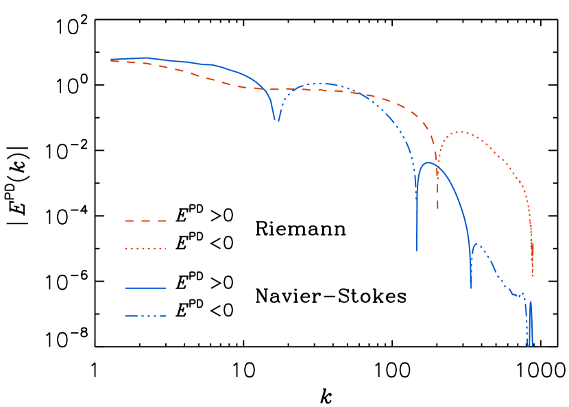
Figure 7.— Pressure-dilatation cospectrum, $E^{\rm PD}(k)$, in the 1024³ simulations for the Mach 7.1 flow. The red and blue lines correspond to the Riemann and N-S runs. In the N-S run, the cospectrum oscillates around zero, and the integration of the cospectrum is zero, with the negative part canceling out the positive part. On the other hand, the cospectrum in the Riemann run does not integrate to zero.

Finally, we point out that the study of the viscous dissipation of kinetic energy in turbulent flows requires an accurate computation of the velocity gradient (e.g. Pan & Padoan 2009, Pan et al. 2009), so the statistics of the dissipation rate in supersonic turbulence should be re-analyzed using simulations that include explicit viscosity. This represents a significant hurdle for such study, because we generally aim at characterizing the viscous dissipation in the limit of very large Reynolds number, which is difficult to achieve with N-S runs.

5. Conclusions

We examined the accuracy of spatial derivatives in numerical simulations of supersonic turbulence. We conducted two sets of simulations using the Dispatch code framework, one based on a finite-volume method to solve the Euler equations and the other based on a finite-difference method to solve the Navier-Stokes equations. We tested them against a number of criteria based on the continuity equation, including some exact results derived from the continuity equation at statistically steady state. We summarize our conclusions as follows:

1. The spatial derivatives based on the N-S runs are accurate and satisfy all the criteria adopted in our study. In particular, the data from N-S runs confirm the exact results derived by Pan et al. (2018), i.e., the conditional mean divergence, $\langle\nabla\cdot{\boldsymbol{u}}|s\rangle$, and the conditional mean advection $\langle{\boldsymbol{u}}\cdot\nabla s|s\rangle$ vanish at statistically steady state.

2. Without an explicit physical viscosity, the structure of discontinuities in the Riemann solver is controlled by numerical schemes involving flow corrections designed to achieve numerical stability. This induces errors in finite-difference derivative expressions, even if the code enforces the conservation laws (in integral form). As a consequence, the Riemann solver runs fail all the tests that require accurate evaluation of spatial derivatives

3. In the Riemann solver runs, the continuity equation appears to be violated with spatial derivatives computed from the data, especially in high-density regions where most shocks inhabit, even though mass conservation is strictly enforced in the code.

4. In the Riemann solver runs, $\langle\nabla\cdot{\boldsymbol{u}}|s\rangle$ and $\langle{\boldsymbol{u}}\cdot\nabla s|s\rangle$ deviate significantly from zero at large densities. These deviations further illustrate the inaccuracy of using cell-centered finite-difference spatial derivatives when post-processing data from simulations that do not include explicit viscosity.

5. We have shown that the energy exchange between kinetic and thermal energy by $p\,dV$ work is symmetric in isothermal, supersonic turbulence once the flow reaches steady state. This analytical result is confirmed by the N-S runs.

6. The inaccuracy of spatial derivatives based on the Riemann solver runs gives the incorrect impression that the $p\,dV$ work tends to preferentially convert kinetic energy to thermal energy. This problem also exists in the interpretation of previous simulations using other numerical codes, indicating that the unreliability of cell-centered spatial derivatives is a general issue for all simulations that do not include explicit viscosity. Furthermore, we found that the pressure-dilatation cospectrum in the N-S and Riemann runs shows large qualitative differences also at inertial-range scales.

Our work suggests that studies involving spatial gradients in supersonic turbulence must be carried out and interpreted with caution. In principle, one may need to include explicit viscosity in the simulation in order to obtain accurate spatial derivatives in post-processing analyses. The extent to which diagnostics of inertial-range dynamics are also affected, as in the example of the pressure-dilation cospectrum reported here, will be further investigated in future studies.

References

- Aluie et al. (2012) Aluie, H., Li, S. & Li, H. 2012, ApJ, 751, L29
- Baumann et al. (2012) Baumann G., Galsgaard K., Nordlund A. 2013, Solar Physics 284, 467
- Colella & Woodward (1984) Colella, P., & Woodward, P. R. 1984, Journal of Computational Physics, 54, 174
- Frisch (1995) Frisch, U. 1995, Turbulence: The legacy of A. N. Kolmogorov, Cambridge, UK: Cambridge University Press
- Fryxell et al. (2000) Fryxell, B., Olson, K., Ricker, P., et al. 2000, ApJS, 131, 273
- Galsgaard & Nordlund (1996) Galsgaard K., Nordlund Å. 1996, Journal of Geophysical Research 101, 13445
- Galtier & Banerjee (2011) Galtier, S. & Banerjee, S., 2013, Phys. Rev. Lett. 107 (13), 134501
- Kida & Orszag (1990) Kida, S., & Orszag, S. A. 1990, J. Sci. Comput., 5, 85
- Kida & Orszag (1992) Kida, S., & Orszag, S. A. 1992, J. Sci. Comput., 7, 1
- Kritsuk et al. (2007) Kritsuk, A. G., Norman, M. L., Padoan, P., & Wagner, R. 2007, ApJ, 665, 416
- Kritsuk et al. (2011) Kritsuk, A. G., Nordlund, Å., Collins, D., et al. 2011, ApJ, 737, 13
- Kritsuk et al. (2013) Kritsuk, A. G., Wagner, R., & Norman, M. L. 2013, Journal of Fluid Mechanics, 729, R1
- Nordlund et al. (2018) Nordlund, Å, Ramsey, J. P., Popovas, A., & Küffmeier, M. 2018, MNRAS, 477, 624
- O’Shea et al. (2004) O’Shea, B. W., Bryan, G., Bordner, J., et al. 2004, arXiv:astro-ph/0403044
- Padoan et al. (2014) Padoan, P., Federrath, C., Chabrier, G., et al. 2014, Protostars and Planets VI, 77
- Pan & Padoan (2009) Pan, L. & Padoan, P. 2009, ApJ, 692, 594
- Pan et al (2009) Pan, L., Padoan, P., & Kritsuk, A. G. 2009, Phys. Rev. Lett., 102, 034501
- Pan et al. (2018) Pan, L., Padoan, P., & Nordlund, Å. 2018, ApJ, 866, L17
- Pan & Scannapieco (2010) Pan, L. & Scannapieco, E. 2010, ApJ, 721, 1765
- Pavlovski et al. (2006) Pavlovski, G., Smith, M. D., Mac Low, M.-M. 2006, MNRAS, 368, 943
- Pope (2000) Pope, S. B. 2000, Turbulent Flows, by Stephen B. Pope, pp. 806. ISBN 0521591252. Cambridge, UK: Cambridge University Press, September 2000., 806
- Porter et al. (1992) Porter, D. H., Pouquet, A., & Woodward, P. R. 1992a, Phys. Rev. Lett., 68, 3156
- Porter et al. (1992) Porter, D. H., Pouquet, A., & Woodward, P. R. 1992b, Theoret. Comput. Fluid Dynamics, 4,13
- Porter et al. (1998) Porter, D. H., Woodward, P. R., & Pouquet, A. 1998, Phys. Fluids, 10, 237
- Porter et al. (2002) Porter, D. H., Woodward, P. R., & Pouquet, A. 2002, Phys. Rev. E, 66, 026301
- Sytine et al. (2000) Sytine, I. V., Porter, D. H., Woodward, P. R., Hodson, S. W. & Winkler, K.-H. 2000, Journal of Computational Physics,158, 225
- Sur et al. (2014) Sur, S., Pan, L. & Scannapieco, E. 2014, ApJL, 790, L9
- Toro et al. (1994) Toro, E. F., Spruce, M. & Speares, W. 1994, Shock Waves, 4, 25
- Vazquez-Semadeni (1994) Vazquez-Semadeni, E. 1994, ApJ, 423, 681
- Wang et al. (2012) Wang, J., Shi, Y., Wang, L.-P., et al. 2012, Physical Review Letters, 108, 214505