Abstract

We discuss the particle horizon problem in the framework of spatially homogeneous and isotropic scalar cosmologies. To this purpose we consider a Friedmann–Lemaître–Robertson–Walker (FLRW) spacetime with possibly non-zero spatial sectional curvature (and arbitrary dimension), and assume that the content of the universe is a family of perfect fluids, plus a scalar field that can be a quintessence or a phantom (depending on the sign of the kinetic part in its action functional). We show that the occurrence of a particle horizon is unavoidable if the field is a quintessence, the spatial curvature is non-positive and the usual energy conditions are fulfilled by the perfect fluids. As a partial converse, we present three solvable models where a phantom is present in addition to a perfect fluid, and no particle horizon appears.

xx 1 5 yes On the Necessity of Phantom Fields for Solving the Horizon Problem in Scalar Cosmologies Davide Fermi ^1,2,*^,†, Massimo Gengo ^1,† and Livio Pizzocchero ^1,2,† Davide Fermi, Livio Pizzocchero Correspondence: davide.fermi@unimi.it These authors contributed equally to this work. 98.80.-k; 98.80.Cq; 95.36.+x; 04.40.Nr 83-XX; 83F05; 83C15

1 Introduction

There are many reasons for considering cosmological models where a classical scalar field is present, in addition to ordinary matter and radiation.

Since the beginning of 1980s, it was suggested that a scalar field could be related the alleged inflationary behavior of the early universe Guth (1981); Linde (1982, 1983); Madsen (1988). The subsequent literature is too wide for an exhaustive account, thus we limit ourselves to mentioning Barrow (1990); Coley (2003); Guth (2000); Linde (1990, 2004); Lucchin (1985); Olive (1990).

In the late 1980s, a scalar field was proposed as a simple, but nontrivial dynamical model for dark energy Ratra (1988). The presence of some kind of dark energy was just a possible scenario in this seminal work, but became a consolidated idea after the experimental discovery of the present time accelerated expansion of the universe Perlmutter (1999); Riess (1998). Even the literature on scalar models of dark energy is enormous; here we only cite Caldwell (1998); Elizalde (2004); Matos (2000); Piedipalumbo (2012); Sahni (2000); Saini (2000); Sola (2017).

Starting from the above physical motivations, many authors focused the attention on the mathematically rigorous treatment of cosmological models with scalar fields. Exact solutions of the Einstein equations for these models are obtained in Barrow (1987); Burd (1988); Cataldo (2013); Chimento (1998); Gengo (2019); deRitis (1990, 1991); Easther (1993); Fre (2013); Ratra (1988); Paliathanasis (2014, 2015); Piedipalumbo (2012); Rubano (2002). Again, in the area of exact solutions, we would mention a peculiar, “inverse” approach to the evolution equations of scalar cosmologies: here the time dependence of the scale factor (or of some other physically relevant quantity) is prescribed, and the Einstein equations are used to determine the other observables of the model, including the self-interaction potential of the scalar field Barrow (1990, 2016); Ellis (1991); Lucchin (1985).

Up to now, we have generically employed the term “scalar field” to indicate either a canonical field (also called a quintessence in cosmology), or a phantom field, with an anomalous sign in the kinetic part of the action functional.

Phantom fields were originally introduced in cosmology as toy models in which the equation of state parameter (i.e., the ratio of the pressure to the density) can attain values below $-1$ Caldwell (2002); Carroll (2003); it is perhaps superfluous to recall that such a behavior implies a violation of the weak energy condition Hawking (1975). It is well known that the (renormalized) vacuum expectation value of the stress–energy tensor of a quantized canonical field (see, e.g., Bytsenko (2003); Fermi (2017)) also violates this energy condition; thus, phantom fields can be viewed as simplified models for quantum vacua of canonical fields, as first remarked in Nojiri (2003).

In applications to cosmology, phantom fields were mainly considered in connection with the present day accelerated expansion Caldwell (2002); Capozziello (2006); Carroll (2003); Dutta (2016); Elizalde (2004); Gibbons (2003); Singh (2003). The aim of the present work is to provide a different motivation to focus the attention on phantoms, connected with the early history of universe. The subject that we wish to link to phantom fields is the well known horizon problem, which can be described as follows for any Friedmann–Lemaître–Robertson–Walker (FLRW) cosmology Ellis (1988); Hawking (1975); Plebanski (2006); Rindler (1956); Wald (1984). Depending on the behavior of the scale factor close to the Big Bang, at a given instant, there are two alternatives for any particle at rest in the FLRW frame: the spatial region that has already interacted with the particle either is confined within a suitable horizon, or is the whole space (no particle horizon). Of course, the absence of a horizon is the physically most pleasant case: in fact, due to the causal connection of the whole space to any point, we can invoke some kind of thermalization process to explain the homogeneity of the universe.

In this paper, we discuss the horizon problem for FLRW cosmologies with a scalar field and a finite number of perfect fluids, each of them representing some (reasonable) kind of matter or radiation. Here are the main outputs of this analysis:

1. Putting the usual energy conditions on the state equations of the fluids and assuming a non-positive spatial curvature, we prove that a quintessence (canonical scalar field) with an arbitrary self-interaction potential always produces a particle horizon. This fact was probably noticed in specific cases but, to the best of our knowledge, it was never proved with the present generality. The conditions on the state equations of the fluids that we assume are satisfied, e.g., by dust and by a radiation gas. Our requirement of non-positive curvature is, mainly, to simplify the analysis; we hope to discuss elsewhere the case of positive curvature, using arguments similar to the present ones.

2. In view of (I), the quest for scalar cosmologies with (non-positive curvature and) no particle horizon naturally brings us to consider the phantom case. We show that a phantom field with a suitable self-potential, in presence of some reasonable kind of perfect fluid, can indeed produce a FLRW cosmology with no horizon: three examples of this kind are presented. In the first example, we have a spatially flat de Sitter universe (with a Big Bang at an infinitely remote instant); the perfect fluid has a quite arbitrary equation of state, and the phantom field has a quadratic self-interaction potential. In the second example, the spatial curvature is negative, the Big Bang occurs at a finite time, the perfect fluid is a radiation gas and the phantom has a quartic, self-interaction potential of Higgs type. In the third example, the spatial curvature is zero, the Big Bang happens at a finite time, a radiation gas is present and the phantom has an ad hoc self-potential, not expressible via elementary functions. All these examples present an accelerated expansion, and an exponential divergence of the scale factor over long times.

Concerning Item (II), we are aware that phantom fields are potentially responsible for a number of pathological features, such as a Big Rip (the simultaneous divergence of the scale factor, and of the density and pressure at a finite time after the Big Bang) or a Little Rip (divergence of the same quantities in the infinitely far future) Bamba (2012); Brevik (2011); Caldwell (2003); Frampton (2011, 2012); Nojiri (2005); on top of that, it was pointed out that the thermodynamics of phantom fields may cause the appearance of negative temperatures or of a negative total entropy for the universe Brevik (2004); Gonzales (2004); Myung (2009); Nojiri (2004, 2005). Discussing these issues is beyond the purposes of the present work; here, we are led to consider a phantom by purely logical arguments related to Proposition 4, which are inescapable if one wants a cosmological model with no horizon and matter fulfilling the usual energy conditions. In any case, in the examples of this paper the phantom field never produces a Big Rip nor a Little Rip.

Let us briefly illustrate the organization of the paper. Most of the paper refers to a spacetime of arbitrary dimension $d+1$, where $d\geqslant 2$; of course, $d=3$ is the most physically relevant case. Sections 2 and 3 review some basic facts on gravitation in presence of scalar fields and perfect fluids, and on FLRW cosmologies based on the same actors (including the related energy conditions); the horizon problem is summarized in Section 3.1. The aim of these sections is to fix some standards, and to present the Einstein (and Klein–Gordon) equations in a form convenient for our subsequent considerations. Section 4 treats the subject indicated in the previous Item (I), i.e., the fact that a canonical scalar field always produces a particle horizon (in the case of non-positive spatial curvature, and with minimal assumptions on the perfect fluids); the general formulation of this result is contained in Proposition 4. Section 5 has the content described in the previous Item (II), i.e., it presents three cosmologies with a phantom field, a perfect fluid and no particle horizon; these are described in Sections 5.1–5.3, respectively.

A final remark. One of the Reviewers of this paper pointed out that a simpler solution of the horizon problem, avoiding the use of phantom fields, would be to consider a universe filled with a canonical scalar field violating the strong energy condition, at least in an initial interval. However, the aim of this paper is to discuss the horizon problem in a framework where the content of the universe includes some type of ordinary matter, fulfilling the usual energy conditions; according to our Proposition 4, it is just the joint presence of such ordinary matter and of a canonical scalar field that produces a particle horizon. This is the reason, besides ordinary matter, we are led to consider a phantom field.

2 Generalities on Gravity, Perfect Fluids and Scalar Fields

Throughout the paper, we work in natural units, in which the speed of light and the reduced Planck constant are $c=1$ and $\hbar=1$.

As a starting point, let us consider a general model living in a $(d+1)$-dimensional spacetime, of spatial dimension $d\geqslant 2$. Let $x=(x^{\mu})_{\mu=0,...,d}$ be any set of spacetime coordinates. The metric $g_{\mu\nu}$ has signature $(-,+,...,+)$; the corresponding covariant derivative, Ricci tensor and scalar curvature are indicated, respectively, with $\nabla_{\!\mu}$ , $R_{\mu\nu}$ and $R$. We assume the model to include the following:

• $n\geqslant 1$ species of non-interacting perfect fluids, all with the same $(d+1)$-velocity. For any $i\in\{1,...,n\}$, we suppose that the mass-energy density $\rho_{i}$ and the pressure $p_{i}$ of the $i$th fluid are related by a barotropic equation of state of the form $p_{i}=p_{i}(\rho_{i})$.

• A real classical scalar field $\phi$, minimally coupled to gravity and self-interacting with potential $V(\phi)$.

The action functional governing the dynamics of the system outlined above is

$$\SS\,:=\int d^{d+1}\!x\;\sqrt{-g}\left[{R\over 2\kappa_{d}}-\sum_{i=1}^{n}\rho_{i}-{\sigma\over 2}\,g^{\mu\nu}\partial_{\mu}\phi\,\partial_{\nu}\phi-V(\phi)\right],$$ (1)

where $g$ denotes the determinant of the metric $g_{\mu\nu}$ and $\kappa_{d}$ is the Einstein gravitational constant in $d+1$ dimensions. Here and in the sequel, $\sigma$ is a pure sign parameter: in compliance with the standard nomenclature, we call the field $\phi$ a quintessence if $\sigma=+1$ and a phantom if $\sigma=-1$.

The evolution equations for the model can be derived requiring the action $\SS$ to be stationary under variations of the metric, of the fluids’ histories and of the field.

Firstly, the stationarity condition for variations of the metric $g_{\mu\nu}$ yields the Einstein equations

$$R_{\mu\nu}-{1\over 2}\,R\,g_{\mu\nu}=\kappa_{d}\left(\,\sum_{i=1}^{n}T^{i}_{\mu\nu}+T^{\phi}_{\mu\nu}\right);$$ (2)

these involve the stress–energy tensors of the fluids and of the field, defined, respectively, as

$$T^{i}_{\mu\nu}:=(p_{i}+\rho_{i})\,U_{\mu}\,U_{\nu}+\,p_{i}\,g_{\mu\nu}\quad\;\mbox{for\; $i\in\{1,...,n\}$}\,,$$ (3)

$$T^{\phi}_{\mu\nu}:=\sigma\!\left(\partial_{\mu}\phi\,\partial_{\nu}\phi-{1\over 2}\,g_{\mu\nu}\,\partial^{\gamma}\phi\,\partial_{\gamma}\phi\right)-V(\phi)\,g_{\mu\nu}\,,$$ (4)

with $U^{\mu}$ indicating the common $(d+1)$-velocity vector field of all the fluids.

Secondly, stationarity of $\SS$ under variations of the fluids’ histories (defined as in (Hawking (1975), Section 3.3)) leads to the separate conservation laws

$$\nabla^{\mu\,}T^{i}_{\mu\nu}=0\quad\;\mbox{for\; $i\in\{1,...,n\}$}\,;$$ (5)

taking this into account and using the contracted Bianchi identity for the Einstein equations (2), we also obtain the analogous conservation law

$$\nabla^{\mu\,}T^{\phi}_{\mu\nu}=0\,.$$ (6)

Lastly, the stationarity condition for $\SS$ with respect to variations of the field $\phi$ gives rise to the Klein–Gordon equation

$$-\,\sigma\,\nabla_{\!\mu}\nabla^{\mu}\phi+V^{\prime}(\phi)=0\,.$$ (7)

As well known, in the phantom case $\sigma=-1$, the evolution equation (7) implies an exotic behavior of the field $\phi$, which spontaneously evolves towards maxima (rather than minima) of the potential $V(\phi)$.

On the other hand, notice that from Equation (4) it follows $\nabla^{\mu\,}T^{\phi}_{\mu\nu}=(\sigma\nabla_{\!\mu}\nabla^{\mu}\phi-V^{\prime}(\phi))\,\partial_{\nu}\phi$, for both $\sigma=+1$ and $\sigma=-1$; thus, whenever $\partial_{\nu}\phi\neq 0$, the conservation law (6) and the field equation (7) are indeed equivalent. We have already noted that the Einstein equations (2) and the conservation laws (5) for the matter fluids imply Equation (6), thus they also convey the Klein–Gordon equation (7) whenever $\partial_{\nu}\phi\neq 0$.

3 The Reference Cosmological Model

The general framework of the previous section can be used to set up a cosmological model, where the perfect fluids are meant to provide an effective description of different types of matter or radiation; here, the scalar field models dark energy over long times, and possibly triggers an initial inflationary behavior.

As customary, we construct a spatially homogeneous and isotropic model. Accordingly, we consider a $(d+1)$-dimensional FLRW spacetime ($d\geqslant 2$), which is the product of a time interval with its natural coordinate $\tau$ (the “cosmic time”) and of a $d$-dimensional complete, simply connected Riemannian manifold $\mathscr{M}_{k}$ (the “space”), of constant sectional curvature $k$ (i.e, a flat Euclidean space if $k=0$, a hyperbolic space if $k<0$ and a spherical surface if $k>0$); we write $d\ell^{2}_{k}$ for the line element of $\mathscr{M}_{k}$ and often refer to $k$ as to the “spatial curvature”. The spacetime line element is

$$ds^{2}=-\,d\tau^{2}\!+a(\tau)^{2}\,d\ell_{k}^{2}\,,$$ (8)

where $a(\tau)>0$ is the dimensionless scale factor.

Concerning the $n$ species of perfect fluids, for any $i\in\{1,...,n\}$, we postulate the linear equation of state

$$p_{i}=w_{i}\,\rho_{i}\,,\qquad\mbox{with constant $w_{i}\in\mathbb{R}$}\,.$$ (9)

Besides, we assume these fluids to be co-moving with the FLRW frame, so that the $(d+1)$-velocity $U^{\mu}$ appearing in the stress–energy tensors in Equation (3) coincides with the coordinate vector field $\partial_{\tau}$. In agreement with the homogeneity hypothesis, we further suppose that their mass–energy densities and pressures depend only on cosmic time, i.e.,

$$\rho_{i}\equiv\rho_{i}(\tau)\,,\qquad p_{i}\equiv p_{i}(\tau)\,.$$ (10)

On account of the assumptions stated above, the conservation equations (5) reduce to

$$\dot{\rho}_{i}+d\,(1+w_{i})\,{\dot{a}\over a}\,\rho_{i}=0\quad\;\mbox{for\; $i\in\{1,...,n\}$}$$ (11)

(here and in the sequel, dots denote derivatives with respect to $\tau$; e.g., $\dot{a}\equiv da/d\tau$). The differential equations (11) are solved by the redshift relations

$$\rho_{i}(\tau)={d\,(d-1)\over 2\,\kappa_{d}}\;{\lambda_{i}\over a(\tau)^{d(1+w_{i})}}\;,$$ (12)

where $\lambda_{i}$ is a constant. The factor $d(d\!-\!1)/(2\kappa_{d})$ has been introduced in Equation (12) for future convenience; note that $d(d\!-\!1)\lambda_{i}/(2\kappa_{d})$ is the density of the $i$th fluid at the instant when the scale factor is $a(\tau)=1$ .

Next, let us consider the field $\phi$; to comply with the homogeneity hypothesis, we assume that also $\phi$ only depends on cosmic time, i.e.,

$$\phi\equiv\phi(\tau)\,.$$ (13)

In this case, the stress–energy tensor (4) is also of perfect fluid form

$$T^{\phi}_{\mu\nu}\!=(p_{\phi}+\rho_{\phi})\,U_{\mu}\,U_{\nu}+p_{\phi}\,g_{\mu\nu}\,,$$ (14)

with density $\rho_{\phi}$ and pressure $p_{\phi}$, respectively, given by

$$\rho_{\phi}:={\sigma\over 2}\,\dot{\phi}^{2}+V(\phi)\,,\qquad p_{\phi}:={\sigma\over 2}\,\dot{\phi}^{2}-V(\phi)\,.$$ (15)

The equation of state parameter for the scalar field can be defined as follows, whenever  $\rho_{\phi}\neq 0$:

$$w_{\phi}:={p_{\phi}\over\rho_{\phi}}={\sigma\,(\dot{\phi}^{2}\!/2)-V(\phi)\over\sigma\,(\dot{\phi}^{2}\!/2)+V(\phi)}\,.$$ (16)

Note that $w_{\phi}$ depends on time (with a law determined by the solution of the cosmological model), while the analogous parameters $w_{i}$ ($i\in\{1,...,n\}$) of the perfect fluids mentioned before are universal constants; this is a good reason to distinguish between any of these $n$ fluids and the scalar field.

Taking into account all the facts mentioned above, the Einstein equations (2)  become 

$${d\,(d-1)\over 2}\left({\dot{a}^{2}\over a^{2}}+{k\over a^{2}}-\sum_{i=1}^{n}{\lambda_{i}\over a^{d(1+w_{i})}}\right)-\kappa_{d}\Bigg{(}{\sigma\over 2}\,\dot{\phi}^{2}+V(\phi)\!\Bigg{)}=\,0\,,$$ (17)

$$(d-1)\!\left({\ddot{a}\over a}+{d-2\over 2}\,{\dot{a}^{2}\over a^{2}}+{d-2\over 2}\,{k\over a^{2}}+{d\over 2}\sum_{i=1}^{n}{w_{i}\,\lambda_{i}\over a^{d(1+w_{i})}}\right)+\kappa_{d}\Bigg{(}{\sigma\over 2}\,\dot{\phi}^{2}-V(\phi)\!\Bigg{)}=\,0\,.$$ (18)

To proceed, let us remark that, in the present framework, the Klein–Gordon equation (7) reduces to

$$\ddot{\phi}+d\,{\dot{a}\over a}\,\dot{\phi}+\sigma\,V^{\prime}(\phi)=0\,.$$ (19)

We already mentioned at the end of Section 2 that, for the general models described therein, the Klein–Gordon equation is indeed a consequence of the Einstein equations whenever the scalar field has non-zero gradient. In the present homogeneous and isotropic framework, this fact can be ascribed to the identity

$${d\over d\tau}\Big{[}a^{d}\cdot\eqref{E1}\Big{]}-d\,a^{d-1}\,\dot{a}\cdot\eqref{E2}+\sigma\,\kappa_{d}\,a^{d}\,\dot{\phi}\cdot\eqref{ffeq}\,=\,0\;,$$ (20)

where the notations (17)–(19) stand for the left-hand sides of Equations (17)–(19); this makes patent that the Einstein equations (17) and (18) imply the Klein–Gordon equation (19) at all times $\tau$ such that $\dot{\phi}(\tau)\neq 0$ .

For later reference, let us point out that Equations (17) and (18) are equivalent to the pair

$$\dot{\phi}^{2}=\,\sigma\,{d-1\over\kappa_{d}}\left[{\dot{a}^{2}\over a^{2}}-{\ddot{a}\over a}+{k\over a^{2}}-{d\over 2}\sum_{i=1}^{n}{(1+w_{i})\,\lambda_{i}\over a^{d(1+w_{i})}}\right],$$ (21)

$$V(\phi)\,=\,{d-1\over 2\,\kappa_{d}}\left[(d-1)\,{\dot{a}^{2}\over a^{2}}+{\ddot{a}\over a}+(d-1)\,{k\over a^{2}}-{d\over 2}\sum_{i=1}^{n}{(1-w_{i})\,\lambda_{i}\over a^{d(1+w_{i})}}\right].$$ (22)

Let us conclude this subsection with two remarks:

1. There are solutions of Equations (17)–(19) with $\phi(\tau)=$ const.​ $\equiv\phi_{\star}$; in particular, Equation (19) shows that a solution of this kind is possible if and only if $V^{\prime}(\phi_{\star})=0$. On the other hand, from Equations (15) and (16) we infer that a function $\tau\to\phi(\tau)$ has a constant value $\phi_{\star}$ if and only if $p_{\phi}=-\rho_{\phi}$, i.e.,​ (assuming $\rho_{\phi}\neq 0$), $w_{\phi}=-1$ at all times. If this occurs, Equation (14) for the field stress–energy tensor gives $T^{\phi}_{\mu\nu}=-\,V(\phi_{\star})\,g_{\mu\nu}$; this is the stress–energy tensor corresponding to a cosmological constant term in the Einstein equations, thus the scalar field is said to behave as a cosmological constant.

2. For future reference, it is convenient to review some known facts about the standard energy conditions (see Hawking (1975) for the usual formulation in spatial dimension $d=3$ and Maeda (2018) for its extension to arbitrary $d\in\{2,3,4,...\}$). Let us fix $i\in\{1,...,n\}$ and consider the $i$th fluid of the previously mentioned family; its stress–energy tensor $T^{i}_{\mu\nu}$ (see Equation (3)) fulfils the weak energy condition if and only if $\rho_{i}\geqslant 0$ and $p_{i}+\rho_{i}\geqslant 0$, while it fulfills the strong energy condition if $p_{i}+\rho_{i}\geqslant 0$ and $d\,p_{i}+(d-2)\,\rho_{i}\geqslant 0$. With the assumption $\rho_{i}>0$ (positive density), the weak and strong energy conditions are, respectively, equivalent to the relations

   $$w_{i}\geqslant-1\,,$$ (23)

   $$w_{i}\geqslant{2\over d}-1\,.$$ (24)

   Of course, one can make similar statements for the scalar field replacing $\rho_{i},p_{i},w_{i}$ with $\rho_{\phi},p_{\phi},w_{\phi}$.

3.1 The Particle Horizon Problem

The subject of the present subsection is relevant for any cosmological model based on a spacetime of the FLRW type, described by Equation (8) and by the related comments. Given any such model, we assume the following:

1. The cosmic time $\tau$ ranges in an interval $(\tau_{0},\tau_{1})$, where $-\infty\leqslant\tau_{0}<\tau_{1}\leqslant+\infty$; besides, the scale factor $\tau\mapsto a(\tau)>0$ is smooth on this interval.

2. A Big Bang occurs at $\tau_{0}$, meaning that

   $$a(\tau)\to 0\quad\mbox{for\; $\tau\to\tau_{0}$}\,.$$ (25)

Correspondingly, let us consider the lapse of conformal time that has passed from the Big Bang up to any cosmic time $\tau\in(\tau_{0},\tau_{1})$, namely,

$$\Theta(\tau):=\!\int_{\tau_{0}}^{\tau}{d\tau^{\prime}\over a(\tau^{\prime})}\,\in\,(0,+\infty]\,.$$ (26)

In our units with $c=1$, $\Theta(\tau)$ represents the distance in $\mathscr{M}_{k}$ (with respect to the metric $d\ell^{2}_{k}$) travelled until cosmic time $\tau$ by a light signal emitted at the Big Bang and propagating freely. On account of this, given any co-moving FLRW particle with position x in $\mathscr{M}_{k}$, the co-moving particles that had enough time to interact causally with it before time $\tau$ are those with position in the ball of $\mathscr{M}_{k}$ with center in x and radius $\Theta(\tau)$, which we denote with $\mathscr{B}(\textbf{x},\Theta(\tau))$. If this ball is smaller than the whole space $\mathscr{M}_{k}$, it has a boundary $\partial\mathscr{B}(\textbf{x},\Theta(\tau))$, which is referred to as the particle horizon of x at cosmic time $\tau$ Ellis (1988); Hawking (1975); Plebanski (2006); Rindler (1956); Wald (1984).

Next, let us notice that, for any $\textbf{x}\in\mathscr{M}_{k}$, the sup of the distances between x and the other points of $\mathscr{M}_{k}$ is independent of x and equals

$$\delta_{k}:=\left\{\!\!\begin{array}[]{ll}\displaystyle{\infty}&\displaystyle{\mbox{for $k\leqslant 0$}\,,\vspace{0.1cm}}\\ \displaystyle{{\pi/\sqrt{k}}}&\displaystyle{\mbox{for $k>0$}\,.}\\ \end{array}\right.$$ (27)

Thus, for any $\textbf{x}\in\mathscr{M}_{k}$, there exists no particle horizon at cosmic time $\tau$ if and only if

$$\Theta(\tau)\geqslant\delta_{k}\,.$$ (28)

If this condition is fulfilled, any $\textbf{x}\in\mathscr{M}_{k}$ interacts causally with any other point before time $\tau$; thus, the homogeneity of the universe at $\tau$ can be explained making reference to classical thermalization processes, damping out possible initial inhomogeneities. If the condition (28) is violated, homogeneity of the universe at time $\tau$ cannot be explained by this mechanism: this is usually referred to as the “horizon problem”.

For $k\leqslant 0$, Equations (27) and (28) entail that there is no particle horizon at a time $\tau$ if and only if

$$\Theta(\tau)=+\infty\,.$$ (29)

Let us remark that, due to the definition (26) of $\Theta(\tau)$ and depending on the way in which $1/a(\tau)$ diverges for $\tau\to\tau_{0}$, we have the following alternatives:

$$\mbox{either\; $\Theta(\tau)\!<\!+\infty$ for all $\tau\!\in\!(\tau_{0},\tau_{1})$\;\; or\; $\Theta(\tau)=+\infty$ for all $\tau\!\in\!(\tau_{0},\tau_{1})$}\,.$$ (30)

Addressing the horizon problem for $k>0$ typically demands a precise quantitative analysis, due to the finiteness of $\delta_{k}$ in Equation (28). Even though the arguments to be presented in the next section could be in part generalized to settings with $k>0$, in the sequel for simplicity, we do not consider this case.

4 Particle Horizon in the Quintessence Case $\sigma=+1$

In this section, we show that a homogeneous and isotropic universe of non-negative spatial curvature, filled with perfect fluids and a quintessence, under minimal additional conditions has a finite particle horizon. Of course, this result rises the interpretation problems mentioned in Section 3.1.

More precisely, let us consider a cosmological model as in Section 3, with the following features:

1. The cosmic time $\tau$ ranges in an interval $(\tau_{0},\tau_{1})$, where $-\infty\!\leqslant\!\tau_{0}\!<\!\tau_{1}\!\leqslant\!+\infty$; besides, the functions $\tau\mapsto a(\tau)\!>\!0$, $\tau\mapsto\phi(\tau)$ are smooth on $(\tau_{0},\tau_{1})$, and fulfill Equations (17)–(19).

2. There is a Big Bang at $\tau_{0}$, namely $a(\tau)\to 0$ for $\tau\to\tau_{0}$.

3. The spatial curvature is non-positive, i.e.,

   $$k\leqslant 0\,.\vspace{0.cm}$$ (31)

4. The scalar field $\phi$ is a quintessence, i.e.,

   $$\sigma=+1\,.\vspace{0.cm}$$ (32)

5. The $n\geqslant 1$ perfect fluids describing the matter content of the universe are such that

   $$\lambda_{i}>0\quad\mbox{for all\, $i\in\{1,...,n\}$}\,;$$ (33)

   $$w_{i}\geqslant-1\quad\mbox{for all\, $i\in\{1,...,n\}$}\,,\qquad w_{i}>{2\over d}-1\quad\mbox{for some\, $i\in\{1,...,n\}$}\,.$$ (34)

   Let us recall that $\lambda_{i}$ is the constant coefficient introduced in Equation (12), while $w_{i}$ is the parameter in the equation of state (9). The condition (33) means that all fluids have positive densities; assuming this, the conditions in Equation (34) mean that all the $n$ fluids fulfill the weak energy condition and at least one of them fulfills (as a strict inequality) the strong energy condition (compare with Equations (23) and (24)). Let us also remark that $w_{i}>(2/d)-1>-1$ if the $i$th fluid is a radiation ($w_{i}=1/d$) in spatial dimension $d\geqslant 2$, or a dust ($w_{i}=0$) in spatial dimension $d\geqslant 3$.

6. There exists $\tau_{+}\in(\tau_{0},\tau_{1})$ such that

   $$\dot{a}(\tau)>0\quad\mbox{for all\, $\tau\in(\tau_{0},\tau_{+})$}\,.$$ (35)

Under the assumptions $(i)$–$(vi)$, there exists a particle horizon at all times:

$$\Theta(\tau)<+\infty\quad\mbox{for all\; $\tau\in(\tau_{0},\tau_{1})$}\,.$$ (36)

Proof.

Due to the alternative stated in Equation (30), it suffices to prove that

$$\Theta(\tau_{+})<+\infty\,,$$ (37)

with $\tau_{+}$ the instant mentioned in Assumption (iv); hereafter, we show how to derive Equation (37).

Let us first consider the identity (21); multiplying both sides of this identity by the Hubble ratio $\dot{a}/a$ and taking into account that we are assuming $\sigma$ = +1, by elementary computations, we obtain

$${\dot{a}\over a}\;\dot{\phi}^{2}\,=\,{d-1\over 2\,\kappa_{d}}\;{d\over d\tau}\!\left[-\,{\dot{a}^{2}\over a^{2}}-{k\over a^{2}}+\sum_{i=1}^{n}{\lambda_{i}\over a^{d(1+w_{i})}}\right].$$ (38)

From here, recalling that $\dot{a}>0$ on $(\tau_{0},\tau_{+})$ we infer

$${d\over d\tau}\!\left[{\dot{a}^{2}\over a^{2}}+{k\over a^{2}}-\sum_{i=1}^{n}{\lambda_{i}\over a^{d(1+w_{i})}}\right]\leqslant\,0\,\qquad\mbox{on\, $(\tau_{0},\tau_{+})$}\,.$$ (39)

Thus, the function of time between the square brackets in Equation (39) is non-increasing on $(\tau_{0},\tau_{+}]$. Due to this, the value of the function at any instant $\tau$ in this interval is greater than or equal to its value at $\tau_{+}$, a fact which can be expressed as

$${\dot{a}^{2}(\tau)\over a^{2}(\tau)}\,\geqslant\,U(a(\tau))+E_{+}\qquad\mbox{for\, $\tau\in(\tau_{0},\tau_{+}]$}\,;$$ (40)

$$U(a):=-\,{k\over a^{2}}+\sum_{i=1}^{n}{\lambda_{i}\over a^{d(1+w_{i})}}\;,\qquad E_{+}:=\left[{\dot{a}^{2}\over a^{2}}+{k\over a^{2}}-\sum_{i=1}^{n}{\lambda_{i}\over a^{d(1+w_{i})}}\right]_{\tau\,=\,\tau_{+}}\!.$$ (41)

Incidentally, it should be noticed that Equation (35) grants $a(\tau)\!<\!a(\tau_{+})$ for $\tau\!\in\!(\tau_{0},\tau_{+})$; together with the assumption $k\leqslant 0$ of Equation (31) and the conditions on $w_{i},\lambda_{i}$ stated in Equations (34) and (33), this yields

$$U(a(\tau))+E_{+}>0\qquad\mbox{for\, $\tau\in(\tau_{0},\tau_{+})$}\,.$$ (42)

To proceed, notice that Equations (40) and (42) imply

$${1\over a(\tau)}\leqslant{\dot{a}(\tau)\over a^{2}(\tau)\sqrt{U(a(\tau))+E_{+}}}\qquad\mbox{for\, $\tau\in(\tau_{0},\tau_{+})$}\,.$$ (43)

Using the above relation and recalling the definition (26), we obtain

$$\Theta(\tau_{+})\,=\int_{\tau_{0}}^{\tau_{+}}\!{d\tau\over a(\tau)}\,\leqslant\int_{\tau_{0}}^{\tau_{+}}\!{\dot{a}(\tau)\;d\tau\over a^{2}(\tau)\,\sqrt{U(a(\tau))\!+\!E_{+}}}\,=\int_{0}^{a(\tau_{+})}\!\!{da\over a^{2}\sqrt{U(a)\!+\!E_{+}}}\;.$$ (44)

On the other hand, in view of Assumption (v), we have

$${1\over a^{2}\sqrt{U(a)\!+\!E_{+}}}\,=\,{1\over\overline{\lambda}^{\,1/2}}\;a^{{d(1+\overline{w})\over 2}-2}\;\big{(}1+o(1)\big{)}\qquad\mbox{for\; $a\to 0$}\,,$$ (45)

where

$$\overline{w}:=\max_{i\in\{1,...,n\}}w_{i}\,,\qquad\overline{\lambda}\;:=\!\!\!\sum_{\begin{array}[]{c}\vspace{-0.6cm}\hfil\\ \mbox{{\scriptsize$i\in\{1,...,n\}$}}\vspace{-0.17cm}\\ \mbox{{\scriptsize s.t. $w_{i}=\overline{w}$}}\end{array}}\lambda_{i}\,;$$ (46)

note that the assumptions (33) and (34) ensure $\overline{\lambda}>0$ and $\overline{w}>(2/d)-1$. Since $d(1\!+\!\overline{w})/2-2>-1$, the asymptotics (45) indicates that

$$\int_{0}^{a(\tau_{+})}\!\!{da\over a^{2}\sqrt{U(a)\!+\!E_{+}}}\,<\,+\infty\,.$$ (47)

Summing up, Equations (37), (44) and (47) yield the thesis (36). ∎

5 Some Examples Where a Phantom Gives No Particle Horizon

Contrary to the result for cosmological models with a quintessence stated in Proposition 4, it turns out that the presence of a phantom often allows disposing of the horizon problem. To support this claim, in the sequel, we present, as examples, some models of the type described in Section 3 with a phantom and no particle horizon. Accordingly, throughout the present section, we assume

$$\sigma=-1\,.$$ (48)

Since we just want to ascertain the absence of a particle horizon, we produce very simple models; these could be made more realistic via appropriate refinements that we prefer to postpone to future investigations. One of the present simplifying assumptions is the existence of just one type of perfect fluid ($n=1$); for brevity, we denote the corresponding density, pressure and parameters (see Equations (9), (10) and (12)) with

$$\rho\equiv\rho_{1}\,,\qquad p\equiv p_{1}\,,\qquad w\equiv w_{1}\,,\qquad\lambda\equiv\lambda_{1}\,.$$ (49)

All the models described in the sequel are built using the following strategy: first, prescribe the time dependence of the scale factor $a(\tau)$; then, use the Einstein equations to derive the time dependence of the scalar field $\phi(\tau)$ and the functional form of its potential $V(\phi)$. This idea can be viewed as a special case of a general “inverse approach” to homogeneous and isotropic cosmological models with a scalar field Barrow (1990, 2016); Ellis (1991); Lucchin (1985), where the Einstein equations are used to determine the field and its potential after prescribing the time behavior of some relevant functions; such an inverse approach was found to provide enticing results.

Let us go into the details of the above mentioned strategy, which is employed to construct the examples presented in Sections 5.1–5.3. This relies on the following steps:

1. We choose a smooth function $\tau\!\in\!(\tau_{0},\tau_{1})\mapsto a(\tau)>0$, where $-\infty\!\leqslant\!\tau_{0}\!<\!\tau_{1}\!\leqslant\!+\infty$; we also prescribe the spatial curvature $k$, the coefficient $w$ in the equation of state for the perfect fluid, and the constant $\lambda$ determining its density. These choices must comply with two basic conditions. Firstly, it is required that

   $$a(\tau)\to 0\quad\mbox{for\, $\tau\to\tau_{0}$}\,,\qquad\Theta(\tau):=\!\int_{\tau_{0}}^{\tau}{d\tau^{\prime}\over a(\tau^{\prime})}=+\infty\quad\mbox{for all\, $\tau\!\in\!(\tau_{0},\tau_{1})$}$$ (50)

   (Big Bang with no particle horizon). Secondly, it is required that

   $$\chi(\tau)\!>\!0\quad\mbox{for\, $\tau\!\in\!(\tau_{0},\tau_{1})$}\,,\qquad\chi:={d-1\over\kappa_{d}}\left[-\,{\dot{a}^{2}\over a^{2}}+{\ddot{a}\over a}-{k\over a^{2}}+{d\,(1\!+\!w)\,\lambda\over 2\,a^{d(1+w)}}\right];$$ (51)

   note that $\chi$ is the right-hand side of Equation (21) (with $\sigma=-1$).

2. After fulfilling Item (a), we set

   $$\phi(\tau)\,:=\,\phi_{\star}+\!\int_{\tau_{\star}}^{\tau}\!d\tau^{\prime}\sqrt{\chi(\tau^{\prime})}\qquad\mbox{for\, $\tau\!\in\!(\tau_{0},\tau_{1})$}\,,$$ (52)

   where $\tau_{\star}$ is arbitrarily fixed in the above interval, and $\phi_{\star}$ is an arbitrary constant in $(-\infty,+\infty)$. It should be noticed that the choice of $\tau_{\star}$ and $\phi_{\star}$ is immaterial, since any change of this quantities is equivalent to shifting the scalar field by a physically irrelevant additive constant; taking this into account, in the following examples, we fix $\tau_{\star}$ and $\phi_{\star}$ to simplify the expression of $\phi(\tau)$. In any case, the function $\tau\mapsto\phi(\tau)$ is smooth with derivative

   $$\dot{\phi}(\tau)=\sqrt{\chi(\tau)}>0$$ (53)

   and Equation (21) is fulfilled by construction. Being monotonic, the function $\tau\to\phi(\tau)$ is one to one between $(\tau_{0},\tau_{1})$ and a suitable interval $(\phi_{0},\phi_{1})$, with a smooth inverse function

   $$\phi\in(\phi_{0},\phi_{1})\,\mapsto\,\tau(\phi)\in(\tau_{0},\tau_{1})\,.\vspace{0.cm}$$ (54)

3. Finally, we put

   $$W\!:={d\!-\!1\over 2\,\kappa_{d}}\!\left[(d\!-\!1)\,{\dot{a}^{2}\over a^{2}}+{\ddot{a}\over a}+(d\!-\!1)\,{k\over a^{2}}-{d\,(1\!-\!w)\,\lambda\over 2\,a^{d(1+w)}}\right]\!:(\tau_{0},\tau_{1})\to(-\infty,+\infty)\,;$$ (55)

   $$V\!:(\phi_{0},\phi_{1})\to(-\infty,+\infty)\,,\qquad\phi\mapsto V(\phi):=W(\tau(\phi))\,.$$ (56)

   Clearly, $W$ is the left-hand side of Equation (22); thus, the cited equation holds true by construction if we define the field potential $V(\phi)$ as in Equation (56).

Summing up, with our algorithm we fulfill on the interval $(\tau_{0},\tau_{1})$ both Equations (21) and (22), which are equivalent to the Einstein equations (17) and (18). Since $\dot{\phi}$ never vanishes on $(\tau_{0},\tau_{1})$, the Klein–Gordon equation (19) is granted to hold as well on this interval (recall the identity (20)).

In the applications of the strategy Items (a)–(c) presented in Sections 5.1–5.3, we have $\tau_{0}=-\infty$ or $\tau_{0}=0$. In all these examples, $\tau_{1}=+\infty$ and, for $\tau\to+\infty$, $a(\tau)$ diverges exponentially while $\rho(\tau),p(\tau)$ vanish and $\rho_{\phi}(\tau),p_{\phi}(\tau)$ approach finite values; thus, neither a Big Rip nor a Little Rip occurs. Let us also remark that, in the same limit $\tau\to+\infty$, the equation of state parameter $w_{\phi}$ for the field approaches $-1$ from below.

Before proceeding, to avoid misunderstandings, let us point out that all the models to be described in the sequel depend (apart from a dimensionless parameter $A$) on a positive constant $\mathcal{H}$, with the dimensions of an inverse time. This constant is strictly related to, but does not necessarily coincide with the Hubble ratio $H:=\dot{a}/a$ .

5.1 A de Sitter Cosmology with Zero Spatial Curvature

Let us assume that the scale factor is that of a de Sitter geometry; namely, we put

$$a(\tau):=A\,e^{\mathcal{H}\tau}\quad\mbox{for $\tau\in(-\infty,+\infty)$\; (with $A,\mathcal{H}>0$ constants)}\,.$$ (57)

Notice that $\dot{a}(\tau)>0$ and $\ddot{a}(\tau)>0$ (accelerated expansion) for all $\tau\in(-\infty,+\infty)$.

We apply the previous scheme Items (a)-(c) with $\tau_{0}=-\infty$, $\tau_{1}=+\infty$ and the above choice (57) of $a$. Of course, this setting gives a Big Bang in the infinitely remote past, with no particle horizon:

$$a(\tau)\to 0\quad\mbox{for\, $\tau\to-\infty$}\,;\qquad\Theta(\tau)=\!\int_{-\infty}^{\tau}{d\tau^{\prime}\over a(\tau^{\prime})}\,=\,+\infty\,.$$ (58)

Concerning the spatial curvature and the matter fluid, we assume

$$k=0\,;$$ (59)

$$w>-1\quad\;\mbox{and}\quad\;\lambda>0\,.$$ (60)

In the case under analysis, the function $\chi$ defined by Equation (51) is such that $\chi(\tau)=d(d-1)$ $(1+w)\lambda/(2\kappa_{d}A^{d(1+w)})\times e^{-d(1+w)\mathcal{H}\tau}>0$ for all $\tau\in(-\infty,+\infty)$; thus, Equation (52) with $\phi_{\star}=0$ and $\tau_{\star}\to+\infty$ (see the comments in Item (b) of the general strategy) gives

$$\phi(\tau)=-\,{1\over A^{d(1+w)/2}\,\mathcal{H}}\,\sqrt{{2\,(d-1)\,\lambda\over d\,\kappa_{d}\,(1+w)}}\;e^{-d(1+w)\mathcal{H}\tau/2}\qquad\mbox{for\, $\tau\in(-\infty,+\infty)$}\,.$$ (61)

The function $\tau\mapsto\phi(\tau)$ maps $(-\infty,+\infty)$ to $(-\infty,0)$ and is strictly increasing; the corresponding inverse function is described by the relation

$$\tau(\phi)=-\,{2\over d(1\!+\!w)\mathcal{H}}\,\log\!\left[A^{d(1+w)/2}\,\mathcal{H}\,\sqrt{d\,\kappa_{d}\,(1+w)\over 2(d-1)\lambda}\,(-\,\phi)\right]\quad\mbox{for $\phi<0$}\,.$$ (62)

To go on, we note that Equation (55) gives, in the present case, $W(\tau)=d(d\!-\!1)\mathcal{H}^{2}\!/(2\kappa_{d})-d(d\!-\!1)$ $(1\!-\!w)\lambda/(4\kappa_{d}A^{d(1+w)})\times e^{-d(1+w)\mathcal{H}\tau}$; from here and Equations (56) and (62), we obtain for the field potential the expression

$$V(\phi)=-\,{d^{2}(1\!-\!w^{2})\mathcal{H}^{2}\over 8}\;\phi^{2}+\,{d\,(d-1)\mathcal{H}^{2}\over 2\,\kappa_{d}}\,.$$ (63)

It should be noticed that, in principle, Equation (63) holds true for $\phi<0$; however, it can be used to define $V$ on the whole interval $(-\infty,+\infty)$.

Equation (63) makes patent that $V(\phi)$ is not bounded from below when $|w|<1$; contrary to the case of a quintessence, this is not a problematic feature in the case of a phantom, since the latter naturally evolves towards maxima of the potential (see the comments after Equation (7)). In fact, both $\phi(\tau)$ and $V(\phi(\tau))\equiv W(\tau)$ diverge to a negative infinity for $\tau\to-\infty$ (i.e., close to the Big Bang), while we have

$$\phi(\tau)\to 0\,,\quad V(\phi(\tau))\to\max V\!=V(0)={d\,(d-1)\mathcal{H}^{2}\over 2\,\kappa_{d}}\qquad\mbox{for $\tau\to+\infty$}\,.$$ (64)

The above relations and Equations (9), (12) and (15) yield

$$\rho(\tau)\to 0\,,\quad p(\tau)\to 0\,,\quad\rho_{\phi}(\tau)\to{d(d\!-\!1)\mathcal{H}^{2}\over 2\,\kappa_{d}}\,,\quad p_{\phi}(\tau)\to-\,{d(d\!-\!1)\mathcal{H}^{2}\over 2\,\kappa_{d}}\qquad\mbox{for $\tau\!\to\!+\infty$}\,.$$ (65)

Finally, let us remark that Equations (16), (21), (22) and (57) imply

$$w_{\phi}(\tau)=\left\{\!\!\begin{array}[]{ll}\displaystyle{w+O\big{(}e^{d(1+w)\mathcal{H}\tau}\big{)}}&\displaystyle{\mbox{for $\tau\to-\infty$}\,,\vspace{0.1cm}}\\ \displaystyle{-1-{(1\!+\!w)\,\lambda\over A^{d(1+w)}\,\mathcal{H}^{2}}\,e^{-d(1+w)\mathcal{H}\tau}\!+O\big{(}e^{-2d(1+w)\mathcal{H}\tau}\big{)}}&\displaystyle{\mbox{for $\tau\to+\infty$}\,.}\end{array}\right.$$ (66)

The above relations show that the phantom $\phi$ behaves as a perfect fluid with equation of state parameter approaching $w$ near the Big Bang ($\tau\to-\infty$), while it behaves as a cosmological constant for large times ($\tau\to+\infty$; see the comments at the end of Section 3).

Before proceeding, we would recall that a model similar to the one analyzed in the present section is considered in Barrow (2016). In fact, on Page 10 of the cited work, the authors mentioned the case of a spatially flat de Sitter cosmology, including a perfect fluid and a self-interacting scalar field; correspondingly, they report a quadratic expression (comparable to the one in Equation (63)) for the field potential. This work never mentions phantom fields explicitly, but the appearance of square roots of negative argument in certain equations for scalar fields can be re-interpreted making reference to the phantom case. In the specific de Sitter model considered in Barrow (2016), a square root of negative argument actually appears if one uses Equation (23) therein, with $F^{\prime}(\omega)=0$ and $\gamma,\rho_{m0}>0$.

5.2 A Model with Big Bang at Finite Cosmic Time and Negative Curvature

Let us consider the scale factor

$$a(\tau):=A\,\sinh(\mathcal{H}\,\tau)\quad\mbox{for $\tau\in(0,+\infty)$\; (with $A,\mathcal{H}>0$ constants)\,, }$$ (67)

noting that $\dot{a}(\tau)>0$ and $\ddot{a}(\tau)>0$ for all $\tau\!\in\!(0,+\infty)$.

In the following, we relate the scale factor (67) to the general scheme (Items (a)–(c)) with $\tau_{0}=0$ and $\tau_{1}=+\infty$. Since $a(\tau)=A\mathcal{H}\tau+O(\tau^{3})$ for $\tau\to 0$, we have a Big Bang at time zero, and the integral $\Theta(\tau)$ of Equation (26) diverges logarithmically; thus, there is no particle horizon, regardless of the spatial curvature $k$.

From here to the end of the present subsection, we focus on the physically relevant case of a four-dimensional spacetime, choosing for the spatial curvature a special value that greatly simplifies the analysis of this model; more precisely, we assume

$$d=3\qquad\mbox{and}\qquad k=-\,A^{2}\,\mathcal{H}^{2}<\,0\,.$$ (68)

The perfect fluid is assumed to be of radiation type:

$$w=1/3\quad\;\mbox{and}\quad\;\lambda>0\,.$$ (69)

In this case, the function $\chi$ defined by Equation (51) is such that $\chi(\tau)=4\lambda/(\kappa_{3}A^{4})\times\sinh^{-4}(\mathcal{H}\,\tau)>0$ for all $\tau\in(0,+\infty)$. Thus, Equation (52) with $\phi_{\star}=-\,2\sqrt{\lambda/\kappa_{3}}/(A^{2}\,\mathcal{H})$ and $\tau_{\star}\to+\infty$ (see again the comments in Item (b) of the general strategy) gives

$$\phi(\tau)=-\,{2\sqrt{\lambda/\kappa_{3}}\over A^{2}\,\mathcal{H}}\;\mbox{coth}(\mathcal{H}\,\tau)\,,$$ (70)

where $\mbox{coth}y:=\cosh y/\sinh y$ indicates the hyperbolic cotangent. The function $\tau\to\phi(\tau)$ maps $(0,+\infty)$ to $(-\infty,-2\sqrt{\lambda/\kappa_{3}}/(A^{2}\mathcal{H}))$ and is strictly increasing, with inverse

$$\tau(\phi)={1\over\mathcal{H}}\;\mbox{acoth}\!\left[{A^{2}\,\mathcal{H}\over 2\sqrt{\lambda/\kappa_{3}}}\;(-\,\phi)\right]\qquad\mbox{for}\;\phi<-\,{2\sqrt{\lambda/\kappa_{3}}\over A^{2}\,\mathcal{H}}\;;$$ (71)

where “acoth” indicates the inverse of the hyperbolic cotangent. The next step relies on Equation (55), giving in the present case $W(\tau)=(3\mathcal{H}^{2}\!/\kappa_{3})-\lambda/(\kappa_{3}A^{4})\times\sinh^{-4}(\mathcal{H}\tau)$; from here and Equations (56) and (62), using the basic identity $\sinh(\mbox{acoth}x)=1/\sqrt{x^{2}\!-\!1}$, we obtain for the field potential the expression

$$V(\phi)=-\,{A^{4}\mathcal{H}^{4}\kappa_{3}\over 16\,\lambda}\;\phi^{4}+{\mathcal{H}^{2}\!\over 2}\;\phi^{2}+{\mathcal{H}^{2}\!\over\kappa_{3}}\!\left(3-{\lambda\over A^{4}\mathcal{H}^{2}}\right),$$ (72)

which in fact makes sense for all $\phi\in(-\infty,+\infty)$. In passing, let us notice that the potential (72) is of Higgs type, with the opposite sign (as typical for a phantom).

The above results show that both $\phi(\tau)$ and $V(\phi(\tau))$ diverge to negative infinities in the Big Bang limit $\tau\to 0$, while we have

$$\phi(\tau)\!\to\!-\,{2\,\sqrt{\lambda/\kappa_{3}}\over A^{2}\,\mathcal{H}}\,,\;\;V(\phi(\tau))\!\to\!\max V\!=V\!\left(\!-\,{2\,\sqrt{\lambda/\kappa_{3}}\over A^{2}\,\mathcal{H}}\right)\!={3\mathcal{H}^{2}\over\kappa_{3}}\quad\;\mbox{for $\tau\!\to\!+\infty$}\,.$$ (73)

On account of the above relations and Equations (9), (12) and (15), we get

$$\rho(\tau)\to 0\,,\quad p(\tau)\to 0\,,\quad\rho_{\phi}(\tau)\to{3\mathcal{H}^{2}\over\kappa_{3}}\,,\quad p_{\phi}(\tau)\to-\,{3\mathcal{H}^{2}\over\kappa_{3}}\qquad\mbox{for $\tau\!\to\!+\infty$}\,.$$ (74)

To conclude, let us mention that Equations (16), (21), (22) and (67) give

$$w_{\phi}(\tau)=\left\{\!\!\begin{array}[]{ll}\displaystyle{{1\over 3}+O\big{(}(\mathcal{H}\tau)^{2}\big{)}}&\displaystyle{\mbox{for $\tau\to 0$}\,,\vspace{0.1cm}}\\ \displaystyle{-1-{64\,\lambda\over 3A^{4}\mathcal{H}^{2}}\,e^{-4\mathcal{H}\tau}\!+O\big{(}e^{-6\mathcal{H}\tau}\big{)}}&\displaystyle{\mbox{for $\tau\to+\infty$}\,.}\end{array}\right.$$ (75)

Similar to the de Sitter model discussed in Section 5.1, the above relations allow us to infer that the phantom $\phi$ approaches a perfect fluid of radiation type near the Big Bang, while it mimics a cosmological constant for large times.

5.3 A Model with Big Bang at Finite Cosmic Time and Zero Curvature

In this last example, we investigate the cosmological model corresponding to the scale factor

$$a(\tau)=A\;{\sinh^{2}(\mathcal{H}\tau)\over\mathcal{H}\tau}\quad\mbox{for $\tau\in(0,+\infty)$\; (with $A,\mathcal{H}>0$ constants)\,.}$$ (76)

One checks that, even in this case, it is $\dot{a}(\tau)\!>\!0$ and $\ddot{a}(\tau)\!>\!0$ for all $\tau\!\in\!(0,+\infty)$.

In the sequel, we implement the general strategy Items (a)–(c) with $\tau_{0}=0$ and $\tau_{1}=+\infty$. Since $a(\tau)=A\mathcal{H}\tau+O(\tau^{3})$ for $\tau\to 0$, a Big Bang occurs at time zero and the integral in Equation (26) diverges logarithmically for any $\tau>0$; consequently, there is no particle horizon for any value of the spatial curvature $k$.

We restrict the attention to a spatially flat four-dimensional universe, filled with radiation. Accordingly, we set

$$d=3\,,\qquad k=0\,,$$ (77)

$$w=1/3\,,\qquad\lambda>0\,;$$ (78)

the assumption on the constant $\lambda$ is provisional, and will be strengthened shortly afterwards.

In the present framework, Equation (51) gives

$$\chi(\tau)={\mathcal{H}^{2}\over\kappa_{3}}\!\left[{2\over t^{2}}-{4\over\sinh^{2}(t)}+{4\,\Omega\;t^{4}\over\sinh^{8}(t)}\right]_{t\,=\,\mathcal{H}\tau};$$ (79)

this equation involves the dimensionless time coordinate $t:=\mathcal{H}\tau\!\in\!(0,+\infty)$ and the dimensionless density parameter

$$\Omega:={\lambda\over A^{4}\mathcal{H}^{2}}\,>\,0\,.$$ (80)

It should be noticed that the condition $\chi(\tau)>0$ for all $\tau\in(0,+\infty)$ is fulfilled if and only if

$$\Omega>\Omega_{c}\,,\qquad\Omega_{c}:=\!\max_{t\,\in\,(0,+\infty)}\!\left[{\sinh^{8}(t)\over 2\;t^{4}}\left({2\over\sinh^{2}(t)}-{1\over t^{2}}\right)\right]\!=1.24318...\;.$$ (81)

From here to the end of the subsection, we enforce the condition (78) on $\lambda$ assuming that Equation (81) holds. Having granted the positivity of $\chi$, we proceed to define a function $\tau\mapsto\phi(\tau)$ using the relation (52) with $\phi_{\star}=0$ and $\tau_{\star}=1/\mathcal{H}$ (see again the comments in Item (b) of the general strategy); this gives

$$\phi(\tau)={1\over\sqrt{\kappa_{3}}}\int_{1}^{\mathcal{H}\tau}\!\!dt\,\sqrt{{2\over t^{2}}-{4\over\sinh^{2}(t)}+{4\,\Omega\;t^{4}\over\sinh^{8}(t)}}\qquad\mbox{for $\tau\in(0,+\infty)$}\,.$$ (82)

By construction, this function is monotonically increasing; besides, using Equation (82), one can show that $\phi(\tau)\to-\infty$ for $\tau\to 0$ and $\phi(\tau)\to+\infty$ for $\tau\to+\infty$ (more details on these issues are given in the sequel). Thus, the map $\tau\mapsto\phi(\tau)$ is one to one between $(0,+\infty)$ and $(-\infty,+\infty)$ and possesses a smooth inverse

$$\phi\in(-\infty,+\infty)\,\mapsto\,\tau(\phi)\in(0,+\infty)\,.$$ (83)

Unfortunately, we cannot give simple analytic expressions for the maps (82) and (83); the same problem will therefore affect the field potential $V$. The latter is determined by the prescriptions (55) and (56), which, in the present case, give

$$W(\tau)={\mathcal{H}^{2}\over\kappa_{3}}\!\left[2+{4\over t^{2}}-{12\,\cosh(t)\over t\,\sinh(t)}+{10\,\cosh^{2}(t)\over\sinh^{2}(t)}-{\Omega\;t^{4}\over\sinh^{8}(t)}\right]_{t\,=\,\mathcal{H}\tau}\quad\mbox{for $\tau\in(0,+\infty)$}\,,$$ (84)

$$V(\phi)=W(\tau(\phi))\qquad\mbox{for $\phi\in(-\infty,\infty)$}\,.$$ (85)

The above functions are better understood introducing the Planck mass

$$M_{\mbox{{\tiny P}}}:={1\over\sqrt{\kappa_{3}}}$$ (86)

and considering the dimensionless ratios $\phi/M_{\mbox{{\tiny P}}}$, $V(\phi)/(\mathcal{H}M_{\mbox{{\tiny P}}})^{2}$ (recall that $c=1$, $\hbar=1$ in our units). Figures 1a and 2b refer to an admissible value of $\Omega>\Omega_{c}$, namely $\Omega=1.5$. More precisely:

• Figure 1a is a plot of the ratio $\dot{\phi}^{2}/(\mathcal{H}M_{\mbox{{\tiny P}}})^{2}$ (again, a dimensionless quantity) as a function of $\mathcal{H}\tau$; this function is known explicitly due to Equations (53) and (79).

• Figure 1b is a plot of $\phi/M_{\mbox{{\tiny P}}}$ as a function of $\mathcal{H}\tau$: this was obtained from Equation (82) for $\phi(\tau)$, computing numerically the integral appearing therein.

• Figure 2a is a plot of $V(\phi)/(\mathcal{H}M_{\mbox{{\tiny P}}})^{2}$ as a function of $\phi/M_{\mbox{{\tiny P}}}$; this was obtained as the curve with parametric representation $\tau\mapsto(\phi(\tau)/M_{\mbox{{\tiny P}}},W(\tau)/(\mathcal{H}M_{\mbox{{\tiny P}}})^{2})$, using for $W(\tau)$ the explicit expression (84) and, again, computing numerically $\phi(\tau)$. Figure 2b is a zoom of the same plot, showing more clearly that the map $\phi/M_{\mbox{{\tiny P}}}\mapsto V(\phi)/(\mathcal{H}M_{\mbox{{\tiny P}}})^{2}$ has a local minimum and a local maximum near $\phi=0$ (for the chosen value $\Omega=1.5$; these local extremal points are not present for much larger values of $\Omega$, e.g., for $\Omega\gtrsim 70$).

To conclude, let us spend a few words about the certain asymptotic features of the model, which can be explicitly determined.

First, let us remark that Equations (82) and (84) imply

$${\phi(\tau)\over M_{\mbox{{\tiny P}}}}=-\,{2\,\sqrt{\Omega}\over\mathcal{H}\tau}+O(1)\,,\quad{W(\tau)\over(\mathcal{H}M_{\mbox{{\tiny P}}})^{2}}=-\,{\Omega\over(\mathcal{H}\tau)^{4}}+O\!\left({1\over(\mathcal{H}\tau)^{2}}\right)\quad\;\mbox{for $\tau\to 0$}\,;$$ (87)

these facts and Equation (85) allow us to infer that

$${V(\phi)\over(\mathcal{H}M_{\mbox{{\tiny P}}})^{2}}=-\,{1\over 16\,\Omega}\!\left({\phi\over M_{\mbox{{\tiny P}}}}\right)^{\!\!4}+O\!\left(\!\left({\phi\over M_{\mbox{{\tiny P}}}}\right)^{\!\!2}\right)\qquad\mbox{for $\phi\to-\infty$}\,.$$ (88)

(a)

(b)

Figure 1: (a) Plot of the map $\tau\mapsto\dot{\phi}^{2}(\tau)/(\mathcal{H}M_{\mbox{{\tiny P}}})^{2}$ for $\Omega=1.5$; (b) Plot of the map $\tau\mapsto\phi(\tau)/M_{\mbox{{\tiny P}}}$ for $\Omega=1.5$.

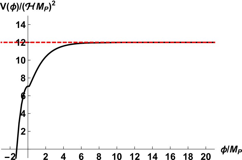
(a)

(b)

Figure 2: (a) Graph of $V(\phi)/(\mathcal{H}M_{\mbox{{\tiny P}}})^{2}$ as a function of $\phi/M_{\mbox{{\tiny P}}}$, for $\Omega=1.5$ (obtained by parametric plotting of the curve $\tau\!\mapsto\!(\phi(\tau)/M_{\mbox{{\tiny P}}},W(\tau)/(\mathcal{H}M_{\mbox{{\tiny P}}})^{2})$; (b) Zoom of (a), showing that $V(\phi)$ has a local minimum and a local maximum near $\phi=0$ for $\Omega=1.5$.

Secondly, let us return to Equations (82) and (84) and note that

$${\phi(\tau)\over M_{\mbox{{\tiny P}}}}=\sqrt{2}\,\log(\mathcal{H}\tau)+O(1)\,,\quad{W(\tau)\over(\mathcal{H}M_{\mbox{{\tiny P}}})^{2}}=12+O\!\left({1\over\mathcal{H}\tau}\right)\quad\;\mbox{for $\tau\to+\infty$}\,;$$ (89)

along with Equation (85), this implies

$${V(\phi)\over(\mathcal{H}M_{\mbox{{\tiny P}}})^{2}}=12+O\big{(}e^{-{\phi/(\sqrt{2}M_{\mbox{{\tiny P}}})}}\big{)}\qquad\mbox{for $\phi\to+\infty$}\,.$$ (90)

Due to Equations (9), (12), (15) and (53), the above relations imply

$$\rho(\tau)\to 0\,,\quad p(\tau)\to 0\,,\quad\rho_{\phi}(\tau)\to 12\,(\mathcal{H}M_{\mbox{{\tiny P}}})^{2}\,,\quad p_{\phi}(\tau)\to-\,12\,(\mathcal{H}M_{\mbox{{\tiny P}}})^{2}\quad\;\mbox{for $\tau\!\to\!+\infty$}\,.$$ (91)

In conclusion, let us point out that Equations (16)–(18) and (76) yield an explicit expression for the coefficient $w_{\phi}(\tau)$ in the field equation of state; this in turns implies the asymptotics

$$w_{\phi}(\tau)=\left\{\!\!\begin{array}[]{ll}\displaystyle{{1\over 3}+O\big{(}(\mathcal{H}\tau)^{2}\big{)}}&\displaystyle{\mbox{for $\tau\to 0$}\,,\vspace{0.1cm}}\\ \displaystyle{-1-{1\over 6\,(\mathcal{H}\tau)^{2}}+O\!\left(\!{1\over(\mathcal{H}\tau)^{3}}\!\right)}&\displaystyle{\mbox{for $\tau\to+\infty$}\,,}\end{array}\right.$$ (92)

which can be commented similarly to Equation (75) of the previous section.

M.G. contributed mainly to aspects of the paper related to the general setting of scalar cosmologies; and D.F. and L.P. contributed mainly to the part of the paper related to Proposition 4 and to the three cosmological models with a phantom field.

This research was funded by: INdAM, Gruppo Nazionale per la Fisica Matematica; Istituto Nazionale di Fisica Nucleare; MIUR, PRIN 2010 Research Project “Geometric and analytic theory of Hamiltonian systems in finite and infinite dimensions”; Università degli Studi di Milano.