Central exclusive diffractive production of $K^{+}K^{-}K^{+}K^{-}$
via the intermediate $\phi\phi$ state in proton-proton collisions

Abstract

We present a study of the exclusive $pp\to ppK^{+}K^{-}K^{+}K^{-}$ reaction at high energies. We consider diffractive mechanisms with the intermediate $\phi\phi$ state with its decay into the $K^{+}K^{-}K^{+}K^{-}$ system. We include the $\phi(1020)$ $\hat{t}/\hat{u}$-channel exchanges and the $f_{2}(2340)$ $s$-channel exchange mechanism. This $f_{2}$ state is a candidate for a tensor glueball. We discuss the possibility to use the $pp\to pp\phi\phi$ process in identifying the odderon exchange. An upper limit for the $\mathbb{P}\mathbb{O}\phi$ coupling is extracted from the WA102 experimental data. The amplitudes for the processes are formulated within the tensor-pomeron and vector-odderon approach. We adjust parameters of our model to the WA102 data and present several predictions for the ALICE, ATLAS, CMS and LHCb experiments. Integrated cross sections of order of a few nb are obtained including the experimental cuts relevant for the LHC experiments. The distributions in the four-kaon invariant mass, rapidity distance between the two $\phi$ mesons, special “glueball filter variable”, proton-proton relative azimuthal angle are presented. The distribution in rapidity difference of both $\phi$-mesons could shed light on the $f_{2}(2340)\to\phi\phi$ coupling, not known at present. We discuss the possible role of the $f_{0}(2100)$, $\eta(2225)$, and $X(2500)$ resonances observed in the $\phi\phi$ channel in radiative decays of $J/\psi$. Using typical kinematic cuts for LHC experiments we find from our model that the odderon-exchange contribution should be distinguishable from other contributions for large rapidity distance between the $\phi$ mesons and in the region of large four-kaon invariant masses. At least, it should be possible to derive an upper limit on the odderon contribution in this reaction.

I Introduction

Diffractive studies are one of the important parts of the physics program for the RHIC and LHC experiments. A particularly interesting class is the central-exclusive-production (CEP) processes, where all centrally produced particles are detected; see Sec. 5 of N.Cartiglia:2015gve . In recent years, there has been a renewed interest in exclusive production of $\pi^{+}\pi^{-}$ pairs at high energies related to successful experiments by the CDF Aaltonen:2015uva and the CMS Khachatryan:2017xsi collaborations. These measurements are important in the context of resonance production, in particular, in searches for glueballs. The experimental data on central exclusive $\pi^{+}\pi^{-}$ production measured at Fermilab and CERN all show visible structures in the $\pi^{+}\pi^{-}$ invariant mass. As we discussed in Ref. Lebiedowicz:2016ioh the pattern of these structures has a mainly resonant origin and is very sensitive to the cuts used in a particular experiment (usually these cuts are different for different experiments). In the CDF and CMS experiments, the large rapidity gaps around the centrally produced dimeson system are checked, but the forward- and backward-going (anti)protons are not detected. Preliminary results of similar CEP studies have been presented by the ALICE Schicker:2012nn and LHCb McNulty:2016sor collaborations at the LHC. Although such results will have a diffractive nature, further efforts are needed to ensure their exclusivity. Ongoing and planned experiments at the RHIC (see, e.g., Sikora:2018cyk ) and future experiments at the LHC will be able to detect all particles produced in central exclusive processes, including the forward- and backward-going protons. Feasibility studies for the $pp\to pp\pi^{+}\pi^{-}$ process with tagging of the scattered protons as carried out for the ATLAS and ALFA detectors are shown in Staszewski:2011bg . Similar possibilities exist using the CMS and TOTEM detectors; see, e.g., Albrow:2014lrm .

It was known for a long time that the frequently used vector-pomeron model has problems from the point of view of field theory. Taken literally it gives opposite signs for $pp$ and $\bar{p}p$ total cross sections. A way to solve these problems was discussed in Nachtmann:1991ua , where the pomeron was described as a coherent superposition of exchanges with spin 2 + 4 + 6 + … The same idea is realised in the tensor-pomeron model formulated in Ewerz:2013kda . In this model, pomeron exchange can effectively be treated as the exchange of a rank-2 symmetric tensor. In Ewerz:2016onn it was shown that the tensor-pomeron model is consistent with the experimental data on the helicity structure of proton-proton elastic scattering at $\sqrt{s}=200$ GeV and small $|t|$ from the STAR experiment Adamczyk:2012kn . In Ref. Lebiedowicz:2013ika the tensor-pomeron model was applied to the diffractive production of several scalar and pseudoscalar mesons in the reaction $pp\to ppM$. In Bolz:2014mya an extensive study of the photoproduction reaction $\gamma p\to\pi^{+}\pi^{-}p$ in the framework of the tensor-pomeron model was presented. The resonant ($\rho^{0}\to\pi^{+}\pi^{-}$) and nonresonant (Drell-Söding) photon-pomeron/reggeon $\pi^{+}\pi^{-}$ production in $pp$ collisions was studied in Lebiedowicz:2014bea . The central exclusive diffractive production of the $\pi^{+}\pi^{-}$ continuum together with the dominant scalar $f_{0}(500)$, $f_{0}(980)$, and tensor $f_{2}(1270)$ resonances was studied by us in Lebiedowicz:2016ioh . The $\rho^{0}$ meson production associated with a very forward/backward $\pi N$ system in the $pp\to pp\rho^{0}\pi^{0}$ and $pp\to pn\rho^{0}\pi^{+}$ processes was discussed in Lebiedowicz:2016ryp . Also the central exclusive $\pi^{+}\pi^{-}\pi^{+}\pi^{-}$ production via the intermediate $\sigma\sigma$ and $\rho^{0}\rho^{0}$ states in $pp$ collisions was considered in Lebiedowicz:2016zka . In Lebiedowicz:2018sdt the $pp\to ppp\bar{p}$ reaction was studied. Recently, in Lebiedowicz:2018eui , the exclusive diffractive production of the $K^{+}K^{-}$ in the continuum and via the dominant scalar $f_{0}(980)$, $f_{0}(1500)$, $f_{0}(1710)$, and tensor $f_{2}(1270)$, $f^{\prime}_{2}(1525)$ resonances, as well as the $K^{+}K^{-}$ photoproduction contributions, was discussed in detail. In Lebiedowicz:2019por a possibility to extract the pomeron-pomeron-$f_{2}(1270)$ [$\mathbb{P}\mathbb{P}f_{2}(1270)$] couplings from the analysis of angular distributions in the $\pi^{+}\pi^{-}$ rest system was studied.

The identification of glueballs in the $pp\to pp\pi^{+}\pi^{-}$ reaction, being analysed by the STAR, ALICE, ATLAS, CMS, and LHCb collaborations, can be rather difficult, as the di-pion spectrum is dominated by the $q\bar{q}$ states and mixing of the pure glueball states with nearby $q\bar{q}$ mesons is possible. The partial wave analyses of future experimental data could be used in this context. Studies of different decay channels in central exclusive production would be very valuable. One of the promising reactions is $pp\to pp\phi\phi$ with both $\phi\equiv\phi(1020)$ mesons decaying into the $K^{+}K^{-}$ channel. The advantage of this process for experimental studies is the following. The $\phi(1020)$ is a narrow resonance and it can be easily identified in the $K^{+}K^{-}$ spectra. On the other hand, non-$\phi\phi$ backgrounds in these spectra should have a broad distribution. However, identification of possible glueball-like states in this channel requires calculation/estimation both of resonant and continuum processes. It is known from the WA102 analysis of various channels that the so-called “glueball-filter variable” ($\rm{dP_{t}}$) Close:1997pj , defined by the difference of the transverse momentum vectors of the outgoing protons, can be used to select out known $q\bar{q}$ states from non-$q\bar{q}$ candidates. It was observed by the WA102 Collaboration (see, e.g., Barberis:1996iq ; Barberis:1997ve ; Barberis:1998ax ; Barberis:1999cq ; Barberis:2000em , Kirk:2000ws ; Kirk:2014nwa ) that all the undisputed $q\bar{q}$ states are suppressed at small $\rm{dP_{t}}$ in contrast to glueball candidates. It is therefore interesting to make a similar study of the $\rm{dP_{t}}$ dependence for the $\phi\phi$ system decaying into $K^{+}K^{-}K^{+}K^{-}$ in central $pp$ collisions at the LHC.

Structures in the $\phi\phi$ invariant-mass spectrum were observed by several experiments. Broad $J^{PC}=2^{++}$ structures around 2.3 GeV were reported in the inclusive $\pi^{-}Be\to\phi\phi+X$ reaction Booth:1985kv ; Booth:1985kr , in the exclusive $\pi^{-}p\to\phi\phi n$ Etkin:1985se ; Etkin:1987rj and $K^{-}p\to\phi\phi\Lambda$ Aston:1989gx ; Aston:1990wf reactions, in central production Armstrong:1986ky ; Armstrong:1989hz ; Barberis:1998bq , and in $p\bar{p}$ annihilations Evangelista:1998zg . In the radiative decay $J/\psi\to\gamma\phi\phi$ an enhancement near ${\rm M}_{\phi\phi}=2.25$ GeV with preferred $J^{PC}=0^{-+}$ was observed Bisello:1986pt ; Bai:1990hk ; Ablikim:2008ac ; Ablikim:2016hlu . The last partial wave analysis Ablikim:2016hlu shows that the $\eta(2225)$ state is significant, but a large contribution from the direct decay of $J/\psi\to\gamma\phi\phi$, modeled by a $0^{-+}$ phase space distribution of the $\phi\phi$ system, was also found there. Also the scalar state $f_{0}(2100)$ and two additional pseudoscalar states, $\eta(2100)$ and the $X(2500)$, were observed. Three tensor states, $f_{2}(2010)$, $f_{2}(2300)$, and $f_{2}(2340)$, observed previously in Etkin:1985se ; Etkin:1987rj , were also observed in $J/\psi\to\gamma\phi\phi$. It was concluded there that the tensor spectrum is dominated by the $f_{2}(2340)$. The nature of these resonances is not understood at present and a tensor glueball has still not been clearly identified. According to lattice-QCD simulations, the lightest tensor glueball has a mass between 2.2 and 2.4 GeV; see, e.g., Morningstar:1997ff ; Morningstar:1999rf ; Hart:2001fp ; Loan:2005ff ; Gregory:2012hu ; Chen:2005mg ; Sun:2017ipk . The $f_{2}(2300)$ and $f_{2}(2340)$ states are good candidates to be tensor glueballs. For an experimental work indicating a possible tensor glueball, see Longacre:2004jn . Also lattice-QCD predictions for the production rate of the pure gauge tensor glueball in radiative $J/\psi$ decays Yang:2013xba are consistent with the large production rate of the $f_{2}(2340)$ in the $\eta\eta$ Ablikim:2013hq , $\phi\phi$ Ablikim:2016hlu and $K_{S}K_{S}$ Ablikim:2018izx channels.

We have presented here some discussion of the role of resonances with masses around 2 GeV in connection with their possible glueball interpretations. With this we want to underline the importance of the study of resonances in this mass range. Our present paper aims to facilitate such studies, for instance, by investigating in detail the interplay of continuum and resonance production of $\phi\phi$ states. But we emphasize that in the following we make no assumptions if the resonances considered are glueballs or not.

In the present paper we wish to concentrate on the CEP of four charged kaons via the intermediate $\phi\phi$ state. Here we shall give explicit expressions for the $pp\to pp\phi\phi$ amplitudes involving the pomeron-pomeron fusion to $\phi\phi$ ($\mathbb{P}\mathbb{P}\to\phi\phi$) through the continuum processes, due to the $\hat{t}$- and $\hat{u}$-channel reggeized $\phi$-meson, photon, and odderon exchanges, as well as through the $s$-channel resonance reaction ($\mathbb{P}\mathbb{P}\to f_{2}(2340)\to\phi\phi$). The pseudoscalar mesons having $I^{G}=0^{+}$ and $J^{PC}=0^{-+}$ can also be produced in pomeron-pomeron fusion and may contribute to our reaction if they decay to $\phi\phi$. Possible candidates are, e.g., $\eta(2225)$ and $X(2500)$, which were observed in radiative decays of $J/\psi$ Ablikim:2016hlu . The same holds for scalar states with $I^{G}=0^{+}$ and $J^{PC}=0^{++}$, for example, the scalar $f_{0}(2100)$ meson. We will comment on the possible influence of these contributions for the CEP of $\phi\phi$ pairs. Some model parameters will be determined from the comparison to the WA102 experimental data Barberis:1998bq ; Barberis:2000em . In order to give realistic predictions we shall include absorption effects calculated at the amplitude level and related to the $pp$ nonperturbative interactions.

II Exclusive diffractive production of four kaons

In the present paper we consider the $2\to 6$ process, CEP of four $K$ mesons, with the intermediate $\phi(1020)\phi(1020)$ resonance pair,

$$pp\to pp\,\phi\phi\to ppK^{+}K^{-}K^{+}K^{-}\,.$$ (1)

In Fig. 1 we show diagrams for this process which are expected to be the most important ones at high energies since they involve pomeron exchanges. Figure 1 (a) shows the continuum process. In Fig. 1 (b) we have the process with intermediate production of an $f_{2}$ resonance,

$$pp\to pp\,(\mathbb{P}\mathbb{P}\to f_{2}\to\phi\phi)\to pp\,K^{+}K^{-}K^{+}K^{-}\,.$$ (2)

In the place of the $f_{2}$ we can also have an $f_{0}$- and an $\eta$-type resonance. That is, we treat effectively the $2\to 6$ processes (1) and (2) as arising from the $2\to 4$ process, the central diffractive production of two vector $\phi(1020)$ mesons in proton-proton collisions.

In Fig. 1 (a) we have the exchange of a $\phi$ or $\phi_{\mathbb{R}}$ reggeon, depending on the kinematics, as we shall discuss in detail below. In place of the $\phi$ or $\phi_{\mathbb{R}}$ we can, in principle, also have an $\omega$ or $\omega_{\mathbb{R}}$. But these contributions are expected to be very small since the $\phi$ is nearly a pure $s\bar{s}$ state, the $\omega$ nearly a pure $u\bar{u}+d\bar{d}$ state. In the following we shall, therefore, neglect such contributions.

The production of $\phi\phi$ can also occur through diagrams of the type of Fig. 1 but with reggeons in the place of the pomerons. For example, in Fig. 1 (a) we can replace the pomerons by $\phi_{\mathbb{R}}$ reggeons and the intermediate $\phi$ by a pomeron. In Fig. 1 (b) we can replace one or two pomerons by one or two $f_{2\mathbb{R}}$ reggeons. For high energies and central $\phi\phi$ production such reggeon contributions are expected to be small and we shall not consider them in our present paper. We shall treat in detail the diagrams with pomeron exchange (Fig. 1) and diagrams involving odderon and also photon exchange; see Figs. 2 and 4 below.

A resonance produced in pomeron-pomeron fusion must have $I^{G}=0^{+}$ and charge conjugation $C=+1$, but it may have various spin and parity quantum numbers. See e.g. the discussion in Appendix A of Lebiedowicz:2013ika .

In Table 1 we have listed intermediate resonances that can contribute to the $pp\to pp\phi\phi$ reaction (2) and to other processes with two vector mesons in the final state. It must be noted that the scalar state $f_{0}(2100)$ and three pseudoscalar states, $\eta(2100)$, $\eta(2225)$, and $X(2500)$, which were observed in the process $J/\psi\to\gamma\phi\phi$ Ablikim:2016hlu , are only listed in PDG Tanabashi:2018oca and are not included in the summary tables. Clearly these states need confirmation.

Table 1: A list of resonances, up to a mass of 2500 MeV, that decay into a vector meson pair. The meson masses $m$ and their total widths $\Gamma$ are taken from PDG Tanabashi:2018oca . For $\eta(2100)$ and $X(2500)$, the information is taken from Ablikim:2016hlu . In the first column, the $\bullet$ symbol indicates rather established particles. In the fifth column, the (?) symbol denotes the states that need further experimental confirmation.

Meson	$I^{G}J^{PC}$	$m$ (MeV)	$\Gamma$ (MeV)	$\phi\phi$	$K^{*0}\bar{K}^{*0}$	$\rho^{0}\rho^{0}$	$\omega\omega$
$\bullet\,f_{1}(1285)$	$0^{+}1^{++}$	$1281.9\pm 0.5$	$22.7\pm 1.1$			Seen
$\bullet\,f_{0}(1370)$	$0^{+}0^{++}$	$1200-1500$	$200-500$			Dominant	Not seen
$\bullet\,f_{0}(1500)$	$0^{+}0^{++}$	$1504\pm 6$	$109\pm 7$			Seen
$f_{2}(1565)$	$0^{+}2^{++}$	$1562\pm 13$	$134\pm 8$			Seen	Seen
$f_{2}(1640)$	$0^{+}2^{++}$	$1639\pm 6$	$99^{+60}_{-40}$				Seen
$\bullet\,f_{0}(1710)$	$0^{+}0^{++}$	$1723^{+6}_{-5}$	$139\pm 8$				Seen
$\eta(1760)$	$0^{+}0^{-+}$	$1751\pm 15$	$240\pm 30$			Seen	Seen
$f_{2}(1910)$	$0^{+}2^{++}$	$1903\pm 9$	$196\pm 31$			Seen	Seen
$\bullet\,f_{2}(1950)$	$0^{+}2^{++}$	$1944\pm 12$	$472\pm 18$		Seen
$\bullet\,f_{2}(2010)$	$0^{+}2^{++}$	$2011^{+60}_{-80}$	$202\pm 60$	Seen
$f_{0}(2020)$	$0^{+}0^{++}$	$1992\pm 16$	$442\pm 60$			Seen	Seen
$f_{0}(2100)$	$0^{+}0^{++}$	$2101\pm 7$	$224^{+23}_{-21}$	Seen (?)
$\eta(2100)$	$0^{+}0^{-+}$	$2050^{+30+75}_{-24-26}$ Ablikim:2016hlu	$250^{+36+181}_{-30-164}$ Ablikim:2016hlu	Seen (?)
$\bullet\,f_{4}(2050)$	$0^{+}4^{++}$	$2018\pm 11$	$237\pm 18$				Seen
$f_{J}(2220)$	$0^{+}(2^{++}\,\rm{or}\,4^{++})$	$2231.1\pm 3.5$	$23^{+8}_{-7}$	Not seen
$\eta(2225)$	$0^{+}0^{-+}$	$2221^{+13}_{-10}$	$185^{+40}_{-20}$	Seen (?)
$\bullet\,f_{2}(2300)$	$0^{+}2^{++}$	$2297\pm 28$	$149\pm 40$	Seen
$f_{4}(2300)$	$0^{+}4^{++}$	$2320\pm 60$	$250\pm 80$			Seen	Seen
$\bullet\,f_{2}(2340)$	$0^{+}2^{++}$	$2345^{+50}_{-40}$	$322^{+70}_{-60}$	Seen
$X(2500)$	$0^{+}0^{-+}$	$2470^{+15+101}_{-19-23}$ Ablikim:2016hlu	$230^{+64+56}_{-35-33}$ Ablikim:2016hlu	Seen (?)

To calculate the total cross section for the $2\to 4$ reactions one has to calculate the 8-dimensional phase-space integral numerically Lebiedowicz:2009pj . Some modifications of the $2\to 4$ reaction are needed to simulate the $2\to 6$ reaction with $K^{+}K^{-}K^{+}K^{-}$ in the final state. For example, since the $\phi(1020)$ is an unstable particle one has to include a smearing of the $\phi$ masses due to their resonance distribution. Then, the general cross-section formula can be written approximately as

$${\sigma}_{2\to 6} = [{\cal B}(\phi(1020)\to K^{+}K^{-})]^{2}$$ (3)

$$\times\int_{2m_{K}}^{{\rm max}\{m_{X_{3}}\}}\int_{2m_{K}}^{{\rm max}\{m_{X_{4}}\}}{\sigma}_{2\to 4}(...,m_{X_{3}},m_{X_{4}})\,f_{\phi}(m_{X_{3}})\,f_{\phi}(m_{X_{4}})\,dm_{X_{3}}\,dm_{X_{4}}\qquad$$

with the branching fraction ${\cal B}(\phi(1020)\to K^{+}K^{-})=0.492$ Tanabashi:2018oca . We use for the calculation of the decay process $\phi(1020)\to K^{+}K^{-}$ the spectral function

$$f_{\phi}(m_{X_{i}})=C_{\phi}\,\left(1-\dfrac{4m_{K}^{2}}{m_{X_{i}}^{2}}\right)^{3/2}\frac{\frac{2}{\pi}{m_{\phi}^{2}}\Gamma_{\phi}}{(m_{X_{i}}^{2}-m_{\phi}^{2})^{2}+m_{\phi}^{2}\Gamma_{\phi}^{2}}\,,$$ (4)

where $i=3,4$, $\Gamma_{\phi}$ is the total width of the $\phi(1020)$ resonance, $m_{\phi}$ its mass, and $C_{\phi}=64.1$ is found from the condition

$$\int_{2m_{K}}^{\infty}f_{\phi}(m_{X_{i}})dm_{X_{i}}=1\,.$$ (5)

The quantity $\left(1-4m_{K}^{2}/m_{X_{i}}^{2}\right)^{3/2}$ smoothly decreases the spectral function when approaching the $K^{+}K^{-}$ threshold, $m_{X_{i}}\to 2m_{K}$, and takes into account the angular momentum $l=1$ of the $K^{+}K^{-}$ state.

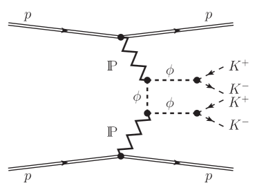
(a) (b)

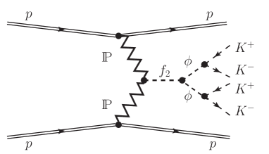
Figure 1: The “Born-level” diagrams for double pomeron central exclusive $\phi\phi$ production and their subsequent decays into $K^{+}K^{-}K^{+}K^{-}$ in proton-proton collisions: (a) continuum $\phi\phi$ production; (b) $\phi\phi$ production via an $f_{2}$ resonance. Other resonances, e.g. of $f_{0}$- and $\eta$-type, can also contribute here.

To include experimental cuts on charged kaons we perform the decays of $\phi$ mesons isotropically in the $\phi$ rest frames and then use relativistic transformations to the overall center-of-mass frame.

In principle, there are other processes contributing to the $K^{+}K^{-}K^{+}K^{-}$ final state, for example, direct $K^{+}K^{-}K^{+}K^{-}$ continuum production and processes with $f_{0,2}$ resonances:

$$pp\to pp\,K^{+}K^{-}K^{+}K^{-}\,,$$ (6)

$$pp\to pp\,f_{0,2}\,K^{+}K^{-}\to pp\,K^{+}K^{-}K^{+}K^{-}\,,$$ (7)

$$pp\to pp\,f_{0,2}\,f_{0,2}\to pp\,K^{+}K^{-}K^{+}K^{-}\,,$$ (8)

$$pp\to pp\,(f_{2}\to f_{0}\,f_{0})\to pp\,K^{+}K^{-}K^{+}K^{-}\,.$$ (9)

Here $f_{0,2}$ stands for one of the scalar or tensor mesons decaying to $K^{+}K^{-}$. It should be noted that a complete theoretical model of the $pp\to ppK^{+}K^{-}K^{+}K^{-}$ process should include interference effects of the processes (1), (2), and (6)–(9). However, such a detailed study of the $pp\to ppK^{+}K^{-}K^{+}K^{-}$ reaction will only be necessary once high-energy experimental data for the purely exclusive measurements will be available. We leave this interesting problem for future studies. The GenEx Monte Carlo generator Kycia:2014hea ; Kycia:2017ota could be used in this context. We refer the reader to Ref. Kycia:2017iij where a first calculation of four-pion continuum production in the $pp\to pp\pi^{+}\pi^{-}\pi^{+}\pi^{-}$ reaction with the help of the GenEx code was performed.

III The reaction $pp\to pp\phi\phi$

Here we discuss the exclusive production of $\phi\phi\equiv\phi(1020)\phi(1020)$ in proton-proton collisions,

$$p(p_{a},\lambda_{a})+p(p_{b},\lambda_{b})\to p(p_{1},\lambda_{1})+\phi(p_{3},\lambda_{3})+\phi(p_{4},\lambda_{4})+p(p_{2},\lambda_{2})\,,$$ (10)

where $p_{a,b}$, $p_{1,2}$ and $\lambda_{a,b},\lambda_{1,2}=\pm\frac{1}{2}$ denote the four-momenta and helicities of the protons and $p_{3,4}$ and $\lambda_{3,4}=0,\pm 1$ denote the four-momenta and helicities of the $\phi$ mesons, respectively.

The amplitude for the reaction (10) can be written as

$$\begin{split}{\cal M}_{\lambda_{a}\lambda_{b}\to\lambda_{1}\lambda_{2}\phi\phi}=\left(\epsilon^{(\phi)}_{\rho_{3}}(\lambda_{3})\right)^{*}\left(\epsilon^{(\phi)}_{\rho_{4}}(\lambda_{4})\right)^{*}{\cal M}^{\rho_{3}\rho_{4}}_{\lambda_{a}\lambda_{b}\to\lambda_{1}\lambda_{2}\phi\phi}\,,\end{split}$$ (11)

where $\epsilon^{(\phi)}_{\mu}(\lambda)$ are the polarisation vectors of the $\phi$ meson.

We consider here unpolarised protons in the initial state and no observation of polarisations in the final state. Therefore, we have to insert in (3) the cross section $\sigma_{2\to 4}$ summed over the $\phi$ meson polarisations. The spin sum for a $\phi$ meson of momentum $k$ and squared mass $k^{2}=m_{X}^{2}$ is

$$\begin{split}\sum_{\lambda=0,\pm 1}\epsilon^{(\phi)\,\mu}(\lambda)\left(\epsilon^{(\phi)\,\nu}(\lambda)\right)^{*}=-g^{\mu\nu}+\dfrac{k^{\mu}k^{\nu}}{m_{X}^{2}}\,.\end{split}$$ (12)

But in our model the $k^{\mu}k^{\nu}$ terms do not contribute to the cross section since we have the relations

$$\begin{split}p_{3\,\rho_{3}}{\cal M}^{\rho_{3}\rho_{4}}_{\lambda_{a}\lambda_{b}\to\lambda_{1}\lambda_{2}\phi\phi}=0\,,\qquad p_{4\,\rho_{4}}{\cal M}^{\rho_{3}\rho_{4}}_{\lambda_{a}\lambda_{b}\to\lambda_{1}\lambda_{2}\phi\phi}=0\,,\end{split}$$ (13)

which will be shown below in Secs. III.1 and III.2.

Taking also into account the statistical factor $\frac{1}{2}$ due to the identity of the two $\phi$ mesons we get for the amplitudes squared [to be inserted in $\sigma_{2\to 4}$ in (3)]

$$\begin{split}\frac{1}{2}\frac{1}{4}\sum_{\rm{spins}}\Big{|}{\cal M}_{\lambda_{a}\lambda_{b}\to\lambda_{1}\lambda_{2}\phi\phi}\Big{|}^{2}=\frac{1}{8}\sum_{\lambda_{a},\lambda_{b},\lambda_{1},\lambda_{2}}\left({\cal M}^{\sigma_{3}\sigma_{4}}_{\lambda_{a}\lambda_{b}\to\lambda_{1}\lambda_{2}\phi\phi}\right)^{*}{\cal M}^{\rho_{3}\rho_{4}}_{\lambda_{a}\lambda_{b}\to\lambda_{1}\lambda_{2}\phi\phi}\,g_{\sigma_{3}\rho_{3}}\,g_{\sigma_{4}\rho_{4}}\,.\end{split}$$ (14)

To give the full physical amplitude for the $pp\to pp\phi\phi$ reaction we include absorptive corrections to the Born amplitudes discussed below. For the details of how to include the $pp$-rescattering corrections in the eikonal approximation for the four-body reaction see Sec. 3.3 of Lebiedowicz:2014bea .

III.1 $\phi$-meson exchange mechanism

The diagram for the $\phi\phi$ production with an intermediate $\phi$-meson exchange is shown in Fig. 1 (a). The Born-level amplitude can be written as the sum

$${\cal M}^{(\phi{\rm-exchange})\,\rho_{3}\rho_{4}}_{\lambda_{a}\lambda_{b}\to\lambda_{1}\lambda_{2}\phi\phi}={\cal M}^{({\hat{t}})\,\rho_{3}\rho_{4}}_{\lambda_{a}\lambda_{b}\to\lambda_{1}\lambda_{2}\phi\phi}+{\cal M}^{({\hat{u}})\,\rho_{3}\rho_{4}}_{\lambda_{a}\lambda_{b}\to\lambda_{1}\lambda_{2}\phi\phi}$$ (15)

with the $\hat{t}$- and $\hat{u}$-channel amplitudes:

$$\begin{split}{\cal M}^{({\hat{t}})}_{\rho_{3}\rho_{4}}=&(-i)\bar{u}(p_{1},\lambda_{1})i\Gamma^{(\mathbb{P}pp)}_{\mu_{1}\nu_{1}}(p_{1},p_{a})u(p_{a},\lambda_{a})\,i\Delta^{(\mathbb{P})\,\mu_{1}\nu_{1},\alpha_{1}\beta_{1}}(s_{13},t_{1})\\ &\times i\Gamma^{(\mathbb{P}\phi\phi)}_{\rho_{1}\rho_{3}\alpha_{1}\beta_{1}}(\hat{p}_{t},-p_{3})\,i\Delta^{(\phi)\,\rho_{1}\rho_{2}}(\hat{p}_{t})\,i\Gamma^{(\mathbb{P}\phi\phi)}_{\rho_{4}\rho_{2}\alpha_{2}\beta_{2}}(p_{4},\hat{p}_{t})\\ &\times i\Delta^{(\mathbb{P})\,\alpha_{2}\beta_{2},\mu_{2}\nu_{2}}(s_{24},t_{2})\,\bar{u}(p_{2},\lambda_{2})i\Gamma^{(\mathbb{P}pp)}_{\mu_{2}\nu_{2}}(p_{2},p_{b})u(p_{b},\lambda_{b})\,,\end{split}$$ (16)

$$\begin{split}{\cal M}^{({\hat{u}})}_{\rho_{3}\rho_{4}}=&(-i)\bar{u}(p_{1},\lambda_{1})i\Gamma^{(\mathbb{P}pp)}_{\mu_{1}\nu_{1}}(p_{1},p_{a})u(p_{a},\lambda_{a})\,i\Delta^{(\mathbb{P})\,\mu_{1}\nu_{1},\alpha_{1}\beta_{1}}(s_{14},t_{1})\\ &\times i\Gamma^{(\mathbb{P}\phi\phi)}_{\rho_{4}\rho_{1}\alpha_{1}\beta_{1}}(p_{4},\hat{p}_{u})\,i\Delta^{(\phi)\,\rho_{1}\rho_{2}}(\hat{p}_{u})\,i\Gamma^{(\mathbb{P}\phi\phi)}_{\rho_{2}\rho_{3}\alpha_{2}\beta_{2}}(\hat{p}_{u},-p_{3})\\ &\times i\Delta^{(\mathbb{P})\,\alpha_{2}\beta_{2},\mu_{2}\nu_{2}}(s_{23},t_{2})\,\bar{u}(p_{2},\lambda_{2})i\Gamma^{(\mathbb{P}pp)}_{\mu_{2}\nu_{2}}(p_{2},p_{b})u(p_{b},\lambda_{b})\,,\end{split}$$ (17)

where $\hat{p}_{t}=p_{a}-p_{1}-p_{3}$, $\hat{p}_{u}=p_{4}-p_{a}+p_{1}$, $s_{ij}=(p_{i}+p_{j})^{2}$, $t_{1}=(p_{1}-p_{a})^{2}$, and $t_{2}=(p_{2}-p_{b})^{2}$. Here $\Delta^{(\mathbb{P})}$ and $\Gamma^{(\mathbb{P}pp)}$ denote the effective propagator and proton vertex function, respectively, for the tensorial pomeron. The corresponding expressions, as given in Sec. 3 of Ewerz:2013kda , are as follows:

$$i\Delta^{(\mathbb{P})}_{\mu\nu,\kappa\lambda}(s,t) = \frac{1}{4s}\left(g_{\mu\kappa}g_{\nu\lambda}+g_{\mu\lambda}g_{\nu\kappa}-\frac{1}{2}g_{\mu\nu}g_{\kappa\lambda}\right)(-is\alpha^{\prime}_{\mathbb{P}})^{\alpha_{\mathbb{P}}(t)-1}\,,$$ (18)

$$i\Gamma_{\mu\nu}^{(\mathbb{P}pp)}(p^{\prime},p) = -i3\beta_{\mathbb{P}NN}F_{1}(t)\left\{\frac{1}{2}\left[\gamma_{\mu}(p^{\prime}+p)_{\nu}+\gamma_{\nu}(p^{\prime}+p)_{\mu}\right]-\frac{1}{4}g_{\mu\nu}(p\!\!\!/^{\prime}+p\!\!\!/)\right\},\qquad\quad$$ (19)

where $\beta_{\mathbb{P}NN}=1.87$ GeV^-1. For extensive discussions of the properties of these terms we refer to Ewerz:2013kda . Here the pomeron trajectory $\alpha_{\mathbb{P}}(t)$ is assumed to be of standard linear form (see, e.g., Donnachie:1992ny ; Donnachie:2002en ):

$$\alpha_{\mathbb{P}}(t)=\alpha_{\mathbb{P}}(0)+\alpha^{\prime}_{\mathbb{P}}\,t,$$

$$\alpha_{\mathbb{P}}(0)=1.0808\,,\;\;\alpha^{\prime}_{\mathbb{P}}=0.25\;{\rm GeV}^{-2}\,.$$ (20)

Our ansatz for the $\mathbb{P}\phi\phi$ vertex follows the one for the $\mathbb{P}\rho\rho$ in (3.47) of Ewerz:2013kda with the replacements $a_{\mathbb{P}\rho\rho}\to a_{\mathbb{P}\phi\phi}$ and $b_{\mathbb{P}\rho\rho}\to b_{\mathbb{P}\phi\phi}$. This was already used in Sec. IV B of Lebiedowicz:2018eui . The $\mathbb{P}\phi\phi$ vertex function is taken with the same Lorentz structure as for $f_{2}\gamma\gamma$ defined in (3.39) of Ewerz:2013kda . With $k^{\prime},\mu$ and $k,\nu$ the momentum and vector index of the outgoing and incoming $\phi$, respectively, and $\kappa\lambda$ the pomeron indices, the $\mathbb{P}\phi\phi$ vertex reads

$$i\Gamma^{(\mathbb{P}\phi\phi)}_{\mu\nu\kappa\lambda}(k^{\prime},k)=iF_{M}((k^{\prime}-k)^{2})\left[2a_{\mathbb{P}\phi\phi}\,\Gamma^{(0)}_{\mu\nu\kappa\lambda}(k^{\prime},-k)\,-b_{\mathbb{P}\phi\phi}\,\Gamma^{(2)}_{\mu\nu\kappa\lambda}(k^{\prime},-k)\right]\,$$ (21)

with two rank-four tensor functions,

$$\Gamma_{\mu\nu\kappa\lambda}^{(0)}(k_{1},k_{2})=\Big{[}(k_{1}\cdot k_{2})g_{\mu\nu}-k_{2\mu}k_{1\nu}\Big{]}\Big{[}k_{1\kappa}k_{2\lambda}+k_{2\kappa}k_{1\lambda}-\frac{1}{2}(k_{1}\cdot k_{2})g_{\kappa\lambda}\Big{]}\,,$$ (22)

$$\Gamma_{\mu\nu\kappa\lambda}^{(2)}(k_{1},k_{2})=\,(k_{1}\cdot k_{2})(g_{\mu\kappa}g_{\nu\lambda}+g_{\mu\lambda}g_{\nu\kappa})+g_{\mu\nu}(k_{1\kappa}k_{2\lambda}+k_{2\kappa}k_{1\lambda})$$

$$\qquad\qquad\qquad\quad-k_{1\nu}k_{2\lambda}g_{\mu\kappa}-k_{1\nu}k_{2\kappa}g_{\mu\lambda}-k_{2\mu}k_{1\lambda}g_{\nu\kappa}-k_{2\mu}k_{1\kappa}g_{\nu\lambda}$$

$$\qquad\qquad\qquad\quad-[(k_{1}\cdot k_{2})g_{\mu\nu}-k_{2\mu}k_{1\nu}]\,g_{\kappa\lambda}\,;$$ (23)

see Eqs. (3.18) and (3.19) of Ewerz:2013kda . In (21) the coupling parameters $a_{\mathbb{P}\phi\phi}$ and $b_{\mathbb{P}\phi\phi}$ have dimensions GeV^-3 and GeV^-1, respectively. In Lebiedowicz:2018eui we have fixed the coupling parameters of the tensor pomeron to the $\phi$ meson based on the HERA experimental data for the $\gamma p\to\phi p$ reaction Derrick:1996af ; Breitweg:1999jy . We take the coupling constants $a_{\mathbb{P}\phi\phi}=0.49$ GeV^-3 and $b_{\mathbb{P}\phi\phi}=4.27$ GeV^-1 from Table II of Lebiedowicz:2018eui (see also Sec. IV B there).

In the hadronic vertices we should take into account form factors since the hadrons are extended objects. The form factors $F_{1}(t)$ in (19) and $F_{M}(t)$ in (21) are chosen here as the electromagnetic form factors only for simplicity,

$$F_{1}(t)=\frac{4m_{p}^{2}-2.79\,t}{(4m_{p}^{2}-t)(1-t/m_{D}^{2})^{2}}\,,$$ (24)

$$F_{M}(t)=\frac{1}{1-t/\Lambda_{0}^{2}}\,;$$ (25)

see Eqs. (3.29) and (3.34) of Ewerz:2013kda , respectively. In (24) $m_{p}$ is the proton mass and $m_{D}^{2}=0.71$ GeV² is the dipole mass squared. As we discussed in Fig. 6 of Lebiedowicz:2018eui we should take in (25) $\Lambda_{0}^{2}=1.0$ GeV² instead of $\Lambda_{0}^{2}=0.5$ GeV² used for the $\mathbb{P}\rho\rho$ vertex in Ewerz:2013kda .

Then, with the expressions for the propagators, vertices, and form factors, from Ewerz:2013kda ${\cal M}^{\rho_{3}\rho_{4}}$ can be written in the high-energy approximation as

$$\begin{split}&{\cal M}^{(\phi{\rm-exchange})\,\rho_{3}\rho_{4}}_{\lambda_{a}\lambda_{b}\to\lambda_{1}\lambda_{2}\phi\phi}=\;2(p_{1}+p_{a})_{\mu_{1}}(p_{1}+p_{a})_{\nu_{1}}\,\delta_{\lambda_{1}\lambda_{a}}\,F_{1}(t_{1})\,F_{M}(t_{1})\\ &\times\bigg{\{}{V}^{\rho_{3}\rho_{1}\mu_{1}\nu_{1}}(s_{13},t_{1},\hat{p}_{t},p_{3})\;\Delta^{(\phi)}_{\rho_{1}\rho_{2}}(\hat{p}_{t})\;{V}^{\rho_{4}\rho_{2}\mu_{2}\nu_{2}}(s_{24},t_{2},-\hat{p}_{t},p_{4})\,\left[\hat{F}_{\phi}(\hat{p}_{t}^{2})\right]^{2}\\ &\quad\;+{V}^{\rho_{4}\rho_{1}\mu_{1}\nu_{1}}(s_{14},t_{1},-\hat{p}_{u},p_{4})\;\Delta^{(\phi)}_{\rho_{1}\rho_{2}}(\hat{p}_{u})\;{V}^{\rho_{3}\rho_{2}\mu_{2}\nu_{2}}(s_{23},t_{2},\hat{p}_{u},p_{3})\,\left[\hat{F}_{\phi}(\hat{p}_{u}^{2})\right]^{2}\bigg{\}}\\ &\times 2(p_{2}+p_{b})_{\mu_{2}}(p_{2}+p_{b})_{\nu_{2}}\,\delta_{\lambda_{2}\lambda_{b}}\,F_{1}(t_{2})\,F_{M}(t_{2})\,,\end{split}$$ (26)

where ${V}_{\mu\nu\kappa\lambda}$ reads as

$$\begin{split}{V}_{\mu\nu\kappa\lambda}(s,t,k_{2},k_{1})=&\frac{1}{4s}\,3\beta_{\mathbb{P}NN}\,(-is\alpha^{\prime}_{\mathbb{P}})^{\alpha_{\mathbb{P}}(t)-1}\bigg{[}2a_{\mathbb{P}\phi\phi}\Gamma_{\mu\nu\kappa\lambda}^{(0)}(k_{1},k_{2})-b_{\mathbb{P}\phi\phi}\Gamma_{\mu\nu\kappa\lambda}^{(2)}(k_{1},k_{2})\bigg{]}\,.\end{split}$$ (27)

The amplitude (26) contains a form factor $\hat{F}_{\phi}(\hat{p}^{2})$ taking into account the off-shell dependencies of the intermediate $\phi$-mesons. The form factor is normalised to unity at the on-shell point $\hat{F}_{\phi}(m_{\phi}^{2})=1$ and parametrised here in the exponential form,

$$\hat{F}_{\phi}(\hat{p}^{2})=\exp\left(\frac{\hat{p}^{2}-m_{\phi}^{2}}{\Lambda^{2}_{off,E}}\right)\,,$$ (28)

where the cutoff parameter $\Lambda_{off,E}$ could be adjusted to experimental data.

The relations (13) are now easily checked from (26) and (27) using the properties of the tensorial functions (22) and (III.1); see (3.21) of Ewerz:2013kda . We can then make in (26) the following replacement for the $\phi$-meson propagator:

$$\Delta^{(\phi)}_{\rho_{1}\rho_{2}}(\hat{p})\to-g_{\rho_{1}\rho_{2}}\,\Delta^{(\phi)}_{T}(\hat{p}^{2})\,,$$ (29)

where we take for $\hat{p}^{2}<0$, where $\Delta^{(\phi)}_{T}(\hat{p}^{2})$ must be real, the simple lowest order expression $(\Delta^{(\phi)}_{T}(\hat{p}^{2}))^{-1}=\hat{p}^{2}-m_{\phi}^{2}$.

We should take into account the fact that the exchanged intermediate object is not a simple spin-1 particle ($\phi$ meson) but may correspond to a Regge exchange, that is, the reggeization of the intermediate $\phi$ meson is necessary (see, e.g., Lebiedowicz:2016zka ). A simple way to include approximately the “reggeization” of the amplitude given in Eq. (26) is by replacing the $\phi$-meson propagator in both the $\hat{t}$- and $\hat{u}$-channel amplitudes by

$$\Delta^{(\phi)}_{\rho_{1}\rho_{2}}(\hat{p})\to\Delta^{(\phi)}_{\rho_{1}\rho_{2}}(\hat{p})\left(\exp(i\phi(s_{34}))\,\frac{s_{34}}{s_{{\rm thr}}}\right)^{\alpha_{\phi}(\hat{p}^{2})-1}\,,$$ (30)

where

$$s_{34}=(p_{3}+p_{4})^{2}={\rm M}_{\phi\phi}^{2}\,,$$

$$s_{\rm thr}=4m_{\phi}^{2}\,.$$ (31)

Here we assume for the $\phi$ Regge trajectory

$$\alpha_{\phi}(\hat{p}^{2})=\alpha_{\phi}(0)+\alpha^{\prime}_{\phi}\,\hat{p}^{2},$$

$$\alpha_{\phi}(0)=0.1\,,\;\;\alpha^{\prime}_{\phi}=0.9\;{\rm GeV}^{-2}\,;$$ (32)

see Eq. (5.3.1) of Collins:1977 . In order to have the correct phase behaviour we introduced in (30) the function $\exp(i\phi(s_{34}))$ with

$$\phi(s_{34})=\frac{\pi}{2}\exp\left(\frac{s_{\rm thr}-s_{34}}{s_{{\rm thr}}}\right)-\frac{\pi}{2}\,.$$ (33)

This procedure of reggeization assures agreement with mesonic physics in the $\phi\phi$ system close to threshold, $s_{34}=4m_{\phi}^{2}$ (no suppression), and it gives the Regge behaviour at large $s_{34}$. However, some care is needed here, as the reggeization is only expected in general to hold in the $|\hat{p}^{2}|/s_{34}\ll 1$ regime. In the reaction considered, both $\langle-\hat{p}_{t}^{2}\rangle$ and $\langle-\hat{p}_{u}^{2}\rangle$ are of order 1 GeV² (before reggeization) with a cutoff for higher $|\hat{p}^{2}|$ provided in (26) by the form factors $\hat{F}_{\phi}(\hat{p}^{2})$ (28). Therefore, the propagator form in (30) and (33) gives correct Regge behaviour for $s_{34}-4m_{\phi}^{2}\gg 1$ GeV² and $|\hat{p}^{2}|$ limited by the form factors, whereas for smaller $s_{34}$ we have mesonic behaviour.

In Ref. Harland-Lang:2013dia it was argued that the reggeization should not be applied when the rapidity distance between two centrally produced mesons, $\rm{Y_{diff}}=\rm{Y}_{3}-\rm{Y}_{4}$, tends to zero (i.e. for $|\hat{p}^{2}|\sim s_{34}$). Indeed, for small $\rm{Y_{diff}}$ the two $\phi$ mesons may have large transverse momenta leading to a large ${\rm M}_{\phi\phi}$. Clearly this kinematic region has nothing to do with the Regge limit. For large $\rm{Y_{diff}}$, on the other hand, the form factors $\hat{F}_{\phi}(\hat{p}^{2})$ in (26) limit the transverse momenta of the $\phi$’s but ${\rm M}_{\phi\phi}$ will be large. That is, there we are in the Regge limit. To take care of these two different regimes we propose to use, as an alternative to (30), a formula for the $\phi$ propagator which interpolates continuously between the regions of low $\rm{Y_{diff}}$, where we use the standard $\phi$ propagator, and of high $\rm{Y_{diff}}$ where we use the reggeized form (30):

$$\Delta^{(\phi)}_{\rho_{1}\rho_{2}}(\hat{p})\to\Delta^{(\phi)}_{\rho_{1}\rho_{2}}(\hat{p})\,F({\rm Y_{diff}})+\Delta^{(\phi)}_{\rho_{1}\rho_{2}}(\hat{p})\,\left[1-F({\rm Y_{diff}})\right]\left(\exp(i\phi(s_{34}))\,\frac{s_{34}}{s_{\rm thr}}\right)^{\alpha_{\phi}(\hat{p}^{2})-1},\qquad$$ (34)

with a simple function

$$F({\rm Y_{diff}})=\exp\left(-{\rm c_{y}}|{\rm Y_{diff}}|\right)\,.$$ (35)

Here ${\rm c_{y}}$ is an unknown parameter which measures how fast one approaches to the Regge regime.

In Sec. IV below we shall compare the two prescriptions of reggeization, (30) and (34); see Figs. 6 and 10. Furthermore, we shall show in Fig. 12 that a large size of the rapidity gap between the two $\phi$ mesons indeed means automatically also large ${\rm M}_{\phi\phi}$ in our model.

III.2 $f_{2}$ resonance production

Now we consider the amplitude for the reaction (10) through the $s$-channel $f_{2}$-meson exchange as shown in Fig. 1 (b). The $f_{2}(2010)$, $f_{2}(2300)$, and $f_{2}(2340)$ mesons could be considered as potential candidates; see Table 1.

The Born amplitude for the $\mathbb{P}\mathbb{P}$ fusion is given by

$$\begin{split}{\cal M}^{(\mathbb{P}\mathbb{P}\to f_{2}\to\phi\phi)\,\rho_{3}\rho_{4}}_{\lambda_{a}\lambda_{b}\to\lambda_{1}\lambda_{2}\phi\phi}=&(-i)\,\bar{u}(p_{1},\lambda_{1})i\Gamma^{(\mathbb{P}pp)\,\mu_{1}\nu_{1}}(p_{1},p_{a})u(p_{a},\lambda_{a})\;i\Delta^{(\mathbb{P})}_{\mu_{1}\nu_{1},\alpha_{1}\beta_{1}}(s_{1},t_{1})\\ &\times i\Gamma^{(\mathbb{P}\mathbb{P}f_{2})\,\alpha_{1}\beta_{1},\alpha_{2}\beta_{2},\rho\sigma}(q_{1},q_{2})\;i\Delta^{(f_{2})}_{\rho\sigma,\alpha\beta}(p_{34})\;i\Gamma^{(f_{2}\phi\phi)\,\alpha\beta\rho_{3}\rho_{4}}(p_{3},p_{4})\\ &\times i\Delta^{(\mathbb{P})}_{\alpha_{2}\beta_{2},\mu_{2}\nu_{2}}(s_{2},t_{2})\;\bar{u}(p_{2},\lambda_{2})i\Gamma^{(\mathbb{P}pp)\,\mu_{2}\nu_{2}}(p_{2},p_{b})u(p_{b},\lambda_{b})\,,\end{split}$$ (36)

where $s_{1}=(p_{1}+p_{3}+p_{4})^{2}$, $s_{2}=(p_{2}+p_{3}+p_{4})^{2}$, $q_{1}=p_{a}-p_{1}$, $q_{2}=p_{b}-p_{2}$, $t_{1}=q_{1}^{2}$, $t_{2}=q_{2}^{2}$, and $p_{34}=q_{1}+q_{2}=p_{3}+p_{4}$.

The $\mathbb{P}\mathbb{P}f_{2}$ vertex, including a form factor, can be written as

$$i\Gamma_{\mu\nu,\kappa\lambda,\rho\sigma}^{(\mathbb{P}\mathbb{P}f_{2})}(q_{1},q_{2})=\left(i\Gamma_{\mu\nu,\kappa\lambda,\rho\sigma}^{(\mathbb{P}\mathbb{P}f_{2})(1)}\mid_{\rm bare}+\sum_{j=2}^{7}i\Gamma_{\mu\nu,\kappa\lambda,\rho\sigma}^{(\mathbb{P}\mathbb{P}f_{2})(j)}(q_{1},q_{2})\mid_{\rm bare}\right)\tilde{F}^{(\mathbb{P}\mathbb{P}f_{2})}(q_{1}^{2},q_{2}^{2},p_{34}^{2})\,.$$

(37)

Here and throughout our paper the label “bare” is used for a vertex, as derived from a corresponding coupling Lagrangian Lebiedowicz:2016ioh , without a form-factor function. A possible choice for the $i\Gamma_{\mu\nu,\kappa\lambda,\rho\sigma}^{(\mathbb{P}\mathbb{P}f_{2})(j)}\mid_{\rm bare}$ coupling terms $j=1,...,7$ is given in Appendix A of Lebiedowicz:2016ioh . The corresponding coupling constants $g_{\mathbb{P}\mathbb{P}f_{2}}^{(j)}$ are not known and should be fitted to existing and future experimental data. In the following we shall, for the purpose of orientation, assume that only $g_{\mathbb{P}\mathbb{P}f_{2}}^{(1)}$ is unequal to zero. But we have checked that for the distributions studied here the choice of $\mathbb{P}\mathbb{P}f_{2}$ coupling is not important; see Sec. IV.1 below.

In practical calculations, to describe the off-shell dependence in (37), we take the factorized form for the $\mathbb{P}\mathbb{P}f_{2}$ form factor

$$\tilde{F}^{(\mathbb{P}\mathbb{P}f_{2})}(q_{1}^{2},q_{2}^{2},p_{34}^{2})=\tilde{F}_{M}(q_{1}^{2})\tilde{F}_{M}(q_{2}^{2})F^{(\mathbb{P}\mathbb{P}f_{2})}(p_{34}^{2})\,$$ (38)

normalised to $\tilde{F}^{(\mathbb{P}\mathbb{P}f_{2})}(0,0,m_{f_{2}}^{2})=1$. We will further set

$$\tilde{F}_{M}(t)=\frac{1}{1-t/\tilde{\Lambda}_{0}^{2}}\,,\quad\tilde{\Lambda}_{0}^{2}=1\;{\rm GeV}^{2}\,;$$ (39)

$$F^{(\mathbb{P}\mathbb{P}f_{2})}(p_{34}^{2})=\exp{\left(\frac{-(p_{34}^{2}-m_{f_{2}}^{2})^{2}}{\Lambda_{f_{2}}^{4}}\right)}\,,\quad\Lambda_{f_{2}}=1\;{\rm GeV}\,.$$ (40)

For the $f_{2}\phi\phi$ vertex we take the following ansatz (in analogy to the $f_{2}\gamma\gamma$ vertex; see (3.39) of Ewerz:2013kda ):

$$i\Gamma^{(f_{2}\phi\phi)}_{\mu\nu\kappa\lambda}(p_{3},p_{4}) = i\dfrac{2}{M_{0}^{3}}g^{\prime}_{f_{2}\phi\phi}\,\Gamma^{(0)}_{\mu\nu\kappa\lambda}(p_{3},p_{4})\,F^{\prime(f_{2}\phi\phi)}(p_{34}^{2})$$ (41)

$$-i\dfrac{1}{M_{0}}g^{\prime\prime}_{f_{2}\phi\phi}\,\Gamma^{(2)}_{\mu\nu\kappa\lambda}(p_{3},p_{4})\,F^{\prime\prime(f_{2}\phi\phi)}(p_{34}^{2})\,,$$

with $M_{0}=1$ GeV and dimensionless coupling constants $g^{\prime}_{f_{2}\phi\phi}$ and $g^{\prime\prime}_{f_{2}\phi\phi}$ being free parameters. The explicit tensorial functions $\Gamma_{\mu\nu\kappa\lambda}^{(i)}(p_{3},p_{4})$, $i=0,2$, are given by (22) and (III.1), respectively. The relations (13) can now be checked from (36) and (41) using again (3.21) of Ewerz:2013kda . Different form factors $F^{\prime}$ and $F^{\prime\prime}$ are allowed a priori in (41). We assume that

$$F^{\prime(f_{2}\phi\phi)}(p_{34}^{2})=F^{\prime\prime(f_{2}\phi\phi)}(p_{34}^{2})=F^{(\mathbb{P}\mathbb{P}f_{2})}(p_{34}^{2})\,.$$ (42)

In the high-energy approximation we can write the amplitude for the $\mathbb{P}\mathbb{P}$ fusion as

$$\begin{split}&{\cal M}^{(\mathbb{P}\mathbb{P}\to f_{2}\to\phi\phi)\,\rho_{3}\rho_{4}}_{\lambda_{a}\lambda_{b}\to\lambda_{1}\lambda_{2}\phi\phi}=3\beta_{\mathbb{P}NN}\,2(p_{1}+p_{a})_{\mu_{1}}(p_{1}+p_{a})_{\nu_{1}}\,\delta_{\lambda_{1}\lambda_{a}}\,F_{1}(t_{1})\;\frac{1}{4s_{1}}(-is_{1}\alpha^{\prime}_{\mathbb{P}})^{\alpha_{\mathbb{P}}(t_{1})-1}\\ &\quad\quad\times\Gamma^{(\mathbb{P}\mathbb{P}f_{2})\,\mu_{1}\nu_{1},\mu_{2}\nu_{2},\alpha\beta}(q_{1},q_{2})\,\Delta^{(f_{2})}_{\alpha\beta,\kappa\lambda}(p_{34})\,\Gamma^{(f_{2}\phi\phi)\,\kappa\lambda\rho_{3}\rho_{4}}(p_{3},p_{4})\\ &\quad\quad\times\frac{1}{4s_{2}}(-is_{2}\alpha^{\prime}_{\mathbb{P}})^{\alpha_{\mathbb{P}}(t_{2})-1}\,3\beta_{\mathbb{P}NN}\,2(p_{2}+p_{b})_{\mu_{2}}(p_{2}+p_{b})_{\nu_{2}}\,\delta_{\lambda_{2}\lambda_{b}}\,F_{1}(t_{2})\,.\end{split}$$ (43)

We use in (43) the tensor-meson propagator with the simple Breit-Wigner form

$$\Delta_{\mu\nu,\kappa\lambda}^{(f_{2})}(p_{34}) = \frac{1}{p_{34}^{2}-m_{f_{2}}^{2}+im_{f_{2}}\Gamma_{f_{2}}}\left[\frac{1}{2}(\hat{g}_{\mu\kappa}\hat{g}_{\nu\lambda}+\hat{g}_{\mu\lambda}\hat{g}_{\nu\kappa})-\frac{1}{3}\hat{g}_{\mu\nu}\hat{g}_{\kappa\lambda}\right]\,,$$ (44)

where $\hat{g}_{\mu\nu}=-g_{\mu\nu}+p_{34\mu}p_{34\nu}/p_{34}^{2}$, $\Gamma_{f_{2}}$ is the total decay width of the $f_{2}$ resonance, and $m_{f_{2}}$ is its mass. We take their numerical values from PDG Tanabashi:2018oca ; see Table 1 in Sec. II.

III.3 Pseudoscalar and scalar resonance production

As was mentioned in Sec. I, the scalar $f_{0}(2100)$ and the pseudoscalar $\eta(2100)$, $\eta(2225)$, and $X(2500)$ states were seen in $J/\psi\to\gamma\phi\phi$ Ablikim:2016hlu . In Ablikim:2016hlu the authors found that the most significant contribution to $\phi\phi$ comes from the $\eta(2225)$ resonance.

The above resonances can also contribute to $\phi\phi$ CEP in addition to the continuum and the $f_{2}(2340)$ processes discussed in Secs. III.1 and III.2, respectively. Therefore, in our analysis we should consider these possibilities. But for simplicity we will limit our discussion to the CEP of the $f_{0}(2100)$ and the $\eta(2225)$ mesons with subsequent decay to $\phi\phi$.

The Born amplitude for the $\mathbb{P}\mathbb{P}$ fusion to $\phi\phi$ through an $s$-channel $\eta$-like resonance $\widetilde{M}$ is given by

$$\begin{split}{\cal M}^{(\mathbb{P}\mathbb{P}\to\widetilde{M}\to\phi\phi)\,\rho_{3}\rho_{4}}_{\lambda_{a}\lambda_{b}\to\lambda_{1}\lambda_{2}\phi\phi}=&(-i)\,\bar{u}(p_{1},\lambda_{1})i\Gamma^{(\mathbb{P}pp)\,\mu_{1}\nu_{1}}(p_{1},p_{a})u(p_{a},\lambda_{a})\;i\Delta^{(\mathbb{P})}_{\mu_{1}\nu_{1},\alpha_{1}\beta_{1}}(s_{1},t_{1})\\ &\times i\Gamma^{(\mathbb{P}\mathbb{P}\widetilde{M})\,\alpha_{1}\beta_{1},\alpha_{2}\beta_{2}}(q_{1},q_{2})\;i\Delta^{(\widetilde{M})}(p_{34})\;i\Gamma^{(\widetilde{M}\phi\phi)\,\rho_{3}\rho_{4}}(p_{3},p_{4})\\ &\times i\Delta^{(\mathbb{P})}_{\alpha_{2}\beta_{2},\mu_{2}\nu_{2}}(s_{2},t_{2})\;\bar{u}(p_{2},\lambda_{2})i\Gamma^{(\mathbb{P}pp)\,\mu_{2}\nu_{2}}(p_{2},p_{b})u(p_{b},\lambda_{b})\,.\end{split}$$ (45)

The effective $\mathbb{P}\mathbb{P}\widetilde{M}$ vertex was discussed in Sec. 2.2 of Lebiedowicz:2013ika . As was shown there, in general more than one coupling structure $\mathbb{P}\mathbb{P}\widetilde{M}$ is possible. The general $\mathbb{P}\mathbb{P}\widetilde{M}$ vertex constructed in Sec. 2.2 of Lebiedowicz:2013ika corresponds to the sum of the values $(l,S)=(1,1)$ and $(3,3)$ with the dimensionless coupling parameters $g^{\prime}_{\mathbb{P}\mathbb{P}\widetilde{M}}$ and $g^{\prime\prime}_{\mathbb{P}\mathbb{P}\widetilde{M}}$, respectively. The resulting $\mathbb{P}\mathbb{P}\widetilde{M}$ vertex, including a form factor, is given as follows

$$i\Gamma_{\mu\nu,\kappa\lambda}^{(\mathbb{P}\mathbb{P}\widetilde{M})}(q_{1},q_{2}) = \left(i\Gamma_{\mu\nu,\kappa\lambda}^{\prime(\mathbb{P}\mathbb{P}\widetilde{M})}(q_{1},q_{2})\mid_{\rm bare}+i\Gamma_{\mu\nu,\kappa\lambda}^{\prime\prime(\mathbb{P}\mathbb{P}\widetilde{M})}(q_{1},q_{2})\mid_{\rm bare}\right)\tilde{F}^{(\mathbb{P}\mathbb{P}\widetilde{M})}(q_{1}^{2},q_{2}^{2},p_{34}^{2})\,,$$

(46)

$$i\Gamma_{\mu\nu,\kappa\lambda}^{\prime(\mathbb{P}\mathbb{P}\widetilde{M})}(q_{1},q_{2})\mid_{\rm bare} = i\,\frac{g_{\mathbb{P}\mathbb{P}\widetilde{M}}^{\prime}}{2M_{0}}\,\left(g_{\mu\kappa}\varepsilon_{\nu\lambda\rho\sigma}+g_{\nu\kappa}\varepsilon_{\mu\lambda\rho\sigma}+g_{\mu\lambda}\varepsilon_{\nu\kappa\rho\sigma}+g_{\nu\lambda}\varepsilon_{\mu\kappa\rho\sigma}\right)$$ (47)

$$\times(q_{1}-q_{2})^{\rho}p_{34}^{\sigma}\,,$$

$$i\Gamma_{\mu\nu,\kappa\lambda}^{\prime\prime(\mathbb{P}\mathbb{P}\widetilde{M})}(q_{1},q_{2})\mid_{\rm bare} = i\,\frac{g_{\mathbb{P}\mathbb{P}\widetilde{M}}^{\prime\prime}}{M_{0}^{3}}\,\{\varepsilon_{\nu\lambda\rho\sigma}\left[q_{1\kappa}q_{2\mu}-(q_{1}\cdot q_{2})g_{\mu\kappa}\right]+\varepsilon_{\mu\lambda\rho\sigma}\left[q_{1\kappa}q_{2\nu}-(q_{1}\cdot q_{2})g_{\nu\kappa}\right]$$ (48)

$$+\varepsilon_{\nu\kappa\rho\sigma}\left[q_{1\lambda}q_{2\mu}-(q_{1}\cdot q_{2})g_{\mu\lambda}\right]+\varepsilon_{\mu\kappa\rho\sigma}\left[q_{1\lambda}q_{2\nu}-(q_{1}\cdot q_{2})g_{\nu\lambda}\right]\}$$

$$\times(q_{1}-q_{2})^{\rho}p_{34}^{\sigma}\,;$$

see (2.4) and (2.6) of Lebiedowicz:2013ika . For $\widetilde{M}=\eta$ and $\widetilde{M}=\eta^{\prime}(958)$, the corresponding coupling constants were fixed in Lebiedowicz:2013ika (see Table 4 there) to differential distributions of the WA102 Collaboration Barberis:1998ax ; Kirk:2000ws . For the $\mathbb{P}\mathbb{P}\eta(2225)$ coupling, relevant for CEP of $\phi\phi$, there are no data to determine it. Therefore, we consider, for simplicity, only the term $(l,S)=(1,1)$ in (46). That is, we set $g^{\prime\prime}_{\mathbb{P}\mathbb{P}\eta(2225)}=0$. We take the same factorized form for the pomeron-pomeron-$\eta(2225)$ form factor as in (38)–(40).

For the $\eta\phi\phi$ vertex we make the following ansatz:

$$i\Gamma^{(\eta\phi\phi)}_{\mu\nu}(p_{3},p_{4})=i\dfrac{1}{2M_{0}}g_{\eta\phi\phi}\,\varepsilon_{\mu\nu\kappa\lambda}p_{3}^{\kappa}p_{4}^{\lambda}\,F^{(\eta\phi\phi)}(p_{34}^{2})\,,$$ (49)

with $M_{0}=1$ GeV and $g_{\eta\phi\phi}$ being a free parameter.

The amplitude for $\phi\phi$ CEP through the scalar $f_{0}(2100)$ meson is as for $\eta(2225)$ in (45) but with $\Gamma^{(\mathbb{P}\mathbb{P}\eta)}$, $\Gamma^{(\eta\phi\phi)}$, and $\Delta^{(\eta)}$ replaced by $\Gamma^{(\mathbb{P}\mathbb{P}f_{0})}$, $\Gamma^{(f_{0}\phi\phi)}$, and $\Delta^{(f_{0})}$, respectively. In Appendix A of Lebiedowicz:2016zka , a similar amplitude for the reaction $pp\to pp(f_{0}\to\rho^{0}\rho^{0})$ is written. The effective $\mathbb{P}\mathbb{P}f_{0}$ vertex is discussed in detail in Appendix A of Lebiedowicz:2013ika . As was shown there, the $\mathbb{P}\mathbb{P}f_{0}$ vertex corresponds to the sum of two $(l,S)$ couplings, $(l,S)=(0,0)$ and $(2,2)$, with corresponding coupling parameters $g^{\prime}_{\mathbb{P}\mathbb{P}f_{0}}$ and $g^{\prime\prime}_{\mathbb{P}\mathbb{P}f_{0}}$, respectively. The vertex is written as follows:

$$i\Gamma_{\mu\nu,\kappa\lambda}^{(\mathbb{P}\mathbb{P}f_{0})}(q_{1},q_{2})=\left(i\Gamma_{\mu\nu,\kappa\lambda}^{\prime(\mathbb{P}\mathbb{P}f_{0})}\mid_{\rm bare}+i\Gamma_{\mu\nu,\kappa\lambda}^{\prime\prime(\mathbb{P}\mathbb{P}f_{0})}(q_{1},q_{2})\mid_{\rm bare}\right)\tilde{F}^{(\mathbb{P}\mathbb{P}f_{0})}(q_{1}^{2},q_{2}^{2},p_{34}^{2})\,;$$ (50)

see (A.17)–(A.21) of Lebiedowicz:2013ika . Due to the same reason as for the $\eta(2225)$ meson, we restrict in (50) to one term $(l,S)=(0,0)$. We take the same form for the pomeron-pomeron-$f_{0}(2100)$ form factor as in (38)–(40).

In Appendix A of Lebiedowicz:2016zka we discussed our ansatz for the $f_{0}\rho\rho$ vertex; see (A.7) there. For the $f_{0}\phi\phi$ vertex, of interest to us here, we make the same ansatz but with coupling parameters $g^{\prime}_{f_{0}\phi\phi}$ and $g^{\prime\prime}_{f_{0}\phi\phi}$ instead of $g^{\prime}_{f_{0}\rho\rho}$ and $g^{\prime\prime}_{f_{0}\rho\rho}$, respectively. For simplicity, we assume in the following $g^{\prime}_{f_{0}\phi\phi}=0$. We get then

$$i\Gamma^{(f_{0}\phi\phi)}_{\mu\nu}(p_{3},p_{4})=i\dfrac{2}{M_{0}}g^{\prime\prime}_{f_{0}\phi\phi}\,\left[p_{4\,\mu}p_{3\,\nu}-(p_{3}\cdot p_{4})g_{\mu\nu}\right]\,F^{\prime\prime(f_{0}\phi\phi)}(p_{34}^{2})\,,$$ (51)

where $g^{\prime\prime}_{f_{0}\phi\phi}$ is a parameter to be determined from experiment. Here the $\mathbb{P}\mathbb{P}f_{0}(2100)$ and $f_{0}(2100)\phi\phi$ coupling parameters are essentially unknown at present.

A priori different form factors $F^{(\eta\phi\phi)}$ and $F^{\prime\prime(f_{0}\phi\phi)}$ are allowed in (49) and (51), respectively. We assume $F^{(\eta\phi\phi)}=F^{\prime\prime(f_{0}\phi\phi)}=F^{(\mathbb{P}\mathbb{P}f_{2})}$; see Eq. (40).

III.4 Diffractive production of $\phi\phi$ continuum with odderon exchanges

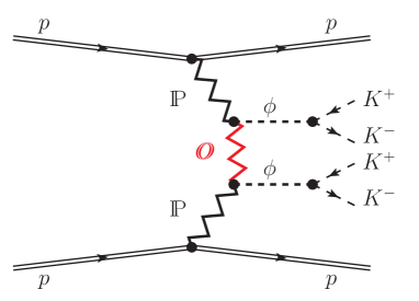
(a) (b)

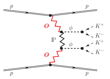
Figure 2: The Born-level diagrams for diffractive production of a $\phi$-meson pair with one and two odderon exchanges.

The diffractive production of two $\phi$ mesons seems to offer a good possibility to identify and/or study the odderon exchanges Ewerz:2003xi . At high energy there are two types of processes represented by the diagrams in Fig. 2. So far these processes have not yet been calculated or even estimated. A particularly important case worthy of attention is diagram (a) in Fig. 2. The advantage of this process compared to that in diagram (b) is that in diagram (a) no odderon-proton vertex is involved. Because the coupling of the odderon to the proton is probably small, one could expect $\sigma^{(\mathbb{O}-\mathbb{P}-\mathbb{O})}\ll\sigma^{(\mathbb{P}-\mathbb{O}-\mathbb{P})}$. Therefore, in the following we neglect the contribution with two odderon exchanges in the calculation.

The amplitude for the process shown by diagram (a) in Fig. 2 has the same form as the amplitude with the $\phi$-meson exchange discussed in Sec. III.1; see Eqs. (15)–(17). But here we have to make the following replacements:

$$i\Delta^{(\phi)}_{\mu\nu}(\hat{p})\to i\Delta^{(\mathbb{O})}_{\mu\nu}(s_{34},\hat{p}^{2})\,,$$ (52)

$$i\Gamma^{(\mathbb{P}\phi\phi)}_{\mu\nu\kappa\lambda}(k^{\prime},k)\to i\Gamma^{(\mathbb{P}\mathbb{O}\phi)}_{\mu\nu\kappa\lambda}(k^{\prime},k)\,.$$ (53)

Our ansatz for the effective propagator of the $C=-1$ odderon follows (3.16) and (3.17) of Ewerz:2013kda ,

$$i\Delta^{(\mathbb{O})}_{\mu\nu}(s,t)=-ig_{\mu\nu}\frac{\eta_{\mathbb{O}}}{M_{0}^{2}}(-is\alpha^{\prime}_{\mathbb{O}})^{\alpha_{\mathbb{O}}(t)-1}\,,$$ (54)

$$\alpha_{\mathbb{O}}(t)=\alpha_{\mathbb{O}}(0)+\alpha^{\prime}_{\mathbb{O}}\,t\,,$$ (55)

where in (54) we have $M_{0}^{-2}=1$ (GeV)^-2 for dimensional reasons. Furthermore, $\eta_{\mathbb{O}}$ is a parameter with value $\pm 1$ and $\alpha_{\mathbb{O}}(t)$ is the odderon trajectory, assumed to be linear in $t$. We choose, as an example, the slope parameter for the odderon the same as for the pomeron in (20). For the odderon intercept we choose a number of representative values. That is, we shall show results for

$$\eta_{\mathbb{O}}=\pm 1\,,\;\;\alpha^{\prime}_{\mathbb{O}}=0.25\;{\rm GeV}^{-2}\,,\;\;\alpha_{\mathbb{O}}(0)=1.05,\,1.00,\,0.95\,.$$ (56)

The odderon-exchange diagram presented in Fig. 2 (a), due to the Regge-based parametrisation with the odderon intercept $\alpha_{\mathbb{O}}(0)\sim 1.0$, should be especially relevant in the region of large rapidity separation of the $\phi$ mesons and large $\phi\phi$ invariant masses. This will be discussed further in Sec. IV.3.

For the $\mathbb{P}\mathbb{O}\phi$ vertex we use an ansatz analogous to the $\mathbb{P}\rho\rho$ vertex; see (3.47) of Ewerz:2013kda . We get then, orienting the momenta of the $\mathbb{O}$ and the $\phi$ outwards as shown in Fig. 3 (a), the following formula:

$$i\Gamma^{(\mathbb{P}\mathbb{O}\phi)}_{\mu\nu\kappa\lambda}(k^{\prime},k)=iF^{(\mathbb{P}\mathbb{O}\phi)}((k+k^{\prime})^{2},k^{\prime 2},k^{2})\left[2\,a_{\mathbb{P}\mathbb{O}\phi}\,\Gamma^{(0)}_{\mu\nu\kappa\lambda}(k^{\prime},k)-b_{\mathbb{P}\mathbb{O}\phi}\,\Gamma^{(2)}_{\mu\nu\kappa\lambda}(k^{\prime},k)\right].\qquad$$ (57)

Here $k^{\prime},\mu$ and $k,\nu$ are the momentum and vector index of the odderon and the $\phi$, respectively; $a_{\mathbb{P}\mathbb{O}\phi}$ and $b_{\mathbb{P}\mathbb{O}\phi}$ are (unknown) coupling constants; and $F^{(\mathbb{P}\mathbb{O}\phi)}\left((k+k^{\prime})^{2},k^{\prime 2},k^{2}\right)$ is a form factor. In practical calculations we take the factorized form for the $\mathbb{P}\mathbb{O}\phi$ form factor,

$$F^{(\mathbb{P}\mathbb{O}\phi)}((k+k^{\prime})^{2},k^{\prime 2},k^{2})=F((k+k^{\prime})^{2})\,F(k^{\prime 2})\,F^{(\mathbb{P}\mathbb{O}\phi)}(k^{2})\,,$$ (58)

where we adopt the monopole form

$$F(k^{2})=\frac{1}{1-k^{2}/\Lambda^{2}}\,,$$ (59)

and $F^{(\mathbb{P}\mathbb{O}\phi)}(k^{2})$ is a form factor normalised to $F^{(\mathbb{P}\mathbb{O}\phi)}(m_{\phi}^{2})=1$. The coupling parameters $a_{\mathbb{P}\mathbb{O}\phi}$, $b_{\mathbb{P}\mathbb{O}\phi}$ in (57) and the cutoff parameter $\Lambda^{2}$ in the form factor (59) could be adjusted to experimental data.

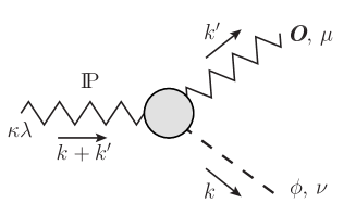
(a) (b)

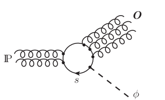
Figure 3: (a) Generic diagram for the $\mathbb{P}\mathbb{O}\phi$ vertex with momentum and Lorentz-indices assignments. (b) A QCD diagram contributing to the $\mathbb{P}\mathbb{O}\phi$ vertex.

In Fig. 3 (b) we show a QCD diagram which will contribute to the $\mathbb{P}\mathbb{O}\phi$ vertex. The “normal” decay of a $\phi$ meson from the QCD point of view is to three gluons produced in the annihilation of the $s\bar{s}$ quarks. A higher order correction can involve a five-gluon decay. Turning such a diagram around we arrive at the $\mathbb{P}\mathbb{O}\phi$ coupling shown in Fig. 3 (b).

For the considered reaction $pp\to pp\phi\phi$, the $\phi\phi$ subsystem energy $\sqrt{s_{34}}={\rm M}_{\phi\phi}$ is not very high and at threshold starts from $\sqrt{s_{34}}=2m_{\phi}$. The odderon-exchange amplitude applies for larger, certainly not too small, $\sqrt{s_{34}}$. At low energies the Regge type of interaction is not realistic and should be switched off. To achieve this requirement we shall multiply the odderon-exchange amplitude by a simple, purely phenomenological factor:

$$F_{{\rm thr}}(s_{34})=1-\exp\left(\frac{s_{{\rm thr}}-s_{34}}{s_{{\rm thr}}}\right)\,,$$ (60)

with $s_{{\rm thr}}=4m_{\phi}^{2}$. Our prescription leads to ${\cal M}^{(\mathbb{O}{\rm-exchange})}_{pp\to pp\phi\phi}\to 0$ when $s_{34}\to s_{{\rm thr}}$. The form factors of Eqs. (58) and (59) then guarantee that in our calculation the odderon only contributes in the Regge regime $|\hat{p}^{2}|\ll s_{34}$.

III.5 $\gamma$-exchange mechanism

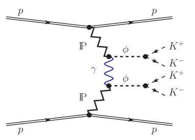
Figure 4: The Born-level diagram for diffractive production of a $\phi$-meson pair with an intermediate photon exchange.

The amplitude for the process shown by the diagram in Fig. 4 has the same form as the amplitude with the $\phi$-meson exchange discussed in Sec. III.1; see Eqs. (26) and (27). But we have to make the following replacements:

$$\Delta^{(\phi)}_{\rho_{1}\rho_{2}}(\hat{p})\to\Delta^{(\gamma)}_{\rho_{1}\rho_{2}}(\hat{p})=-\frac{g_{\rho_{1}\rho_{2}}}{\hat{p}^{2}}\,,$$ (61)

$$\hat{F}_{\phi}(\hat{p}^{2})\to\hat{F}_{\gamma}(\hat{p}^{2})\,,$$ (62)

where we assume that $\hat{F}_{\gamma}(\hat{p}^{2})=F_{M}(\hat{p}^{2})$ (25) and $\Lambda_{0}^{2}=1.0$ GeV², and

$$a_{\mathbb{P}\phi\phi}\to a_{\mathbb{P}\gamma\phi}=\frac{e}{\gamma_{\phi}}\,a_{\mathbb{P}\phi\phi}\,,$$ (63)

$$b_{\mathbb{P}\phi\phi}\to b_{\mathbb{P}\gamma\phi}=\frac{e}{\gamma_{\phi}}\,b_{\mathbb{P}\phi\phi}\,,$$ (64)

where $e>0,\gamma_{\phi}<0$, and $\gamma_{\phi}^{2}=4\pi/0.0716$ [see Eq. (5.3) of Donnachie:2002en and Eqs. (3.23)–(3.25) and Sec. 4 of Ewerz:2013kda ].

IV Results

In this section we wish to present first results for the $pp\to ppK^{+}K^{-}K^{+}K^{-}$ reaction via the intermediate $\phi(1020)\phi(1020)$ state corresponding to the diagrams shown in Figs. 1–4. In practice we work with the amplitudes in high-energy approximation; see (26) and (43).

IV.1 Comparison with the WA102 data

It was noticed in Barberis:1998bq that the cross section for the production of a $\phi\phi$ system, for the same interval of $|x_{F,\phi\phi}|\leqslant 0.2$, is almost independent of the center-of-mass energy. The experimental results are $\sigma_{{\rm exp}}^{(\phi\phi)}=42\pm 9$ nb at $\sqrt{s}=12.7$ GeV Armstrong:1986ky , $\sigma_{{\rm exp}}^{(\phi\phi)}=36\pm 6$ nb at $\sqrt{s}=23.8$ GeV Armstrong:1989hz , and $\sigma_{{\rm exp}}^{(\phi\phi)}=41.0\pm 3.7$ nb at $\sqrt{s}=29.1$ GeV Barberis:1998bq . This suggests that the double-pomeron-exchange mechanism shown in Fig. 1 is the dominant one for the $pp\to pp\phi\phi$ reaction in the above energy range. In the following we neglect, therefore, secondary reggeon exchanges.

In principle, there are many possible resonances with $J^{PC}=0^{++},0^{-+},2^{++}$ that may contribute to the $pp\to pp\phi\phi$ reaction represented by the diagram (b) in Fig. 1; see the fifth column in Table 1. Therefore, before comparing with the experimental data, let us first concentrate on the general characteristics of resonant production via the pomeron-pomeron fusion. We shall consider only three resonances as representative examples: $f_{0}(2100)$, $\eta(2225)$, and $f_{2}(2340)$. For illustration, in Fig. 5 we present the shape of distributions in $\rm{dP_{t}}$ and $\phi_{pp}$ for the experimental conditions as in the WA102 experiment Barberis:1998bq , that is, for $\sqrt{s}=29.1$ GeV and $|x_{F,\phi\phi}|\leqslant 0.2$. Here $\rm{dP_{t}}$ is the “glueball-filter variable”

$$\mbox{\boldmath$dP_{t}$}=\mbox{\boldmath$q_{t,1}$}-\mbox{\boldmath$q_{t,2}$}=\mbox{\boldmath$p_{t,2}$}-\mbox{\boldmath$p_{t,1}$}\,,\quad\rm{dP_{t}}=|\mbox{\boldmath$dP_{t}$}|\,,$$ (65)

and $\phi_{pp}$ is the azimuthal angle between the transverse momentum vectors $p_{t,1}$, $p_{t,2}$ of the outgoing protons. The results without (the thin lines) and with (the thick lines) absorptive corrections are shown in Fig. 5. The differential distributions have been normalised to 1 nb for both cases, with and without absorptive corrections. We can conclude that only the scalar and tensor resonances have similar characteristics as the WA102 experimental distributions Barberis:1998bq shown in Fig. 9 below. In the following we will assume that the $f_{2}(2340)$ resonance dominates.

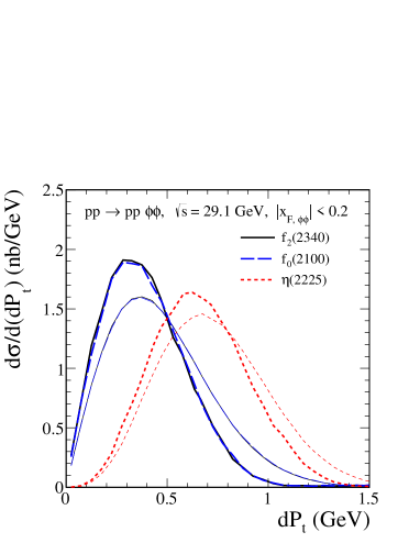
(a) (b)

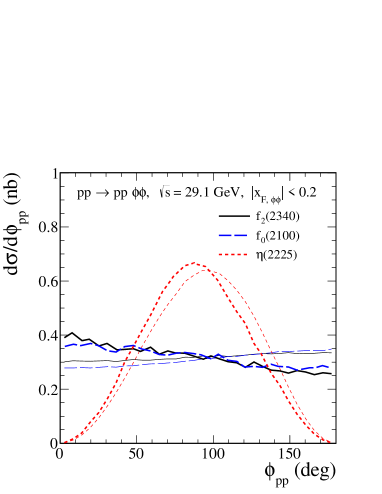
Figure 5: The distribution in $\rm{dP_{t}}$ (65) and in $\phi_{pp}$ for the central exclusive $\phi\phi$ production at $\sqrt{s}=29.1$ GeV and $|x_{F,\phi\phi}|\leqslant 0.2$. The results for scalar, pseudoscalar, and tensor resonances without (the thin lines) and with (the thick lines) absorptive corrections are shown. Because here we are interested only in the shape of the distributions, we normalised the differential distributions arbitrarily to 1 nb for both cases, with and without absorption corrections.

In Fig. 6 we show the results for the $\phi\phi$ continuum process via the $\phi$-meson exchange mechanism represented by diagram (a) in Fig. 1. In the left panel we present the $\phi\phi$ invariant mass distributions and in the right panel the distributions in $\rm{Y_{diff}}=\rm{Y}_{3}-\rm{Y}_{4}$. In our calculation we take $\Lambda_{off,E}=1.6$ GeV in (28) and the $\mathbb{P}\phi\phi$ coupling parameters from Lebiedowicz:2018eui . It is clearly seen from the left panel that the result without reggeization (see the green solid line) is well above the WA102 experimental data Barberis:1998bq ; Barberis:2000em normalised to the total cross section $\sigma_{{\rm exp}}^{(\phi\phi)}=41$ nb from Barberis:1998bq . The reggeization effect that leads to the suppression of the cross section should be applied here, but the way it should be included is less obvious. We show results for two prescriptions of reggeization given by Eqs. (30) and (34). We have checked that for the considered reaction $\langle-\hat{p}_{t}^{2}\rangle$, $\langle-\hat{p}_{u}^{2}\rangle\simeq 1$ GeV² (before reggeization). We have $s_{34}-4m_{\phi}^{2}>2$ GeV² for $\sqrt{s_{34}}={\rm M}_{\phi\phi}>2.5$ GeV. It can therefore be expected that the prescription (30) is relevant near threshold and especially for ${\rm M}_{\phi\phi}\gtrsim 3$ GeV. However, in the light of the discussion after Eq. (30) how to treat the low-${\rm M}_{\phi\phi}$ region, we consider also the alternative prescription (34) combined with (35). In this case we present predictions for ${\rm c_{y}}=1,1.5$, and 2 in (35). One can clearly see no effect of the reggeization at $\rm{Y_{diff}}=0$. The reggeization becomes more important when ${\rm M}_{\phi\phi}$ and $|{\rm Y_{diff}}|$ increase. For ${\rm c_{y}}=2$ and ${\rm M}_{\phi\phi}\gtrsim 3.5$ GeV we get similar results from (34) as from the first prescription (30).

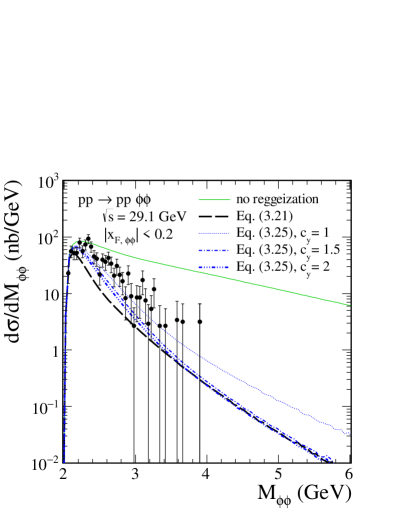
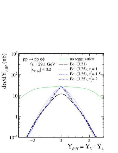
Figure 6: The distributions in $\phi\phi$ invariant mass (the left panel) and in $\rm{Y_{diff}}$, the rapidity distance between the two $\phi$ mesons (the right panel), for the $\phi$-exchange continuum contribution. The calculations were done for $\sqrt{s}=29.1$ GeV and $|x_{F,\phi\phi}|\leqslant 0.2$. In the left panel we show the WA102 experimental data Barberis:2000em normalised to the total cross section $\sigma_{{\rm exp}}^{(\phi\phi)}=41$ nb from Barberis:1998bq . The green solid line corresponds to the non-reggeized contribution. The results for the two prescriptions of reggeization, (30) and (34), are shown by the black and blue lines, respectively. The absorption effects are included here.

In Fig. 7 we compare our predictions including now the two mechanisms shown in Fig. 1 to the WA102 data Barberis:1998bq ; Barberis:2000em for the $\phi\phi$ invariant mass distribution from the $pp\to pp\phi\phi$ reaction. With our choice to keep only one $\mathbb{P}\mathbb{P}f_{2}$ coupling from (37), namely $g^{(1)}_{\mathbb{P}\mathbb{P}f_{2}}$, the distributions depend on the product of the couplings $g^{(1)}_{\mathbb{P}\mathbb{P}f_{2}}g^{\prime}_{f_{2}\phi\phi}$ and $g^{(1)}_{\mathbb{P}\mathbb{P}f_{2}}g^{\prime\prime}_{f_{2}\phi\phi}$ with $g^{\prime}_{f_{2}\phi\phi}$ and $g^{\prime\prime}_{f_{2}\phi\phi}$ given in (41). Again, for orientation purposes, we shall assume here and in the following that only either the first or the second of the above products of couplings is nonzero. In the parameter set A we choose $g^{(1)}_{\mathbb{P}\mathbb{P}f_{2}}g^{\prime}_{f_{2}\phi\phi}\neq 0$, and in set B we choose $g^{(1)}_{\mathbb{P}\mathbb{P}f_{2}}g^{\prime\prime}_{f_{2}\phi\phi}\neq 0$; see Table 2. Of course, once good measurements of all the relevant distributions of our reaction are available, one can try – as will be correct – to fit a linear combination of the above two coupling terms to the data. Thus, we show in Fig. 7 results for the two sets of parameters given in Table 2, set A [see panel (a)] and set B [see panel (b)]. The long-dashed lines represent results for the reggeized $\phi$-exchange contribution. The short-dashed lines represent results for the $f_{2}(2340)\to\phi\phi$ resonance contribution. The solid lines represent the coherent sum of both contributions. We found a rather good agreement near ${\rm M}_{\phi\phi}=2.3$ GeV, taking into account only the continuum and $f_{2}(2340)$ meson, although the possibility of an $f_{2}(2300)$ meson contribution cannot be ruled out. Our predictions indicate therefore that in such a case we are dealing rather with an upper limit of the cross section for the $f_{2}$-resonance term. We wish to point out here that the interference of the continuum and resonance contributions depends on subtle details (choice of the couplings for resonant term, phase interpolation for the continuum term).

By comparing the theoretical results and the differential cross sections obtained by the WA102 Collaboration we fixed the parameters of the off-shell $\hat{t}/\hat{u}$-channel $\phi$-meson form factor ($\Lambda_{off,E}$ in (28)) and the $\mathbb{P}\mathbb{P}f_{2}$ and $f_{2}\phi\phi$ couplings. For the convenience of the reader we have collected in Table 2 the default numerical values of the parameters of our model used in the calculations.

Table 2: Some parameters of our model. The columns indicate the equation numbers where the parameter is defined and their numerical values used in the calculations.

Parameters for	Equation	Value (Set A)	Value (Set B)
$\phi$-exchange mechanism
$a_{\mathbb{P}\phi\phi}$	(27); Sec. IV B of Lebiedowicz:2018eui	0.49 GeV-3	0.49 GeV-3
$b_{\mathbb{P}\phi\phi}$	(27); Sec. IV B of Lebiedowicz:2018eui	4.27 GeV-1	4.27 GeV-1
$\Lambda_{0}^{2}$	(25); Sec. IV B of Lebiedowicz:2018eui	1.0 GeV2	1.0 GeV2
$\Lambda_{off,E}$	(28)	1.6 GeV	1.6 GeV
$\mathbb{P}\mathbb{P}\to f_{2}(2340)\to\phi\phi$ mechanism
$g_{\mathbb{P}\mathbb{P}f_{2}}^{(1)}$ $g_{f_{2}\phi\phi}^{\prime}$	(37) et seq.; (41)	12.0	0.0
$g_{\mathbb{P}\mathbb{P}f_{2}}^{(1)}$ $g_{f_{2}\phi\phi}^{\prime\prime}$	(37) et seq.; (41)	0.0	7.0
$\tilde{\Lambda}_{0}^{2}$	(39)	1.0 GeV2	1.0 GeV2
$\Lambda_{f_{2}}$	(40)–(42)	1.0 GeV	1.0 GeV

It can be observed that the WA102 experimental point at ${\rm M}_{\phi\phi}\approx 2.2$ GeV is well above our theoretical result ($\phi$-exchange contribution) and it may signal the presence of the $f_{J}(2220)$ resonance. As was shown in Fig. 5, mesons with $J=0$ and $J=2$ have similar characteristics. Therefore, the answer to the question about the spin of $f_{J}(2220)$ cannot be easily given by studying the $\phi\phi$ decay channel. Our model calculation, including only two contributions, the reggeized $\phi(1020)$-meson exchange and the production via the intermediate $f_{2}(2340)$, describes the WA102 experimental data up to ${\rm M}_{\phi\phi}=2.5$ GeV reasonably well; see Fig. 7. We cannot exclude a small contribution of the $X(2500)$ meson which was seen in $J/\psi\to\gamma\phi\phi$ Ablikim:2016hlu . Including the other resonances will only be meaningful once experiments with better statistics become available. Hopefully this will be the case at the LHC. The behaviour at higher values of ${\rm M}_{\phi\phi}\gtrsim 2.5$ GeV will be further discussed in Sec. IV.3.

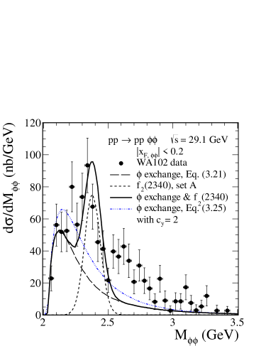
(a) (b)

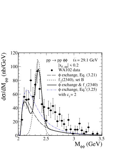
Figure 7: Invariant mass distributions for the central $\phi\phi$ system compared to the WA102 data Barberis:2000em at $\sqrt{s}=29.1$ GeV and $|x_{F,\phi\phi}|\leqslant 0.2$. The data points have been normalised to the total cross section $\sigma_{{\rm exp}}^{(\phi\phi)}=41$ nb from Barberis:1998bq . We show results for two sets of the parameters from Table 2, set A [see panel (a)] and set B [see panel (b)]. The black long-dashed line corresponds to the reggeized $\phi$-exchange contribution [Eq. (30)], while the black short-dashed line corresponds to the $f_{2}(2340)$ resonance term, and the black solid line represents the coherent sum of both contributions. For comparison, we show also the blue dashed-dotted line that corresponds to the reggeized $\phi$-exchange contribution using Eq. (34). The absorption effects are included here.

From Fig. 8 it is clearly seen that the shape of the $\rm{Y_{diff}}$ distribution is sensitive to the choice of the $f_{2}\phi\phi$ coupling (41) and of the reggeization ansatz. For the $\phi$ continuum process we show the results obtained for the two reggeization prescriptions, (30) and (34). Here $\rm{Y}_{3}$, $\rm{Y}_{4}$ are the rapidities of the two $\phi$ mesons. We show results in the $\phi\phi$ invariant mass window, ${\rm M}_{\phi\phi}\in(2.2,2.5)$ GeV, where tensor glueball candidates with masses around $2.3$ GeV are expected. Two sets of the parameters, set A and set B, from Table 2 give different results. It can, therefore, be expected that the $\rm{Y_{diff}}$ variable will be very helpful in determining the $f_{2}\phi\phi$ coupling using results expected from LHC measurements, in particular, if they cover a wider range of rapidities. This will be presented further in Figs. 13 and 14. We have checked that for the reaction $pp\to pp(\mathbb{P}\mathbb{P}\to f_{2}(2340)\to\phi\phi)$ discussed here the shapes of the $\rm{Y_{diff}}$ distributions do not depend significantly on the choice of the $\mathbb{P}\mathbb{P}f_{2}$ vertex coupling (37). This is a different situation compared to the one observed by us for the $pp\to pp(\mathbb{P}\mathbb{P}\to f_{2}(1270)\to\pi^{+}\pi^{-})$ reaction; see Figs. 7 and 8 of Lebiedowicz:2016ioh and Lebiedowicz:2019por .

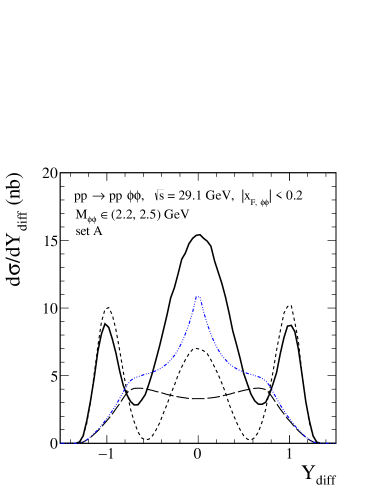
(a) (b)

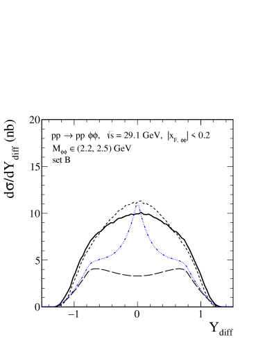
Figure 8: The distributions in rapidity distance between two centrally produced $\phi(1020)$ mesons $\rm{Y_{diff}}=\rm{Y}_{3}-\rm{Y}_{4}$ at $\sqrt{s}=29.1$ GeV for $|x_{F,\phi\phi}|\leqslant 0.2$ and ${\rm M}_{\phi\phi}\in(2.2,2.5)$ GeV. The meaning of the lines is the same as in Fig. 7. Here we show results for the two sets, A and B, of the parameters; see Table 2. The absorption effects are included here.

In Fig. 9 in the panels (a), (b), and (c) we compare our model results to the WA102 data on the differential distributions $d\sigma/d(\rm{dP_{t}})$, $d\sigma/d\phi_{pp}$, and $d\sigma/d|t|$ (that is $d\sigma/d|t_{1}|$ or $d\sigma/d|t_{2}|$), respectively. Here we used in the calculations the parameter set B of Table 2. We have checked that for these three observables the results obtained with the parameter set A of Table 2 are similar. The theoretical results correspond to the calculations including absorptive effects calculated at the amplitude level and related to the $pp$ nonperturbative interactions. Note that in the panels (a), (b), and (c) we also show the Born result for the $\phi$-exchange contribution. The ratio of full and Born cross sections $\langle S^{2}\rangle$ (the gap survival factor) at $\sqrt{s}=29.1$ GeV is $\langle S^{2}\rangle\cong 0.4$. From Figs. 5 and 9 we see the influence of absorption effects on the shape of distributions in $\phi_{pp}$ and $\rm{dP_{t}}$.

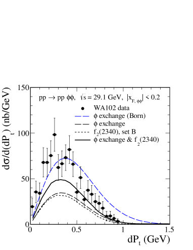
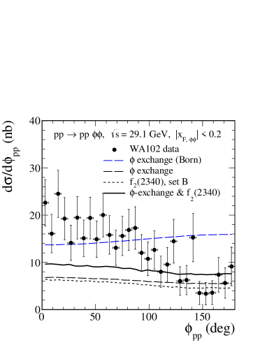
(a) (b) (c)

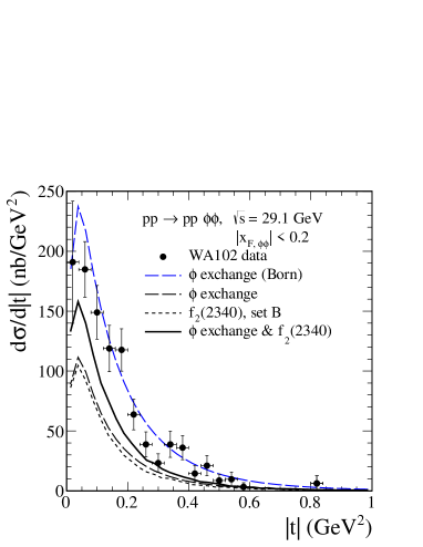
Figure 9: Differential cross sections for the central exclusive $\phi\phi$ production at $\sqrt{s}=29.1$ GeV and $|x_{F,\phi\phi}|\leqslant 0.2$. The data points from Barberis:1998bq have been normalised to the total cross section $\sigma_{{\rm exp}}^{(\phi\phi)}=41$ nb given there. The meaning of the lines is the same as in Fig. 7 (b) (set B). Here we show results for the $\phi$-exchange contribution using Eq. (30). The absorption effects are included, but, for comparison, we also show the reggeized $\phi$-exchange contribution in the Born approximation (without absorption effects) corresponding to the upper blue long-dashed line.

So far we have tried to adjust parameters of the continuum and the $f_{2}(2340)$ resonance terms in order not to exceed the WA102 experimental data for the $\phi\phi$ invariant mass distribution. We see that limiting to these mechanisms we cannot describe the data for ${\rm M}_{\phi\phi}>2.5$ GeV. In consequence we underestimate experimental distributions also in Fig. 9. Clearly, an additional mechanism is needed to resolve this problem. We shall discuss a possible solution of this problem in Sec. IV.3.

IV.2 Predictions for the LHC experiments

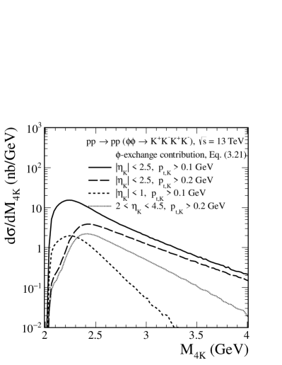
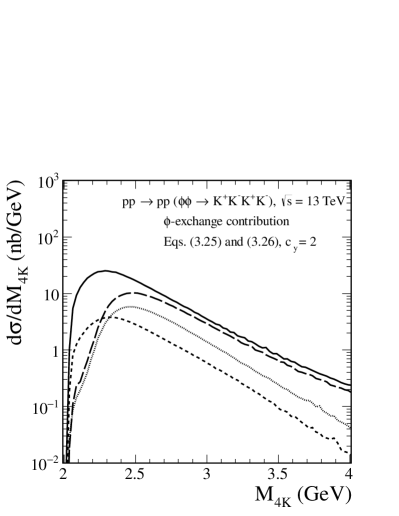
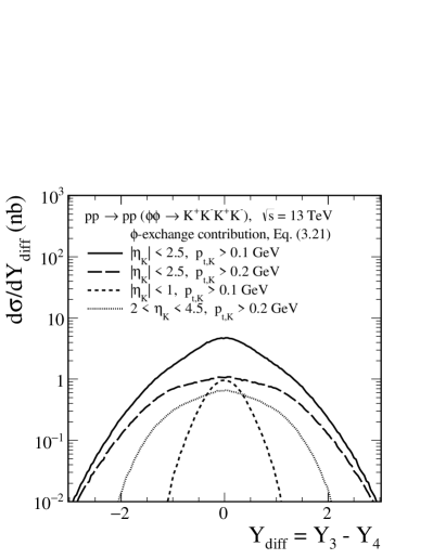
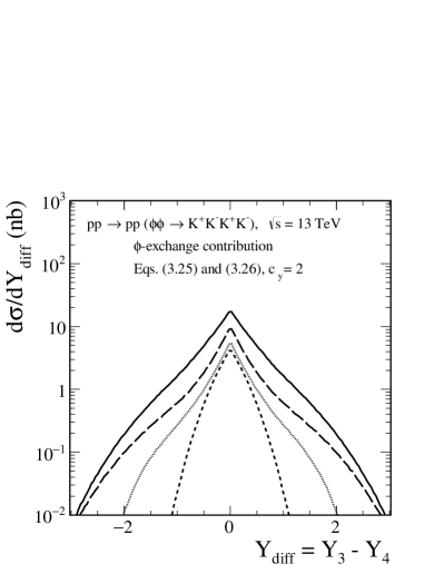
Figure 10: Differential cross sections as a function of the four-kaon invariant mass (top panels) and as function of $\rm{Y_{diff}}$ (bottom panels) for the $\phi$-exchange mechanism calculated for $\sqrt{s}=13$ TeV with the kinematical cuts specified in the figure legends. The results for the two prescriptions of reggeization (30) and (34) are presented. The absorption effects are included here.

We start from a discussion of the results for the $pp\to ppK^{+}K^{-}K^{+}K^{-}$ reaction obtained from the $\phi(1020)$-exchange mechanism discussed in Sec. III.1. The calculations were done for $\sqrt{s}=13$ TeV with typical experimental cuts on pseudorapidities and transverse momenta of centrally produced kaons. The ratio of the full and Born cross sections at $\sqrt{s}=13$ TeV is approximately $\langle S^{2}\rangle\cong 0.2$. In Fig. 10 we present the $K^{+}K^{-}K^{+}K^{-}$ invariant mass distributions (see the top panels) and the distributions in $\rm{Y_{diff}}=\rm{Y}_{3}-\rm{Y}_{4}$ (see the bottom panels) calculated for $\sqrt{s}=13$ TeV with the kinematical cuts specified in the figure legends. Here $\rm{Y}_{3}$ and $\rm{Y}_{4}$ mean $\rm{Y}_{K^{+}K^{-}}$ where the kaons are produced from the same $\phi$ meson decay. Of course, the larger the detector coverage in $\eta_{K}$, the larger becomes $|\rm{Y_{diff}}|$. In the calculations we take into account the intermediate $\phi$-meson reggeization. We show results for the two prescriptions of reggeization, (30) and (34), see the left and right panels, respectively. The results shown in the right panel were calculated with ${\rm c_{y}}=2$ in (35). We see that the choice of reggeization has a large impact on the results. The reggeization effect leads to a damping of the four-kaon invariant mass distributions. From the top panels, we see that increasing the $p_{t,K}$ cut from 0.1 GeV to 0.2 GeV significantly suppresses the cross section at small ${\rm M}_{4K}$. The first scenario of reggeization, Eq. (30), also significantly suppresses the region when $\rm{Y}_{3}\approx\rm{Y}_{4}$, that is, for $\rm{Y_{diff}}\simeq 0$. This is slightly different for the second reggeization scenario (34); see the bottom right panel. The cross section for the $\phi\phi$-continuum contribution is about 2 orders of magnitude smaller than the cross section for the $\rho\rho$-continuum contribution discussed in Lebiedowicz:2016zka .

In Fig. 11 we show further features of the ${\rm M}_{4K}$ and the $\rm{Y_{diff}}$ distributions for the $\phi$-exchange contribution. We show results for the reggeization prescription (30). The black solid line represents the complete result with the coherent sum of the $\hat{t}$- and $\hat{u}$-channel amplitudes; see Eqs. (16) and (17), respectively. The black long-dashed and blue short-dashed lines represent the results for their individual contributions, respectively. The black dotted line corresponds to the incoherent sum of $\hat{t}$ and $\hat{u}$ contributions. We can see that the complete result indicates a large interference effect between the $\hat{t}$- and $\hat{u}$-channel diagrams. This effect occurs in the region at low ${\rm M}_{4K}$ and $|\rm{Y_{diff}}|<1$. It can, therefore, be expected that the identification of diffractively produced high-mass resonances that decay into $\phi\phi$ pairs (e.g., $\eta_{c}$, $\chi_{c0}$, $\chi_{c2}$) should be possible at the LHC. For this purpose, one could study the distribution $d^{2}\sigma/d{\rm M}_{4K}d\mathrm{Y_{diff}}$ for the $pp\to ppK^{+}K^{-}K^{+}K^{-}$ reaction; see the discussion in Lebiedowicz:2018sdt for the $pp\to ppp\bar{p}$ reaction.

In Fig. 12 we show the distribution in $(\rm{Y_{diff}},{\rm M}_{4K})$ for the continuum $4K$ production via the reggeized $\phi$-exchange mechanism. In the left panel we show the results for (30) and in the right panel for (34) and (35) with ${\rm c_{y}}=2$. We note that with our prescriptions of reggeization and taking into account the kinematic cuts we have a clear correlation: large $|\rm{Y_{diff}}|$ automatically means large ${\rm M}_{4K}$. Basically this is due to the fact that the transverse momenta of the outgoing $\phi$ mesons stay rather small due to the form factors in (26). The behaviour of these distributions for large ${\rm M}_{4K}={\rm M}_{\phi\phi}$ can be understood as follows. We are in essence studying here the reaction $\mathbb{P}\mathbb{P}\to\phi\phi$ through $\phi$, respectively, for large ${\rm M}_{\phi\phi}$ $\phi_{\mathbb{R}}$ ($\phi$ reggeon) exchange. We expect then the maximum of this differential cross section for one $\phi$ forward and the other backward. This configuration corresponds to large ${\rm M}_{4K}$ and $|\rm{Y_{diff}}|$, giving the “ridge” in Fig. 12. In contrast, for ${\rm M}_{4K}$ near threshold the contributions from the $\hat{t}$ and $\hat{u}$ exchange diagrams overlap and interfere constructively; see Fig. 11. This effect gives the enhancement at small ${\rm M}_{4K}$ and small $|\rm{Y_{diff}}|$ in Fig. 12. Because of kinematic separation of the $\hat{t}$- and $\hat{u}$-channel continuum contributions for ${\rm M}_{4K}>3$ GeV the $\eta_{c}$ and $\chi_{c}$ mesons could be searched for preferentially at $\rm{Y_{diff}}=0$. If the reggeization ansatz (30) is close to what is realised in nature these resonances $\eta_{c}$, $\chi_{c}$ should be clearly visible at small $|\rm{Y_{diff}}|$. However, the reggeization ansatz (34) gives a larger continuum contribution at small $|\rm{Y_{diff}}|$; see also the lower panels of Fig. 10. Thus, if (34) is close to the truth, the identification of the above resonance contributions would be more difficult.

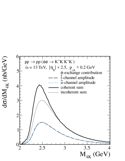
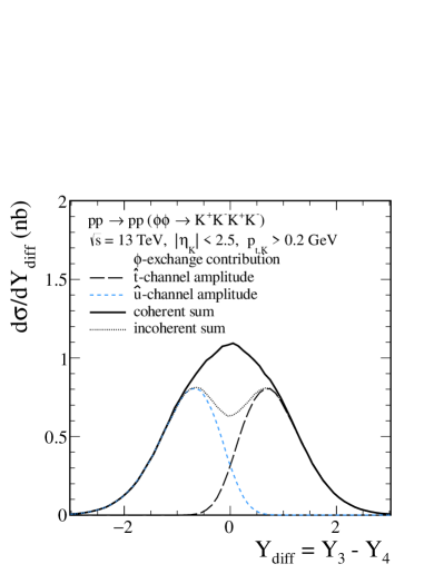
Figure 11: Differential cross sections as a function of the four-kaon invariant mass (left panel) and as a function of $\rm{Y_{diff}}$ (right panel) for the $pp\to pp(\phi\phi\to K^{+}K^{-}K^{+}K^{-})$ reaction calculated for $\sqrt{s}=13$ TeV and $|\eta_{K}|<2.5$, $p_{t,K}>0.2$ GeV. The results for the $\phi$-exchange contribution are presented. The black solid lines correspond to the coherent sum of the $\hat{t}$- and $\hat{u}$-channel amplitudes. Their incoherent sum is shown by the black dotted lines for comparison. The black long-dashed and blue short-dashed lines correspond to the results for the individual $\hat{t}$ and $\hat{u}$ terms, respectively. The absorption effects are included here.

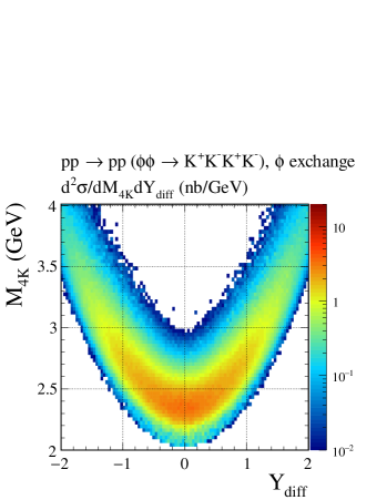
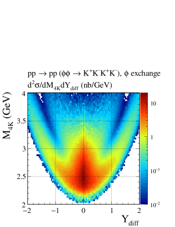
Figure 12: The two-dimensional distributions in $(\rm{Y_{diff}},{\rm M}_{4K})$ for the diffractive continuum four-kaon production for $\sqrt{s}=13$ TeV and $|\eta_{K}|<2.5$, $p_{t,K}>0.2$ GeV. The results for two prescriptions of reggeization are presented. The result in the left panel corresponds to the prescription (30), and the result in the right panel corresponds to Eqs. (34) and (35) for ${\rm c_{y}}=2$. The absorption effects are included here.

In Fig. 13 we present predictions for the $pp\to ppK^{+}K^{-}K^{+}K^{-}$ reaction including both the continuum $\phi$-exchange contribution and the $f_{2}(2340)$ contribution for two sets of the parameters fixed from the WA102 data; see Fig. 7 and Table 2. As can be clearly seen from Fig. 13, the resonance contribution generates, in both the ${\rm M}_{4K}$ and the $\rm{Y_{diff}}$ distributions, patterns with a complicated structure. In the calculations we include the $\phi$-exchange contribution using the reggeization prescription (30) and the dominant tensor $f_{2}(2340)$ resonance decaying into the $\phi\phi$ pair leading finally to the $K^{+}K^{-}K^{+}K^{-}$ final state. The resonance $f_{2}(2340)$ contribution is visible on top of the $\phi$-exchange continuum contribution. We can see that the complete result indicates a large interference effect of both terms. In principle, there may also be contributions from other tensor mesons and from $\eta$- and $f_{0}$-type mesons; see the fifth column in Table 1.

In Fig. 14 we show the distributions in $\rm{Y_{diff}}$ for different experimental conditions, $|\eta_{K}|<2.5$, $p_{t,K}>0.2$ GeV, $|\eta_{K}|<2.5$, $p_{t,K}>0.1$ GeV, $2.0<\eta_{K}<4.5$, $p_{t,K}>0.2$ GeV, from the top to bottom panels, respectively, and in the mass range ${\rm M}_{\phi\phi}\in(2.2,2.5)$ GeV. We show results for the two sets, A and B, of the parameters corresponding to the left and right panels. For the $\phi$-exchange contribution we show also results for the alternative prescription (34) and for ${\rm c_{y}}=2$ in (35). From Figs. 13 (bottom panels) and 14 we can see that the distribution in $\rm{Y_{diff}}$ can be used to determine the $f_{2}(2340)\to\phi\phi$ coupling (41), in particular, if low $p_{t,K}$ will be available.

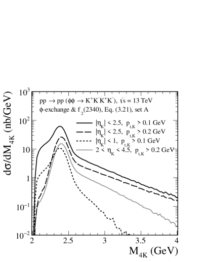
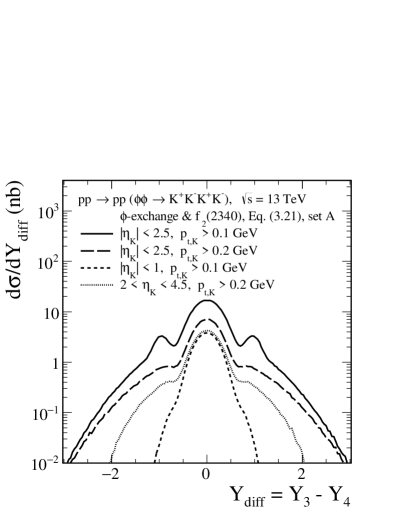
Figure 13: Differential cross sections as a function of the four-kaon invariant mass (top panels) and as a function of $\rm{Y_{diff}}$ (bottom panels) at $\sqrt{s}=13$ TeV for typical experimental cuts. The lines represent a coherent sum of the $\phi(1020)$-exchange and the $f_{2}(2340)$ terms. We show results for two sets of the parameters from Table 2, set A (see the left panels) and set B (see the right panels). The absorption effects are included here.

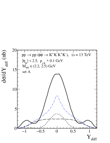
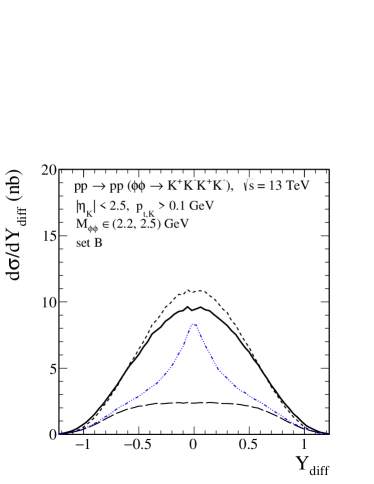
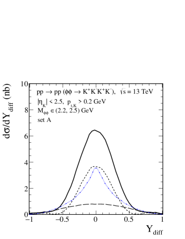
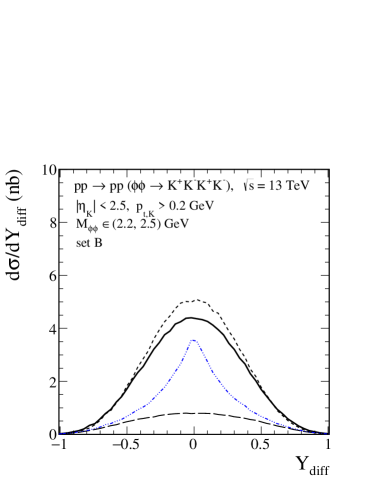
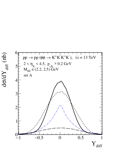
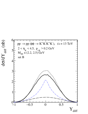
Figure 14: The distributions in $\rm{Y_{diff}}$ at $\sqrt{s}=13$ TeV for different experimental cuts on $\eta_{K}$ and $p_{t,K}$, and for ${\rm M}_{\phi\phi}\in(2.2,2.5)$ GeV. The meaning of the lines is the same as in Fig. 7. The absorption effects are included here.

In Fig. 15 we discuss the observables $\rm{dP_{t}}$ (65) and $\phi_{pp}$ for which the distributions are very sensitive to the absorption effects. The results shown correspond to $\sqrt{s}=13$ TeV and include cuts for $|\eta_{K}|<2.5$, $p_{t,K}>0.2$ GeV, and ${\rm M}_{4K}\in(2.2,2.5)$ GeV. Quite a different pattern can be seen for the Born case and for the case with absorption included. The absorptive corrections lead to significant modification of the shape of the $\phi_{pp}$ distribution and lead to an increase of the cross section for large $\rm{dP_{t}}$. This effect could be verified in future experiments when both protons are measured, e.g., by the CMS-TOTEM and the ATLAS-ALFA experimental groups.

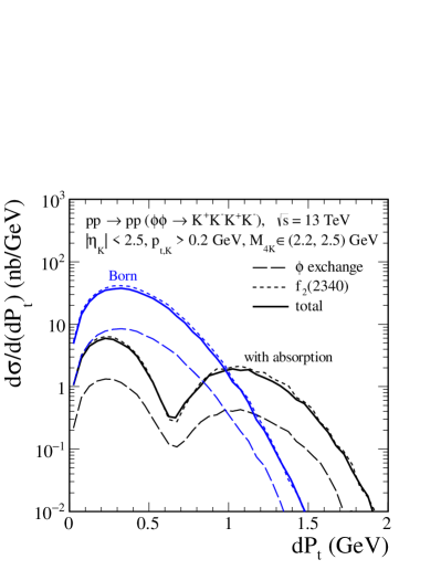
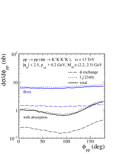
Figure 15: Distributions in $\rm{dP_{t}}$, the “glueball filter” variable (left panel), and in proton-proton relative azimuthal angle $\phi_{pp}$ (right panel) for the $pp\to pp(\phi\phi\to K^{+}K^{-}K^{+}K^{-})$ reaction through the $\phi$-exchange and $f_{2}(2340)$ mechanisms. Here the parameter set B from Table 2 and the reggeization formula (30) were used. The predictions shown correspond to $\sqrt{s}=13$ TeV and include cuts for $|\eta_{K}|<2.5$, $p_{t,K}>0.2$ GeV, and ${\rm M}_{4K}\in(2.2,2.5)$ GeV. The black lines correspond to the results with the absorption effects included. For comparison, the blue lines, marked “Born”, correspond to the results without absorption.

In Table 3 we have collected integrated cross sections in nb for different experimental cuts for the exclusive $K^{+}K^{-}K^{+}K^{-}$ production including only the contributions shown in Fig. 1. The results were obtained in the calculations with the tensor pomeron exchanges. The absorption effects are included in the calculations.

Table 3: The integrated cross sections in nb for the central exclusive $K^{+}K^{-}K^{+}K^{-}$ production in proton-proton collisions via the intermediate $\phi\phi$ system due to the mechanisms shown in Fig. 1. The results have been calculated for $\sqrt{s}=13$ TeV and some typical experimental cuts using the parameter set B from Table 2. The calculations for the $\phi$-exchange contribution were made using (30). The absorption effects are included here.

		Cross sections (nb)
$\sqrt{s}$, TeV	Cuts	Total	$\phi$ exchange	$f_{2}(2340)$
13	$|\eta_{K}|<1$, $p_{t,K}>0.1$ GeV	2.11	0.83	2.00
13	$|\eta_{K}|<2.5$, $p_{t,K}>0.1$ GeV	16.16	8.30	12.80
13	$|\eta_{K}|<2.5$, $p_{t,K}>0.2$ GeV	5.75	2.67	4.47
13	$2<\eta_{K}<4.5$, $p_{t,K}>0.2$ GeV	3.06	1.26	2.62

IV.3 Results including odderon exchange

In this section we shall discuss possibilities to observe odderon-exchange effects in the CEP of $\phi\phi$ pairs.

The odderon was introduced on theoretical grounds in Lukaszuk:1973nt ; Joynson:1975az . For a review of the odderon, see, e.g., Ewerz:2003xi . Recent experimental results by the TOTEM Collaboration Antchev:2017yns ; Antchev:2018rec have brought the odderon question to the forefront again. For recent theoretical papers dealing with the odderon, see, e.g., Ewerz:2013kda ; Bolz:2014mya , which came out before the TOTEM results, and Martynov:2017zjz ; Martynov:2018nyb ; Khoze:2017swe ; Broilo:2018qqs ; Goncalves:2018pbr ; Harland-Lang:2018ytk ; Csorgo:2018uyp .

Clearly, it is of great importance in this context to study possible odderon effects in reactions other than proton-proton elastic scattering. We shall argue here that the CEP of a $\phi\phi$ state offers a very nice way to look for odderon effects as suggested in Ewerz:2003xi .

In Figs. 16 and 17 we show results for the diffractive CEP of $\phi\phi$ pairs including the mechanism with odderon exchange shown in Fig. 2 (a). Here we take the following values of the parameters for the odderon exchange:

$$\eta_{\mathbb{O}}=\pm 1\,,\;\;\alpha_{\mathbb{O}}(0)=1.05\,,\;\;a_{\mathbb{P}\mathbb{O}\phi}=0\,,\;\;b_{\mathbb{P}\mathbb{O}\phi}=1.0,\,1.5\;{\rm GeV}^{-1}\,;$$ (66)

see (56), (57), and $\Lambda^{2}=1.0$ GeV² in (59). In the calculations we have used the parameter set B of Table 2 for the $\mathbb{P}\mathbb{P}f_{2}$ contribution. For the case of $\phi$ exchange we have used the formula of reggeization (30). In Fig. 16 we show the results for $\sqrt{s}=29.1$ GeV and compare them to the WA102 data. Figure 17 shows the predictions for $\sqrt{s}=13$ TeV using the same parameters. We show the $\phi$-meson-exchange contribution (see the black long-dashed line), the $f_{2}(2340)$ contribution (see the black dashed line), and the odderon-exchange contribution (see the red dotted line). The black dotted-dashed line corresponds to the photon-exchange contribution, represented by the diagram in Fig. 4, multiplied by a factor $10^{3}$ to be visible in the figure. The coherent sum of all contributions is shown by the red and blue solid lines, corresponding to $\eta_{\mathbb{O}}=-1$ and $\eta_{\mathbb{O}}=+1$, respectively. Clearly, the complete result indicates a large interference effect between the $\phi$- and odderon-exchange diagrams. We see from the right panel of Fig. 16 that for ${\rm M}_{\phi\phi}\gtrsim 2.5$ GeV the WA102 data leave room for a possible odderon contribution which here we normalised in such a way as not to exceed the WA102 cross section. Such an odderon contribution with $b_{\mathbb{P}\mathbb{O}\phi}=1.5$ GeV^-1 can be treated then rather as an upper limit. Of course the “true” odderon contribution may be much smaller.

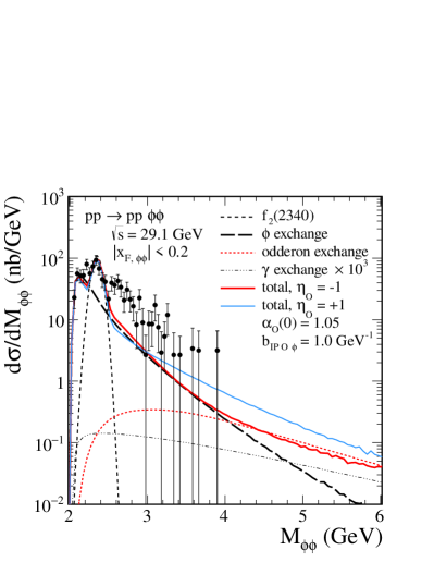
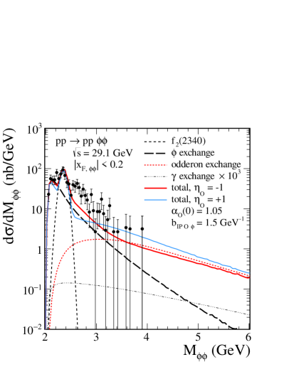
Figure 16: Invariant mass distributions for the central production of $\phi\phi$ at $\sqrt{s}=29.1$ GeV and $|x_{F,\phi\phi}|\leqslant 0.2$ together with the WA102 data Barberis:1998bq are shown. The black long-dashed line corresponds to the $\phi$-exchange contribution and the black dashed line corresponds to the $f_{2}(2340)$ contribution. The black dotted-dashed line corresponds to the $\gamma$-exchange contribution enlarged by a factor $10^{3}$. In the calculations the parameter set B of Table 2 for the $\phi$-exchange and $f_{2}$ terms, and the parameters (66) for the odderon term have been used. The red dotted line represents the odderon-exchange contribution for $a_{\mathbb{P}\mathbb{O}\phi}=0$, $b_{\mathbb{P}\mathbb{O}\phi}=1.0$ GeV^-1 (left panel) and for $a_{\mathbb{P}\mathbb{O}\phi}=0$, $b_{\mathbb{P}\mathbb{O}\phi}=1.5$ GeV^-1 (right panel). The coherent sum of all terms is shown by the red and blue solid lines for $\eta_{\mathbb{O}}=-1$ and $\eta_{\mathbb{O}}=+1$, respectively. Here we take $\alpha_{\mathbb{O}}(0)=1.05$. The absorption effects are included in the calculations.

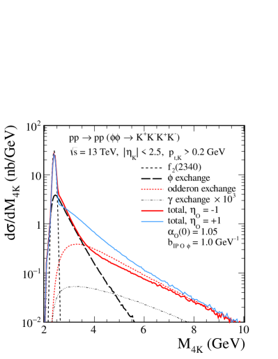
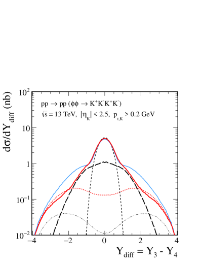
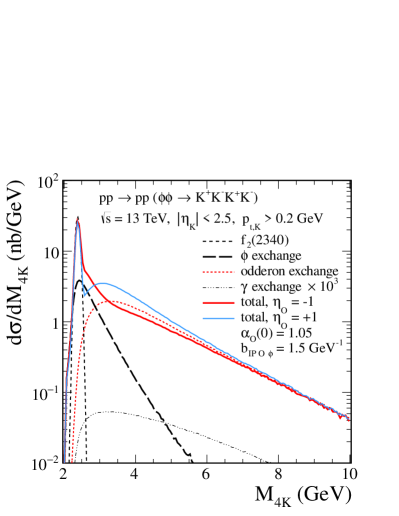
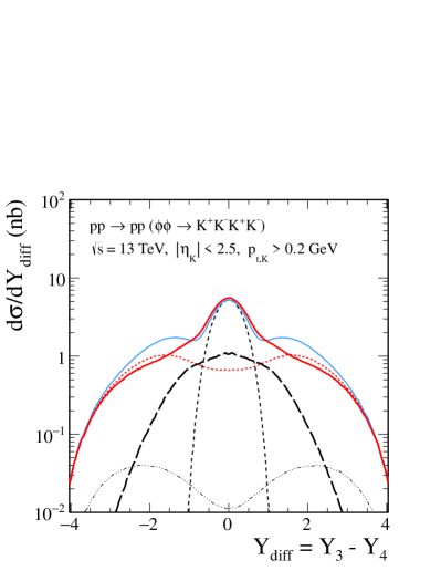
Figure 17: The distributions in ${\rm M}_{4K}$ (left panels) and in $\rm{Y_{diff}}$ (right panels) for the $pp\to pp(\phi\phi\to K^{+}K^{-}K^{+}K^{-})$ reaction calculated for $\sqrt{s}=13$ TeV and $|\eta_{K}|<2.5$, $p_{t,K}>0.2$ GeV. The meaning of the lines is the same as in Fig. 16. The red and blue solid lines correspond to the complete results with $\eta_{\mathbb{O}}=-1$ and $\eta_{\mathbb{O}}=+1$, respectively. The results for $b_{\mathbb{P}\mathbb{O}\phi}=1.0$ GeV^-1 (top panels) and for $b_{\mathbb{P}\mathbb{O}\phi}=1.5$ GeV^-1 (bottom panels) are presented. The absorption effects are included in the calculations.

In Fig. 17 we show the results for the ATLAS experimental conditions ($|\eta_{K}|<2.5$, $p_{t,K}>0.2$ GeV). For the odderon term we take here again the parameters (66). With these the odderon term gives a large enhancement of the ${\rm M}_{4K}$ distribution for ${\rm M}_{4K}\gtrsim 3$ GeV and clearly dominates at large $|\rm{Y_{diff}}|$. Whereas for ${\rm M}_{4K}\gtrsim 3$ GeV and $\eta_{\mathbb{O}}=+1$ there is constructive interference of the $\phi$-exchange and the odderon terms, for $\eta_{\mathbb{O}}=-1$ the interference is destructive. But in any case, for ${\rm M}_{4K}\gtrsim 4$ GeV and $|\rm{Y_{diff}}|\gtrsim 2$ the odderon term wins.

In Fig. 18 we show the complete result including the odderon exchange with $\eta_{\mathbb{O}}=-1$ and various values of the odderon intercept $\alpha_{\mathbb{O}}(0)$:

$$\eta_{\mathbb{O}}=-1\,,\;\;\alpha_{\mathbb{O}}(0)=0.95,\,1.00,\,1.05\,.$$ (67)

Even a much smaller odderon contribution should be visible for ${\rm M}_{4K}\gtrsim 5$ GeV and $|\rm{Y_{diff}}|>3$, provided the experimental statistics (luminosity) is sufficient. The distributions in ${\rm M}_{4K}$ and $\rm{Y_{diff}}$ seem therefore to offer good ways to identify the odderon exchange if it is there.

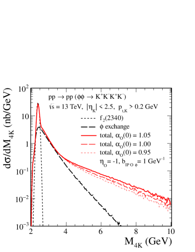
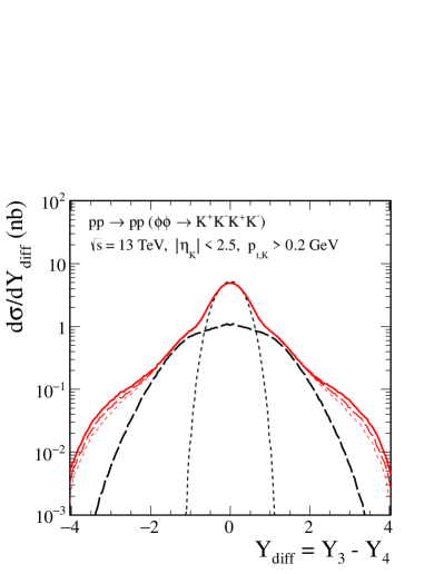
Figure 18: The complete results for $\sqrt{s}=13$ TeV and $|\eta_{K}|<2.5$, $p_{t,K}>0.2$ GeV are shown. Here we show results for $\eta_{\mathbb{O}}=-1$, $a_{\mathbb{P}\mathbb{O}\phi}=0$, $b_{\mathbb{P}\mathbb{O}\phi}=1$ GeV^-1, and for various values of the odderon intercept $\alpha_{\mathbb{O}}(0)$.

The small intercept of the $\phi$ reggeon exchange, $\alpha_{\phi}(0)=0.1$ Collins:1977 makes the $\phi$-exchange contribution steeply falling with increasing ${\rm M}_{4K}$ and $|\rm{Y_{diff}}|$. Therefore, an odderon with an intercept $\alpha_{\mathbb{O}}(0)$ around 1.0 should be clearly visible in these distributions if the $\mathbb{P}\mathbb{O}\phi$ coupling is of reasonable size. This is, at least, the conclusion of our present model study. Of course, in a real experiment many investigations of the background will be necessary before one could claim to have seen odderon exchange. Sources of background are $\phi_{\mathbb{R}}$ reggeon exchange as discussed in the present paper. But one will also have to consider $\omega_{\mathbb{R}}$ reggeon exchange and double $\phi$ production from two independent exchanges as shown in Fig. 19.

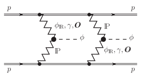
Figure 19: Example of a diagram for the production of two $\phi$ mesons by two independent exchanges.

V Conclusions

In the present paper we have presented first estimates of the contributions to the reaction $pp\to ppK^{+}K^{-}K^{+}K^{-}$ via the intermediate $\phi(1020)\phi(1020)$ resonance pairs. This reaction is being analyzed experimentally by the ALICE, ATLAS, CMS, and LHCb collaborations. The analysis of the reaction $pp\to pp(\mathbb{P}\mathbb{P}\to f_{2}\to\phi\phi)$ can be used for an identification of the tensor meson states. We note that the states $f_{2}(2300)$ and $f_{2}(2340)$ are good candidates for tensor glueballs.

We have considered the pomeron-pomeron fusion to $\phi\phi$ through the continuum process, with the $\hat{t}$- and $\hat{u}$-channel $\phi$-meson exchange, and through the $s$-channel resonance reaction [$\mathbb{P}\mathbb{P}\to f_{2}(2340)\to\phi\phi$]. The amplitudes for the process have been obtained within the tensor-pomeron approach Ewerz:2013kda . By comparing our theoretical results to the cross sections found by the WA102 Collaboration Barberis:1998bq ; Barberis:2000em , we have fixed some coupling parameters and the off-shell dependencies of the intermediate $\phi$ mesons. We have discussed also the $\phi\phi$ production through the $f_{0}(2100)$ and $\eta(2225)$ resonances, which were observed in radiative decays of $J/\psi$ Ablikim:2016hlu . We have shown that the contribution of the pseudoscalar $\eta(2225)$ meson is disfavored by the WA102 experimental distributions.

We have made estimates of the integrated cross sections as well as shown several differential distributions for different experimental conditions. The distribution in $\rm{Y_{diff}}$, the rapidity difference between the two $\phi$-mesons, depends strongly on the choice of the $f_{2}(2340)\to\phi\phi$ coupling. The general $f_{2}\phi\phi$ coupling is a sum of two basic couplings multiplied with two coupling constants; see (41). Our default values of the coupling parameters in the $\mathbb{P}\mathbb{P}f_{2}$ and $f_{2}\phi\phi$ vertices can be verified by future experimental results to be obtained at the LHC. Future studies at the LHC could potentially determine them separately. Low-$p_{t,K}$ cuts are required for this purpose. It has been shown that absorption effects change considerably the shapes of the “glueball-filter variable” distributions as well as those for the azimuthal angle between the outgoing protons.

The study of the $pp\to pp\phi\phi$ reaction offers the possibility to search for effects of the odderon. Such double diffractive production of two vector mesons with odderon exchange as a means to look for the latter was discussed in Ewerz:2003xi . In the present paper we have presented a concrete calculation of this process. Odderon contributions in diffractive production of single vector mesons, e.g., $pp\to pp\phi$, were investigated in Schafer:1991na . In the diffractive production of $\phi$ meson pairs, it is possible to have pomeron-pomeron fusion with intermediate $\hat{t}/\hat{u}$-channel $C=-1$ odderon exchange. The presence of odderon exchange in the middle of the diagram should be important and distinguishable from other contributions for relatively large rapidity separation between the $\phi$ mesons. Hence, to study this type of mechanism one should investigate events with rather large four-kaon invariant masses, outside of the region of resonances. These events are then “three-gap events”: proton–gap–$\phi$–gap–$\phi$–gap–proton. Experimentally, this should be a clear signature. A study of such events should allow a determination of the pomeron-odderon-$\phi$ meson coupling, or at least of an upper limit for it. Of course, one will have to investigate in detail the contribution of other exchanges like the $\phi_{\mathbb{R}}$ reggeon exchange studied in the present work. This could be done, for instance, by adjusting couplings and form factors at lower ${\rm M}_{\phi\phi}$ and then studying the extrapolations to higher ${\rm M}_{\phi\phi}$ where $\phi_{\mathbb{R}}$ exchange is a “background” to odderon exchange. Experimentally one has to make sure that one is really dealing with three-gap events. Thus, additional meson production in the gaps, a reducible background, must be excluded. There is, however, also the irreducible background from the production of two $\phi$ mesons by two independent exchanges; see Fig. 19. This has to be estimated theoretically and, in a sense, is an absorptive correction. If an odderon exchange is seen, then the distributions of the four-kaon invariant mass and of the rapidity difference between the two $\phi$ mesons will reveal the intercept of the odderon trajectory.

In conclusion we note the following. If the final protons in our reaction (10) can be measured one can reconstruct the complete kinematics of the reaction $\mathbb{P}+\mathbb{P}\to\phi+\phi$. A detailed study of this reaction as a function of its c.m. energy ${\rm M}_{\phi\phi}$ and its momentum transfer should then be possible. The great caveat is that one has to get the absorption corrections under good theoretical control. The resonances at low ${\rm M}_{\phi\phi}$ could then be investigated in detail. The special feature of the above reaction, however, is that the leading term at high energies must be due to a charge conjugation $C=-1$ exchange since $C=+1$ exchanges like the pomeron cannot contribute. Therefore, an odderon would give the leading term if its intercept is higher than that of the normal $C=-1$ reggeons. Clearly, an experimental study of CEP of a $\phi$-meson pair should be very valuable for clarifying the status of the odderon. Finally we note that analogous reactions which are suitable for odderon studies, see Ewerz:2003xi , are double $J/\psi$ and double $\Upsilon$ central exclusive production.

- (1) K. Akiba et al., (LHC Forward Physics Working Group), LHC forward physics, J. Phys. G43 (2016) 110201, arXiv:1611.05079 [hep-ph].
- (2) T. A. Aaltonen et al., (CDF Collaboration), Measurement of central exclusive production in collisions at and 1.96 TeV at CDF, Phys. Rev. D91 (2015) 091101, arXiv:1502.01391 [hep-ex].
- (3) V. Khachatryan et al., (CMS Collaboration), Exclusive and semi-exclusive production in proton-proton collisions at = 7 TeV, CMS-FSQ-12-004, CERN-EP-2016-261, arXiv:1706.08310 [hep-ex].
- (4) P. Lebiedowicz, O. Nachtmann, and A. Szczurek, Central exclusive diffractive production of the continuum, scalar and tensor resonances in and scattering within the tensor Pomeron approach, Phys. Rev. D93 (2016) 054015, arXiv:1601.04537 [hep-ph].
- (5) R. Schicker, (ALICE Collaboration), Central Diffraction in ALICE, arXiv:1205.2588 [hep-ex].
- (6) R. McNulty, Central Exclusive Production at LHCb, PoS DIS2016 (2016) 181.
- (7) R. Sikora, (STAR Collaboration), Recent results on Central Exclusive Production with the STAR detector at RHIC, arXiv:1811.03315 [hep-ex].
- (8) R. Staszewski, P. Lebiedowicz, M. Trzebiński, J. Chwastowski, and A. Szczurek, Exclusive Production at the LHC with Forward Proton Tagging, Acta Phys.Polon. B42 (2011) 1861–1870, arXiv:1104.3568 [hep-ex].
- (9) M. Albrow et al., (CMS, TOTEM Collaboration), CMS-TOTEM Precision Proton Spectrometer, CERN-LHCC-2014-021, TOTEM-TDR-003, CMS-TDR-13.
- (10) O. Nachtmann, Considerations concerning diffraction scattering in quantum chromodynamics, Annals Phys. 209 (1991) 436–478.
- (11) C. Ewerz, M. Maniatis, and O. Nachtmann, A Model for Soft High-Energy Scattering: Tensor Pomeron and Vector Odderon, Annals Phys. 342 (2014) 31–77, arXiv:1309.3478 [hep-ph].
- (12) C. Ewerz, P. Lebiedowicz, O. Nachtmann, and A. Szczurek, Helicity in Proton-Proton Elastic Scattering and the Spin Structure of the Pomeron, Phys. Lett. B763 (2016) 382, arXiv:1606.08067 [hep-ph].
- (13) L. Adamczyk et al., (STAR Collaboration), Single spin asymmetry in polarized proton-proton elastic scattering at GeV, Phys. Lett. B719 (2013) 62, arXiv:1206.1928 [nucl-ex].
- (14) P. Lebiedowicz, O. Nachtmann, and A. Szczurek, Exclusive central diffractive production of scalar and pseudoscalar mesons; tensorial vs. vectorial pomeron, Annals Phys. 344 (2014) 301–339, arXiv:1309.3913 [hep-ph].
- (15) A. Bolz, C. Ewerz, M. Maniatis, O. Nachtmann, M. Sauter, and A. Schöning, Photoproduction of pairs in a model with tensor-pomeron and vector-odderon exchange, JHEP 1501 (2015) 151, arXiv:1409.8483 [hep-ph].
- (16) P. Lebiedowicz, O. Nachtmann, and A. Szczurek, and Drell-Söding contributions to central exclusive production of pairs in proton-proton collisions at high energies, Phys. Rev. D91 (2015) 074023, arXiv:1412.3677 [hep-ph].
- (17) P. Lebiedowicz, O. Nachtmann, and A. Szczurek, Central production of in collisions with single proton diffractive dissociation at the LHC, Phys. Rev. D95 no. 3, (2017) 034036, arXiv:1612.06294 [hep-ph].
- (18) P. Lebiedowicz, O. Nachtmann, and A. Szczurek, Exclusive diffractive production of via the intermediate and states in proton-proton collisions within tensor pomeron approach, Phys. Rev. D94 no. 3, (2016) 034017, arXiv:1606.05126 [hep-ph].
- (19) P. Lebiedowicz, O. Nachtmann, and A. Szczurek, Central exclusive diffractive production of pairs in proton-proton collisions at high energies, Phys. Rev. D97 no. 9, (2018) 094027, arXiv:1801.03902 [hep-ph].
- (20) P. Lebiedowicz, O. Nachtmann, and A. Szczurek, Towards a complete study of central exclusive production of pairs in proton-proton collisions within the tensor Pomeron approach, Phys. Rev. D98 (2018) 014001, arXiv:1804.04706 [hep-ph].
- (21) P. Lebiedowicz, O. Nachtmann, and A. Szczurek, Extracting the pomeron-pomeron- coupling in the reaction through angular distributions of the pions, arXiv:1901.07788 [hep-ph].
- (22) F. E. Close and A. Kirk, Glueball - filter in central hadron production, Phys.Lett. B397 (1997) 333, arXiv:hep-ph/9701222 [hep-ph].
- (23) D. Barberis et al., (WA102 Collaboration), A kinematical selection of glueball candidates in central production, Phys.Lett. B397 (1997) 339.
- (24) D. Barberis et al., (WA102 Collaboration), A study of the centrally produced channel in interactions at 450 GeV/c, Phys. Lett. B413 (1997) 217, arXiv:9707021 [hep-ex].
- (25) D. Barberis et al., (WA102 Collaboration), A study of pseudoscalar states produced centrally in interactions at 450 GeV/, Phys. Lett. B427 (1998) 398, arXiv:hep-ex/9803029 [hep-ex].
- (26) D. Barberis et al., (WA102 Collaboration), A coupled channel analysis of the centrally produced and final states in interactions at 450 GeV/, Phys.Lett. B462 (1999) 462, arXiv:9907055 [hep-ex].
- (27) D. Barberis et al., (WA102 Collaboration), A study of the , , and observed in the centrally produced final states, Phys.Lett. B474 (2000) 423, arXiv:0001017 [hep-ex].
- (28) A. Kirk, Resonance production in central collisions at the CERN Omega spectrometer, Phys.Lett. B489 (2000) 29–37, arXiv:0008053 [hep-ph].
- (29) A. Kirk, A review of central production experiments at the CERN Omega spectrometer, Int. J. Mod. Phys. A29 no. 28, (2014) 1446001, arXiv:1408.1196 [hep-ex].
- (30) P. S. L. Booth et al., A high statistics study of the mass spectrum, Nucl. Phys. B273 (1986) 677.
- (31) P. S. L. Booth et al., Angular correlations in the system and evidence for hadronic production, Nucl. Phys. B273 (1986) 689.
- (32) A. Etkin, K. J. Foley, R. S. Longacre, W. A. Love, T. W. Morris, E. D. Platner, A. C. Saulys, S. J. Lindenbaum, C. S. Chan, and M. A. Kramer, Observation of three resonances in the glueball-enhanced channel , Phys. Lett. B165 (1985) 217.
- (33) A. Etkin et al., Increased statistics and observation of the , , and resonances in the Glueball enhanced channel , Phys. Lett. B201 (1988) 568.
- (34) D. Aston et al., Strangeonia and Kin: New Results from Kaon Hadroproduction with LASS, in Hadron ’89. Proceedings, 3rd International Conference on Hadron Spectroscopy, Ajaccio, France, September 23-27, 1989. 1989. http://www-public.slac.stanford.edu/sciDoc/docMeta.aspx?slacPubNumber=SLAC-PUB-5150.
- (35) D. Aston et al., Strangeonium production from LASS, Nucl. Phys. Proc. Suppl. 21 (1991) 5.
- (36) T. A. Armstrong et al., (ABBC Collaboration), Observation of double -meson production in the central region for the reactions and at 85 GeV/, Phys. Lett. 166B (1986) 245.
- (37) T. A. Armstrong et al., (WA76 Collaboration), Observation of double -meson production in the central region for the reaction at 300 GeV/, Phys. Lett. B221 (1989) 221.
- (38) D. Barberis et al., (WA102 Collaboration), A study of the centrally produced system in interactions at 450 GeV/, Phys. Lett. B432 (1998) 436, arXiv:hep-ex/9805018 [hep-ex].
- (39) C. Evangelista et al., (JETSET Collaboration), Study of the reaction from 1.1 to 2.0 GeV/, Phys. Rev. D57 (1998) 5370, arXiv:hep-ex/9802016 [hep-ex].
- (40) D. Bisello et al., (DM2 Collaboration), Search of Glueballs in the Decay, Phys. Lett. B179 (1986) 294.
- (41) Z. Bai et al., (MARK III Collaboration), Observation of a pseudoscalar state in near threshold, Phys. Rev. Lett. 65 (1990) 1309.
- (42) M. Ablikim et al., (BES Collaboration), Partial wave analysis of , Phys. Lett. B662 (2008) 330, arXiv:0801.3885 [hep-ex].
- (43) M. Ablikim et al., (BESIII Collaboration), Observation of pseudoscalar and tensor resonances in , Phys. Rev. D93 no. 11, (2016) 112011, arXiv:1602.01523 [hep-ex].
- (44) C. J. Morningstar and M. J. Peardon, Efficient glueball simulations on anisotropic lattices, Phys. Rev. D56 (1997) 4043, arXiv:hep-lat/9704011 [hep-lat].
- (45) C. J. Morningstar and M. J. Peardon, Glueball spectrum from an anisotropic lattice study, Phys.Rev. D60 (1999) 034509, arXiv:hep-lat/9901004 [hep-lat].
- (46) A. Hart and M. Teper, (UKQCD Collaboration), On the glueball spectrum in -improved lattice QCD, Phys. Rev. D65 (2002) 034502, arXiv:hep-lat/0108022 [hep-lat].
- (47) M. Loan, X.-Q. Luo, and Z.-H. Luo, Monte Carlo study of glueball masses in the Hamiltonian limit of SU(3) lattice gauge theory, Int. J. Mod. Phys. A21 (2006) 2905, arXiv:hep-lat/0503038 [hep-lat].
- (48) E. Gregory, A. Irving, B. Lucini, C. McNeile, A. Rago, C. Richards, and E. Rinaldi, Towards the glueball spectrum from unquenched lattice QCD, JHEP 10 (2012) 170, arXiv:1208.1858 [hep-lat].
- (49) Y. Chen et al., Glueball spectrum and matrix elements on anisotropic lattices, Phys. Rev. D73 (2006) 014516, arXiv:hep-lat/0510074 [hep-lat].
- (50) W. Sun, L.-C. Gui, Y. Chen, M. Gong, C. Liu, Y.-B. Liu, Z. Liu, J.-P. Ma, and J.-B. Zhang, Glueball spectrum from lattice QCD study on anisotropic lattices, Chin. Phys. C42 no. 9, (2018) 093103, arXiv:1702.08174 [hep-lat].
- (51) R. S. Longacre and S. J. Lindenbaum, Evidence for a fourth state related to the three , states explainable by glueball production, Phys. Rev. D70 (2004) 094041, arXiv:hep-ex/0407054 [hep-ex].
- (52) Y.-B. Yang, L.-C. Gui, Y. Chen, C. Liu, Y.-B. Liu, J.-P. Ma, and J.-B. Zhang, (CLQCD Collaboration), Lattice Study of Radiative Decay to a Tensor Glueball, Phys. Rev. Lett. 111 no. 9, (2013) 091601, arXiv:1304.3807 [hep-lat].
- (53) M. Ablikim et al., (BESIII Collaboration), Partial wave analysis of , Phys. Rev. D87 no. 9, (2013) 092009, arXiv:1301.0053 [hep-ex]. [Erratum: Phys. Rev.D87,no.11,119901(2013)].
- (54) M. Ablikim et al., (BESIII Collaboration), Amplitude analysis of the system produced in radiative decays, Phys. Rev. D98 no. 7, (2018) 072003, arXiv:1808.06946 [hep-ex].
- (55) M. Tanabashi et al., (Particle Data Group), Review of Particle Physics, Phys. Rev. D98 no. 3, (2018) 030001.
- (56) P. Lebiedowicz and A. Szczurek, Exclusive reaction: From the threshold to LHC, Phys.Rev. D81 (2010) 036003, arXiv:0912.0190 [hep-ph].
- (57) R. A. Kycia, J. Chwastowski, R. Staszewski, and J. Turnau, GenEx: A simple generator structure for exclusive processes in high energy collisions, Commun. Comput. Phys. 24 no. 3, (2018) 860, arXiv:1411.6035 [hep-ph].
- (58) R. A. Kycia, J. Turnau, J. J. Chwastowski, R. Staszewski, and M. Trzebiński, The adaptive Monte Carlo toolbox for phase space integration and generation, Commun. Comput. Phys. 25 (2019) 1547, arXiv:1711.06087 [hep-ph].
- (59) R. Kycia, P. Lebiedowicz, A. Szczurek, and J. Turnau, Triple Regge exchange mechanisms of four-pion continuum production in the reaction, Phys. Rev. D95 no. 9, (2017) 094020, arXiv:1702.07572 [hep-ph].
- (60) A. Donnachie and P. V. Landshoff, Total cross sections, Phys.Lett. B296 (1992) 227–232, arXiv:hep-ph/9209205 [hep-ph].
- (61) A. Donnachie, H. G. Dosch, P. V. Landshoff, and O. Nachtmann, Pomeron physics and QCD, Camb.Monogr.Part.Phys.Nucl.Phys.Cosmol. 19 (2002) 1–347.
- (62) M. Derrick et al., (ZEUS Collaboration), Measurement of elastic photoproduction at HERA, Phys. Lett. B377 (1996) 259, arXiv:hep-ex/9601009 [hep-ex].
- (63) J. Breitweg et al., (ZEUS Collaboration), Measurement of diffractive photoproduction of vector mesons at large momentum transfer at HERA, Eur. Phys. J. C14 (2000) 213, arXiv:hep-ex/9910038 [hep-ex].
- (64) P. D. B. Collins, An introduction to Regge theory and high energy physics. Cambridge University Press, 1977.
- (65) L. A. Harland-Lang, V. A. Khoze, and M. G. Ryskin, Modelling exclusive meson pair production at hadron colliders, Eur.Phys.J. C74 (2014) 2848, arXiv:1312.4553 [hep-ph].
- (66) C. Ewerz, The Odderon in Quantum Chromodynamics, arXiv:hep-ph/0306137 [hep-ph].
- (67) L. Łukaszuk and B. Nicolescu, A Possible interpretation of rising total cross-sections, Lett. Nuovo Cim. 8 (1973) 405.
- (68) D. Joynson, E. Leader, B. Nicolescu, and C. Lopez, Non-regge and hyper-regge effects in pion-nucleon charge exchange scattering at high energies, Nuovo Cim. A30 (1975) 345.
- (69) G. Antchev et al., (TOTEM Collaboration), First determination of the parameter at TeV - probing the existence of a colourless three-gluon bound state, CERN-EP-2017-335.
- (70) G. Antchev et al., (TOTEM Collaboration), Elastic differential cross-section at TeV and implications on the existence of a colourless 3-gluon bound state, CERN-EP-2018-341, TOTEM-2018-002, arXiv:1812.08610 [hep-ex].
- (71) E. Martynov and B. Nicolescu, Did TOTEM experiment discover the Odderon?, Phys. Lett. B778 (2018) 414, arXiv:1711.03288 [hep-ph].
- (72) E. Martynov and B. Nicolescu, Evidence for maximality of strong interactions from LHC forward data, Phys. Lett. B786 (2018) 207, arXiv:1804.10139 [hep-ph].
- (73) V. A. Khoze, A. D. Martin, and M. G. Ryskin, Elastic proton-proton scattering at 13 TeV, Phys. Rev. D97 no. 3, (2018) 034019, arXiv:1712.00325 [hep-ph].
- (74) M. Broilo, E. Luna, and M. Menon, Forward Elastic Scattering and Pomeron Models, Phys. Rev. D98 no. 7, (2018) 074006, arXiv:1807.10337 [hep-ph].
- (75) V. P. Goncalves, Searching the Odderon in the diffractive photoproduction at collisions, arXiv:1811.07622 [hep-ph].
- (76) L. A. Harland-Lang, V. A. Khoze, A. D. Martin, and M. G. Ryskin, Searching for the odderon in ultraperipheral proton-ion collisions at the LHC, Phys. Rev. D99 no. 3, (2019) 034011, arXiv:1811.12705 [hep-ph].
- (77) T. Csörgő, R. Pasechnik, and A. Ster, Odderon and proton substructure from a model-independent Lévy imaging of elastic and collisions, Eur. Phys. J. C79 no. 1, (2019) 62, arXiv:1807.02897 [hep-ph].
- (78) A. Schäfer, L. Mankiewicz, and O. Nachtmann, Double-diffractive and production as a probe for the odderon, Phys.Lett. B272 (1991) 419.