Terahertz continuum generation in the LCS lattice

Abstract

Rabi oscillations in two-level Dirac systems have been shown to alter the frequency content of the system’s nonlinear response. In particular, when considering Rabi oscillations in a quantum model beyond the semiclassical Boltzmann theory, even harmonics may be generated despite the centrosymmetric nature of these systems. This effect magnifies with increasing excitation intensity. In this work, we extend the Rabi theory to a three-level Dirac system arising from a line-centered-square optical lattice. In this case, the Dirac cones are bisected at the Dirac point by a flat band that persists throughout the Brillioun zone. Due to the presence of this flat band, we expect a significant enhancement of the coupling between Dirac states, resulting in a large increase of the Rabi effects and the associated nonlinearities, leading to continuum generation of terahertz radiation.

I INTRODUCTION

Due to the novel electronic Castro Neto et al. (2009), thermal Hu et al. (2009), mechanical Lee et al. (2008) and optoelectronic Nair et al. (2008) properties it possesses, graphene has drawn a considerable amount of attention in many fields. Its Dirac band structure contributes to the optical response of graphene, giving rise to novel effects including efficient light absorption and a large nonlinear susceptibility. The harmonic response of the current density in graphene, based on the semiclassical Boltzmann theory and the centrosymmetric structure of graphene itself, was believed to be restricted to only odd harmonic spectra. However, Lee et. al. Lee and Jiang (2014) demonstrated that even in the presence of the centrosymmetry, the nonlinear optical response in graphene is not limited to odd harmonic spectra when the electron dynamics of Rabi oscillations are included in the current response Tritschler et al. (2003). The Rabi oscillation can shift the current-induced harmonic spectra of graphene and thus lead to a peak at the spectral position of the second harmonic of the incident light.

The line-centered-square (LCS) lattice (Fig. 1(a)), formed by using ultracold atoms trapped in an optical lattice, was first described by Shen et. al. Shen et al. (2010). It is a two-dimensional counterpart of the face-centered-cubic lattice, and contains a single Dirac cone in the energy spectrum with an additional flat band energy state touching at the Dirac point. Thus, the LCS lattice exhibits three bands, i.e. the conduction band, the valence band and a central flat band (Fig. 1(b)). The band structure of the LCS lattice satisfies a three-component quantum equation for pseudospin 1 Fermions.

In this paper, we calculate the Rabi contribution to the harmonic spectra of massless Dirac fermions in LCS lattice for various parameter sets. Following Lee et. al. Lee and Jiang (2014), we begin with the time-dependent Dirac equation (TDDE) to model LCS electron dynamics. By transforming the TDDE to the dipole gauge (DG) Kobe (1982), we obtain the Rabi frequency of the LCS lattice, and use it to calculate the Rabi contribution to the current response. We demonstrate that, in analogy with graphene, the nonlinear optical response of LCS lattice is not restricted to odd harmonic spectra when Rabi oscillation contributes strongly to the current response. We find the first five orders of the harmonic spectra, ranging from 2 THz to 10 THz, fuse into a continuous spectrum in the presence of a 2 THz incident light field. Further, odd harmonics up to $n=25$ exhibit significant energy content for reasonable pump energy levels.

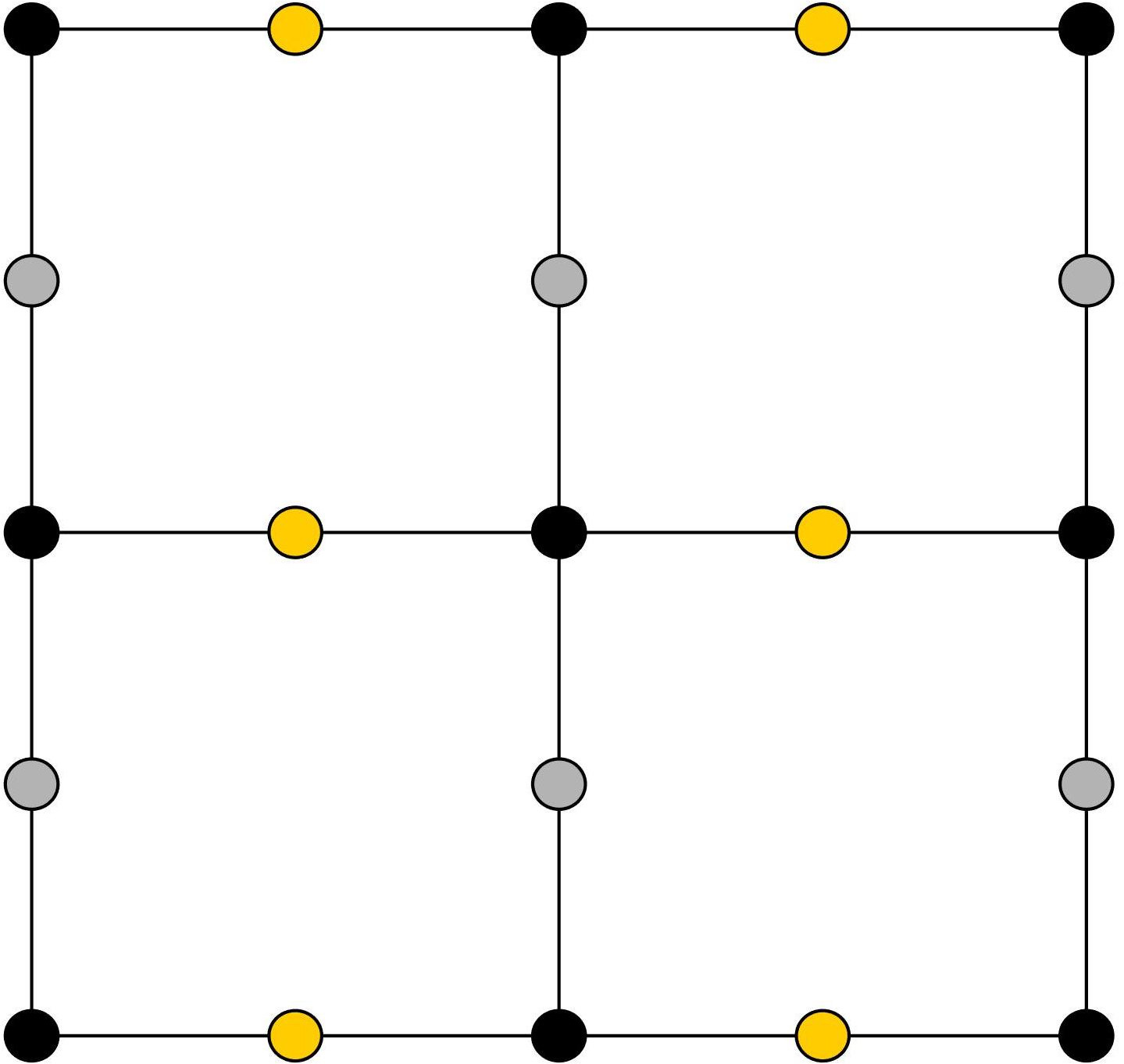
(a)

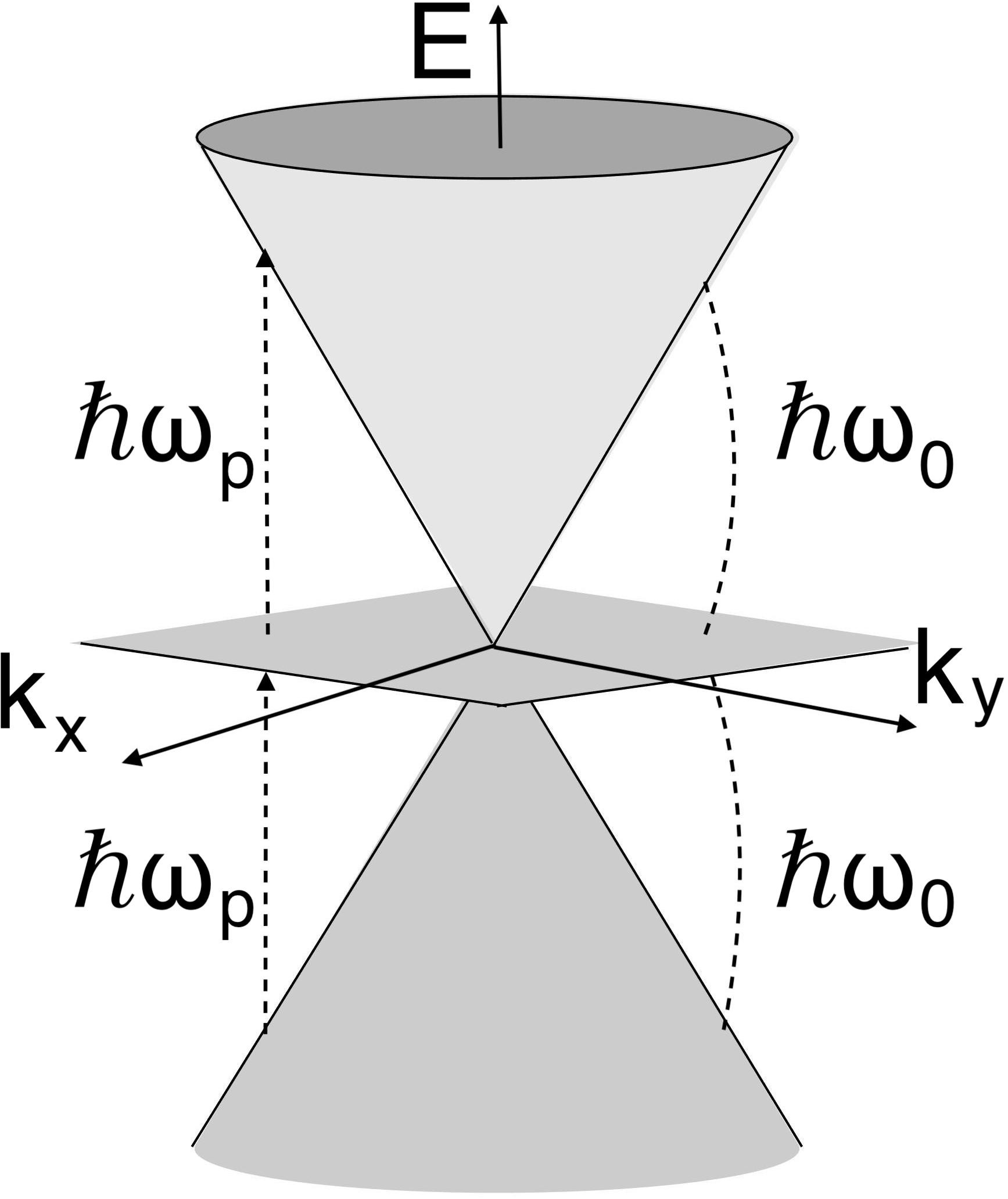
(b)

Figure 1: Schematic illustration of the LCS lattice (a) configuration and (b) energy band structure.

The paper is organized as follows. In Section II, we begin with the TDDE in the DG to obtain the Rabi frequency and current response of the LCS lattice due to the terahertz (THz) light field. In Section III, we elucidate the Rabi coupling effect on harmonic spectra. Finally, we draw conclusions in Section IV.

II THEORETICAL MODEL

II.1 Eigenstates of the unperturbed Hamiltonian

In the LCS lattice, the Dirac Hamiltonian of a 2D massless electron can be described Shen et al. (2010) as:

$$\mathbf{H}_{0}=\hbar v_{0}\begin{pmatrix}0&k_{x}&0\\ k_{x}&0&k_{y}\\ 0&k_{y}&0\end{pmatrix}$$ (1)

where $v_{0}=\pm ta/\hbar$ is the Fermi velocity, $a$ is the LCS lattice constant, $t$ is a hopping parameter, $k_{x}$ and $k_{y}$ are the perturbation components of ${\bf k}$ from Dirac point, and $k=|\bf k|$. The eigenstates of $\textit{H}_{0}$ are given by $\psi^{(i)}_{\bf k}({\bf r})=(1/2\pi)\,\exp(\textnormal{i}{\bf k}\cdot{\bf r})\,\mathbf{u}^{(i)}_{\bf k}$ with eigenvalues 0, $-\hbar v_{0}\sqrt[2]{{k_{x}}^{2}+{k_{y}}^{2}}$,and $\hbar v_{0}\sqrt{{k_{x}}^{2}+{k_{y}}^{2}}$, and eigenvectors:

$$\mathbf{u}^{(1)}_{\bf k}=\begin{bmatrix}-\frac{k_{y}}{k}\\ 0\\ \frac{k_{x}}{k}\end{bmatrix},\ \mathbf{u}^{(2)}_{\bf k}=\begin{bmatrix}\frac{k_{x}}{\sqrt{2}k}\\ -\frac{1}{\sqrt{2}}\\ \frac{k_{y}}{\sqrt{2}k}\end{bmatrix},\ \mathrm{and}\ \mathbf{u}^{(3)}_{\bf k}=\begin{bmatrix}\frac{k_{x}}{\sqrt{2}k}\\ \frac{1}{\sqrt{2}}\\ \frac{k_{y}}{\sqrt{2}k}\end{bmatrix}$$ (2)

The orthonormality of these eigenstates is given by $\int\textit{d}^{2}{\bf r}[\psi^{(s^{\prime})}_{\bf k^{\prime}}(\bf r)]^{\dagger}\psi^{(\textnormal{s})}_{\bf k}(\bf r)=\delta({\bf k}-{\bf k^{\prime}})\delta_{ss^{\prime}}$, with $s,s^{\prime}=1,2,3$ indexing the pseudospin. We also note here that the pseudospin indices 1, 2, and 3 correspond to the flat, valence, and conduction bands respectively.

II.2 TDDE in the dipole gauge with terahertz optical pump

We define the incident terahertz optical pump field in the Coulomb gauge by the vector potential:

$${\bf A}(t)=\frac{E_{0}}{\omega_{0}}e^{-\frac{1}{2}{\ln 2}(\frac{t}{\tau})^{2}}[\hat{x}{\cos(\frac{\zeta}{2})}{\cos(\omega_{0}t)}+\hat{y}{\sin(\frac{\zeta}{2})}{\sin(\omega_{0}t)}],$$ (3)

where $E_{0}$ is the peak of the incident electric-field strength, $\zeta$ is the polarization factor, $\omega_{0}=2\pi f_{0}$ is the central frequency and $\tau$ is the pulse width. With this incident light field, the Dirac Hamiltonian may be written:

$$\hat{H}={\textit{v}_{0}}{\bf J}\cdot({{\hbar}{\bf\hat{k}}+q{\bf A}(t)}),$$ (4)

where ${\bf J}=[{\bf{J_{3}}{S_{-}},{J_{3}}{S_{+}},0}]^{\dagger}$, ${\bf S_{\pm}}$ are the spin-1 ladder operators, $\hbar\hat{\mathbf{k}}$ is the momentum operator, and ${\bf J_{3}}$ is the $3\times 3$ exchange matrix. Using this Hamiltonian, we obtain the TDDE in the Coulomb gauge:

$$i\hbar\,\frac{\partial\Psi({\bf r},t)}{\partial t}=\hat{H}\,\Psi({\bf r},t)$$ (5)

For a normally-incident THz optical field, the solution to Eq. 5 may be expressed as:

$$\Psi({\bf r},t)=\Psi^{D}({\bf r},t)\exp\left[\left(-i\left(\frac{e}{\hbar}\right)\bf r\cdot A{\textnormal{(t)}}\right)\right]$$ (6)

This represents a gauge transformation from Coulomb to dipole gauge where $-i(\frac{e}{\hbar})\bf r\cdot A{\textnormal{(t)}}$ is the gauge generating function for the transformation, and $\Psi^{D}({\bf r},t)$ is the spinor wavefunction in the dipole gauge, which we expand in the eigenstates of $\mathbf{H}_{0}$ as:

$$\Psi^{D}({\bf r},t)=c_{1}(t)\psi^{(1)}_{\bf k}({\bf r})+c_{2}(t)\psi^{(2)}_{\bf k}({\bf r})+c_{3}(t)\psi^{(3)}_{\bf k}({\bf r})$$ (7)

Substituting $\Psi({\bf r},t)$ into Eq. 5 yields the TDDE in the dipole gauge:

$$i\hbar\,\frac{\partial\Psi^{D}({\bf r},t)}{\partial t}=[\mathbf{H}_{0}+\hat{V}(t)])\,\Psi^{D}({\bf r},t),$$ (8)

with $\hat{V}(t)=e{\bf r}\cdot{\bf E}(t){\textit{I}_{3}}$, where ${\bf E}(t)$ is the incident electric field and $\textit{I}_{3}$ is the 3x3 identity matrix. In our calculations, ${\bf E}(t)$ is assumed to be linearly polarized along $x$ axis; thus $\hat{V}(t)=q\,x\,E_{x}(t)\,\textit{I}_{3}$ and $\zeta=0$.

Substituting Eq.7 into Eq.8, premultiplying the result by $[\psi^{(1)}_{\bf k^{\prime}}({\bf r})]^{\dagger}$, and using the real-space orthogonality property of the eigenstates, we obtain:

$$i\hbar(2\pi)^{2}[\dot{c}_{1}(t)(\frac{k_{y}k_{y}^{\prime}}{kk^{\prime}}+\frac{k_{x}k_{x}^{\prime}}{kk^{\prime}})+\dot{c}_{2}(t)(\frac{k_{y}k_{x}^{\prime}}{\sqrt{2}kk^{\prime}}-\frac{k_{x}k_{y}^{\prime}}{\sqrt{2}kk^{\prime}})\\ +\dot{c}_{3}(t)(\frac{k_{y}k_{x}^{\prime}}{\sqrt{2}kk^{\prime}}-\frac{k_{x}k_{y}^{\prime}}{\sqrt{2}kk^{\prime}})]\delta({\bf k}-{\bf k^{\prime}})\\ =eE_{x}(t)\int xe^{i({\bf k}-{\bf k^{\prime}})\cdot{\bf r}}[c_{1}(t)(\frac{k_{y}k_{y}^{\prime}}{kk^{\prime}}+\frac{k_{x}k_{x}^{\prime}}{kk^{\prime}})\\ +c_{2}(t)(\frac{k_{y}k_{x}^{\prime}}{\sqrt{2}kk^{\prime}}-\frac{k_{x}k_{y}^{\prime}}{\sqrt{2}kk^{\prime}})+c_{3}(t)(\frac{k_{y}k_{x}^{\prime}}{\sqrt{2}kk^{\prime}}-\frac{k_{x}k_{y}^{\prime}}{\sqrt{2}kk^{\prime}})]d^{2}\bf r$$ (9)

Integrating Eq. 9 over the $\bf k^{\prime}$ space and using the transformations: $c_{1}(t)=\tilde{c}_{1}(t),\ c_{2}(t)=\tilde{c}_{2}(t)\exp(i\omega_{p}t),\ \mathrm{and}\ c_{3}(t)=\tilde{c}_{3}(t)\exp(-i\omega_{p}t)$ yields the equation of motion for $\dot{\tilde{c}}_{1}(t)$:

$$\dot{\tilde{c}}_{1}(t)=-\frac{eE_{x}(t)}{\sqrt{2}\hbar k^{2}}(\tilde{c}_{2}(t)\exp(i\omega_{p}t)+\tilde{c}_{3}(t)\exp(-i\omega_{p}t))k_{y}.$$ (10)

where $\omega_{p}=v_{0}k$ is the eigenfrequency.

Similarly, following the procedure above with $[\psi^{(2)}_{\bf k^{\prime}}({\bf r})]^{\dagger}$ and $[\psi^{(3)}_{\bf k^{\prime}}({\bf r})]^{\dagger}$ yields the following equations of motion for $\dot{\tilde{c}}_{2}(t)$ and $\dot{\tilde{c}}_{3}(t)$ respectively:

$$\dot{\tilde{c}}_{2}(t)=\frac{eE_{x}(t)}{\sqrt{2}\hbar k^{2}}\tilde{c}_{1}(t)\exp(-i\omega_{p}t)k_{y}.$$ (11)

$$\dot{\tilde{c}}_{3}(t)=\frac{eE_{x}(t)}{\sqrt{2}\hbar k^{2}}\tilde{c}_{1}(t)\exp(i\omega_{p}t)k_{y}.$$ (12)

Solving the coupled equations Eqs. 10, 11, and 12 numerically using a pulsed THz pump, we can observe the dynamical behavior of the system, including Rabi oscillations. To gain a detailed understanding of this behavior, we first consider resonant excitation with $k=\omega_{0}/v_{0}$, directional angle of momentum $\phi_{p}=\pi/4$, and light field intensity $I=1kW/cm^{2}$. We assume that the electron population is initially in the valence band. Pump parameters $f_{0}=2$ THz and $\tau=1$ ps are used in our calculations. Fig. 2 shows the temporal evolution of the normalized band populations $|c_{1}(t)|^{2}$, $|c_{2}(t)|^{2}$ and $|c_{3}(t)|^{2}$ for this configuration. With this parameter set, the Rabi frequency of the central flat band is nearly double that of the valence and conduction band, and the Rabi frequencies of valence and conductions are nearly the same. In addition to the Rabi oscillation, there is a high-frequency oscillation component observed. This component arises due to the counter-rotating wave oscillating at $(\omega_{0}+2\omega_{p})$.

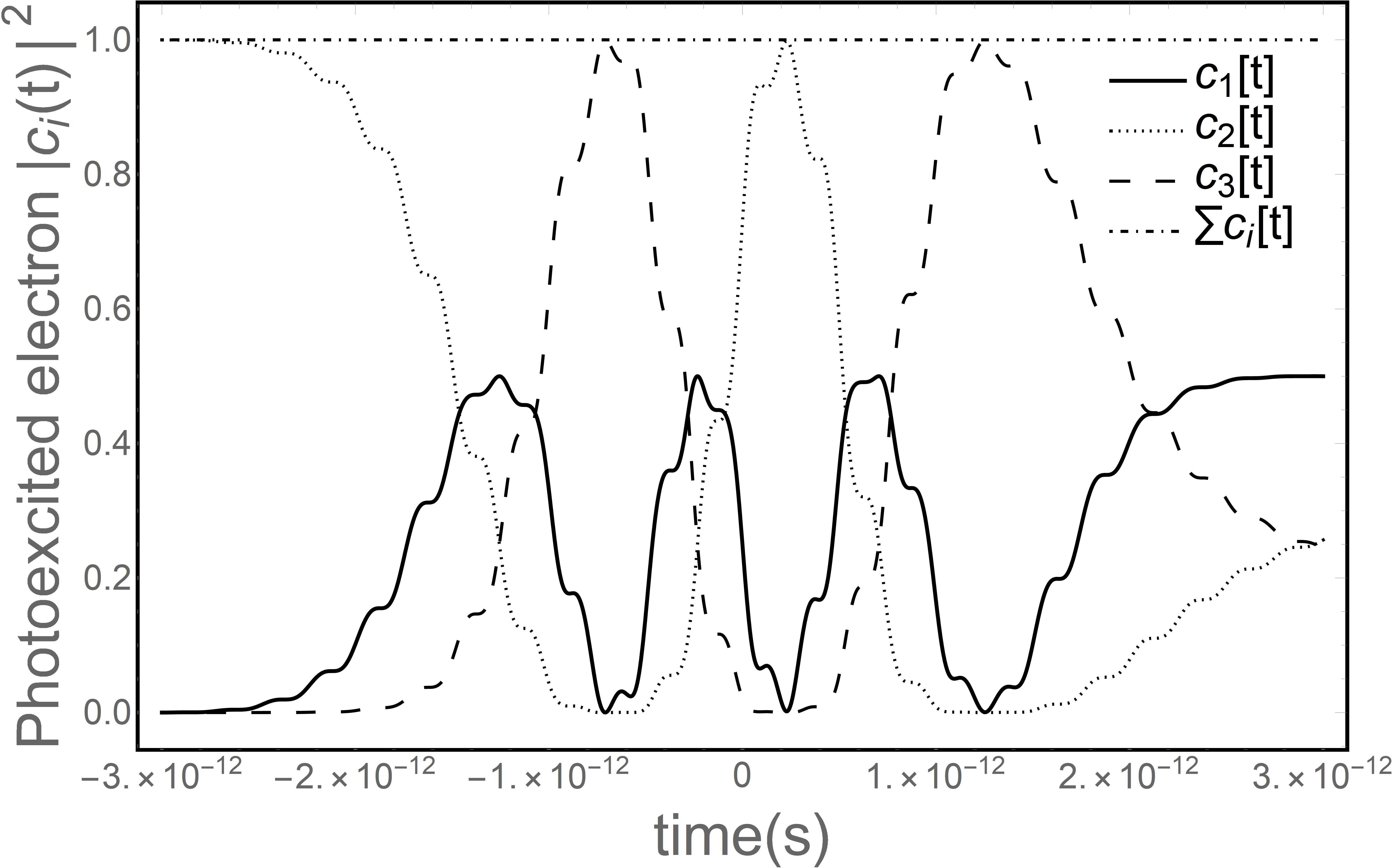
Figure 2: Electron dynamics at a resonant state $k=\omega_{0}/v_{0}$ and $\phi_{p}=\pi/4$ with incident light field $f_{0}=2\,\mathrm{THz}$, $\tau=1\,\mathrm{ps}$, and $I=1\,\mathrm{kW/cm^{2}}$

II.3 Induced Current Density in LCS Lattice

In order to simplify the notation used, at this point we transform the coefficients $\tilde{c}_{i}(t)$ into population inversions: $n_{12}(t)=|\tilde{c}_{1}(t)|^{2}-|\tilde{c}_{2}(t)|^{2}$, $n_{31}(t)=|\tilde{c}_{3}(t)|^{2}-|\tilde{c}_{1}(t)|^{2}$, $n_{32}(t)=|\tilde{c}_{3}(t)|^{2}-|\tilde{c}_{2}(t)|^{2}$, together with density matrix elements: $\rho_{ij}=\tilde{c}_{i}{\tilde{c}_{j}}^{\ast},(i,j=1,2,3)$. By introducing the continuity equation $\frac{\partial\rho}{\partial t}+\nabla\cdot{\bf j}=0$ with charge density $\rho=q|\Psi({\bf r},t)|^{2}$, we obtain expressions for the single-particle current density $j_{\nu}=e\Psi({\bf r},t)^{\dagger}\frac{\partial\textit{H}}{\hbar\partial k_{\nu}}\Psi({\bf r},t)$, where $\nu=x,y$ indicates the current density component, as follows:

$$j_{x}{(t)}=qv_{0}(1/2\pi)^{2}[\frac{n_{32}k_{x}}{k}+\frac{(\rho_{12}+\rho^{\ast}_{12})k_{y}-(\rho_{31}+\rho^{\ast}_{31})k_{y}}{\sqrt{2}k}],$$ (13a)

$$j_{y}{(t)}=qv_{0}(1/2\pi)^{2}[\frac{n_{32}k_{y}}{k}+\frac{(\rho_{31}+\rho^{\ast}_{31})k_{x}-(\rho_{12}+\rho^{\ast}_{12})k_{x}}{\sqrt{2}k}].$$ (13b)

Finally, the net (total) current density is obtained by integrating the single-particle current density over the momentum space:

$${\bf J}(t)=g_{s}\sum_{\bf k}{\bf j}(t),$$ (14)

where ${g_{s}}=2$ is the spin-degeneracy factor.

III RESULTS AND DISCUSSION

III.1 Single-Particle Harmonic Spectra with Rabi Oscillations

In Fig. 3, we plot the single-particle current spectra excited by a Gaussian (Fig. 3(a)) or square (Fig. 3(b)) pulse for resonant excitation at $k=\omega_{0}/\nu_{0}$ and $\phi_{k}=\pi/4$ with pump irradiance $I=500\,\mathrm{W/cm^{2}}$. The resultant single-particle current spectra are plotted in Figs. 3(c) and 3(d) respectively. These spectra exhibit energy at both even and odd harmonics. Further, the bandwidth over which significant energy content exists is quite large, ranging over at least the lowest five harmonics of the 2 THz fundamental excitation frequency. The detailed pulse shape is shown to impact the spectrum in a manner that is to be expected. The square pulse gives rise to sharper peaks in the spectrum than does the Gaussian pulse.

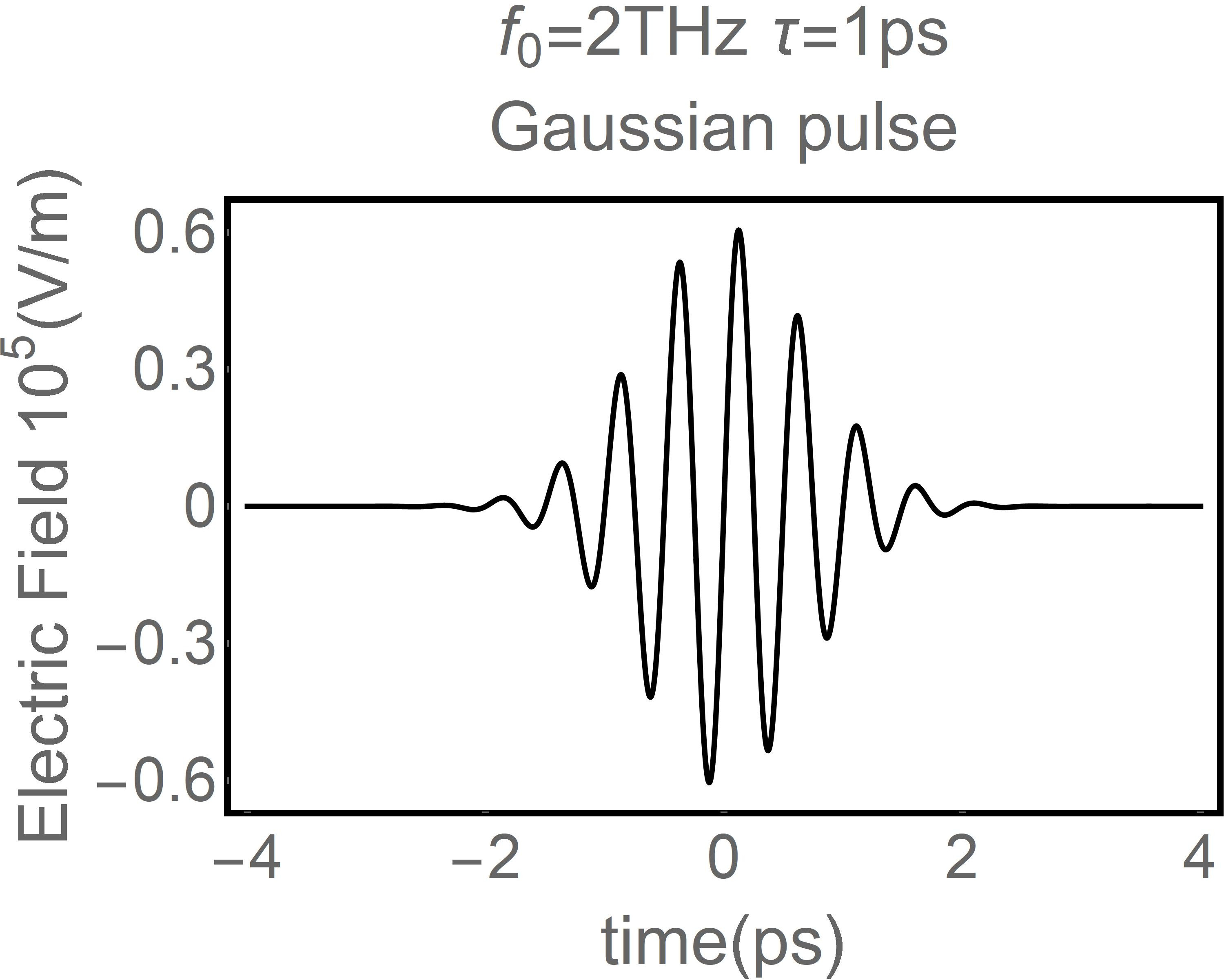
(a)

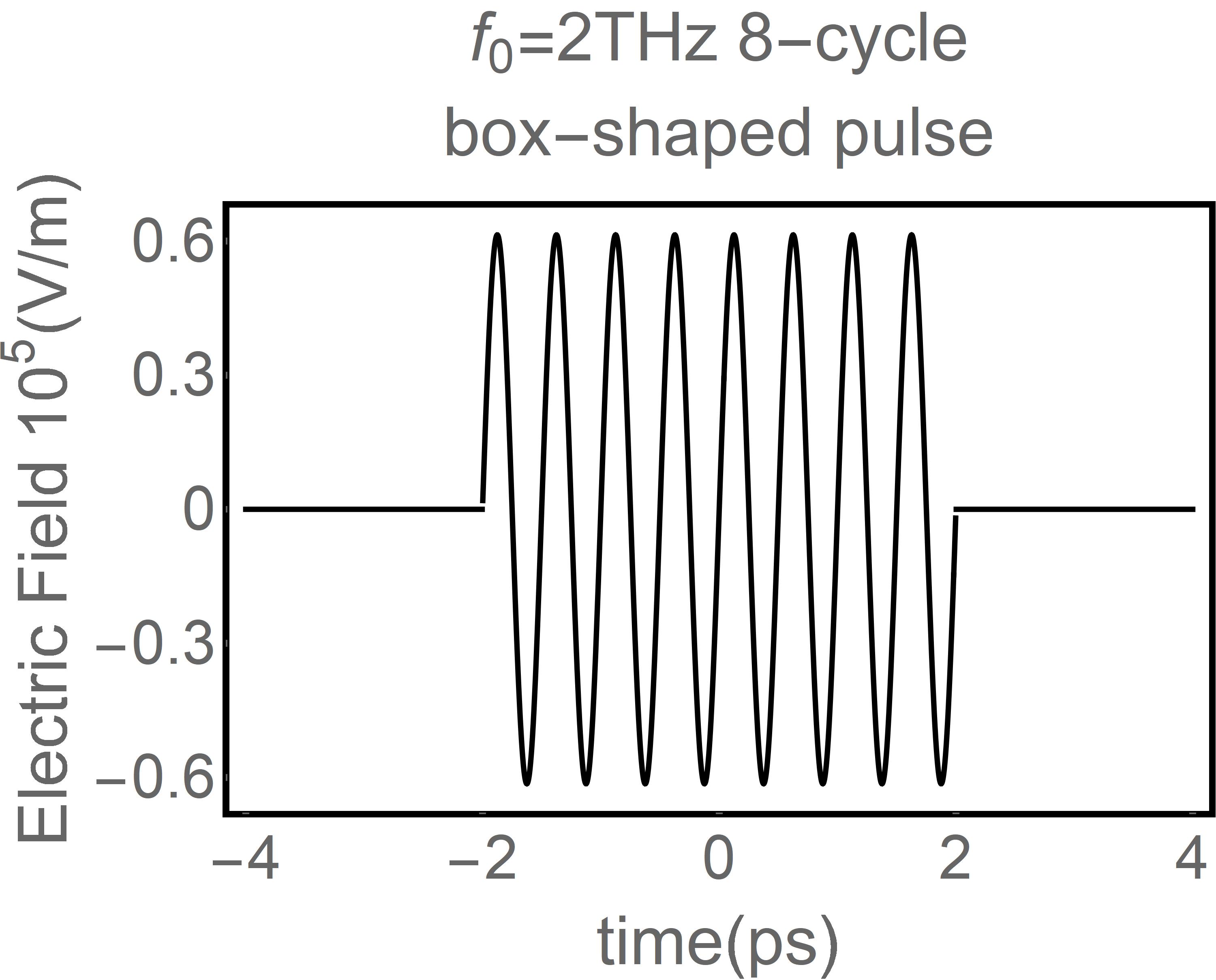
(b)

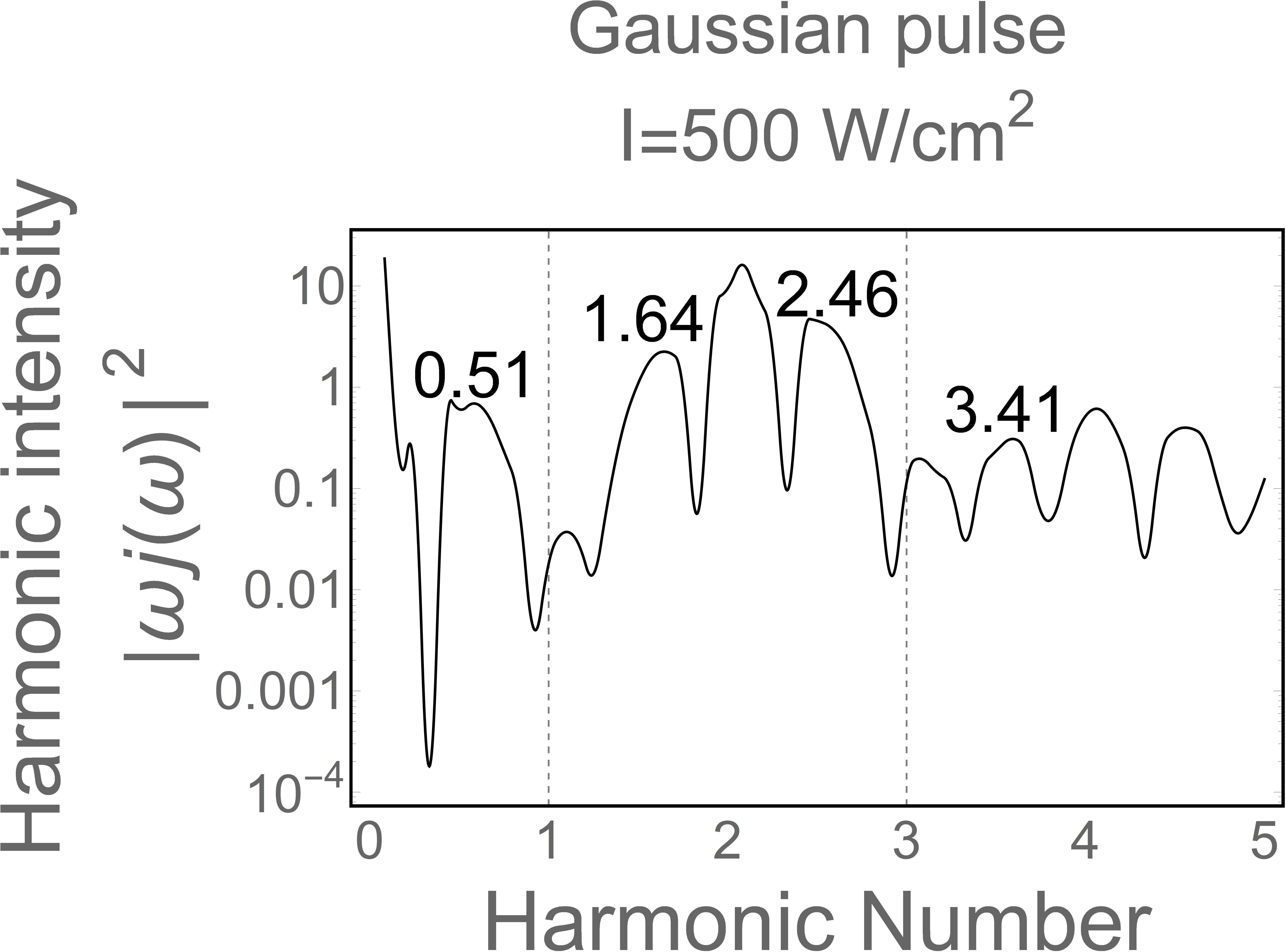
(c)

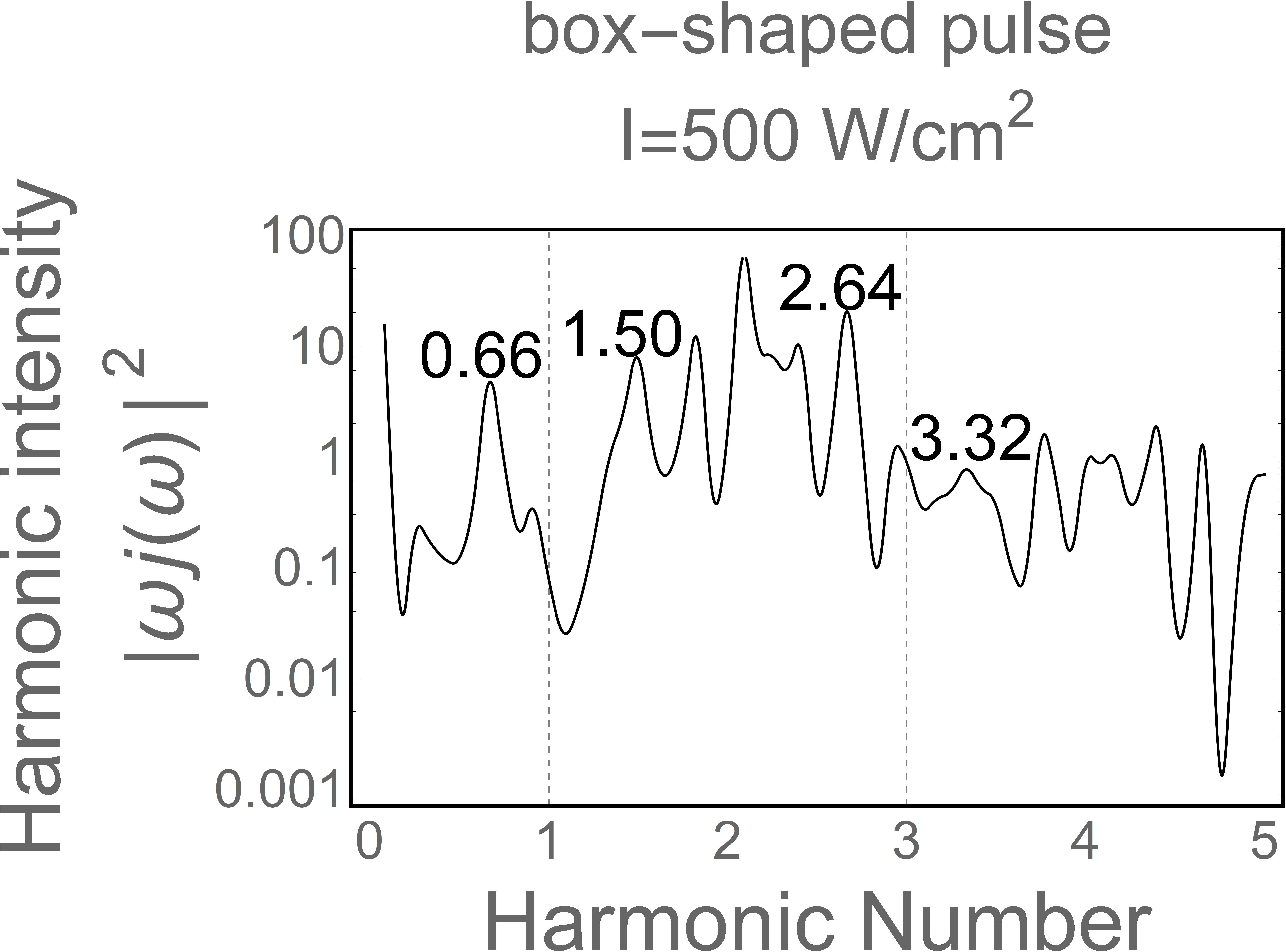
(d)

Figure 3: Illustration of the contribution from Rabi oscillations to the single-particle current spectra at $k=\omega_{0}/v_{0}$ with $\phi_{p}=\pi/4$ in the LCS lattice. A Gaussian pulse (a) with peak irradiance (c) $I=500W/cm^{2}$. A box-shaped pulse (b) with peak irradiance (d) $I=500\,\mathrm{W/cm^{2}}$.

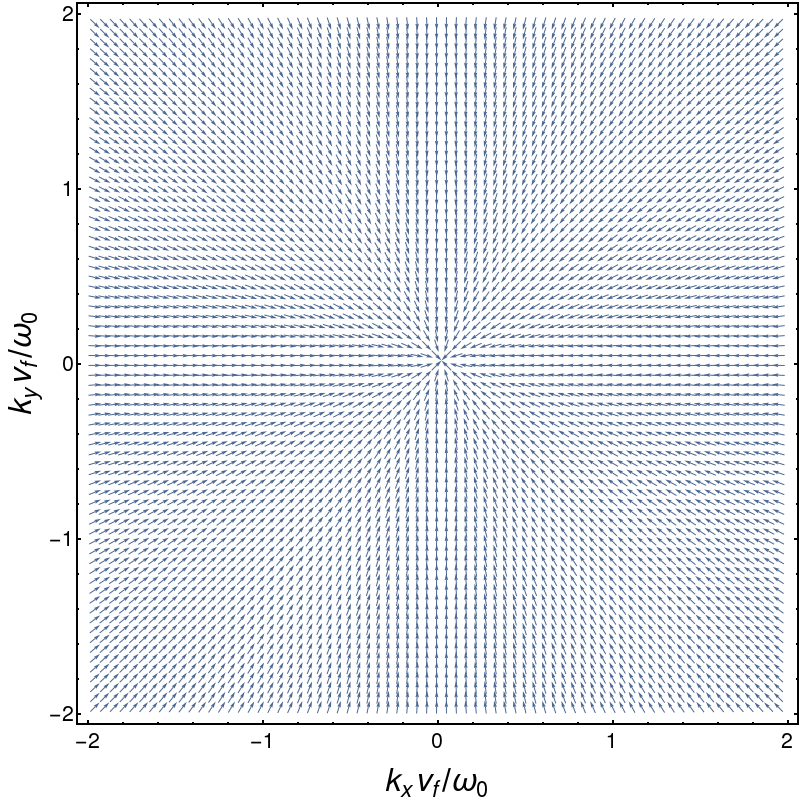
(a)

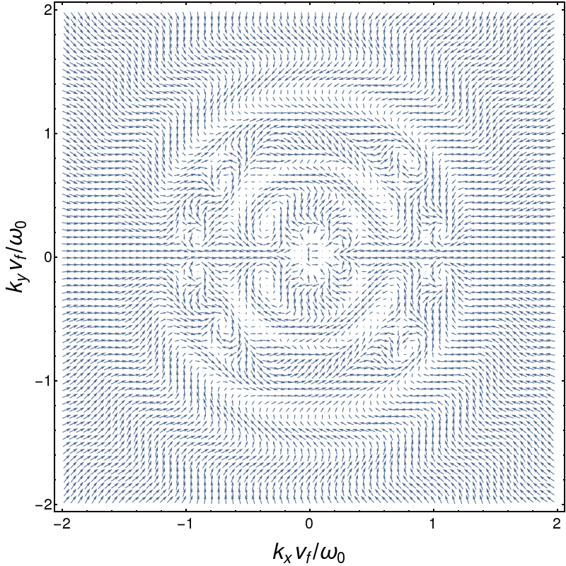
(b)

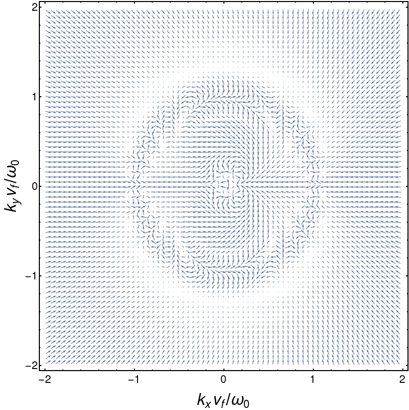
(c)

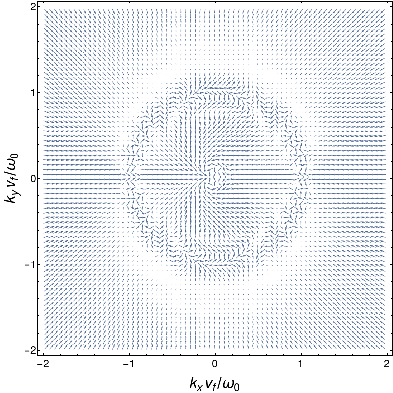
(d)

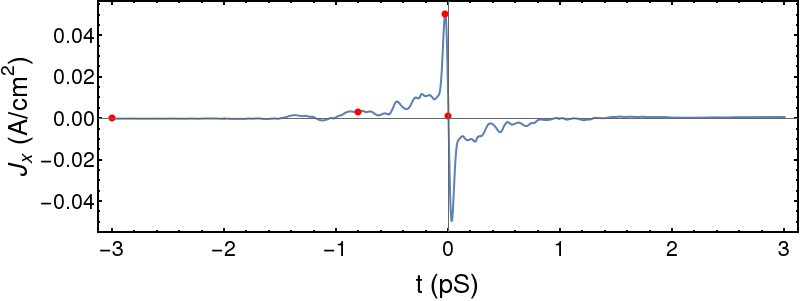
(e)

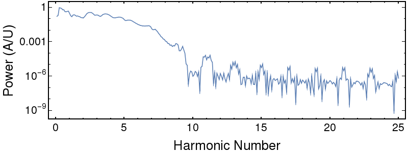
(f)

Figure 4: Current density for a peak pump irradiance of $I=10\,\mathrm{kW/cm^{2}}$. Plots a) through d) illustrate the magnitude and direction of the single-particle current density $\mathbf{j}$ at increasing time samples throughout the pump pulse. Plot e) shows the total current density $\mathbf{J}$ with the red dots indicating the temporal position of the single particle current density frames a)-d). Finally, plot f) shows the spectral power density of the total current density $\mathbf{J}$.

III.2 Total Current Spectral Content

Following Eq. 14, we obtain the total current by integrating numerically over $\mathbf{k}$. We have performed this calculation for pump irradiances ranging from $I=100\,\mathrm{W/cm^{2}}$ to $I=10\,\mathrm{kW/cm^{2}}$. In what follows, we characterize the spectral content of the total current over this complete pump range, however in the interest of conserving space, we plot the results only for the $I=10\,\mathrm{kW/cm^{2}}$ case in Fig. 4.

In Figs. 4(a)-4(d), we illustrate the magnitude and direction of the single-particle current density over a range of times relative to the pump pulse. Fig. 4(a) illustrates the thermal equilibrium current distribution prior to the arrival of the pump pulse. Figs. 4(b), 4(c), and 4(d) show the single-particle current density for times $800\,\mathrm{fs}$, $6\,\mathrm{fs}$, and $0\,\mathrm{fs}$ prior to the peak irradiance of the pump pulse respectively. These arrival times are noted as red dots on Fig. 4(e), which plots the temporal evolution of the total current density $\mathbf{J}$. We note that in our model, the total current density does not decay exactly to zero as the current dynamics disappear due to the passing pump pulse. Such a result is a consequence the fact that our model does not include a relaxation term. The absence of a relaxation term, coupled with the fact that the area of the $I=10\,\mathrm{kW/cm^{2}}$ pulse does not return the system exactly to its initial condition, results in a persistent offset in the plot of the temporal current density. Such an offset does not materially affect our conclusions.

Finally, in Fig. 4(f), we plot the spectrum of the total current density $\mathbf{J}$. The spectrum exhibits a continuum that persists up through the ninth harmonic. This continuum rolls off by two orders of magnitude at the high-frequency cutoff. At higher frequencies, the energy is localized around the odd harmonics as would be expected from a perturbation analysis of the problem due to the symmetry inherent in the LCS lattice. Each of the odd harmonics exhibits a bifurcation into a higher and lower frequency lobe surrounding the odd harmonic. This large spectral continuum may be understood by considering the evolution equations, Eqs. 10, 11, and 12. In this set of equations, the Rabi frequencies are proportional to $E_{x}(t)\sin\theta_{k}/k$. As a result, the frequency content of the total current ranges from a component with infinite frequency at $k=0$ to components with frequency asymptotically approaching 0 as $k\rightarrow\infty$. These components are weighted proportionally to $2\pi k$ due to the increasing density of states as $k$ increases.

Examining the resultant spectral content of the total current density for lower peak pump irradiances, we observe the following: for a peak pump irradiance of $1\,\mathrm{kW/cm^{2}}$, the continuum spectrum is down by two orders of magnitude relative to the low-frequency component of the total current density. Harmonics 1 (fundamental) and 3 bifurcate, whereas harmonics 5-11 are visible but do not bifurcate. For a peak pump irradiance of $100\,\mathrm{W/cm^{2}}$, the continuum is below the low frequency components by approximately the same two orders of magnitude, however only the fundamental frequency component bifurcates. Frequency components at harmonics 3-9 exist, but do not bifurcate at this irradiance.

Finally, we note that due to the mirror symmetry of the single-particle current density in the direction normal to the applied pump polarization, the total current in the direction normal to the polarization is zero.

IV Conclusion

In conclusion, we have analyzed the three-level LCS lattice and obtained closed-form expressions for the carrier dynamics in this system under the influence of a picosecond THz pump pulse polarized in the plane of the lattice. The total current density $\mathrm{J}$ arising in this system exhibits a spectral content that evolves toward a continuum at relatively moderate pump irradiances. We provide a detailed analysis of that continuum for a pump irradiance of $10\,\mathrm{kW/cm^{2}}$.