Successor Features Combine Elements of Model-Free and Model-based Reinforcement Learning

\nameLucas Lehnert \emaillucas_lehnert@brown.edu
\addrComputer Science Department
Carney Institute for Brain Science
Brown University
Providence, RI 02912, USA \AND\nameMichael L. Littman \emailmichael_littman@brown.edu
\addrComputer Science Department
Brown University
Providence, RI 02912, USA
Abstract

A key question in reinforcement learning is how an intelligent agent can generalize knowledge across different inputs. By generalizing across different inputs, information learned for one input can be immediately reused for improving predictions for another input. Reusing information allows an agent to compute an optimal decision-making strategy using less data. State representation is a key element of the generalization process, compressing a high-dimensional input space into a low-dimensional latent state space. This article analyzes properties of different latent state spaces, leading to new connections between model-based and model-free reinforcement learning. Successor features, which predict frequencies of future observations, form a link between model-based and model-free learning: Learning to predict future expected reward outcomes, a key characteristic of model-based agents, is equivalent to learning successor features. Learning successor features is a form of temporal difference learning and is equivalent to learning to predict a single policy’s utility, which is a characteristic of model-free agents. Drawing on the connection between model-based reinforcement learning and successor features, we demonstrate that representations that are predictive of future reward outcomes generalize across variations in both transitions and rewards. This result extends previous work on successor features, which is constrained to fixed transitions and assumes re-learning of the transferred state representation.

Keywords: Successor Features, Model-Based Reinforcement Learning, State Representations, State Abstractions

1 Introduction

A central question in Reinforcement Learning (RL) (Sutton and Barto, 2018) is how to process high dimensional inputs and compute decision-making strategies that maximize rewards. For example, a self-driving car has to process all its sensor data to decide when to accelerate or brake to drive the car safely. If the sensor data is high dimensional, obtaining an optimal decision-making strategy may become computationally very difficult because an optimal decision has to be computed for every possible sensor input. This “curse of dimensionality” (Bellman, 1961) can be overcome by compressing high dimensional sensor data into a lower dimensional latent state space. In the self-driving car example, if the car is following another vehicle that is stopping, detecting brake lights is sufficient to make the decision to slow the self-driving car down. Other information such as the colour of the car in front can be ignored. In RL, these decisions are grounded through a reward function, which would give high reward if the self-driving car reaches its destination and low reward if an accident is caused. An intelligent agent can simplify a task by mapping high-dimensional inputs into a lower dimensional latent state space, leading to faster learning because information can be reused across different inputs. This article addresses the question how different principles of compressing inputs are related to one another and demonstrates how an agent can learn to simplify one task to accelerate learning on a different previously unseen task.

Previous work presents algorithms that reuse Successor Features (SFs) (Barreto et al., 2017a) to initialize learning across tasks with different reward specifications, leading to improvements in learning speed in challenging control tasks (Barreto et al., 2018; Zhang et al., 2017; Kulkarni et al., 2016). This article follows a different methodology: By analyzing which properties different latent state spaces are predictive of, different models of generalizations are compared leading to new connections between latent state spaces that support either model-free RL or model-based RL. Model-free RL memorizes and makes predictions for one particular decision-making strategy, while model-based RL aims at predicting future reward outcomes for any arbitrary decision-making strategy. Our analysis demonstrates how previous formulations of SFs learn latent state spaces that are predictive of the optimal decision-making strategy and are thus akin to model-free RL. This article introduces a new model, called the Linear Successor Feature Model (LSFM), and presents results demonstrating that LSFMs learn latent state spaces that support model-based RL.

Latent state spaces model equivalences between different inputs and are suitable for transfer across different tasks only if these equivalences are preserved. Because LSFMs construct latent state spaces that extract equivalences of a task’s transition dynamics and rewards, they afford transfer to tasks that preserve these equivalences but have otherwise different transitions, rewards, or optimal decision-making strategies. Ultimately, by compressing a high-dimensional state space, the representation learned by an LSFM can enable a model-based agent to learn a model of an MDP and an optimal policy significantly faster than agents that do not use a state abstraction or use a state abstraction of a different type. In contrast to SFs, which afford transfer across tasks with different rewards but assume fixed transition dynamics (Barreto et al., 2017a; Stachenfeld et al., 2017), LSFMs remove the assumption of a fixed transition function. While SFs are re-learned and adjusted to find the optimal policy of a previously unseen task (Lehnert et al., 2017), the presented experiments outline how LSFMs can preserve the latent state space across different tasks and construct an optimal policy by using less data than tabular RL algorithms that do not generalize across inputs.

To unpack the different connection points and contributions, we start by first presenting the two state representation types in Section 2 and provide a formal introduction of successor features in Section 3. Subsequently, Section 4 introduces LSFMs and presents the main theoretical contributions showing how LSFMs can be used for model-based RL. Then, Section 5 presents the link to model-free learning and presents a sequence of examples and simulation illustrating to what extent the representations learned with LSFMs generalize across tasks with different transitions, rewards, and optimal policies.

2 Predictive State Representations

An RL task is formalized as a Markov Decision Processes (MDP) M=𝒮,𝒜,p,r,γ𝑀𝒮𝒜𝑝𝑟𝛾M=\langle\mathcal{S},\mathcal{A},p,r,\gamma\rangle, where the state space 𝒮𝒮\mathcal{S} describes all possible sensor inputs, and the finite action space 𝒜𝒜\mathcal{A} describes the space of all possible decisions. The state space 𝒮𝒮\mathcal{S} is assumed to be an arbitrary set and can either be finite or uncountably infinite. All results presented in this article are stated for arbitrary state spaces 𝒮𝒮\mathcal{S} unless specified otherwise. How the state changes over time is determined by the transition function p𝑝p, which specifies a probability or density function of reaching a next state ssuperscript𝑠s^{\prime} if an action a𝑎a is selected at state s𝑠s. Transitions are Markovian and the probability or density of transitioning to a state ssuperscript𝑠s^{\prime} is specified by p(s|s,a)𝑝conditionalsuperscript𝑠𝑠𝑎p(s^{\prime}|s,a). The reward function r:𝒮×𝒜×𝒮[R,R]:𝑟𝒮𝒜𝒮𝑅𝑅r:\mathcal{S}\times\mathcal{A}\times\mathcal{S}\to[-R,R] specifies which reward is given for each transition and rewards are bounded in magnitude by a constant R𝑅R\in\mathbb{R}. Besides assuming a bounded reward function, both reward and transition functions are assumed to be arbitrary.

A policy π𝜋\pi describes an agent’s decision-making strategy and specifies a probability π(s,a)𝜋𝑠𝑎\pi(s,a) of selecting an action a𝒜𝑎𝒜a\in\mathcal{A} at state s𝒮𝑠𝒮s\in\mathcal{S}. A policy’s performance is described by the value function

Vπ(s)=𝔼p,π[t=1γtr(st,at,st+1)|s1=s],V^{\pi}(s)=\mathbb{E}_{p,\pi}\left[\sum_{t=1}^{\infty}\gamma^{t}r(s_{t},a_{t},s_{t+1})\middle|s_{1}=s\right], (1)

which predicts the expected discounted return generated by selecting actions according to π𝜋\pi when trajectories are started at the state s𝑠s. The expectation111The subscript of the expectation operator 𝔼𝔼\mathbb{E} denotes the probability distributions or densities over which the expectation is computed. in Equation (1) is computed over all infinite length trajectories that select actions according to π𝜋\pi and start at state s𝑠s. Similarly, the Q-value function is defined as

Qπ(s,a)=𝔼p,π[t=1γtr(st,at,st+1)|s1=s,a1=a].Q^{\pi}(s,a)=\mathbb{E}_{p,\pi}\left[\sum_{t=1}^{\infty}\gamma^{t}r(s_{t},a_{t},s_{t+1})\middle|s_{1}=s,a_{1}=a\right]. (2)

The expectation of the Q-value function in Equation (2) is computed over all infinite length trajectories that start at state s𝑠s with action a𝑎a and then follow the policy π𝜋\pi.

A latent state space 𝒮ϕsubscript𝒮italic-ϕ\mathcal{S}_{\phi} is constructed using a state representation function ϕ:𝒮𝒮ϕ:italic-ϕ𝒮subscript𝒮italic-ϕ\phi:\mathcal{S}\to\mathcal{S}_{\phi}. A state representation can be understood as a compression of the state space, because two different states s𝑠s and s~~𝑠\tilde{s} can be assigned to the same latent state ϕ(s)=ϕ(s~)italic-ϕ𝑠italic-ϕ~𝑠\phi(s)=\phi(\tilde{s}). In this case, the state representation ϕitalic-ϕ\phi aliases s𝑠s and s~~𝑠\tilde{s}.

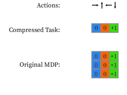
Figure 1(a) presents a grid world example where nine states are compressed into three different latent states and 𝒮ϕ={ϕ1,ϕ2,ϕ3}subscript𝒮italic-ϕsubscriptbold-italic-ϕ1subscriptbold-italic-ϕ2subscriptbold-italic-ϕ3\mathcal{S}_{\phi}=\{\boldsymbol{\phi}_{1},\boldsymbol{\phi}_{2},\boldsymbol{\phi}_{3}\}. In this example, the state representation partitions the state space along three different columns and constructs a smaller latent grid world of size 3×1313\times 1. If an intelligent agent uses this state representation for learning, the agent would only maintain information about which column it is in but not which row and effectively operate on this smaller latent 3×1313\times 1 grid world.

Refer to caption
(a) Column World Example
Refer to caption
(b) State Values Vπsuperscript𝑉𝜋V^{\pi}
Refer to caption
(c) Example Trajectory
Figure 1: State Representations Construct Lower Dimensional Latent State Spaces.  1(a): The column world example is a 3×3333\times 3 grid world where an agent can move up (action \uparrow), down (action \downarrow), left (action \leftarrow), or right (action \rightarrow) to adjacent grid cells and entering the right (green) column is rewarded. The number in each grid cell indicate the reward obtained by entering the respective cell. The state representation merges each column (colour) into a different latent state.  1(b): The lower panel presents a matrix plot of the state values Vπsuperscript𝑉𝜋V^{\pi} for a policy that selects actions uniformly at random. Grid cells of the same column have equal distance to the rewarding column and thus equal state values. Because this state representation only generalizes across states of the same column, the constructed latent state space can be used to predict the value function Vπsuperscript𝑉𝜋V^{\pi} as well. The top panel, which presents a matrix plot of state values for the three latent states, illustrates how the latent state space can be used for value predictions as well.  1(c): Using the latent state space, a latent 3×1313\times 1 MDP can be constructed. Both latent MDP and original MDP produce equal reward sequences for trajectories that follow the same action sequence and that start at corresponding states and latent states. The figure illustrates such an example trajectory that starts at (1,1) or latent state ϕisubscriptbold-italic-ϕ𝑖\boldsymbol{\phi}_{i} and then follows the action sequence ,,\rightarrow,\downarrow,\rightarrow. Selecting the action \downarrow is modeled as a self loop in the latent MDP. Both trajectories generate the same reward sequence of 0,0,10010,0,1. Intuitively, the compressed 3×1313\times 1 grid world simulates reward sequences in exactly the same way as the 3×3333\times 3 column world task.

2.1 Value-Predictive State Representations

A value-predictive state representation constructs a latent state space that retains enough information to support accurate value or Q-value predictions. Figure 1(b) shows that the value of states of the same column are equal. Suppose each latent state is represented as a one-hot bit vector222A one-hot bit vector 𝒆isubscript𝒆𝑖\boldsymbol{e}_{i} is a column vector of zeros but with the i𝑖ith entry set to one. Vectors are denoted with bold lower-case letters. Matrices are denoted with bold capitalized letters. in three dimensions and 𝒮ϕ={𝒆1,𝒆2,𝒆3}subscript𝒮italic-ϕsubscript𝒆1subscript𝒆2subscript𝒆3\mathcal{S}_{\phi}=\{\boldsymbol{e}_{1},\boldsymbol{e}_{2},\boldsymbol{e}_{3}\}. Because each grid cell is mapped to a one-hot bit vector, ϕ(s)=𝒆iitalic-ϕ𝑠subscript𝒆𝑖\phi(s)=\boldsymbol{e}_{i} for some index i𝑖i. Furthermore there exists a real valued vector 𝒗3𝒗superscript3\boldsymbol{v}\in\mathbb{R}^{3} such that

Vπ(s)=(ϕ(s))𝒗=𝒆i𝒗.superscript𝑉𝜋𝑠superscriptitalic-ϕ𝑠top𝒗superscriptsubscript𝒆𝑖top𝒗V^{\pi}(s)=(\phi(s))^{\top}\boldsymbol{v}=\boldsymbol{e}_{i}^{\top}\boldsymbol{v}. (3)

Because the state representation ϕitalic-ϕ\phi outputs one-hot bit vectors, each entry of the vector 𝒗𝒗\boldsymbol{v} contains the state value associated with one of the three columns. Similarly, the state representation ϕitalic-ϕ\phi can be used for Q-value predictions and for each action a𝑎a, Qπ(s,a)=𝒆i𝒒asuperscript𝑄𝜋𝑠𝑎superscriptsubscript𝒆𝑖topsubscript𝒒𝑎Q^{\pi}(s,a)=\boldsymbol{e}_{i}^{\top}\boldsymbol{q}_{a}, where 𝒒a3subscript𝒒𝑎superscript3\boldsymbol{q}_{a}\in\mathbb{R}^{3}. This article refers to such state representations that serve as basis functions (Sutton, 1996; Konidaris et al., 2011) for accurate value or Q-value predictions as value-predictive. Because value-predictive state representations are only required to be predictive of a particular policy π𝜋\pi, they implicitly depend on the policy π𝜋\pi.

2.2 Reward-Predictive State Representations

A reward-predictive state representation constructs a latent state space that retains enough information about the original state space to support accurate predictions of future expected reward outcomes. Figure 1(c) shows a trajectory that starts at grid cell (1,1) and follows an action sequence to produce a reward sequence of 0,0,10010,0,1. Because the state representation constructs a latent MDP that is a 3×1313\times 1 grid world, a trajectory starting at the latent grid cell ϕ1subscriptbold-italic-ϕ1\boldsymbol{\phi}_{1} and following the same action sequence results in a latent state sequence of ϕ1,ϕ2,ϕ2,ϕ3subscriptbold-italic-ϕ1subscriptbold-italic-ϕ2subscriptbold-italic-ϕ2subscriptbold-italic-ϕ3\boldsymbol{\phi}_{1},\boldsymbol{\phi}_{2},\boldsymbol{\phi}_{2},\boldsymbol{\phi}_{3}. If a positive reward is associated with entering the state ϕ3subscriptbold-italic-ϕ3\boldsymbol{\phi}_{3}, the latent grid world would also produce a reward sequence of 0,0,10010,0,1. For any start state and any arbitrary action sequence, both the latent grid world and the original grid world produce equal reward sequences. This property can be formalized using a family of functions {ft}tsubscriptsubscript𝑓𝑡𝑡\{f_{t}\}_{t\in\mathbb{N}} that predicts the expected reward outcome after executing an action sequence a1,,atsubscript𝑎1subscript𝑎𝑡a_{1},...,a_{t} starting at state s𝑠s:

ft:(s,a1,,at)𝔼p[rt|s,a1,,at].f_{t}:(s,a_{1},...,a_{t})\mapsto\mathbb{E}_{p}\left[r_{t}\middle|s,a_{1},...,a_{t}\right]. (4)

The expectation in Equation (4) is computed over all trajectories that start in state s𝑠s and follow the action sequence a1,,atsubscript𝑎1subscript𝑎𝑡a_{1},...,a_{t}. A state representation is reward-predictive if the function ftsubscript𝑓𝑡f_{t} can be re-parametrized in terms of the constructed latent state space and if there exists a family of functions {gt}tsubscriptsubscript𝑔𝑡𝑡\{g_{t}\}_{t\in\mathbb{N}} such that

t1,s,a1,,at,ft(s,a1,,at)=gt(ϕ(s),a1,,at).formulae-sequencefor-all𝑡1𝑠subscript𝑎1subscript𝑎𝑡subscript𝑓𝑡𝑠subscript𝑎1subscript𝑎𝑡subscript𝑔𝑡italic-ϕ𝑠subscript𝑎1subscript𝑎𝑡\forall t\geq 1,s,a_{1},...,a_{t},~{}f_{t}(s,a_{1},...,a_{t})=g_{t}(\phi(s),a_{1},...,a_{t}). (5)

Because reward-predictive state representations are designed to produce accurate predictions of future expected reward outcomes, they need to encode information about both the transition and reward functions. Unlike value-predictive state representations, reward-predictive state representations are independent of a particular policy.

2.3 Learning State Representations

Figure 1 presents an example where the same state representation is both value- and reward-predictive. In this article, we will present the distinctions and connection points between value-predictive and reward-predictive state representations. Further, we will discuss learning algorithms that search the space of all possible state representations to identify approximations of value- or reward-predictive state representations. The following results and examples demonstrate that value- and reward-predictive state representations can generalize across states very differently. Specifically, re-using a reward-predictive state representation ϕitalic-ϕ\phi across tasks can accelerate learning because a model-based agent only needs to construct the function gtsubscript𝑔𝑡g_{t} (which is defined on a small latent state space) for the new task instead of re-learning the function ftsubscript𝑓𝑡f_{t} from scratch. To ensure a fair comparison between different approximations, this article assumes that the dimensionality of the latent state space or the number of latent states is a fixed hyper-parameter.

3 Successor Features

Successor features (Barreto et al., 2017a) are a generalization of the Successor Representation (SR) (Dayan, 1993). The SR can be defined as follows: For finite state and action spaces, the transition probabilities while selecting actions according to a policy π𝜋\pi can be written as a stochastic transition matrix 𝑷πsuperscript𝑷𝜋\boldsymbol{P}^{\pi}. If the start state with index s𝑠s is represented as a one-hot bit vector 𝒆ssubscript𝒆𝑠\boldsymbol{e}_{s}, the probability distribution of reaching a state after one time step of executing policy π𝜋\pi can be written as a row vector 𝒆s𝑷πsuperscriptsubscript𝒆𝑠topsuperscript𝑷𝜋\boldsymbol{e}_{s}^{\top}\boldsymbol{P}^{\pi}. After t𝑡t time steps, the probability distribution over states can be written as a vector 𝒆s(𝑷π)tsuperscriptsubscript𝒆𝑠topsuperscriptsuperscript𝑷𝜋𝑡\boldsymbol{e}_{s}^{\top}(\boldsymbol{P}^{\pi})^{t}. Suppose the path across the state space has a random length that follows the Geometric distribution with parameter γ𝛾\gamma: At each time step, a biased coin is flipped and the path continues with probability γ𝛾\gamma. In this model, the probability vector of reaching different states in t𝑡t time steps is (1γ)γt1𝒆s(𝑷π)t1𝛾superscript𝛾𝑡1superscriptsubscript𝒆𝑠topsuperscriptsuperscript𝑷𝜋𝑡(1-\gamma)\gamma^{t-1}\boldsymbol{e}_{s}^{\top}(\boldsymbol{P}^{\pi})^{t}. Omitting the factor (1γ)1𝛾(1-\gamma), the SR recursively computes the marginal probabilities over all time steps:

𝚿π=t=1γt1(𝑷π)t1=𝑰+γ𝑷π𝚿π.superscript𝚿𝜋superscriptsubscript𝑡1superscript𝛾𝑡1superscriptsuperscript𝑷𝜋𝑡1𝑰𝛾superscript𝑷𝜋superscript𝚿𝜋\boldsymbol{\Psi}^{\pi}=\sum_{t=1}^{\infty}\gamma^{t-1}(\boldsymbol{P}^{\pi})^{t-1}=\boldsymbol{I}+\gamma\boldsymbol{P}^{\pi}\boldsymbol{\Psi}^{\pi}. (6)

Each entry (i,j)𝑖𝑗(i,j) of the matrix (1γ)𝚿π1𝛾superscript𝚿𝜋(1-\gamma)\boldsymbol{\Psi}^{\pi} contains the marginal probability across all possible durations of transitioning from state i𝑖i to state j𝑗j. Intuitively, the entry (i,j)𝑖𝑗(i,j) of the matrix 𝚿πsuperscript𝚿𝜋\boldsymbol{\Psi}^{\pi} can be understood as the frequency of encountering state j𝑗j when starting a path at state i𝑖i and following the policy π𝜋\pi. An action conditioned fSR describes the marginal probability across all possible durations of transitioning from state i𝑖i to state j𝑗j, but first a particular action a𝑎a is selected, and then a policy π𝜋\pi is followed:

𝚿aπ=def.t=1γt1𝑷a(𝑷π)t2=𝑰+γ𝑷a𝚿π,subscriptsuperscript𝚿𝜋𝑎def.superscriptsubscript𝑡1superscript𝛾𝑡1subscript𝑷𝑎superscriptsuperscript𝑷𝜋𝑡2𝑰𝛾subscript𝑷𝑎superscript𝚿𝜋\boldsymbol{\Psi}^{\pi}_{a}\overset{\text{def.}}{=}\sum_{t=1}^{\infty}\gamma^{t-1}\boldsymbol{P}_{a}(\boldsymbol{P}^{\pi})^{t-2}=\boldsymbol{I}+\gamma\boldsymbol{P}_{a}\boldsymbol{\Psi}^{\pi}, (7)

where 𝑷asubscript𝑷𝑎\boldsymbol{P}_{a} is the stochastic transition matrix describing all transition probabilities when action a𝑎a is selected. Because 𝑷asubscript𝑷𝑎\boldsymbol{P}_{a} is a stochastic matrix, it can be shown that 𝚿πsuperscript𝚿𝜋\boldsymbol{\Psi}^{\pi} is invertible and that there exists a one-to-one correspondence between each transition matrix and action-conditional SR matrix.333By Equation (6), 𝚿π=𝑰+γ𝑷π𝚿π𝑰=(𝑰γ𝑷π)𝚿π(𝚿π)1=𝑰γ𝑷πiffsuperscript𝚿𝜋𝑰𝛾superscript𝑷𝜋superscript𝚿𝜋𝑰𝑰𝛾superscript𝑷𝜋superscript𝚿𝜋iffsuperscriptsuperscript𝚿𝜋1𝑰𝛾superscript𝑷𝜋\boldsymbol{\Psi}^{\pi}=\boldsymbol{I}+\gamma\boldsymbol{P}^{\pi}\boldsymbol{\Psi}^{\pi}\iff\boldsymbol{I}=(\boldsymbol{I}-\gamma\boldsymbol{P}^{\pi})\boldsymbol{\Psi}^{\pi}\iff(\boldsymbol{\Psi}^{\pi})^{-1}=\boldsymbol{I}-\gamma\boldsymbol{P}^{\pi}. Equation (7) outlines how to construct 𝚿aπsubscriptsuperscript𝚿𝜋𝑎\boldsymbol{\Psi}^{\pi}_{a} from 𝑷asubscript𝑷𝑎\boldsymbol{P}_{a} for all actions. The reverse direction follows from 𝚿aπ=𝑰+γ𝑷a𝚿π(𝚿aπ𝑰)(𝚿π)1/γ=𝑷aiffsubscriptsuperscript𝚿𝜋𝑎𝑰𝛾subscript𝑷𝑎superscript𝚿𝜋subscriptsuperscript𝚿𝜋𝑎𝑰superscriptsuperscript𝚿𝜋1𝛾subscript𝑷𝑎\boldsymbol{\Psi}^{\pi}_{a}=\boldsymbol{I}+\gamma\boldsymbol{P}_{a}\boldsymbol{\Psi}^{\pi}\iff(\boldsymbol{\Psi}^{\pi}_{a}-\boldsymbol{I})(\boldsymbol{\Psi}^{\pi})^{-1}/\gamma=\boldsymbol{P}_{a}.

SFs combine this idea with arbitrary state representations. Given a state representation ϕitalic-ϕ\phi, the SF is a column vector defined for each state and action pair (Kulkarni et al., 2016; Zhang et al., 2017) and

𝝍π(s,a)=𝔼p,π[t=1γt1ϕst|s1=s,a1=a],\boldsymbol{\psi}^{\pi}(s,a)=\mathbb{E}_{p,\pi}\left[\sum_{t=1}^{\infty}\gamma^{t-1}\boldsymbol{\phi}_{s_{t}}\middle|s_{1}=s,a_{1}=a\right], (8)

where the expectation in Equation (8) is computed over all infinite length trajectories that start at state s𝑠s with action a𝑎a and then follow the policy π𝜋\pi. The output at state s𝑠s of the vector-valued state-representation function ϕitalic-ϕ\phi is denoted by ϕssubscriptbold-italic-ϕ𝑠\boldsymbol{\phi}_{s}. We will refer to this vector ϕssubscriptbold-italic-ϕ𝑠\boldsymbol{\phi}_{s} as either the latent vector or latent state. If following the policy π𝜋\pi leads to encountering a particular latent vector ϕssubscriptbold-italic-ϕsuperscript𝑠\boldsymbol{\phi}_{s^{\prime}} many times, then this latent vector will occur in the summation in Equation (8) many times.444The remainder of the article will list function arguments in the subscript of a symbol and ϕssubscriptbold-italic-ϕ𝑠\boldsymbol{\phi}_{s} always denotes the output of ϕitalic-ϕ\phi at state s𝑠s. Depending on the state representation ϕitalic-ϕ\phi, the vector 𝝍π(s,a)superscript𝝍𝜋𝑠𝑎\boldsymbol{\psi}^{\pi}(s,a) will be more similar to the latent vector ϕssubscriptbold-italic-ϕsuperscript𝑠\boldsymbol{\phi}_{s^{\prime}} and 𝝍π(s,a)superscript𝝍𝜋𝑠𝑎\boldsymbol{\psi}^{\pi}(s,a) will be more dis-similar to a latent vector ϕs~subscriptbold-italic-ϕ~𝑠\boldsymbol{\phi}_{\tilde{s}} if s~~𝑠\tilde{s} is a state that cannot be reached from the state s𝑠s. A SF vector 𝝍πsuperscript𝝍𝜋\boldsymbol{\psi}^{\pi} can be understood as a statistic measuring how frequently different latent states vectors are encountered.

The following two sections draw connections between SFs, reward-predictive, and value-predictive state representations and outline under what assumptions learning SFs is equivalent to learning reward- or value-predictive state representations.

4 Connections to Reward-Predictive Representations

A reward-predictive state representation constructs a latent state space that is rich enough to produce predictions of future expected reward outcomes for any arbitrary actions sequence. For accurate predictions, the empirical transition probabilities between latent states have to mimic transitions in the original task. Figure 2 presents a reward-prediction example where only one action is available to the agent. In this task, the goal is to predict that a positive reward is obtained in three time steps if the agent starts at state s1subscript𝑠1s_{1}. This example compares two different state representations, the representation ϕitalic-ϕ\phi, which does not compress the state space, and ϕ~~italic-ϕ\tilde{\phi}, which merges the first two states into one latent state. These two state representations lead to different empirical latent transition probabilities. While the first representation preserves the deterministic transitions of the task, the second representation does not. If states s1subscript𝑠1s_{1} and s2subscript𝑠2s_{2} are mapped to the same latent state ϕ~1subscript~bold-italic-ϕ1\tilde{\boldsymbol{\phi}}_{1}, then a transition from state s1subscript𝑠1s_{1} to s2subscript𝑠2s_{2} appears as a self-loop from latent state ϕ~1subscript~bold-italic-ϕ1\tilde{\boldsymbol{\phi}}_{1} to itself and a transition from s2subscript𝑠2s_{2} to s3subscript𝑠3s_{3} appears as a transition from ϕ~1subscript~bold-italic-ϕ1\tilde{\boldsymbol{\phi}}_{1} to ϕ~2subscript~bold-italic-ϕ2\tilde{\boldsymbol{\phi}}_{2}. Because the state representation ϕitalic-ϕ\phi constructs a latent state space with empirical latent transition probabilities that match the transition probabilities of the original task, this state representation is reward predictive.

from to ϕ1subscriptbold-italic-ϕ1\boldsymbol{\phi}_{1} ϕ2subscriptbold-italic-ϕ2\boldsymbol{\phi}_{2} ϕ3subscriptbold-italic-ϕ3\boldsymbol{\phi}_{3}
ϕ1subscriptbold-italic-ϕ1\boldsymbol{\phi}_{1} 0 1 0
ϕ2subscriptbold-italic-ϕ2\boldsymbol{\phi}_{2} 0 0 1
ϕ3subscriptbold-italic-ϕ3\boldsymbol{\phi}_{3} 0 0 1
s1subscript𝑠1s_{1}s2subscript𝑠2s_{2}s3subscript𝑠3s_{3}r=0𝑟0r=0r=0𝑟0r=0r=1𝑟1r=1ϕitalic-ϕ\phiϕ1subscriptbold-italic-ϕ1\boldsymbol{\phi}_{1}ϕ2subscriptbold-italic-ϕ2\boldsymbol{\phi}_{2}ϕ3subscriptbold-italic-ϕ3\boldsymbol{\phi}_{3}ϕ~~italic-ϕ\tilde{\phi}ϕ~1subscript~bold-italic-ϕ1\tilde{\boldsymbol{\phi}}_{1}ϕ~1subscript~bold-italic-ϕ1\tilde{\boldsymbol{\phi}}_{1}ϕ~2subscript~bold-italic-ϕ2\tilde{\boldsymbol{\phi}}_{2}
from to ϕ~1subscript~bold-italic-ϕ1\tilde{\boldsymbol{\phi}}_{1} ϕ~2subscript~bold-italic-ϕ2\tilde{\boldsymbol{\phi}}_{2}
ϕ~1subscript~bold-italic-ϕ1\tilde{\boldsymbol{\phi}}_{1} 0.5 0.5
ϕ~2subscript~bold-italic-ϕ2\tilde{\boldsymbol{\phi}}_{2} 0 1
Empirical LatentTransition Distribution with ϕitalic-ϕ\phi.Three-State MDP.Empirical LatentTransition Distribution with ϕ~~italic-ϕ\tilde{\phi}.
Figure 2: Three-State MDP Example. The centre schematic shows a single action three-state MDP with deterministic transitions (black arrows). Only the self-looping transition at state s3subscript𝑠3s_{3} is rewarded. The two state representations ϕitalic-ϕ\phi and ϕ~~italic-ϕ\tilde{\phi} map the three states to different feature vectors, resulting in different empirical feature-transition probabilities. These probabilities are computed from observed trajectories that start at state s1subscript𝑠1s_{1}.
Pr{s𝑎ϕ3}Pr𝑠𝑎subscriptbold-italic-ϕ3\text{Pr}\{s\overset{a}{\rightarrow}\boldsymbol{\phi}_{3}\}Pr{ϕ1𝑎ϕ3|ω}Prconditional-setsubscriptbold-italic-ϕ1𝑎subscriptbold-italic-ϕ3𝜔\text{Pr}\{\boldsymbol{\phi}_{1}\overset{a}{\rightarrow}\boldsymbol{\phi}_{3}|\omega\}𝒮𝒮\mathcal{S}ProbabilityDensityFeatureSpaces𝑠sϕ1subscriptbold-italic-ϕ1\boldsymbol{\phi}_{1}ϕ2subscriptbold-italic-ϕ2\boldsymbol{\phi}_{2}ϕ3subscriptbold-italic-ϕ3\boldsymbol{\phi}_{3}ϕ4subscriptbold-italic-ϕ4\boldsymbol{\phi}_{4}p(s,a,)𝑝𝑠𝑎p(s,a,\cdot)ω()𝜔\omega(\cdot) Pr{s𝑎ϕ3}Pr𝑠𝑎subscriptbold-italic-ϕ3\text{Pr}\{s\overset{a}{\rightarrow}\boldsymbol{\phi}_{3}\}: The probability of transitioning from s𝑠s to any state mapped to ϕ3subscriptbold-italic-ϕ3\boldsymbol{\phi}_{3} by selecting action a𝑎a. Pr{ϕ1𝑎ϕ3|ω}Prconditional-setsubscriptbold-italic-ϕ1𝑎subscriptbold-italic-ϕ3𝜔\text{Pr}\{\boldsymbol{\phi}_{1}\overset{a}{\rightarrow}\boldsymbol{\phi}_{3}|\omega\}: Empirical probability of transitioning from latent state ϕ1subscriptbold-italic-ϕ1\boldsymbol{\phi}_{1} to latent state ϕ3subscriptbold-italic-ϕ3\boldsymbol{\phi}_{3} by selecting action a𝑎a.
Figure 3: Empirical Latent Transition Probabilities Depend on State-Visitation Frequencies. This example illustrates how empirical latent transition probabilities depend on state-visitation frequencies. In this example, the state space 𝒮𝒮\mathcal{S} is a bounded interval in \mathbb{R} that is clustered into one of four latent states: ϕ1,ϕ2,ϕ3subscriptbold-italic-ϕ1subscriptbold-italic-ϕ2subscriptbold-italic-ϕ3\boldsymbol{\phi}_{1},\boldsymbol{\phi}_{2},\boldsymbol{\phi}_{3}, or ϕ4subscriptbold-italic-ϕ4\boldsymbol{\phi}_{4}. State-visitation frequencies are modeled for each partition independently using the density function ω𝜔\omega. The schematic plots the density function p𝑝p over states of selecting action a𝑎a at state s𝑠s (blue area) and the density function ω𝜔\omega over the state partition ϕ1subscriptbold-italic-ϕ1\boldsymbol{\phi}_{1} (orange area). The probability Pr{s𝑎ϕ3}Pr𝑠𝑎subscriptbold-italic-ϕ3\text{Pr}\{s\overset{a}{\rightarrow}\boldsymbol{\phi}_{3}\} of transitioning into the partition ϕ3subscriptbold-italic-ϕ3\boldsymbol{\phi}_{3} is the blue shaded area. The probability Pr{ϕ1𝑎ϕ3|ω}Prconditional-setsubscriptbold-italic-ϕ1𝑎subscriptbold-italic-ϕ3𝜔\text{Pr}\{\boldsymbol{\phi}_{1}\overset{a}{\rightarrow}\boldsymbol{\phi}_{3}|\omega\} of a transition from ϕ1subscriptbold-italic-ϕ1\boldsymbol{\phi}_{1} to ϕ3subscriptbold-italic-ϕ3\boldsymbol{\phi}_{3} occurring is the marginal of Pr{s𝑎ϕ3}Pr𝑠𝑎subscriptbold-italic-ϕ3\text{Pr}\{s\overset{a}{\rightarrow}\boldsymbol{\phi}_{3}\} over all states s𝑠s mapping to ϕ1subscriptbold-italic-ϕ1\boldsymbol{\phi}_{1}, weighted by ω𝜔\omega.

A reward-predictive state representation can be used in conjunction with a Linear Action Model (Sutton et al., 2008; Yao and Szepesvári, 2012) to compute expected future reward outcomes.

Definition 1 (Linear Action Model (LAM)).

Given an MDP and a state representation ϕ:𝒮n:italic-ϕ𝒮superscript𝑛\phi:\mathcal{S}\to\mathbb{R}^{n}, a LAM consists of a set of matrices and vectors {𝐌a,𝐰a}a𝒜subscriptsubscript𝐌𝑎subscript𝐰𝑎𝑎𝒜\{\boldsymbol{M}_{a},\boldsymbol{w}_{a}\}_{a\in\mathcal{A}}, where 𝐌asubscript𝐌𝑎\boldsymbol{M}_{a} is of size n×n𝑛𝑛n\times n and the column vector 𝐰asubscript𝐰𝑎\boldsymbol{w}_{a} is of dimension n𝑛n.

Given a fixed state representation, the transition matrices of a LAM {𝑴a}a𝒜subscriptsubscript𝑴𝑎𝑎𝒜\{\boldsymbol{M}_{a}\}_{a\in\mathcal{A}} model the empirical latent transition probabilities and the vectors {𝒘a}a𝒜subscriptsubscript𝒘𝑎𝑎𝒜\{\boldsymbol{w}_{a}\}_{a\in\mathcal{A}} model a linear map from latent states to expected one-step reward outcomes. The expected reward outcome after following the action sequence a1,,atsubscript𝑎1subscript𝑎𝑡a_{1},...,a_{t} starting at state s𝑠s can then be approximated with

𝔼p[rt|s,a1,,at]ϕs𝑴a1𝑴at1𝒘at.\mathbb{E}_{p}\left[r_{t}\middle|s,a_{1},...,a_{t}\right]\approx\boldsymbol{\phi}_{s}^{\top}\boldsymbol{M}_{a_{1}}\cdots\boldsymbol{M}_{a_{t-1}}\boldsymbol{w}_{a_{t}}. (9)

The following sections will address how a state representation ϕitalic-ϕ\phi and a LAM can be found to predict expected future reward outcomes as accurately as possible. Because this article’s goal is to establish different connections between learning successor features and model-based RL and to demonstrate that the learned reward-predictive state representations are suitable for transfer across variations in transitions and rewards, an extension of these model to non-linear latent transition and reward functions is left to future work.

To tie SFs to reward-predictive state representations, we first introduce a set of square real-valued matrices {𝑭a}a𝒜subscriptsubscript𝑭𝑎𝑎𝒜\{\boldsymbol{F}_{a}\}_{a\in\mathcal{A}} such that, for every state s𝑠s and action a𝑎a,

ϕs𝑭asuperscriptsubscriptbold-italic-ϕ𝑠topsubscript𝑭𝑎\displaystyle\boldsymbol{\phi}_{s}^{\top}\boldsymbol{F}_{a} 𝝍π(s,a)absentsuperscript𝝍𝜋𝑠𝑎\displaystyle\approx\boldsymbol{\psi}^{\pi}(s,a) (10)
=𝔼p,π[t=1γt1ϕst|s1=s,a1=a]\displaystyle=\mathbb{E}_{p,\pi}\left[\sum_{t=1}^{\infty}\gamma^{t-1}\boldsymbol{\phi}_{s_{t}}\middle|s_{1}=s,a_{1}=a\right] (11)

where the policy π𝜋\pi is defined on the latent state space. A Linear Successor Feature Model (LSFM) is then defined using the matrices {𝑭a}a𝒜subscriptsubscript𝑭𝑎𝑎𝒜\{\boldsymbol{F}_{a}\}_{a\in\mathcal{A}}:

Definition 2 (Linear Successor Feature Model (LSFM)).

Given an MDP, a policy π𝜋\pi, and a state representation ϕ:𝒮n:italic-ϕ𝒮superscript𝑛\phi:\mathcal{S}\to\mathbb{R}^{n}, an LSFM consists of a set of matrices and vectors {𝐅a,𝐰a}a𝒜subscriptsubscript𝐅𝑎subscript𝐰𝑎𝑎𝒜\{\boldsymbol{F}_{a},\boldsymbol{w}_{a}\}_{a\in\mathcal{A}}, where 𝐅asubscript𝐅𝑎\boldsymbol{F}_{a} is of size n×n𝑛𝑛n\times n and the column vector 𝐰asubscript𝐰𝑎\boldsymbol{w}_{a} is of dimension n𝑛n. The matrices {𝐅a}a𝒜subscriptsubscript𝐅𝑎𝑎𝒜\{\boldsymbol{F}_{a}\}_{a\in\mathcal{A}} are used to model a linear map from latent state features to SFs as described in Equation (10).

LSFMs require the state representation ϕitalic-ϕ\phi to (linearly) approximate the SF 𝝍π(s,a)superscript𝝍𝜋𝑠𝑎\boldsymbol{\psi}^{\pi}(s,a) using the matrices {𝑭a}a𝒜subscriptsubscript𝑭𝑎𝑎𝒜\{\boldsymbol{F}_{a}\}_{a\in\mathcal{A}} (Equation (10)). Previously presented SF frameworks (Barreto et al., 2017a, 2018) do not use the state representation ϕitalic-ϕ\phi to approximate SF vectors 𝝍πsuperscript𝝍𝜋\boldsymbol{\psi}^{\pi} as described in Equation (10) and construct the state-representation function ϕitalic-ϕ\phi differently, for example, by setting the output of ϕitalic-ϕ\phi to be one-step rewards (Barreto et al., 2017b). In contrast, LSFMs are used to learn the state-representation function ϕitalic-ϕ\phi that satisfies Equation (10). Because LSFMs distinctly incorporate this approximative property, SFs can be connected to model-based RL.

An intelligent agent that uses a state representation ϕitalic-ϕ\phi operates directly on the constructed latent state space and is constrained to only search the space of policies that are defined on its latent state space. These policies are called abstract policies.

Definition 3 (Abstract Policies).

An abstract policy πϕsubscript𝜋italic-ϕ\pi_{\phi} is a function mapping latent state and action pairs to probability values:

s𝒮,a𝒜,πϕ(ϕs,a)[0,1]andaπϕ(ϕs,a)=1.formulae-sequencefor-all𝑠𝒮formulae-sequence𝑎𝒜subscript𝜋italic-ϕsubscriptbold-italic-ϕ𝑠𝑎01andsubscript𝑎subscript𝜋italic-ϕsubscriptbold-italic-ϕ𝑠𝑎1\forall s\in\mathcal{S},a\in\mathcal{A},\pi_{\phi}(\boldsymbol{\phi}_{s},a)\in[0,1]~{}\text{and}~{}\sum_{a}\pi_{\phi}(\boldsymbol{\phi}_{s},a)=1.

For a fixed state representation ϕitalic-ϕ\phi, the set of all abstract policies is denoted with ΠϕsubscriptΠitalic-ϕ\Pi_{\phi}.

The following sections first tie learning LAMs to reward-predictive state representations. We then show that learning LSFMs is equivalent to learning LAMs tying LSFMs to reward-predictive state representations.

4.1 Encoding Bisimulation Relations

To ensure accurate predictions of future reward outcomes, the previous discussion suggests that the empirical latent transition probabilities have to match the transition probabilities in the original task. Figure 3 presents a schematic explaining these dependencies further. In this example, the state space is a bounded interval in \mathbb{R} that is mapped to four different latent states, ϕ1subscriptbold-italic-ϕ1\boldsymbol{\phi}_{1}, ϕ2subscriptbold-italic-ϕ2\boldsymbol{\phi}_{2}, ϕ3subscriptbold-italic-ϕ3\boldsymbol{\phi}_{3}, or ϕ4subscriptbold-italic-ϕ4\boldsymbol{\phi}_{4}. The probability of transitioning from the state s𝑠s to any state that is mapped to ϕ3subscriptbold-italic-ϕ3\boldsymbol{\phi}_{3} is denoted with Pr{s𝑎ϕ3}Pr𝑠𝑎subscriptbold-italic-ϕ3\text{Pr}\{s\overset{a}{\to}\boldsymbol{\phi}_{3}\}. This probability Pr{s𝑎ϕ3}Pr𝑠𝑎subscriptbold-italic-ϕ3\text{Pr}\{s\overset{a}{\to}\boldsymbol{\phi}_{3}\} is the marginal over all states ssuperscript𝑠s^{\prime} that are mapped to the latent state ϕ3subscriptbold-italic-ϕ3\boldsymbol{\phi}_{3}. Assume that ω𝜔\omega is a density function over all states that are mapped to the latent state ϕ1subscriptbold-italic-ϕ1\boldsymbol{\phi}_{1}. This density function could model the visitation frequencies of different states as an intelligent agent interacts with the MDP. The empirical probability of transitioning from latent state ϕ1subscriptbold-italic-ϕ1\boldsymbol{\phi}_{1} to ϕ3subscriptbold-italic-ϕ3\boldsymbol{\phi}_{3} is then the marginal over all states mapping to ϕ1subscriptbold-italic-ϕ1\boldsymbol{\phi}_{1} and

Pr{ϕ1𝑎ϕ3|ω}=s:ϕ(s)=ϕ1ω(s)Pr{s𝑎ϕ3}ds=𝔼ω[Pr{s𝑎ϕ3}|ϕ(s)=ϕ1].\text{Pr}\left\{\boldsymbol{\phi}_{1}\overset{a}{\to}\boldsymbol{\phi}_{3}\middle|\omega\right\}=\int_{s:\phi(s)=\boldsymbol{\phi}_{1}}\omega(s)\text{Pr}\{s\overset{a}{\to}\boldsymbol{\phi}_{3}\}ds=\mathbb{E}_{\omega}\left[\text{Pr}\{s\overset{a}{\to}\boldsymbol{\phi}_{3}\}\middle|\phi(s)=\boldsymbol{\phi}_{1}\right]. (12)

The expectation in Equation (12) is computed with respect to ω𝜔\omega over all states s𝑠s that map to the latent state ϕ1subscriptbold-italic-ϕ1\boldsymbol{\phi}_{1}. As Equation (12) outlines, the empirical transition probability Pr{ϕ1𝑎ϕ3|ω}Prconditional-setsubscriptbold-italic-ϕ1𝑎subscriptbold-italic-ϕ3𝜔\text{Pr}\{\boldsymbol{\phi}_{1}\overset{a}{\to}\boldsymbol{\phi}_{3}|\omega\} depends on the visitation frequencies ω𝜔\omega. The probability Pr{s𝑎ϕ3}Pr𝑠𝑎subscriptbold-italic-ϕ3\text{Pr}\{s\overset{a}{\to}\boldsymbol{\phi}_{3}\} of transitioning from a state s𝑠s into a partition only depends on the transition function p𝑝p itself.

Consider two different states s𝑠s and s~~𝑠\tilde{s} that map to the same latent state and ϕ(s)=ϕ(s~)italic-ϕ𝑠italic-ϕ~𝑠\phi(s)=\phi(\tilde{s}). If the state representation is constructed such that

a,ϕi,Pr{s𝑎ϕi}=Pr{s~𝑎ϕi}and𝔼p[r(s,a,s)|s,a]=𝔼p[r(s~,a,s)|s~,a],\forall a,\forall\boldsymbol{\phi}_{i},~{}\text{Pr}\{s\overset{a}{\to}\boldsymbol{\phi}_{i}\}=\text{Pr}\{\tilde{s}\overset{a}{\to}\boldsymbol{\phi}_{i}\}~{}\text{and}~{}\mathbb{E}_{p}\left[r(s,a,s^{\prime})\middle|s,a\right]=\mathbb{E}_{p}\left[r(\tilde{s},a,s^{\prime})\middle|\tilde{s},a\right], (13)

then the empirical latent state transition probabilities would become independent of ω𝜔\omega because the integrand in Equation (12) is constant and

Pr{ϕ1𝑎ϕ3|ω}=s:ϕ(s)=ϕ1ω(s)Pr{s𝑎ϕ3}constant𝑑s=Pr{s𝑎ϕ3}.Prconditional-setsubscriptbold-italic-ϕ1𝑎subscriptbold-italic-ϕ3𝜔subscript:𝑠italic-ϕ𝑠subscriptbold-italic-ϕ1𝜔𝑠subscriptPr𝑠𝑎subscriptbold-italic-ϕ3constantdifferential-d𝑠Pr𝑠𝑎subscriptbold-italic-ϕ3\text{Pr}\left\{\boldsymbol{\phi}_{1}\overset{a}{\to}\boldsymbol{\phi}_{3}\middle|\omega\right\}=\int_{s:\phi(s)=\boldsymbol{\phi}_{1}}\omega(s)\underbrace{\text{Pr}\{s\overset{a}{\to}\boldsymbol{\phi}_{3}\}}_{\text{constant}}ds=\text{Pr}\{s\overset{a}{\to}\boldsymbol{\phi}_{3}\}. (14)

Equation (14) follows directly from the transition condition in line (13), because the probability Pr{s𝑎ϕ3}Pr𝑠𝑎subscriptbold-italic-ϕ3\text{Pr}\{s\overset{a}{\rightarrow}\boldsymbol{\phi}_{3}\} is constant for all states s𝑠s that are mapped to the latent state vector ϕ1subscriptbold-italic-ϕ1\boldsymbol{\phi}_{1}. If the two identities in line (13) hold, then the resulting latent state space constructs latent transition probabilities that correspond to the transition probabilities in the original task. Equation (13) describes an informal definition of bisimulation (Givan et al., 2003). Definition 4 listed in Appendix A.1 presents a formal measure theoretic definition of bisimulation on arbitrary (measurable) state spaces. This definition is used to prove the theorems stated in this section. To prove that LAMs encode state representations that generalize only across bisimilar states, two assumptions are made.

Assumption 1.

The state space 𝒮𝒮\mathcal{S} of an MDP can be partitioned into at most n𝑛n different partitions of bisimilar states, where n𝑛n is a natural number.

Assumption 2.

A state representation ϕ:𝒮{𝐞1,,𝐞n}:italic-ϕ𝒮subscript𝐞1subscript𝐞𝑛\phi:\mathcal{S}\to\{\boldsymbol{e}_{1},...,\boldsymbol{e}_{n}\} is assumed to have a range that consists of all n𝑛n one-hot bit vectors. For each i𝑖i, there exists a state s𝑠s such that ϕ(s)=𝐞iitalic-ϕ𝑠subscript𝐞𝑖\phi(s)=\boldsymbol{e}_{i}.

Assumption 1 is not particularly restrictive in a learning context: If an agent has observed n𝑛n distinct states during training, then a state representation assigning each state to one of n𝑛n different one-hot bit vectors can always be constructed. While doing so may not be useful to generalize across different states, this argument suggests that Assumption 1 is not restrictive in practice. Assumption 2 is relaxed in the following sections.

If action a𝑎a is selected at state s𝑠s, the expected next feature vector is

𝔼p[ϕ(s)|s,a]=j=1nPr{s𝑎𝒆j}𝒆j=[,Pr{s𝑎𝒆j},].\mathbb{E}_{p}\left[\phi(s^{\prime})\middle|s,a\right]=\sum_{j=1}^{n}\text{Pr}\{s\overset{a}{\to}\boldsymbol{e}_{j}\}\boldsymbol{e}_{j}=\left[\cdots,\text{Pr}\{s\overset{a}{\to}\boldsymbol{e}_{j}\},\cdots\right]^{\top}. (15)

The expected value in Equation (15) is computed over all possible next states ssuperscript𝑠s^{\prime} that can be reached from state s𝑠s by selecting action a𝑎a. In Equation (15), the next state ssuperscript𝑠s^{\prime} is a random variable whose probability distribution or density function is described by the MDP’s transition function p𝑝p. By Assumption 2, each state is mapped to some one-hot bit vector 𝒆jsubscript𝒆𝑗\boldsymbol{e}_{j}. Because there are only n𝑛n different one-hot bit vectors of dimension n𝑛n, the summation in Equation (15) is finite. Each entry of the resulting vector in Equation (15) stores the probability Pr{s𝑎𝒆j}Pr𝑠𝑎subscript𝒆𝑗\text{Pr}\{s\overset{a}{\to}\boldsymbol{e}_{j}\} of observing the feature vector 𝒆jsubscript𝒆𝑗\boldsymbol{e}_{j} after selecting action a𝑎a at state s𝑠s.

Because the expected next feature vector 𝔼p[ϕ(s)|s,a]\mathbb{E}_{p}\left[\phi(s^{\prime})\middle|s,a\right] is a probability vector, the transition matrices {𝑴a}a𝒜subscriptsubscript𝑴𝑎𝑎𝒜\{\boldsymbol{M}_{a}\}_{a\in\mathcal{A}} of a LAM are stochastic: If ϕ(s)=𝒆iitalic-ϕ𝑠subscript𝒆𝑖\phi(s)=\boldsymbol{e}_{i} and 𝒆i𝑴a=𝔼p[𝒆j|s,a]\boldsymbol{e}_{i}^{\top}\boldsymbol{M}_{a}=\mathbb{E}_{p}\left[\boldsymbol{e}_{j}\middle|s,a\right], then the i𝑖ith row of the matrix 𝑴asubscript𝑴𝑎\boldsymbol{M}_{a} is equal to the probability vector shown in Equation (15). If 𝒆i𝒘a=𝔼p[r(s,a,s)|s,a]\boldsymbol{e}_{i}^{\top}\boldsymbol{w}_{a}=\mathbb{E}_{p}\left[r(s,a,s^{\prime})\middle|s,a\right], then the weight vectors of a LAM {𝒘a}a𝒜subscriptsubscript𝒘𝑎𝑎𝒜\{\boldsymbol{w}_{a}\}_{a\in\mathcal{A}} encode a reward table. These observations lead to the first theorem.555Appendix A.1 presents formal proofs for all presented theorems.

Theorem 1.

For an MDP 𝒮,𝒜,p,r,γ𝒮𝒜𝑝𝑟𝛾\langle\mathcal{S},\mathcal{A},p,r,\gamma\rangle, let ϕ:𝒮{𝐞1,,𝐞n}:italic-ϕ𝒮subscript𝐞1subscript𝐞𝑛\phi:\mathcal{S}\to\{\boldsymbol{e}_{1},...,\boldsymbol{e}_{n}\} be a state representation and {𝐌a,𝐰a}a𝒜subscriptsubscript𝐌𝑎subscript𝐰𝑎𝑎𝒜\{\boldsymbol{M}_{a},\boldsymbol{w}_{a}\}_{a\in\mathcal{A}} a LAM. Assume that 𝒮𝒮\mathcal{S} can be partitioned into at most n𝑛n partitions of bisimilar states. If the state representation ϕitalic-ϕ\phi satisfies

s𝒮,a𝒜,ϕs𝒘a=𝔼p[r(s,a,s)|s,a]and ϕs𝑴a=𝔼p[ϕs|s,a],\forall s\in\mathcal{S},\forall a\in\mathcal{A},~{}\boldsymbol{\phi}_{s}^{\top}\boldsymbol{w}_{a}=\mathbb{E}_{p}\left[r(s,a,s^{\prime})\middle|s,a\right]~{}\text{and }~{}\boldsymbol{\phi}_{s}^{\top}\boldsymbol{M}_{a}=\mathbb{E}_{p}\left[\boldsymbol{\phi}_{s^{\prime}}\middle|s,a\right], (16)

then ϕitalic-ϕ\phi generalizes across bisimilar states and any two states s𝑠s and s~~𝑠\tilde{s} are bisimilar if ϕs=ϕs~subscriptbold-ϕ𝑠subscriptbold-ϕ~𝑠\boldsymbol{\phi}_{s}=\boldsymbol{\phi}_{\tilde{s}}.

The proof of Theorem 1 uses the fact that the expected value of one-hot bit vectors encode exact probability values. A similar observation can be made about the SFs for a one-hot bit-vector state representation. In this case, the (1γ)1𝛾(1-\gamma) rescaled SF contains the marginal of reaching a state partition across time steps:

(1γ)𝔼p,π[t=1γt1𝒆t|s,a1]=[,t=1(1γ)γt1𝔼p,π[Pr{sa1at𝒆i}|s,a1],],(1-\gamma)\mathbb{E}_{p,\pi}\left[\sum_{t=1}^{\infty}\gamma^{t-1}\boldsymbol{e}_{t}\middle|s,a_{1}\right]=\left[...,\sum_{t=1}^{\infty}(1-\gamma)\gamma^{t-1}\mathbb{E}_{p,\pi}\left[\text{Pr}\left\{s\overset{a_{1}\cdots a_{t}}{\longrightarrow}\boldsymbol{e}_{i}\right\}\middle|s,a_{1}\right],...\right]^{\top}, (17)

where the expectation in Equation (17) is computed over infinite length trajectories starting at state s𝑠s with action a𝑎a. This observation leads to the following theorem stating that LSFMs can be used to identify a one-hot state representation that generalizes across bisimilar states.

Theorem 2.

For an MDP 𝒮,𝒜,p,r,γ𝒮𝒜𝑝𝑟𝛾\langle\mathcal{S},\mathcal{A},p,r,\gamma\rangle, let ϕ:𝒮{𝐞1,,𝐞n}:italic-ϕ𝒮subscript𝐞1subscript𝐞𝑛\phi:\mathcal{S}\to\{\boldsymbol{e}_{1},...,\boldsymbol{e}_{n}\} be a state representation and {𝐅a,𝐰a}a𝒜subscriptsubscript𝐅𝑎subscript𝐰𝑎𝑎𝒜\{\boldsymbol{F}_{a},\boldsymbol{w}_{a}\}_{a\in\mathcal{A}} an LSFM. If, for one policy πΠϕ𝜋subscriptΠitalic-ϕ\pi\in\Pi_{\phi}, the representation ϕitalic-ϕ\phi satisfies

s𝒮,a𝒜,ϕs𝒘a=𝔼p[r(s,a,s)|s,a]andϕs𝑭a=ϕs+γ𝔼p,π[ϕs𝑭a|s,a],\forall s\in\mathcal{S},\forall a\in\mathcal{A},~{}\boldsymbol{\phi}_{s}^{\top}\boldsymbol{w}_{a}=\mathbb{E}_{p}\left[r(s,a,s^{\prime})\middle|s,a\right]~{}\text{and}~{}\boldsymbol{\phi}_{s}^{\top}\boldsymbol{F}_{a}=\boldsymbol{\phi}_{s}^{\top}+\gamma\mathbb{E}_{p,\pi}\left[\boldsymbol{\phi}_{s^{\prime}}\boldsymbol{F}_{a^{\prime}}\middle|s,a\right], (18)

then ϕitalic-ϕ\phi generalizes across bisimilar states and any two states s𝑠s and s~~𝑠\tilde{s} are bisimilar if ϕs=ϕs~subscriptbold-ϕ𝑠subscriptbold-ϕ~𝑠\boldsymbol{\phi}_{s}=\boldsymbol{\phi}_{\tilde{s}}. If Equation (18) holds for one policy πΠϕ𝜋subscriptΠitalic-ϕ\pi\in\Pi_{\phi}, then Equation (18) also holds every other policy π~Πϕ~𝜋subscriptΠitalic-ϕ\tilde{\pi}\in\Pi_{\phi} as well.

Equation (18) describes a fixed-point equation similar to the Bellman fixed-point equation:

𝒆s𝑭asuperscriptsubscript𝒆𝑠topsubscript𝑭𝑎\displaystyle\boldsymbol{e}_{s}^{\top}\boldsymbol{F}_{a} =𝔼p,π[t=1γt1𝒆st|s,a]\displaystyle=\mathbb{E}_{p,\pi}\left[\sum_{t=1}^{\infty}\gamma^{t-1}\boldsymbol{e}_{s_{t}}\middle|s,a\right] (19)
=𝒆s+γ𝔼p[𝔼p,π[t=1γt1𝒆st|s,a]|s,a]\displaystyle=\boldsymbol{e}_{s}^{\top}+\gamma\mathbb{E}_{p}\left[\mathbb{E}_{p,\pi}\left[\sum_{t=1}^{\infty}\gamma^{t-1}\boldsymbol{e}_{s_{t}}\middle|s^{\prime},a^{\prime}\right]\middle|s,a\right] (20)
=𝒆s+γ𝔼p[𝒆s𝑭a|s,a].\displaystyle=\boldsymbol{e}_{s}^{\top}+\gamma\mathbb{E}_{p}\left[\boldsymbol{e}_{s^{\prime}}^{\top}\boldsymbol{F}_{a^{\prime}}\middle|s,a\right]. (21)

Finding a policy πΠϕ𝜋subscriptΠitalic-ϕ\pi\in\Pi_{\phi} to test if Equation (18) holds for a state representation ϕitalic-ϕ\phi is trivial, because it is sufficient to test the state representation for any single policy. Theorems 1 and 2 show that LAMs and LSFMs can be used to identify one-hot reward-predictive state representations. To arrive at an algorithm that can learn reward-predictive state representations, the following sections convert the conditions outlined in Theorems 1 and 2 into learning objectives. The next section presents an analysis showing how violating these conditions by some margin results in increased reward-sequence prediction errors. We refer to state representations that can only approximately predict expected reward sequences as an approximate reward-predictive state representation.

4.2 Approximate Reward-Predictive State Representations

In this section, we analyze to what extent a state representation is reward predictive if it only approximately satisfies the conditions outlined in Theorems 1 and 2. In addition, we will also generalize beyond one-hot representations and relax Assumption 2 by considering state representations that map the state space into nsuperscript𝑛\mathbb{R}^{n}. The latent feature’s dimension n𝑛n is considered a fixed hyper-parameter.

Because LAMs only model one-step transitions but are used to predict entire reward sequences, the scale and expansion properties of the constructed latent state space influences how prediction errors scale and compound (Talvitie, 2018; Asadi et al., 2018). Define the following variables:666All norms are assumed to be L2subscript𝐿2L_{2}. The Euclidean norm is used for vectors. The norm of a matrix 𝑴𝑴\boldsymbol{M} is computed with 𝑴=i,j𝑴(i,j)2norm𝑴subscript𝑖𝑗𝑴superscript𝑖𝑗2||\boldsymbol{M}||=\sqrt{\sum_{i,j}\boldsymbol{M}(i,j)^{2}}, where the summation ranges over all matrix entries 𝑴(i,j)𝑴𝑖𝑗\boldsymbol{M}(i,j).

W=maxa𝒜𝒘a,M=maxa𝒜𝑴a,N=sups𝒮ϕs.formulae-sequence𝑊subscript𝑎𝒜normsubscript𝒘𝑎formulae-sequence𝑀subscript𝑎𝒜normsubscript𝑴𝑎𝑁subscriptsupremum𝑠𝒮normsubscriptbold-italic-ϕ𝑠W=\max_{a\in\mathcal{A}}||\boldsymbol{w}_{a}||,~{}M=\max_{a\in\mathcal{A}}||\boldsymbol{M}_{a}||,~{}N=\sup_{s\in\mathcal{S}}||\boldsymbol{\phi}_{s}||. (22)

To identify approximate reward-predictive state representations, a state representation ϕitalic-ϕ\phi is analyzed by its one-step reward-prediction error and one-step expected transition error. These quantities are computed using a LAM {𝑴a,𝒘a}a𝒜subscriptsubscript𝑴𝑎subscript𝒘𝑎𝑎𝒜\{\boldsymbol{M}_{a},\boldsymbol{w}_{a}\}_{a\in\mathcal{A}} and are defined as

εrsubscript𝜀𝑟\displaystyle\varepsilon_{r} =sups,a|r(s,a)ϕs𝒘a| andabsentsubscriptsupremum𝑠𝑎𝑟𝑠𝑎superscriptsubscriptbold-italic-ϕ𝑠topsubscript𝒘𝑎 and\displaystyle=\sup_{s,a}\left|r(s,a)-\boldsymbol{\phi}_{s}^{\top}\boldsymbol{w}_{a}\right|\text{ and} (23)
εpsubscript𝜀𝑝\displaystyle\varepsilon_{p} =sups,a||𝔼p[ϕs|s,a]ϕs𝑴a||.\displaystyle=\sup_{s,a}\left|\left|\mathbb{E}_{p}\left[\boldsymbol{\phi}_{s^{\prime}}^{\top}\middle|s,a\right]-\boldsymbol{\phi}_{s}^{\top}\boldsymbol{M}_{a}\right|\right|. (24)

Equivalently, a state representation is also analyzed using an LSFM that predicts the SF for a policy that selects actions uniformly at random. For an LSFM {𝑭a,𝒘a}a𝒜subscriptsubscript𝑭𝑎subscript𝒘𝑎𝑎𝒜\{\boldsymbol{F}_{a},\boldsymbol{w}_{a}\}_{a\in\mathcal{A}}, define

𝑭¯=1|𝒜|a𝒜𝑭a.¯𝑭1𝒜subscript𝑎𝒜subscript𝑭𝑎\overline{\boldsymbol{F}}=\frac{1}{|\mathcal{A}|}\sum_{a\in\mathcal{A}}\boldsymbol{F}_{a}. (25)

For such an LSFM, the linear SF prediction error is defined as

εψsubscript𝜀𝜓\displaystyle\varepsilon_{\psi} =sups,a||ϕs+γ𝔼p[ϕs𝑭¯|s,a]ϕs𝑭a||.\displaystyle=\sup_{s,a}\left|\left|\boldsymbol{\phi}_{s}^{\top}+\gamma\mathbb{E}_{p}\left[\boldsymbol{\phi}_{s^{\prime}}^{\top}\overline{\boldsymbol{F}}\middle|s,a\right]-\boldsymbol{\phi}_{s}^{\top}\boldsymbol{F}_{a}\right|\right|. (26)

Because the matrix 𝑭¯¯𝑭\overline{\boldsymbol{F}} averages across all actions, the LSFM computes the SFs for a policy that selects actions uniformly at random. Here, we focus on uniform random action selection to simplify the analysis. While the matrix 𝑭¯¯𝑭\overline{\boldsymbol{F}} could be constructed differently, the proofs of the theoretical results presented in this section assume that 𝑭¯¯𝑭\overline{\boldsymbol{F}} can only depend on the matrices {𝑭a}a𝒜subscriptsubscript𝑭𝑎𝑎𝒜\{\boldsymbol{F}_{a}\}_{a\in\mathcal{A}} and is not a function of the state s𝑠s.

Similar to the previous discussion, LSFMs are closely related to LAMs and the one-step transition error εpsubscript𝜀𝑝\varepsilon_{p} can be upper bounded by the linear SF error εψsubscript𝜀𝜓\varepsilon_{\psi}. We define the quantities εrsubscript𝜀𝑟\varepsilon_{r}, εtsubscript𝜀𝑡\varepsilon_{t}, and εψsubscript𝜀𝜓\varepsilon_{\psi} to upper bound the magnitude with which the identities provided in Theorems 1 and 2 are violated. The following analysis generalizes the previously presented results by showing that, if a state representation approximately satisfies the requirements of Theorems 1 and 2, then this state representation is approximately reward predictive.

Lemma 1.

For an MDP, a state representation ϕitalic-ϕ\phi, an LSFM and a LAM,

εpεψ1+γMγ+Cγ,M,NΔ,subscript𝜀𝑝subscript𝜀𝜓1𝛾𝑀𝛾subscript𝐶𝛾𝑀𝑁Δ\varepsilon_{p}\leq\varepsilon_{\psi}\frac{1+\gamma M}{\gamma}+C_{\gamma,M,N}\Delta, (27)

where Cγ,M,N=(1+γ)(1+γM)N/(γ(1γM))C_{\gamma,M,N}=\left.(1+\gamma)(1+\gamma M)N\middle/(\gamma(1-\gamma M))\right. and Δ=maxa𝐈+γ𝐌a𝐅¯𝐅aΔsubscript𝑎norm𝐈𝛾subscript𝐌𝑎¯𝐅subscript𝐅𝑎\Delta=\max_{a}||\boldsymbol{I}+\gamma\boldsymbol{M}_{a}\overline{\boldsymbol{F}}-\boldsymbol{F}_{a}||.

Lemma 1 presents a bound stating that if an LSFM has low linear SF prediction errors, then a corresponding LAM can be constructed with low one-step transition error εpsubscript𝜀𝑝\varepsilon_{p}, assuming that ΔΔ\Delta is close to zero. If Δ=0Δ0\Delta=0, then the matrices {𝑭a}a𝒜subscriptsubscript𝑭𝑎𝑎𝒜\{\boldsymbol{F}_{a}\}_{a\in\mathcal{A}} can be thought of as action-conditional SR matrices for the transition matrices {𝑴a}a𝒜subscriptsubscript𝑴𝑎𝑎𝒜\{\boldsymbol{M}_{a}\}_{a\in\mathcal{A}}. In Section 3, Equation (7), the action-conditional SR matrix is defined as 𝚿aπ=𝑰+γ𝑷a𝚿πsuperscriptsubscript𝚿𝑎𝜋𝑰𝛾subscript𝑷𝑎superscript𝚿𝜋\boldsymbol{\Psi}_{a}^{\pi}=\boldsymbol{I}+\gamma\boldsymbol{P}_{a}\boldsymbol{\Psi}^{\pi}, where 𝑷asubscript𝑷𝑎\boldsymbol{P}_{a} is a stochastic transition matrix for a finite MDP. Furthermore, Section 3 also shows that there exists a bijection between the transition matrices {𝑷a}a𝒜subscriptsubscript𝑷𝑎𝑎𝒜\{\boldsymbol{P}_{a}\}_{a\in\mathcal{A}} and the action-conditional SR matrices {𝚿aπ}a𝒜subscriptsuperscriptsubscript𝚿𝑎𝜋𝑎𝒜\{\boldsymbol{\Psi}_{a}^{\pi}\}_{a\in\mathcal{A}}. Similarly, if Δ=0Δ0\Delta=0, then

𝑭a=𝑰+γ𝑴a𝑭¯.subscript𝑭𝑎𝑰𝛾subscript𝑴𝑎¯𝑭\boldsymbol{F}_{a}=\boldsymbol{I}+\gamma\boldsymbol{M}_{a}\overline{\boldsymbol{F}}. (28)

In fact, the proof of Lemma 1 first proceeds by assuming Δ=0Δ0\Delta=0 and showing a one-to-one correspondence between the LSFM matrices {𝑭a}a𝒜subscriptsubscript𝑭𝑎𝑎𝒜\{\boldsymbol{F}_{a}\}_{a\in\mathcal{A}} and the LAM’s transition matrices {𝑴a}a𝒜subscriptsubscript𝑴𝑎𝑎𝒜\{\boldsymbol{M}_{a}\}_{a\in\mathcal{A}}. For arbitrary state representations and LSFMs, Equation (28) may not hold and Δ>0Δ0\Delta>0.

ϕ(A)=ϕABitalic-ϕ𝐴subscriptbold-italic-ϕ𝐴𝐵\phi(A)=\boldsymbol{\phi}_{AB}ϕ(B)=ϕABitalic-ϕ𝐵subscriptbold-italic-ϕ𝐴𝐵\phi(B)=\boldsymbol{\phi}_{AB}𝒆A=[1,0,0,0,0]subscript𝒆𝐴superscript10000top\boldsymbol{e}_{A}=\left[1,0,0,0,0\right]^{\top}𝒆B=[0,1,0,0,0]subscript𝒆𝐵superscript01000top\boldsymbol{e}_{B}=\left[0,1,0,0,0\right]^{\top} A𝐴A B𝐵B C𝐶C D𝐷D E𝐸E r=0𝑟0r=0r=0.5𝑟0.5r=0.5r=0𝑟0r=0p=12𝑝12p=\frac{1}{2}     p=12𝑝12p=\frac{1}{2}     r=1𝑟1r=1r=0𝑟0r=0One-hot VectorsArbitrary Vectors𝒆C=[0,0,1,0,0]subscript𝒆𝐶superscript00100top\boldsymbol{e}_{C}=\left[0,0,1,0,0\right]^{\top}𝒆D=[0,0,0,1,0]subscript𝒆𝐷superscript00010top\boldsymbol{e}_{D}=\left[0,0,0,1,0\right]^{\top}𝒆E=[0,0,0,0,1]subscript𝒆𝐸superscript00001top\boldsymbol{e}_{E}=\left[0,0,0,0,1\right]^{\top}ϕC=[0,0.5,0.5]subscriptbold-italic-ϕ𝐶superscript00.50.5top\boldsymbol{\phi}_{C}=\left[0,0.5,0.5\right]^{\top}ϕD=[0,1,0]subscriptbold-italic-ϕ𝐷superscript010top\boldsymbol{\phi}_{D}=\left[0,1,0\right]^{\top}ϕE=[0,0,1]subscriptbold-italic-ϕ𝐸superscript001top\boldsymbol{\phi}_{E}=\left[0,0,1\right]^{\top}
(a) Reward-predictive representations can be encoded using different state features.
Model Prediction Target with one-hot with arbitrary
LAM 𝔼p[ϕ|A]subscript𝔼𝑝delimited-[]conditionalbold-italic-ϕ𝐴\mathbb{E}_{p}[\boldsymbol{\phi}|A] =[0,0,1,0,0]absentsuperscript00100top=[0,0,1,0,0]^{\top} =[0,0.5,0.5]absentsuperscript00.50.5top=[0,0.5,0.5]^{\top}
𝔼p[ϕ|B]subscript𝔼𝑝delimited-[]conditionalbold-italic-ϕ𝐵\mathbb{E}_{p}[\boldsymbol{\phi}|B] =[0,0,0,0.5,0.5]absentsuperscript0000.50.5top=[0,0,0,0.5,0.5]^{\top} =[0,0.5,0.5]absentsuperscript00.50.5top=[0,0.5,0.5]^{\top}
LSFM 𝔼p[t=1γt1ϕt|A]subscript𝔼𝑝delimited-[]conditionalsuperscriptsubscript𝑡1superscript𝛾𝑡1subscriptbold-italic-ϕ𝑡𝐴\mathbb{E}_{p}[\sum_{t=1}^{\infty}\gamma^{t-1}\boldsymbol{\phi}_{t}|A] =[1,0,9,0,0]absentsuperscript10900top=[1,0,9,0,0]^{\top} =ϕAB+[0,3.5,3.5]absentsubscriptbold-italic-ϕ𝐴𝐵superscript03.53.5top=\boldsymbol{\phi}_{AB}+[0,3.5,3.5]^{\top}
𝔼p[t=1γt1ϕt|B]subscript𝔼𝑝delimited-[]conditionalsuperscriptsubscript𝑡1superscript𝛾𝑡1subscriptbold-italic-ϕ𝑡𝐵\mathbb{E}_{p}[\sum_{t=1}^{\infty}\gamma^{t-1}\boldsymbol{\phi}_{t}|B] =[0,1,0,3.5,3.5]absentsuperscript0103.53.5top=[0,1,0,3.5,3.5]^{\top} =ϕAB+[0,3.5,3.5]absentsubscriptbold-italic-ϕ𝐴𝐵superscript03.53.5top=\boldsymbol{\phi}_{AB}+[0,3.5,3.5]^{\top}
(b) Prediction targets of a LAM and LSFM for both state representations.
Figure 4: Real-valued reward-predictive state representations may not encode bisimulations, but support predictions of future expected reward outcomes. 4(a): In this five-state, example no states are bisimilar. Each edge is labelled with the reward given to the agent for a particular transition. The transition departing state B𝐵B is probabilistic and leads to state D𝐷D or E𝐸E with equal probability. All other transitions are deterministic. Two different state representations are considered. One representation maps states to one-hot bit vectors and the other representation maps states to real-valued vectors. 4(b): Prediction targets for both LAM and LSFM depend on what state representation is used. For a one-hot state representation, the LAM and LSFM have different prediction targets for states A𝐴A and B𝐵B, because a one-hot bit-vector state representation can be used to detect that transition probabilities are different between A𝐴A and B𝐵B. In contrast, real valued state representations may lead to equal prediction targets for both LAM and LSFM, because the state features ϕCsubscriptbold-italic-ϕ𝐶\boldsymbol{\phi}_{C}, ϕDsubscriptbold-italic-ϕ𝐷\boldsymbol{\phi}_{D}, and ϕEsubscriptbold-italic-ϕ𝐸\boldsymbol{\phi}_{E} can hide different transition probabilities. The state representation ϕitalic-ϕ\phi is reward predictive and εr=εp=εψ=0subscript𝜀𝑟subscript𝜀𝑝subscript𝜀𝜓0\varepsilon_{r}=\varepsilon_{p}=\varepsilon_{\psi}=0.

The following theorem presents a bound stating that low one-step reward and one-step transition errors lead to state representations that support accurate predictions of future expected reward outcomes. By Lemma 1, the following results also apply to LSFMs because low linear SF prediction errors lead to low one-step expected transition errors.

Theorem 3.

For an MDP, state representation ϕnitalic-ϕsuperscript𝑛\phi\to\mathbb{R}^{n}, and for all T1,s,a1,,aT𝑇1𝑠subscript𝑎1subscript𝑎𝑇T\geq 1,s,a_{1},...,a_{T},

|ϕs𝑴a1𝑴aT1𝒘aT𝔼p[rT|s,a1,,aT]|εpt=1T1MtW+εr.\left|\boldsymbol{\phi}_{s}^{\top}\boldsymbol{M}_{a_{1}}\cdots\boldsymbol{M}_{a_{T-1}}\boldsymbol{w}_{a_{T}}-\mathbb{E}_{p}\left[r_{T}\middle|s,a_{1},...,a_{T}\right]\right|\leq\varepsilon_{p}\sum_{t=1}^{T-1}M^{t}W+\varepsilon_{r}. (29)

Theorem 3 shows that prediction errors of expected rollouts are bounded linearly in εrsubscript𝜀𝑟\varepsilon_{r} and εpsubscript𝜀𝑝\varepsilon_{p} and prediction errors tend to zero as εrsubscript𝜀𝑟\varepsilon_{r} and εpsubscript𝜀𝑝\varepsilon_{p} tend to zero. Because LAMs are one-step models, prediction errors increase linearly with T𝑇T if M1𝑀1M\leq 1 as the model is used to generalize over multiple time steps. Prediction errors may increase exponentially if the transition matrices are expansions and M>1𝑀1M>1, similar to previously presented bounds (Asadi et al., 2018).

The following theorem bounds the prediction error of finding a linear approximation of the Q-function Qπ(s,a)ϕs𝒒asuperscript𝑄𝜋𝑠𝑎superscriptsubscriptbold-italic-ϕ𝑠topsubscript𝒒𝑎Q^{\pi}(s,a)\approx\boldsymbol{\phi}_{s}^{\top}\boldsymbol{q}_{a} using a state representation ϕitalic-ϕ\phi and a real valued vector 𝒒asubscript𝒒𝑎\boldsymbol{q}_{a}.

Theorem 4.

For an MDP, state representation ϕ:𝒮n:italic-ϕ𝒮superscript𝑛\phi:\mathcal{S}\to\mathbb{R}^{n}, any arbitrary abstract policy πΠϕ𝜋subscriptΠitalic-ϕ\pi\in\Pi_{\phi}, and LAM {𝐌a,𝐰a}a𝒜subscriptsubscript𝐌𝑎subscript𝐰𝑎𝑎𝒜\{\boldsymbol{M}_{a},\boldsymbol{w}_{a}\}_{a\in\mathcal{A}}, there exists vectors 𝐯πsuperscript𝐯𝜋\boldsymbol{v}^{\pi} and {𝐪a=𝐰a+γ𝐌a𝐯π}a𝒜subscriptsubscript𝐪𝑎subscript𝐰𝑎𝛾subscript𝐌𝑎superscript𝐯𝜋𝑎𝒜\{\boldsymbol{q}_{a}=\boldsymbol{w}_{a}+\gamma\boldsymbol{M}_{a}\boldsymbol{v}^{\pi}\}_{a\in\mathcal{A}} such that, for all states s𝑠s and actions a𝑎a,

|Vπ(s)ϕs𝒗π|εr+γεp𝒗π1γand|Qπ(s,a)ϕs𝒒a|εr+γεp𝒗π1γ.superscript𝑉𝜋𝑠superscriptsubscriptbold-italic-ϕ𝑠topsuperscript𝒗𝜋subscript𝜀𝑟𝛾subscript𝜀𝑝normsuperscript𝒗𝜋1𝛾andsuperscript𝑄𝜋𝑠𝑎superscriptsubscriptbold-italic-ϕ𝑠topsubscript𝒒𝑎subscript𝜀𝑟𝛾subscript𝜀𝑝normsuperscript𝒗𝜋1𝛾\left|V^{\pi}(s)-\boldsymbol{\phi}_{s}^{\top}\boldsymbol{v}^{\pi}\right|\leq\frac{\varepsilon_{r}+\gamma\varepsilon_{p}\left|\left|\boldsymbol{v}^{\pi}\right|\right|}{1-\gamma}~{}\text{and}~{}\left|Q^{\pi}(s,a)-\boldsymbol{\phi}_{s}^{\top}\boldsymbol{q}_{a}\right|\leq\frac{\varepsilon_{r}+\gamma\varepsilon_{p}\left|\left|\boldsymbol{v}^{\pi}\right|\right|}{1-\gamma}. (30)

By Theorem 4, an (approximate) reward-predictive state representation (approximately) generalizes across all abstract policies, because the same state representation can be used to predict the value of every possible abstract policy πΠϕ𝜋subscriptΠitalic-ϕ\pi\in\Pi_{\phi}. Prediction errors tend to zero as εrsubscript𝜀𝑟\varepsilon_{r} and εpsubscript𝜀𝑝\varepsilon_{p} tend to zero. The value prediction error bounds stated in Theorem 4 are similar to bounds presented by Bertsekas (2011) on approximate (linear) policy iteration, because the presented results also approximate value functions using a function that is linear in some basis function ϕitalic-ϕ\phi. Conforming to these previously presented results on linear value function approximation, prediction errors scale linearly in one-step prediction errors εψsubscript𝜀𝜓\varepsilon_{\psi} and εpsubscript𝜀𝑝\varepsilon_{p}. Theorems 4 and 3 show that, by learning a state representation that predicts SFs for policies that select actions uniformly at random, an approximate reward-predictive state representation is obtained. This state representation generalizes across the entire space of abstract policies, because accurate predictions of each policy’s value function are possible if prediction errors are low enough. Appendix A.2 presents formal proofs of Theorems 3 and 4.

Figure 4 presents an example highlighting that reward-predictive state representations do not necessarily encode bisimulation relations. In this example, states A𝐴A and B𝐵B are not bisimilar, because the probabilities with which they transition to C𝐶C, D𝐷D, or E𝐸E are different. The state representation ϕitalic-ϕ\phi generalizes across these two states and εr=εp=εψ=0subscript𝜀𝑟subscript𝜀𝑝subscript𝜀𝜓0\varepsilon_{r}=\varepsilon_{p}=\varepsilon_{\psi}=0. The expected reward sequence for transitioning out of A𝐴A or B𝐵B is always 0,0.5,0.5,00.50.50,0.5,0.5,..., so both states have equal expected future reward outcomes and the state representation ϕitalic-ϕ\phi is reward predictive. However, the state representation is not predictive of the probability with which a particular reward sequence is observed. For example, the latent state space constructed by ϕitalic-ϕ\phi would have to make a distinction between state A𝐴A and B𝐵B to support predictions stating that a reward sequence of 0,1,1,0110,1,1,... can be obtained from state B𝐵B with probability 0.5. The example in Figure 4 highlights the difference between the analysis presented in this section and the previous section: By relaxing Assumption 2 and considering state-representation functions that map states to real-valued vectors instead of one-hot bit vectors, one may still obtain a reward-predictive state representation, but this representation may not necessarily encode a bisimulation relation.

Note that an (approximate) reward-predictive state representation ϕ:𝒮n:italic-ϕ𝒮superscript𝑛\phi:\mathcal{S}\to\mathbb{R}^{n} could in principle map each state to a distinct latent state vector. As demonstrated by the following simulations, the idea behind generalizing across states is that the dimension n𝑛n of the constructed latent space is sufficiently small to constrain the LSFM learning algorithm to assign approximately the same latent state vector to different states. The following section illustrates how (approximate) reward-predictive state representations model generalization across different states.

4.3 Learning Reward-Predictive Representations
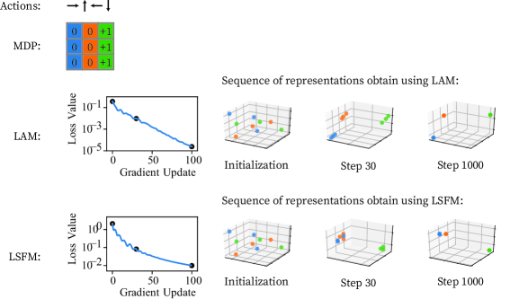
Refer to caption
Figure 5: In the column world task, learning reward-predictive state representations leads to clustering grid cells by each column. The top row illustrates a map of the column world task and a colouring of each column. The middle row presents an experiment that optimizes across different state representations to find a LAM that can be used for accurate one-step reward and one-step expected transition predictions. Each latent state is plotted as a dot in 3D-space and dots are coloured by the column they correspond to. At the end of the optimization process, three clusters of the same colour are formed showing that approximately the same latent state is assigned to states of the same column. The third row repeats the same experiment using an LSFM, which assesses whether the constructed latent state space can be used for accurate one-step reward predictions and SF predictions. Appendix C.1 describes this experiment in detail.

Using the previously presented theoretical results, this section designs a loss objective to learn approximate reward-predictive state representations. By optimizing a loss function, a randomly chosen state-representation function ϕ:𝒮n:italic-ϕ𝒮superscript𝑛\phi:\mathcal{S}\to\mathbb{R}^{n} is iteratively improved until the function ϕitalic-ϕ\phi can be used to accurately predict future reward sequences. The cluster plots in Figure 5 illustrate this process: Starting with a random assignment of feature vectors to different grid states, a state representation is iteratively improved until all states of the same column are clustered approximately into the same latent state. These latent state vectors were only clustered because the loss function assesses whether a state representation is reward predictive. The fact that states of the same column are assigned approximately to the same latent state is an artifact of this optimization process. The hyper-parameter n𝑛n can be understood as the size of the constructed latent space and a bound on the degree of compression of the state space. For example, if the state space consists of nine different states, setting n=9𝑛9n=9 could result in not compressing the state space and mapping nine states onto nine distinct one-hot bit vectors. The following experiments explore how choosing a low enough feature dimension leads to compression and generalization across states.

The previous sections present bounds on prediction errors that are parametrized in the worst-case one-step reward-prediction error εrsubscript𝜀𝑟\varepsilon_{r} and worst-case linear SF prediction error εψsubscript𝜀𝜓\varepsilon_{\psi}. Given only a finite data set of transitions 𝒟={(si,ai,ri,si)}i=1D𝒟superscriptsubscriptsubscript𝑠𝑖subscript𝑎𝑖subscript𝑟𝑖superscriptsubscript𝑠𝑖𝑖1𝐷\mathcal{D}=\left\{(s_{i},a_{i},r_{i},s_{i}^{\prime})\right\}_{i=1}^{D}, it may not be possible to compute estimates for εrsubscript𝜀𝑟\varepsilon_{r} and εψsubscript𝜀𝜓\varepsilon_{\psi} without making further assumptions on the MDP at hand, such as a finite state space or a bounded Rademacher complexity of the transition and reward functions to obtain robust performance on a test data set (Mohri et al., 2018). Because the goal of this project is to study the connections between SFs and different models of generalization across different states, an analysis of how to find provably correct predictions of εrsubscript𝜀𝑟\varepsilon_{r} and εψsubscript𝜀𝜓\varepsilon_{\psi} given a finite data set 𝒟𝒟\mathcal{D} is beyond the scope of this article. Instead, the conducted experiments collect a data set 𝒟𝒟\mathcal{D} by sampling trajectories using a policy that selects actions uniformly at random. The data set 𝒟𝒟\mathcal{D} is generated to be large enough to cover all state and action pairs, ensuring that all possible transitions and rewards are implicitly represented in this data set. If the data set does not cover all states and actions, then the resulting reward-predictive state representation may only produce accurate predictions for some reward sequences because the data set does not communicate all aspects of the MDP at hand. A study of this interaction between a possibly limited training data set and the resulting model’s ability to make accurate predictions is left for future work.

We design a loss objective to learn LSFMs LSFMsubscriptLSFM\mathcal{L}_{\text{LSFM}} that is the sum of three different terms: The first term rsubscript𝑟\mathcal{L}_{r} computes the one-step reward prediction error and is designed to minimize the reward error εrsubscript𝜀𝑟\varepsilon_{r}. The second term ψsubscript𝜓\mathcal{L}_{\psi} computes the SF prediction error and is designed to minimize the SF error εψsubscript𝜀𝜓\varepsilon_{\psi}. The last term Nsubscript𝑁\mathcal{L}_{N} is a regularizer constraining the gradient optimizer to find a state representation that outputs unit norm vectors. Empirically, we found that this regularizer encourages the optimizer to find a model with M1𝑀1M\approx 1 and W1𝑊1W\approx 1. (Reward-sequence prediction errors are lower for these values of M𝑀M and W𝑊W, as stated in Theorem 29.) Given a finite data set of transitions 𝒟={(si,ai,ri,si)}i=1D𝒟superscriptsubscriptsubscript𝑠𝑖subscript𝑎𝑖subscript𝑟𝑖superscriptsubscript𝑠𝑖𝑖1𝐷\mathcal{D}=\left\{(s_{i},a_{i},r_{i},s_{i}^{\prime})\right\}_{i=1}^{D}, the formal loss objective is

LSFM=i=1D(ϕsi𝒘airi)2=r+αψi=1Dϕsi𝑭a𝒚si,ai,ri,si22=ψ+αNi=1D(ϕsi221)2=N,subscriptLSFMsubscriptsuperscriptsubscript𝑖1𝐷superscriptsuperscriptsubscriptbold-italic-ϕsubscript𝑠𝑖topsubscript𝒘subscript𝑎𝑖subscript𝑟𝑖2absentsubscript𝑟subscript𝛼𝜓subscriptsuperscriptsubscript𝑖1𝐷superscriptsubscriptnormsuperscriptsubscriptbold-italic-ϕsubscript𝑠𝑖topsubscript𝑭𝑎subscript𝒚subscript𝑠𝑖subscript𝑎𝑖subscript𝑟𝑖superscriptsubscript𝑠𝑖22absentsubscript𝜓subscript𝛼𝑁subscriptsuperscriptsubscript𝑖1𝐷superscriptsuperscriptsubscriptnormsubscriptbold-italic-ϕsubscript𝑠𝑖2212absentsubscript𝑁\mathcal{L}_{\text{LSFM}}=\underbrace{\sum_{i=1}^{D}\Big{(}\boldsymbol{\phi}_{s_{i}}^{\top}\boldsymbol{w}_{a_{i}}-r_{i}\Big{)}^{2}}_{=\mathcal{L}_{r}}+\alpha_{\psi}\underbrace{\sum_{i=1}^{D}\Big{|}\Big{|}\boldsymbol{\phi}_{s_{i}}^{\top}\boldsymbol{F}_{a}-\vec{\boldsymbol{y}}_{s_{i},a_{i},r_{i},s_{i}^{\prime}}\Big{|}\Big{|}_{2}^{2}}_{=\mathcal{L}_{\psi}}+\alpha_{N}\underbrace{\sum_{i=1}^{D}\Big{(}\Big{|}\Big{|}\boldsymbol{\phi}_{s_{i}}\Big{|}\Big{|}_{2}^{2}-1\Big{)}^{2}}_{=\mathcal{L}_{N}}, (31)

for a finite data set of transitions 𝒟={(si,ai,ri,si)}i=1D𝒟superscriptsubscriptsubscript𝑠𝑖subscript𝑎𝑖subscript𝑟𝑖superscriptsubscript𝑠𝑖𝑖1𝐷\mathcal{D}=\left\{(s_{i},a_{i},r_{i},s_{i}^{\prime})\right\}_{i=1}^{D}. In Equation (31), the prediction target

𝒚s,a,r,s=ϕs+γϕs𝑭¯subscript𝒚𝑠𝑎𝑟superscript𝑠superscriptsubscriptbold-italic-ϕ𝑠top𝛾superscriptsubscriptbold-italic-ϕsuperscript𝑠top¯𝑭\vec{\boldsymbol{y}}_{s,a,r,s^{\prime}}=\boldsymbol{\phi}_{s}^{\top}+\gamma\boldsymbol{\phi}_{s^{\prime}}^{\top}\overline{\boldsymbol{F}}

and αψ,αN>0subscript𝛼𝜓subscript𝛼N0\alpha_{\psi},\alpha_{\text{N}}>0 are hyper-parameters. These hyper-parameters weigh the contribution of each error term to the overall loss objective. If αψsubscript𝛼𝜓\alpha_{\psi} is set to too small a value, then the resulting state representation may only produce accurate one-step reward predictions, but not accurate predictions of longer reward sequences. This article presents simulations on finite state spaces and represents a state representation as a function s𝒆s𝚽maps-to𝑠superscriptsubscript𝒆𝑠top𝚽s\mapsto\boldsymbol{e}_{s}^{\top}\boldsymbol{\Phi} where 𝚽𝚽\boldsymbol{\Phi} is a weight matrix of size |𝒮|×n𝒮𝑛|\mathcal{S}|\times n. An approximation of a reward-predictive state representation is obtained by performing gradient descent on the loss objective LSFMsubscriptLSFM\mathcal{L}_{\text{LSFM}} with respect to the free parameters {𝑭a,𝒘a}a𝒜subscriptsubscript𝑭𝑎subscript𝒘𝑎𝑎𝒜\{\boldsymbol{F}_{a},\boldsymbol{w}_{a}\}_{a\in\mathcal{A}} and 𝚽𝚽\boldsymbol{\Phi}. For each gradient update, the target 𝒚s,a,r,ssubscript𝒚𝑠𝑎𝑟superscript𝑠\vec{\boldsymbol{y}}_{s,a,r,s^{\prime}} is considered a constant. The previously presented bounds show that prediction errors also increase with Δ=maxa𝑰+γ𝑴a𝑭¯𝑭aΔsubscript𝑎norm𝑰𝛾subscript𝑴𝑎¯𝑭subscript𝑭𝑎\Delta=\max_{a}||\boldsymbol{I}+\gamma\boldsymbol{M}_{a}\overline{\boldsymbol{F}}-\boldsymbol{F}_{a}||. Minimizing ψsubscript𝜓\mathcal{L}_{\psi} for a fixed state representation ϕitalic-ϕ\phi minimizes ΔΔ\Delta, because

Δcϕψ,Δsubscript𝑐italic-ϕsubscript𝜓\Delta\leq c_{\phi}\mathcal{L}_{\psi}, (32)

where cϕsubscript𝑐italic-ϕc_{\phi} is a non-negative constant. Appendix A.3 presents a formal proof for Equation (32).
Refer to caption
(a) Puddle-world task map
Refer to caption
(b) LAM generalization map
Refer to caption
(c) LSFM generalization map
Refer to caption
(d) Example Rollout, Random
Refer to caption
(e) Example Rollout, LAM
Refer to caption
(f) Example Rollout, LSFM
Refer to caption
(g) Reward-Prediction Error
Refer to caption
(h) LAM Value-Prediction Error
Refer to caption
(i) LSFM Value-Prediction Error
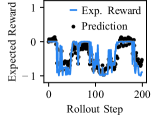
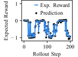
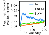
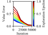
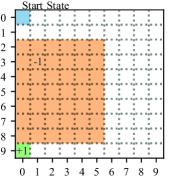
Figure 6: Puddle-World Experiment. 6(a): Map of the puddle-world task in which the agent can move up, down, left, or right to transition to adjacent grid cells. The agent always starts at the blue start cell and once the green reward cell is reached a reward of +11+1 is given and the interaction sequence is terminated. For each transition that enters the orange puddle, a reward of 11-1 is received. 6(b)6(c): Partitioning obtained by merging latent states into clusters by Euclidean distance. 6(d)6(e)6(f): Expected reward and predictions for a randomly chosen 200-step action sequence using a randomly chosen representation, a representation learned with a LAM, and a representation learned with an LSFM. 6(g): Average expected reward-prediction errors with standard error for each representation. 6(h)6(i): Optimizing the loss objective results in a sequence of state representations suitable for finding linear approximations of the value functions for a range of different ε𝜀\varepsilon-greedy policies. Appendix C.2 presents more details.

To assess whether minimizing the loss LSFMsubscriptLSFM\mathcal{L}_{\text{LSFM}} leads to approximating reward-predictive state representations, a transition data set was collected from the puddle-world task (Boyan and Moore, 1995). Conforming to the previous analysis, the LSFM is compared to a LAM that is trained using a similar loss function, described in Appendix C.2.

Figure 6 presents the puddle-world experiments and the results. In puddle-world (Figure 6(a)), the agent has to navigate from a start state to a goal to obtain a reward of one while avoiding a puddle. Entering the puddle is penalized with a reward of minus one. To predict future reward outcomes accurately, a state representation has to preserve the grid position as accurately as possible to predict the location of the different reward cells.

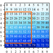
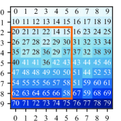
By constraining the latent state space to 80 dimensions, the optimization process is forced to find a compression of all 100 grid cells. To analyze across which states the learned reward-predictive state representation generalizes, all feature vectors were clustered using agglomerative clustering. Two different states that are associated with feature vectors ϕssubscriptbold-italic-ϕ𝑠\boldsymbol{\phi}_{s} and ϕs~subscriptbold-italic-ϕ~𝑠\boldsymbol{\phi}_{\tilde{s}} are merged into the same cluster if their Euclidean distance ϕsϕs~2subscriptnormsubscriptbold-italic-ϕ𝑠subscriptbold-italic-ϕ~𝑠2||\boldsymbol{\phi}_{s}-\boldsymbol{\phi}_{\tilde{s}}||_{2} is low. For example, a randomly chosen representation would randomly assign states to different latent states and the partition map could assign the grid cell at (0,0)00(0,0) and (9,9)99(9,9) to the same latent state. Figures 6(b) and 6(c) plot the obtained clustering as a partition map. Grid cells are labelled with the same partition index if they belong to the same cluster and colours correspond to the partition index. To predict reward outcomes accurately, the position in the grid needs to be roughly retained in the constructed latent state space. The partition maps in Figures 6(b) and 6(c) suggest that the learned state representation extracts this property from a transition data set, by generalizing only across neighboring grid cells and tiling the grid space. Only a transition data set 𝒟𝒟\mathcal{D} was given as input to the optimization algorithm and the algorithm was not informed about the grid-world topology of the task in any other way.

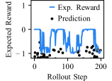
Figures 6(d)6(e)6(f) plot an expected reward rollout and the predictions presented by a random initialization (6(d)), the learned representation using a LAM (6(e)), and the learned representation using a LSFM (6(f)). The blue curve plots the expected reward outcome 𝔼p[rt|s,a1,,at]subscript𝔼𝑝delimited-[]conditionalsubscript𝑟𝑡𝑠subscript𝑎1subscript𝑎𝑡\mathbb{E}_{p}[r_{t}|s,a_{1},...,a_{t}] as a function of t𝑡t for a randomly selected action sequence. Because transitions are probabilistic, the (blue) expected reward curve is smoothed and does not assume exact values of 11-1 or +11+1. While a randomly initialized state representation produces poor predictions of future reward outcomes (Figures 6(d)), the learned representations produce relatively accurate predictions and follow the expected reward curve (Figures 6(e) and 6(f)). Because the optimization process was forced to compress 100 grid cells into a 80-dimensional latent state space, the latent state space cannot preserve the exact grid cell position and thus approximation errors occur.

Figure 6(g) averages the expected reward-prediction errors across 100 randomly selected action sequences. While a randomly chosen initialization produces high prediction errors, the learned state representations produce relatively low prediction errors of future reward outcomes. If expected reward-prediction errors are random after 200 time steps, then the γ𝛾\gamma-discounted return can be off by at most 0.92001/(10.9)1.4109superscript0.9200110.91.4superscript1090.9^{200}\cdot 1/(1-0.9)\approx 1.4\cdot 10^{-9} after 200 time steps for γ=0.9𝛾0.9\gamma=0.9 and a reward range of [1,1]11[-1,1]. Hence, planning over a horizon of more than 200 time steps will impact a policy’s value estimate insignificantly. Reward-prediction errors decrease for a randomly chosen state representation (blue curve in Figure 6(g)) because the stochasticity of the task’s transitions smooths future expected reward outcomes as the number of steps increases.

While the plots in Figure 6 suggest that both LSFMs and LAMs can be used to learn approximate reward-predictive state representations, the LSFM produces lower prediction errors for expected reward outcomes than the LAM and the LAM produces lower value-prediction errors. Because both models optimize different non-linear and non-convex loss functions, the optimization process leads to different local optima, leading to different performance on the puddle-world task. While prediction errors are present, Figure 6 suggests that both LSFM and LAM learn an approximate reward-predictive state representation and empirically the differences between each model are not significant.

4.4 Connection to Model-based Reinforcement Learning

The key characteristic of a model-based RL agent is to build an internal model of a task that supports predictions of future reward outcomes for any arbitrary decision sequence. Because reward-predictive state representations construct a latent state space suitable for predicting reward sequences for any arbitrary decision sequence, learning reward-predictive state representations can be understood as form of model-based RL. LSFMs tie SFs to reward-predictive state representations, which support predictions of future reward outcomes for any arbitrary decision sequence. The presented analysis describes how learning SFs is akin to learning a transition and reward model in model-based RL.

5 Connections to Value-Predictive Representations

This section first outlines how SFs are related to value-predictive state representations and how learning SFs is akin to model-free learning. Subsequently, we illustrate how reward-predictive state representations can be re-used across tasks with different transitions and rewards to find an optimal policy while re-using value-predictive state representations may prohibit an agent from learning an optimal policy. Barreto et al. (2017a) present SFs as a factorization of the Q-value function for an arbitrary fixed policy π𝜋\pi and demonstrate that re-using SFs across tasks with different reward functions improves the convergence rate of online learning algorithms. This factorization assumes a state and action representation function ξ:𝒮×𝒜m:𝜉𝒮𝒜superscript𝑚\xi:\mathcal{S}\times\mathcal{A}\to\mathbb{R}^{m} that serves as a basis function for one-step reward predictions and

s𝒮,a𝒜,𝝃s,a𝒘=𝔼p[r(s,a,s)|s,a].\forall s\in\mathcal{S},~{}\forall a\in\mathcal{A},~{}\boldsymbol{\xi}_{s,a}^{\top}\boldsymbol{w}=\mathbb{E}_{p}\left[r(s,a,s^{\prime})\middle|s,a\right]. (33)

Using a state and action representation function, the Q-value function can be factored:

Qπ(s,a)superscript𝑄𝜋𝑠𝑎\displaystyle Q^{\pi}(s,a) =𝔼p,π[t=1γt1r(st,at,st+1)|s1=s,a1=a]\displaystyle=\mathbb{E}_{p,\pi}\left[\sum_{t=1}^{\infty}\gamma^{t-1}r(s_{t},a_{t},s_{t+1})\middle|s_{1}=s,a_{1}=a\right] (34)
=𝔼p,π[t=1γt1𝝃st,at𝒘|s1=s,a1=a]\displaystyle=\mathbb{E}_{p,\pi}\left[\sum_{t=1}^{\infty}\gamma^{t-1}\boldsymbol{\xi}_{s_{t},a_{t}}^{\top}\boldsymbol{w}\middle|s_{1}=s,a_{1}=a\right] (by (33))by (33)\displaystyle(\text{by~{}\eqref{eq:r-def}}) (35)
=𝔼p,π[t=1γt1𝝃st,at|s1=s,a1=a]𝒘\displaystyle=\mathbb{E}_{p,\pi}\left[\sum_{t=1}^{\infty}\gamma^{t-1}\boldsymbol{\xi}_{s_{t},a_{t}}^{\top}\middle|s_{1}=s,a_{1}=a\right]\boldsymbol{w} (36)
=(𝝍SAπ(s1,a1))𝒘.absentsuperscriptsuperscriptsubscript𝝍SA𝜋subscript𝑠1subscript𝑎1top𝒘\displaystyle=\left(\boldsymbol{\psi}_{\text{SA}}^{\pi}(s_{1},a_{1})\right)^{\top}\boldsymbol{w}. (where s1=sa1=a)where s1=sa1=a\displaystyle(\text{where $s_{1}=s$, $a_{1}=a$}) (37)

Equation (37) assumes the following definition for a SF ψSAπsuperscriptsubscript𝜓SA𝜋\psi_{\text{SA}}^{\pi}:

𝝍SAπ(s,a)=def.𝔼p,π[t=1γt1𝝃st,at|s1=s,a1=a].\boldsymbol{\psi}_{\text{SA}}^{\pi}(s,a)\overset{\text{def.}}{=}\mathbb{E}_{p,\pi}\left[\sum_{t=1}^{\infty}\gamma^{t-1}\boldsymbol{\xi}_{s_{t},a_{t}}\middle|s_{1}=s,a_{1}=a\right]. (38)

The state and action SF 𝝍SAπsuperscriptsubscript𝝍SA𝜋\boldsymbol{\psi}_{\text{SA}}^{\pi} is a basis function that allows accurate predictions of the Q-value function Qπsuperscript𝑄𝜋Q^{\pi}. Consequently, the representation 𝝍SAπsuperscriptsubscript𝝍SA𝜋\boldsymbol{\psi}_{\text{SA}}^{\pi} is a value-predictive state representation because it is designed to construct a latent feature space that supports accurate predictions of the Q-value function Qπsuperscript𝑄𝜋Q^{\pi}.

A𝐴A B𝐵B C𝐶C D𝐷D a,b,r=0.5𝑎𝑏𝑟0.5a,b,r=0.5a,r=1𝑎𝑟1a,r=1b,r=0𝑏𝑟0b,r=0b,r=0𝑏𝑟0b,r=0a,r=0𝑎𝑟0a,r=0b,r=0𝑏𝑟0b,r=0a,r=0𝑎𝑟0a,r=0Value predictive:Qπ¯(A,a)=γ1γ0.5superscript𝑄¯𝜋𝐴𝑎𝛾1𝛾0.5Q^{\overline{\pi}}(A,a)=\color[rgb]{0.12109375,0.46484375,0.70703125}\definecolor[named]{pgfstrokecolor}{rgb}{0.12109375,0.46484375,0.70703125}\frac{\gamma}{1-\gamma}0.5Qπ¯(A,b)=γ1γ0.5superscript𝑄¯𝜋𝐴𝑏𝛾1𝛾0.5Q^{\overline{\pi}}(A,b)=\color[rgb]{0.12109375,0.46484375,0.70703125}\definecolor[named]{pgfstrokecolor}{rgb}{0.12109375,0.46484375,0.70703125}\frac{\gamma}{1-\gamma}0.5Qπ¯(B,a)=γ1γ0.5superscript𝑄¯𝜋𝐵𝑎𝛾1𝛾0.5Q^{\overline{\pi}}(B,a)=\color[rgb]{0.12109375,0.46484375,0.70703125}\definecolor[named]{pgfstrokecolor}{rgb}{0.12109375,0.46484375,0.70703125}\frac{\gamma}{1-\gamma}0.5Qπ¯(B,b)=γ1γ0.5superscript𝑄¯𝜋𝐵𝑏𝛾1𝛾0.5Q^{\overline{\pi}}(B,b)=\color[rgb]{0.12109375,0.46484375,0.70703125}\definecolor[named]{pgfstrokecolor}{rgb}{0.12109375,0.46484375,0.70703125}\frac{\gamma}{1-\gamma}0.5Reward predictive:𝝍π¯(A,a)=ϕA+11γϕDsuperscript𝝍¯𝜋𝐴𝑎subscriptbold-italic-ϕ𝐴11𝛾subscriptbold-italic-ϕ𝐷\boldsymbol{\psi}^{\overline{\pi}}(A,a)=\boldsymbol{\phi}_{A}+\color[rgb]{0.171875,0.62890625,0.171875}\definecolor[named]{pgfstrokecolor}{rgb}{0.171875,0.62890625,0.171875}\frac{1}{1-\gamma}\boldsymbol{\phi}_{D}𝝍π¯(A,b)=ϕA+11γϕCsuperscript𝝍¯𝜋𝐴𝑏subscriptbold-italic-ϕ𝐴11𝛾subscriptbold-italic-ϕ𝐶\boldsymbol{\psi}^{\overline{\pi}}(A,b)=\boldsymbol{\phi}_{A}+\color[rgb]{1,0.49609375,0.0546875}\definecolor[named]{pgfstrokecolor}{rgb}{1,0.49609375,0.0546875}\frac{1}{1-\gamma}\boldsymbol{\phi}_{C}𝝍π¯(B,a)=ϕB+11γϕCsuperscript𝝍¯𝜋𝐵𝑎subscriptbold-italic-ϕ𝐵11𝛾subscriptbold-italic-ϕ𝐶\boldsymbol{\psi}^{\overline{\pi}}(B,a)=\boldsymbol{\phi}_{B}+\color[rgb]{1,0.49609375,0.0546875}\definecolor[named]{pgfstrokecolor}{rgb}{1,0.49609375,0.0546875}\frac{1}{1-\gamma}\boldsymbol{\phi}_{C}𝝍π¯(B,b)=ϕB+11γϕDsuperscript𝝍¯𝜋𝐵𝑏subscriptbold-italic-ϕ𝐵11𝛾subscriptbold-italic-ϕ𝐷\boldsymbol{\psi}^{\overline{\pi}}(B,b)=\boldsymbol{\phi}_{B}+\color[rgb]{0.171875,0.62890625,0.171875}\definecolor[named]{pgfstrokecolor}{rgb}{0.171875,0.62890625,0.171875}\frac{1}{1-\gamma}\boldsymbol{\phi}_{D}
Figure 7: Value-predictive state representations may prohibit an agent from learning an optimal policy. In this MDP, the agent can choose between action a𝑎a and action b𝑏b. All transitions are deterministic and each edge is labelled with the reward given to the agent. If a uniform-random action-selection policy is used to construct a value-predictive state representation, then both states A𝐴A and B𝐵B will have equal Q-values. A reward-predictive state representation would always distinguish between A𝐴A and B𝐵B, because at state A𝐴A the action sequence b,a,a𝑏𝑎𝑎b,a,a... leads to a reward sequence of 0,0.5,0.5,00.50.50,0.5,0.5,... while at state B𝐵B the action sequence b,a,a,𝑏𝑎𝑎b,a,a,... leads to a reward sequence of 0,1,1,0110,1,1,.... An LSFM detects that states A𝐴A and B𝐵B should not be merged into the same latent state, because the states have different SFs. The optimal policy is to select action a𝑎a at state A𝐴A, and action b𝑏b at state B𝐵B and then collect a reward of one at state D𝐷D by repeating action a𝑎a. If an agent uses a reward-predictive state representation, then the optimal policy could be recovered. If an agent uses a value-predictive state representation, the agent would be constrained to not distinguish between states A𝐴A and B𝐵B and cannot recover an optimal policy.

Figure 7 illustrates that value-predictive state representations generalize across different states differently than reward-predictive state representations. The counter example presented in Figure 7 demonstrates that it is not always possible to construct an optimal policy using a value-predictive state representation. If a sub-optimal policy is used, value-predictive state representations may alias states that have different optimal actions prohibiting an intelligent agent from finding an optimal policy. In this case the value-predictive state representation has to be adjusted for the agent to be able to find an optimal policy, a phenomenon that has been previously described by Russek et al. (2017). In contrast, reward-predictive state representations generalize across the entire policy space (Theorem 4) and allow an agent to find either an optimal policy or close to optimal policy in the presence of approximation errors.

In the following section, we show that learning SFs is akin to learning a value function in model-free RL and the presented argument ties SFs to model-free RL. Subsequently, we demonstrate that reward-predictive state representations can be re-used across tasks with different transitions and rewards to find an optimal policy on two transfer examples in Sections 5.2 and 5.3. While value-predictive state representations may prohibit an agent from learning an optimal policy (Figure 7), we illustrate in which cases reward-predictive state representations overcome this limitation.

5.1 Connection to Linear Temporal Difference Learning

Algorithms that learn SFs can be derived similarly to linear TD-learning (Sutton and Barto, 1998, Chapter 8.4). In linear TD-learning algorithms such as linear Q-learning or SARSA, all Q-values are represented with

Qπ(s,a;𝜽)=𝝃s,a𝜽,superscript𝑄𝜋𝑠𝑎𝜽superscriptsubscript𝝃𝑠𝑎top𝜽Q^{\pi}(s,a;\boldsymbol{\theta})=\boldsymbol{\xi}_{s,a}^{\top}\boldsymbol{\theta}, (39)

where 𝜽𝜽\boldsymbol{\theta} is a real-valued weight vector that does not depend on a state s𝑠s or action a𝑎a. Linear TD-learning learns the parameter vector 𝜽𝜽\boldsymbol{\theta} by minimizing the mean squared value error

VE(𝜽)=s,a,r,sμ(s,a,r,s)(Q𝜽π(s,a;𝜽)ys,a,r,s)2.VE𝜽subscript𝑠𝑎𝑟superscript𝑠𝜇𝑠𝑎𝑟superscript𝑠superscriptsuperscriptsubscript𝑄𝜽𝜋𝑠𝑎𝜽subscript𝑦𝑠𝑎𝑟superscript𝑠2\text{VE}(\boldsymbol{\theta})=\sum_{s,a,r,s^{\prime}}\mu(s,a,r,s^{\prime})\left(Q_{\boldsymbol{\theta}}^{\pi}(s,a;\boldsymbol{\theta})-y_{s,a,r,s^{\prime}}\right)^{2}. (40)

Equation (40) averages prediction errors with respect to some distribution μ𝜇\mu with which transitions (s,a,r,s)𝑠𝑎𝑟superscript𝑠(s,a,r,s^{\prime}) are sampled. The prediction target

ys,a,r,s=r+γab(s,a)Qπ(s,a;𝜽)subscript𝑦𝑠𝑎𝑟superscript𝑠𝑟𝛾subscriptsuperscript𝑎𝑏superscript𝑠superscript𝑎superscript𝑄𝜋superscript𝑠superscript𝑎𝜽y_{s,a,r,s^{\prime}}=r+\gamma\sum_{a^{\prime}}b(s^{\prime},a^{\prime})Q^{\pi}(s^{\prime},a^{\prime};\boldsymbol{\theta}) (41)

varies by which function b𝑏b is used. For example, to find the optimal policy linear Q-learning uses an indicator function b(s,a)=𝟏[a=argmaxaQπ(s,a;𝜽)]𝑏𝑠𝑎1delimited-[]𝑎subscript𝑎superscript𝑄𝜋𝑠𝑎𝜽b(s,a)=\boldsymbol{1}[a=\arg\max_{a}Q^{\pi}(s,a;\boldsymbol{\theta})] so that ys,a,r,s=r+γmaxaQπ(s,a;𝜽)subscript𝑦𝑠𝑎𝑟superscript𝑠𝑟𝛾subscriptsuperscript𝑎superscript𝑄𝜋superscript𝑠superscript𝑎𝜽y_{s,a,r,s^{\prime}}=r+\gamma\max_{a^{\prime}}Q^{\pi}(s^{\prime},a^{\prime};\boldsymbol{\theta}). For Expected SARSA (Sutton and Barto, 2018, Chapter 6.6), which evaluates a fixed policy π𝜋\pi, the target can be constructed using b(s,a)=π(s,a)𝑏𝑠𝑎𝜋𝑠𝑎b(s,a)=\pi(s,a), where π(s,a)𝜋𝑠𝑎\pi(s,a) specifies the probability with which a𝑎a is selected at state s𝑠s. When computing a gradient of VE(𝜽)VE𝜽\text{VE}(\boldsymbol{\theta}) the prediction target ys,a,r,ssubscript𝑦𝑠𝑎𝑟superscript𝑠y_{s,a,r,s^{\prime}} is considered a constant. For an observed transition (s,a,r,s)𝑠𝑎𝑟superscript𝑠(s,a,r,s^{\prime}), the parameter vector is updated using the rule

𝜽t+1=𝜽t+α(Qπ(s,a;𝜽t)ys,a,r,s)𝝃s,a,subscript𝜽𝑡1subscript𝜽𝑡𝛼superscript𝑄𝜋𝑠𝑎subscript𝜽𝑡subscript𝑦𝑠𝑎𝑟superscript𝑠subscript𝝃𝑠𝑎\boldsymbol{\theta}_{t+1}=\boldsymbol{\theta}_{t}+\alpha\left(Q^{\pi}(s,a;\boldsymbol{\theta}_{t})-y_{s,a,r,s^{\prime}}\right)\boldsymbol{\xi}_{s,a}, (42)

where α𝛼\alpha is a learning rate and the subscript t𝑡t tracks the update iteration. A SF-learning algorithm can be derived by defining the mean squared SF error (Lehnert et al., 2017)

SFE(𝝍SAπ)=s,a,r,sμ(s,a,r,s)𝝍SAπ(s,a)𝒚s,a,r,s2.SFEsubscriptsuperscript𝝍𝜋SAsubscript𝑠𝑎𝑟superscript𝑠𝜇𝑠𝑎𝑟superscript𝑠superscriptnormsubscriptsuperscript𝝍𝜋SA𝑠𝑎subscript𝒚𝑠𝑎𝑟superscript𝑠2\text{SFE}(\boldsymbol{\psi}^{\pi}_{\text{SA}})=\sum_{s,a,r,s^{\prime}}\mu(s,a,r,s^{\prime})||\boldsymbol{\psi}^{\pi}_{\text{SA}}(s,a)-\vec{\boldsymbol{y}}_{s,a,r,s^{\prime}}||^{2}. (43)

Because the SF 𝝍SAπ(s,a)subscriptsuperscript𝝍𝜋SA𝑠𝑎\boldsymbol{\psi}^{\pi}_{\text{SA}}(s,a) is a vector of dimension m𝑚m, the target

𝒚s,a,r,s=𝝃s,a+γab(s,a)𝝍SAπ(s,a)subscript𝒚𝑠𝑎𝑟superscript𝑠subscript𝝃𝑠𝑎𝛾subscriptsuperscript𝑎𝑏superscript𝑠superscript𝑎subscriptsuperscript𝝍𝜋SAsuperscript𝑠superscript𝑎\vec{\boldsymbol{y}}_{s,a,r,s^{\prime}}=\boldsymbol{\xi}_{s,a}+\gamma\sum_{a^{\prime}}b(s^{\prime},a^{\prime})\boldsymbol{\psi}^{\pi}_{\text{SA}}(s^{\prime},a^{\prime}) (44)

is also a vector but can be constructed similarly to the usual value-prediction target ys,a,r,ssubscript𝑦𝑠𝑎𝑟superscript𝑠y_{s,a,r,s^{\prime}}. Assuming that SFs are approximated linearly using the basis function ξ𝜉\xi,

𝝍SAπ(s,a;𝑮)=𝑮𝝃s,a,subscriptsuperscript𝝍𝜋SA𝑠𝑎𝑮𝑮subscript𝝃𝑠𝑎\boldsymbol{\psi}^{\pi}_{\text{SA}}(s,a;\boldsymbol{G})=\boldsymbol{G}\boldsymbol{\xi}_{s,a}, (45)

where 𝑭𝑭\boldsymbol{F} is a square matrix. Computing the gradient of SFE(𝝍π)SFEsuperscript𝝍𝜋\text{SFE}(\boldsymbol{\psi}^{\pi}) with respect to 𝑭𝑭\boldsymbol{F} results in an update rule similar to linear TD-learning:

𝑮t+1=𝑮t+α(𝝍SAπ(s,a;𝑮t)𝒚s,a,r,s)𝝃s,a.subscript𝑮𝑡1subscript𝑮𝑡𝛼subscriptsuperscript𝝍𝜋SA𝑠𝑎subscript𝑮𝑡subscript𝒚𝑠𝑎𝑟superscript𝑠superscriptsubscript𝝃𝑠𝑎top\boldsymbol{G}_{t+1}=\boldsymbol{G}_{t}+\alpha\left(\boldsymbol{\psi}^{\pi}_{\text{SA}}(s,a;\boldsymbol{G}_{t})-\vec{\boldsymbol{y}}_{s,a,r,s^{\prime}}\right)\boldsymbol{\xi}_{s,a}^{\top}. (46)

Assuming the reward condition in Equation (33) holds, both linear TD-learning and SF-learning produce the same value-function sequence.

Proposition 1 (Linear TD-learning and SF-learning Equivalence).

Consider an MDP and a basis function ξ𝜉\xi such that r(s,a)=𝛏s,a𝐰𝑟𝑠𝑎superscriptsubscript𝛏𝑠𝑎top𝐰r(s,a)=\boldsymbol{\xi}_{s,a}^{\top}\boldsymbol{w} for all states s𝑠s and actions a𝑎a. Suppose both iterates in Equation (42) and in Equation (46) use the same function b𝑏b to construct prediction targets and are applied for the same trajectory (s1,a1,r1,s2,a2,)subscript𝑠1subscript𝑎1subscript𝑟1subscript𝑠2subscript𝑎2(s_{1},a_{1},r_{1},s_{2},a_{2},...). If 𝛉0=𝐆0𝐰subscript𝛉0subscript𝐆0𝐰\boldsymbol{\theta}_{0}=\boldsymbol{G}_{0}\boldsymbol{w}, then

t>0,𝜽t=𝑮t𝒘.formulae-sequencefor-all𝑡0subscript𝜽𝑡subscript𝑮𝑡𝒘\forall t>0,~{}\boldsymbol{\theta}_{t}=\boldsymbol{G}_{t}\boldsymbol{w}. (47)

Proposition 1 proves that both linear TD-learning and linear SF-learning generate identical value-function estimates on the same trajectory. Appendix B proves Proposition 1. Because linear TD-learning need not converge to an optimal solution, the SF iterate in Equation (46) also need not converge to an optimal solution. The tabular case, in which convergence can be guaranteed, is a sub-case of the presented analysis: For finite state and action spaces, a basis function ξ𝜉\xi can be constructed that outputs a one-hot bit vector of dimension n𝑛n, where n𝑛n is the number of all state and action pairs. In this case, each weight in the parameter vector 𝜽𝜽\boldsymbol{\theta} corresponds to the Q-value for a particular state and action pair. Similarly, each row in the matrix 𝑭𝑭\boldsymbol{F} corresponds to the SF vector for a particular state and action pair. In this light, learning SFs is akin to learning a value function in model-free RL.

5.2 Generalization Across Transition and Reward Functions

One key distinction between value- and reward-predictive state representations is their ability to generalize across different transition and reward functions. While prior work on SFs (Barreto et al., 2016) and adversarial IRL (Fu et al., 2018) separately model the reward function from the transition function and observed policy, reward-predictive state representations only model equivalence relations between states separately from the transition and reward model. Consequently, reward-predictive state representations extract equivalences between different state’s transitions and one-step rewards, reward-predictive state representations can be reused across tasks that vary in their transition and reward functions (Lehnert et al., 2019). Figure 8 presents a transfer experiment highligting that reusing a previously learned reward-predictive state representation allows an intelligent agent to learn an optimal policy using less data.

This experiment uses two grid-world tasks (Figure 8(a)): For Task A, a transition data set 𝒟Asubscript𝒟𝐴\mathcal{D}_{A} is collected. A reward-predictive state representation is learned using an LSFM and a value-predictive state representation is learned using a form of Fitted Q-iteration (Riedmiller, 2005). These state representations are then reused without modification to learn an optimal policy for Task B given a data set 𝒟Bsubscript𝒟𝐵\mathcal{D}_{B} collected from Task B. Both data sets are generated by performing a random walk from a uniformly sampled start state to one of the rewarding goal states. In both tasks, the agent can transition between adjacent grid cells by moving up, down, left, or right, but cannot transition across a barrier. Transitions are probabilistic, because, with a 5% chance, the agent does not move after selecting any action.

Figure 8(b) presents two heuristics for clustering all 100 states into 50 latent states. The first heuristic constructs a reward-predictive state representation by joining states into the same latent state partition if they are directly connected to another. Because both tasks are navigation tasks, partitioning the state space in this way leads to approximately perserving the agent’s location in the grid. The second heuristic constructs a value-predictive state representation by joining states that have approximately the same optimal Q-values. Because Q-values are discounted sums of rewards, Q-values decay as one moves further away from a goal cell. This situation leads to different corners being merged into the same state parition (for example grid cell (0,0)00(0,0) is merged with (0,9)09(0,9)) and an overall more fragmented partitioning that does not perserve the agent’s location. Because both state representations are computed for Task A, both state representations can be used to compute an optimal policy for Task A. For Task B, an optimal policy cannot be obtained using the value-predictive state representation. For example, both grid cells at (0,0)00(0,0) and (0,9)09(0,9) have different optimal actions in Task B but are mapped to the same latent state. Consequently, an optimal action cannot be computed using the previously learned value-predictive state representation. Because each grid cell has a different optimal action, an optimal abstract policy mapping each latent state to an optimal action cannot be found and the navigation Task B cannot be completed within 5000 time steps if the value-predictive state representation is used (Figure 8(b), right panel). In contrast, the reward-predictive state representation can be used, because it approximately models the grid-world topology. For Task B, each latent state has to be associated with different one-step rewards and latent transitions, but it is still possible to obtain an optimal policy using this state representation and complete the navigation task quickly.

Task A:Refer to captionTask B:Refer to caption: Start state: Goal state (+1 reward): Barrier
(a) Maps of Transfer Grid Worlds
Refer to captionRefer to captionRefer to caption Reward Predictive (Connected States) Value Predictive (App. Equal Qπsuperscript𝑄superscript𝜋Q^{\pi^{*}}) Performance in Task A Performance in Task B Simulations are repeated 20 times.
(b) State representations obtained using a clustering heuristic or optimal Q-values of Task A
Refer to captionRefer to captionRefer to caption Reward Predictive (LSFM) Value Predictive (Fitted Q) Data Set Size Needed to Solve Task B
(c) State partitions obtained through learning on a transition data set 𝒟𝒟\mathcal{D}.
Figure 8: Reward-predictive representations generalize across variations in transitions and rewards. 8(b): The left panels plot state partitions obtained by clustering connected states or states with equal optimal Q-values in Task A (8(a)). The right panels plot the number of times steps a policy, which uses each representation, needs to complete Task B (8(a)). 8(c): The left panels plot partitions obtained by clustering latent states of a reward-predictive and value-predictive representation. The right panel plots how often one out of 20 transition data sets can be used to find an optimal policy as a function of the data set size. By reusing the learned reward-predictive representation, an agent can generalize across states and compute an optimal policy using less data than a tabular model-based RL agent. Reusing a value-predictive representation leads to poor performance, because this representation is only predictive of Task A’s optimal policy.

Figure 8(c) repeats a similar experiment, but learns a state representation using either an LSFM to find a reward-predictive state representation or a modification of Fitted Q-iteration to find a value-predictive state representation. The two left panels in Figure 8(c) plot a partitioning of the state space that was obtained by clustering all latent state feature vectors using agglomerative clustering. In this experiment, the latent feature space was set to have 50 dimensions. One can observe that the state representation learned using an LSFM qualitatively corresponds to clustering connected grid cells. The learned value-predictive state representation qualitatively resembles a clustering of states by their optimal Q-values, because Fitted Q-iteration optimizes this state representation to predict the optimal value function as accurately as possible. Both state representations are tested on Task B using the following proceedure: First, a data set 𝒟Bsubscript𝒟𝐵\mathcal{D}_{B} was collected of a fixed size. Then, Fitted Q-iteration was used to compute the optimal policy for Task B using the previously learned state representation as a basis function such that Qπ(s,a)ϕs𝒒asuperscript𝑄superscript𝜋𝑠𝑎superscriptsubscriptbold-italic-ϕ𝑠topsubscript𝒒𝑎Q^{\pi^{*}}(s,a)\approx\boldsymbol{\phi}_{s}^{\top}\boldsymbol{q}_{a} where 𝒒asubscript𝒒𝑎\boldsymbol{q}_{a} is a weight vector and ϕ(s)=ϕsitalic-ϕ𝑠subscriptbold-italic-ϕ𝑠\phi(s)=\boldsymbol{\phi}_{s}. The state representation ϕitalic-ϕ\phi trained on Task A is not modified to obtain an optimal policy in Task B. If the training data set 𝒟Bsubscript𝒟𝐵\mathcal{D}_{B} obtained from Task B is too small, then the data set may not provide enough information to find an optimal policy. In this case, Fitted Q-iteration converged to a sub-optimal policy. Because the data sets 𝒟Bsubscript𝒟𝐵\mathcal{D}_{B} are generated at random, one may find that sampling a data set of 2000 transitions may lead to an optimal solution often, but not all the time.

The right panel in Figure 8(c) plots the dependency of being able to find an optimal policy as a function of the transition data set. For each data set size, twenty different data sets were sampled and the y-axis plots the fraction (with standard error of measure) of how often using this data set leads to a close-to-optimal policy. A close-to-optimal policy solves the navigation task in at most 22 time steps. The orange curve is computed using a tabular model-based agent, which constructs a transition and reward table using the sampled data set and solves for an optimal policy using value iteration. Reusing a reward-predictive state representation in Task B often leads to finding an optimal policy for small data set sizes (the blue curve in Figure 8(c), right panel). Because the training data set 𝒟Bsubscript𝒟𝐵\mathcal{D}_{B} is only used to inform different latent transitions and rewards, this agent can generalize across different states and reuse what it has learned without having to observe every possible transition. This behavior leads to better performance than the tabular model-based baseline algorithm, which does not generalize across different states and constructs a transition table for Task B and computes an optimal policy using value iteration (Sutton and Barto, 2018, Chapter 4.4). Reusing the learned value-predictive state representation leads to finding a sub-optimal policy in almost all cases (green curve in Figure 8(c), right panel). The value-predictive state representation is optimized to predict the Q-value function of the optimal policy in Task A. Because Task B has a different optimal policy, reusing this representation does not lead to an optimal policy in Task B, because the previously learned representation is explicitly tied to Task A’s optimal policy. Note that any trial that did not find a close-to-optimal policy that completes the task in 22 time steps did also not finish the task and hit the timeout threshold of 5000 time steps. Appendix C.3 presents additional details on the experiments conducted in Figure 8.

5.3 Reward-Predictive Representations Encode Task Relevant State Information

In this section, we present the last simulation result illustrating which aspect of an MDP reward-predictive state representations encode. Figure 9(a) illustrates the combination lock task, where an agent rotates three different numerical dials to obtain a rewarding number combination. In this task, the state is defined as a number triple and each dial has five different positions labelled with the digits zero through four. For example, if Action 1 is chosen at state (0,1,4)014(0,1,4), then the left dial rotates by one step and the state changes to (1,1,4)114(1,1,4). A dial that is set to four will rotate to zero. For example, selecting Action 2 at state (0,4,4)044(0,4,4) will result in a transition to state (0,0,4)004(0,0,4).

In the Training Lock task (Figure 9(a), left schematic), the right dial is “broken” and spins randomly after each time step. Consequently, Action 3 (red arrow) only causes a random change in the right dial and the agent can only use Action 1 (blue arrow) or Action 2 (green arrow) to manipulate the state of the lock. When the agent enters a combination where the left and middle dials are set to four, a reward of +11+1 is given, otherwise the agent receives no reward.777Specifically, in the Training Lock task, the rewarding states are (4,4,0),(4,4,1),(4,4,4)440441444(4,4,0),(4,4,1),\dots(4,4,4). While the combination lock task has 555=1255551255\cdot 5\cdot 5=125 different states, the state space of the Training Lock can be compressed to 55=2555255\cdot 5=25 latent states by ignoring the position of the randomly changing right dial, because the right dial is neither relevant for maximizing reward nor predicting reward sequences.

The Test Lock 1 and Test Lock 2 tasks (Figure 9(a), center and right schematics) differ from the training task in that the rewarding combination is changed and the rotation direction of the left dial is reversed (Action 1, blue arrow), resembling a change in both transition and reward functions. While in Test Lock 1, the right dial still spins at random, in Test Lock 2 the middle dial rotates at random instead and the right dial becomes relevant for maximizing reward. Both test tasks can also be compressed into 25 latent states by ignoring the position of the randomly rotating dial, but in Test Lock 2 this compression would be constructed differently than in Test Task 1 or in the Training Lock.

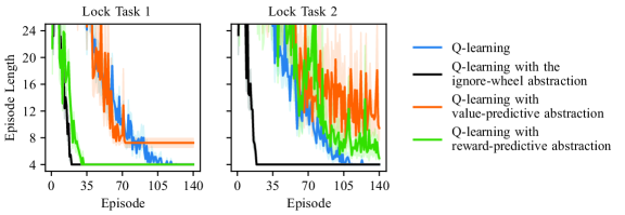
Refer to caption
(a) Combination Lock Tasks
Refer to caption
(b) Performance of Each Model at Transfer
Figure 9: Combination Lock Transfer Experiment. 9(a): In the combination lock tasks, the agent decides between three different actions to rotate each dial by one digit. Each dial has five sides labelled with the digits zero through four. The dark gray dial is “broken” and spins at random at every time step. In the training task, any combination setting the left and middle dial to four are rewarding. In Test Lock 1, setting the left dial to two and the middle dial to three is rewarding and simulations were started by setting the left dial to two and the middle dial to four. In Test Lock 2, setting the left dial to two and the right dial to three is rewarding and simulations were started by setting the left dial to two and the right dial to four. 9(b): Each panel plots the episode length of the Q-learning algorithm on Lock Task 1 and Lock Task 2 averaged over 20 repeats. Note that Q-learning with the ignore-wheel abstraction uses a different abstraction in Test Lock 1 and Test Lock 2. In Test Lock 1, the ignore-wheel abstraction ignores the right dial. In Test Lock 2, the ignore-wheel abstraction ignores the middle dial. Please refer to Appendix C for a detailed description of the experiment implementation.

To determine if a reward- or value-predictive state representation can be re-used to accelerate learning in a previously unseen task, we compute a two-state representations of each type for the Training Lock MDP. To assess if each state abstraction can be re-used, they are both tested by compressing the state space of a Q-learning agent (Watkins and Dayan, 1992) to learn an optimal policy in Test Lock 1 and Test Lock 2. Any resulting performance changes are then indicative of the state abstraction’s ability to generalize from the Training Lock task to Test Lock 1 and Test Lock 2. If a state representation can generalize information from the training to the test task, then Q-learning with a state abstraction should converge to an optimal policy faster than a Q-learning agent that does not use any state abstraction. To combine the tabular Q-learning algorithm with a state abstraction, we assume in this section that a state abstraction function maps each state to a set of discrete latent states. Furthermore, before updating the Q-learning agent with a transition (s,a,r,s)𝑠𝑎𝑟superscript𝑠(s,a,r,s^{\prime}), this transition is mapped to a latent space transition (ϕ(s),a,r,ϕ(s))italic-ϕ𝑠𝑎superscript𝑟italic-ϕ𝑠(\phi(s),a,r^{\prime},\phi(s)) using the respective state abstraction function ϕitalic-ϕ\phi. Because the latent state space is smaller than the task’s original state space, one would expect that using a state abstraction function results in faster convergence, because any Q-value update is generalized across all states that are mapped to the same latent state.

The reward-predictive state representation is computed using the training task’s transition and reward table with the same procedure used for the column-world task presented in Figure 5. (Please also refer to Appendix C for implementation details.) To obtain a state-representation function mapping states to discrete latent states, the real-valued state representation function ϕreal-valued:𝒮n:subscriptitalic-ϕreal-valued𝒮superscript𝑛\phi_{\text{real-valued}}:\mathcal{S}\to\mathbb{R}^{n} is then further refined by clustering the set of feature vectors {ϕreal-valued(s)|s𝒮}conditional-setsubscriptitalic-ϕreal-valued𝑠𝑠𝒮\{\phi_{\text{real-valued}}(s)|s\in\mathcal{S}\} into discrete clusters using agglomerative clustering. Each cluster then becomes a separate latent state in the resulting latent state space.

The value-predictive state representation is computed by associating two states with the same latent state if the optimal policy has equal Q-values at both states and for each action. This type of state abstraction has been previously introduced by Li et al. (2006) as a Qsuperscript𝑄Q^{*}-irrelevance state abstraction and is predictive of Q-values because each latent state is associated with a different set of Q-values.

Figure 9(b) plots the episode length of four different Q-learning agent configurations. The first configuration (blue curves in Figure 9(b)) forms a baseline and simulates the Q-learning algorithm on both test tasks, without using any state abstraction. The second configuration, called “Q-learning with ignore dial abstraction” (black curves in Figure 9(b)) simulates the Q-learning algorithm with a manually coded state abstraction that ignores the right dial in Test Lock 1 and the middle dial in Test Lock 2. Because this state abstraction compresses the 125 task states into 25 latent states by removing the digit from the state triplet not relevant for maximizing reward, this variation converges significantly faster than the baseline algorithm. The third variation, called “Q-learning with value-predictive abstraction” (orange curves in Figure 9(b)) simulates Q-learning with the value-predictive state abstraction. In both Test Lock 1 and Test Lock 2, this variation converges more slowly than using Q-learning without any state abstraction. As discussed in Section 5.2, a value-predictive state abstraction is constructed using the Q-values of the policy that is optimal in the Training Lock. Because each combination lock MDP has a different optimal policy, a value-predictive state abstraction cannot be transferred across any of the two tasks. Consequently, the “Q-learning with a value-predictive abstraction” agent does not converge more quickly than the baseline agent. In these simulations, the Q-learning algorithm is not capable of finding an optimal policy, as outlined previously in Figure 7. The green curves in Figure 9(b) plot the average episode length when Q-learning is combined with a reward-predictive state abstraction. In Lock Task 1, this agent converges almost as fast as the agent using the manually coded state abstraction (black curve, left panel). Only the position of the left and middle dials are relevant for predicting reward sequences r1,,rtsubscript𝑟1subscript𝑟𝑡r_{1},...,r_{t} that are generated by following an arbitrary action sequence a1,,atsubscript𝑎1subscript𝑎𝑡a_{1},...,a_{t} from an arbitrary start state s𝑠s in the Training Lock MDP and in the Test Lock 1 MDP. Consequently, a reward-predictive state abstraction can compress the 125 task states into 25 different latent states by ignoring the right dial, resulting in a significant performance improvement in Test Lock 1. Note that LSFMs only approximate reward-predictive state representations resulting in slightly slower convergence in comparison to the black curve in the left panel of Figure 9(b).

This behaviour changes in Test Lock 2, because in Test Lock 2 a different dial moves at random, changing how the state space should be compressed. Because the right dial is relevant for predicting expected reward sequences in Test Lock 2, the reward-predictive state representation learned in the Training Lock task is no longer reward-predictive in Test Lock 2 and cannot be re-used without modifications. Consequently, the “Q-learning with reward-predictive abstraction” agent exhibits worse performance (Figure 9(b), right panel, green curve) than using Q-learning without any state abstraction (Figure 9(b), right panel, blue curve).

The results presented in Figure 9 demonstrate that reward-predictive state representations encode which state information is relevant for predicting reward sequences and maximizing reward in a task. Because reward-predictive state representations only model this aspect of an MDP, this type of state representation generalizes across tasks that preserve these state equivalences but differ in their transitions and rewards otherwise. In contrast, value-predictive state representations “overfit” to a specific MDP and the MDP’s optimal policy, resulting in negative transfer and possibly prohibiting an agent from finding an optimal policy at transfer.

6 Discussion

LAM(Sutton et al., 2008)s,a𝑠𝑎s,aϕssubscriptbold-italic-ϕ𝑠\boldsymbol{\phi}_{s}𝔼p[ϕ|s,a]subscript𝔼𝑝delimited-[]conditionalsuperscriptbold-italic-ϕ𝑠𝑎\mathbb{E}_{p}[\boldsymbol{\phi}^{\prime}|s,a]r(s,a)𝑟𝑠𝑎r(s,a)𝔼[r1,r2,|s,a1,a2,]\mathbb{E}\left[r_{1},r_{2},...\middle|s,a_{1},a_{2},...\right]ϕitalic-ϕ\phi𝑴asubscript𝑴𝑎\boldsymbol{M}_{a}𝒘asubscript𝒘𝑎\boldsymbol{w}_{a}LSFM s,a𝑠𝑎s,aϕssubscriptbold-italic-ϕ𝑠\boldsymbol{\phi}_{s}𝝍π(s,a)superscript𝝍𝜋𝑠𝑎\boldsymbol{\psi}^{\pi}(s,a)r(s,a)𝑟𝑠𝑎r(s,a)𝔼[r1,r2,|s,a1,a2,]\mathbb{E}\left[r_{1},r_{2},...\middle|s,a_{1},a_{2},...\right]ϕitalic-ϕ\phi𝑭asubscript𝑭𝑎\boldsymbol{F}_{a}𝒘asubscript𝒘𝑎\boldsymbol{w}_{a}SF(Barreto et al., 2017a)s,a𝑠𝑎s,a𝝃s,asubscript𝝃𝑠𝑎\boldsymbol{\xi}_{s,a}𝝍π(s,a)superscript𝝍𝜋𝑠𝑎\boldsymbol{\psi}^{\pi}(s,a)r(s,a)𝑟𝑠𝑎r(s,a)Qπsuperscript𝑄𝜋Q^{\pi}ξ𝜉\xiψ𝜓\psi𝒘𝒘\boldsymbol{w}𝒘𝒘\boldsymbol{w}Fitted Q-Iteration(Riedmiller, 2005)s,a𝑠𝑎s,aϕssubscriptbold-italic-ϕ𝑠\boldsymbol{\phi}_{s}Qπsuperscript𝑄𝜋Q^{\pi}ϕitalic-ϕ\phi𝒒asubscript𝒒𝑎\boldsymbol{q}_{a}Reward-Predictive Models (model-based RL)Value-Predictive Models (model-free RL)Temporal Difference Learning: Representation Map (arbitrary function): Prediction (linear if annotated with a matrix or vector)
Figure 10: Comparison of Presented State-Representation Models.

This article presents a study of how successor features combine aspects of model-free and model-based RL. Connections are drawn by analyzing which properties different latent state spaces are predictive of. The schematic in Figure 10 illustrates the differences between the presented models. By introducing LSFMs, SFs are tied to learning state representations that are predictive of future expected reward outcomes. This model ties successor features to model-based reinforcement learning, because an agent that has learned an LSFM can predict expected future reward outcomes for any arbitrary action sequence. While this connection to model-based RL has been previously hypothesized (Russek et al., 2017; Momennejad et al., 2017), LSFMs formalize this connection. Because SFs obey a fixed-point equation similar to the Bellman fixed-point equation, SFs can also be linked to temporal-difference learning. Similar to LAMs, LSFMs are a “strict” model-based architecture and are distinct from model-based and model-free hybrid architectures that iteratively search for an optimal policy and adjust their internal representation (Oh et al., 2017; Weber et al., 2017; François-Lavet et al., 2019; Gelada et al., 2019). LSFMs only evaluate SFs for a fixed target policy that selects actions uniformly at random. The learned model can then be used to predict the value function of any arbitrary policy, including the optimal policy. In contrast to model-based and model-free hybrid architectures, the learned state representation does not have to be adopted to predict an optimal policy and generalizes across all latent policies. How to learn neural networks mapping inputs to latent feature spaces that are predictive of future reward outcomes is beyond the scope of this article and is left for future work.

Similar to reward-predictive state representations, the Predictron architecture (Silver et al., 2017) and the MuZero algorithm (Schrittwieser et al., 2019) use or construct a state representation to predict reward sequences. In contrast to reward-predictive state representations, these other architectures predict reward sequences for k𝑘k time steps and then use the value function for one (or multiple) policies to predict the return obtained after k𝑘k time steps. This distinction is key in learning reward-predictive state representations with LSFMs, which do not include a value prediction module, because if a state representation is designed to predict the value function of a policy, then the resulting state representation would be (to some extent) value predictive. As outlined in Section 5, this change would compromise the resulting state abstraction’s ability to generalize across different transition and reward functions.

In contrast to the SF framework introduced by Barreto et al. (2017a), the connection between LSFMs and model-based RL is possible because the same state representation ϕitalic-ϕ\phi is used to predict its own SF (Figure 10 center column). While the deep learning models presented by Kulkarni et al. (2016) and Zhang et al. (2017) also use one state representation to predict SFs and one-step rewards, these models are also constrained to predict image frames. LSFMs do not use the state representation to reconstruct actual states. Instead, the state space is explicitly compressed, allowing the agent to generalize across distinct states.

Table 1 summarizes different properties of the presented state representations. Bisimulation relations (Givan et al., 2003) preserve most structure of the original MDP and latent transition probabilities match with transition probabilities in the original MDP (Section 4.1). Reward-predictive state representations do not preserve the transition probabilities of the original task (Figure 4) but construct a latent state space that is predictive of expected future reward outcomes. These two representations generalize across all abstract policies, because they can predict reward outcomes for arbitrary action sequences. Successor features are equivalent to value-predictive state representations, which construct a latent state space that is predictive of a policy’s value function (Section 5). Because the value function can be factored into SFs and a reward model (Equation (37)), SFs are robust to variations in reward functions. Reward-predictive state representations remove previous limitations of SFs and generalize across variations in transition functions. This property stands in contrast to previous work on SFs, which demostrate robustness against changes in the reward function only (Barreto et al., 2017a, 2018; Kulkarni et al., 2016; Zhang et al., 2017; Stachenfeld et al., 2017; Momennejad et al., 2017; Russek et al., 2017). In all cases, including reward-predictive state representations, the learned models can only generalize to changes that approximately preserve the latent state space structure. For example, in Figure 8 positive transfer is possible because both tasks are grid worlds and only the locations of rewards and barriers is changed. If the same representation is used on a completely different randomly generated finite MDP, then positive transfer may not be possible because both tasks do not have a latent state structure in common.

Model Predicts Trained Policy Generalizes to Variations in Rewards Generalizes to Variations in Transitions Generalizes Across All Policies Predicts Transition Probabilities
Bisimulation          (Givan et al., 2003) yes yes yes yes yes
Reward-Predictive (LSFM or LAM) yes yes yes yes no
Successor Features                     (Barreto et al., 2017a) yes yes no no no
Value-Predictive (Fitted Q-iteration) yes no no no no
Table 1: Summary of Generalization Properties of Presented State Representations

In comparison to previous work on state abstractions (Even-Dar and Mansour, 2003; Li et al., 2006; Abel et al., 2016, 2018, 2019), this article does not consider state representations that compress the state space as much as possible. Instead, the degree of compression is set through the hyper-parameter that controls the dimension of the constructed latent state space. The presented experiments demonstrate that these state representations compress the state space and implicitly convey information useful for transfer. This formulation of state representations connects ideas from state abstractions to models that analyze linear basis functions (Parr et al., 2008; Sutton, 1996; Konidaris et al., 2011) or learn linear representations of the transition and reward functions (Song et al., 2016). Recently, Ruan et al. (2015) presented algorithms to cluster approximately bisimilar states. Their method relies on bisimulation metrics (Ferns et al., 2004), which use the Wasserstein metric to assess if two state transitions have the same distribution over next state clusters. In contrast to their approach, we phrase learning reward-predictive state representations as an energy-minimization problem and remove the requirement of computing the Wasserstein metric.

The presented experiments learn state representations by generating a transition data set covering all states of an MDP. Complete coverage is obtained on the grid world tasks by generating a large enough transition data set. Because this article focuses on drawing connections between different models of generalization across states, combining the presented algorithms with efficient exploration algorithms (Jin et al., 2018) or obtaining sample complexity or regret bounds similar to prior work (Jaksch et al., 2010; Azar et al., 2017; Osband et al., 2013) is left to future studies.

7 Conclusion

This article presents an analysis of which latent representations an intelligent agent can construct to support different predictions, leading to new connections between model-based and model-free RL. By introducing LSFMs, the presented analysis links learning successor features to model-based RL and demonstrates that the learned reward-predictive state representations are suitable for transfer across variations in transitions and rewards. The presented results outline how different models of generalization are related to another and proposes a model for phrasing model-based learning as a representation-learning problem. These results motivate the design and further investigation of new approximate model-based RL algorithms that learn state representations instead of one-step reward and transition models.


Acknowledgments

We would like to thank Prof. Michael J. Frank for many insightful discussions that benefited the development of the presented work. This project was supported in part by the ONR MURI PERISCOPE project and in part by the NIH T32 Training Grant on Interactionist Cognitive Neuroscience.

A Proofs of Theoretical Results

This section lists formal proofs for all presented theorems and propositions.

A.1 Bisimulation Theorems

For an equivalence relation similar-to\sim defined on a set 𝒮𝒮\mathcal{S}, the set of all partition is denoted with 𝒮/\mathcal{S}/\sim. Each partition [s]𝒮/[s]\in\mathcal{S}/\sim is a subset of 𝒮𝒮\mathcal{S} and s[s]𝑠delimited-[]𝑠s\in[s].

Definition 4 (Bisimilarity (Ferns et al., 2011)).

For an MDP M=𝒮,𝒜,p,r,γ𝑀𝒮𝒜𝑝𝑟𝛾M=\langle\mathcal{S},\mathcal{A},p,r,\gamma\rangle where 𝒮,Σ,p𝒮Σ𝑝\langle\mathcal{S},\Sigma,p\rangle is a measurable space with σ𝜎\sigma-algebra ΣΣ\Sigma and p𝑝p is a Markov kernel labelled for each action a𝒜𝑎𝒜a\in\mathcal{A}. Consider an equivalence relation bsubscriptsimilar-to𝑏\sim_{b} on the state space 𝒮𝒮\mathcal{S} such that each state partition [s]delimited-[]superscript𝑠[s^{\prime}] also lies in the σ𝜎\sigma-algebra and [s]𝒮/b\forall[s^{\prime}]\in\mathcal{S}/\sim_{b}, [s]Σdelimited-[]superscript𝑠Σ[s^{\prime}]\in\Sigma. The equivalence relation bsubscriptsimilar-to𝑏\sim_{b} is a bisimulation if

sbs~iffsubscriptsimilar-to𝑏𝑠~𝑠absent\displaystyle s\sim_{b}\tilde{s}\iff a𝒜,𝔼p[r(s,a,s)|s,a]=𝔼p[r(s~,a,s)|s~,a]\displaystyle\forall a\in\mathcal{A},~{}\mathbb{E}_{p}\left[r(s,a,s^{\prime})\middle|s,a\right]=\mathbb{E}_{p}\left[r(\tilde{s},a,s^{\prime})\middle|\tilde{s},a\right] (48)
and[s]𝒮/b,p([s]|s,a)=p([s]|s~,a).\displaystyle\text{and}~{}\forall[s^{\prime}]\in\mathcal{S}/\sim_{b},~{}p([s^{\prime}]|s,a)=p([s^{\prime}]|\tilde{s},a). (49)

Using this definition, Theorem 1 can be proven.

Proof of Theorem 1.

Consider any two states s𝑠s and s~~𝑠\tilde{s} such that ϕs=ϕs~subscriptbold-italic-ϕ𝑠subscriptbold-italic-ϕ~𝑠\boldsymbol{\phi}_{s}=\boldsymbol{\phi}_{\tilde{s}}. For both s𝑠s and s~~𝑠\tilde{s} we have

𝔼p[r(s,a,s)|s,a]=ϕs𝒘a=ϕs~𝒘a=𝔼p[r(s~,a,s)|s~,a],\mathbb{E}_{p}\left[r(s,a,s^{\prime})\middle|s,a\right]=\boldsymbol{\phi}_{s}^{\top}\boldsymbol{w}_{a}=\boldsymbol{\phi}_{\tilde{s}}^{\top}\boldsymbol{w}_{a}=\mathbb{E}_{p}\left[r(\tilde{s},a,s^{\prime})\middle|\tilde{s},a\right], (50)

and the bisimulation reward condition in Equation (48) holds. To show that also the bisimulation transition condition in Equation (49) holds, observe that

ϕssuperscriptsubscriptbold-italic-ϕ𝑠top\displaystyle\boldsymbol{\phi}_{s}^{\top} =ϕs~absentsuperscriptsubscriptbold-italic-ϕ~𝑠top\displaystyle=\boldsymbol{\phi}_{\tilde{s}}^{\top} iff\displaystyle\iff (51)
ϕs𝑴asuperscriptsubscriptbold-italic-ϕ𝑠topsubscript𝑴𝑎\displaystyle\boldsymbol{\phi}_{s}^{\top}\boldsymbol{M}_{a} =ϕs~𝑴aabsentsuperscriptsubscriptbold-italic-ϕ~𝑠topsubscript𝑴𝑎\displaystyle=\boldsymbol{\phi}_{\tilde{s}}^{\top}\boldsymbol{M}_{a} iff\displaystyle\iff (52)
𝔼p[ϕs|s,a]\displaystyle\mathbb{E}_{p}\left[\boldsymbol{\phi}_{s^{\prime}}\middle|s,a\right] =𝔼p[ϕs|s~,a]\displaystyle=\mathbb{E}_{p}\left[\boldsymbol{\phi}_{s^{\prime}}\middle|\tilde{s},a\right] iff\displaystyle\iff (53)
i=1np(s,a,[si])𝒆isuperscriptsubscript𝑖1𝑛𝑝𝑠𝑎delimited-[]subscript𝑠𝑖subscript𝒆𝑖\displaystyle\sum_{i=1}^{n}p(s,a,[s_{i}])\boldsymbol{e}_{i} =i=1np(s~,a,[si])𝒆i,absentsuperscriptsubscript𝑖1𝑛𝑝~𝑠𝑎delimited-[]subscript𝑠𝑖subscript𝒆𝑖\displaystyle=\sum_{i=1}^{n}p(\tilde{s},a,[s_{i}])\boldsymbol{e}_{i}, (54)

where [si]𝒮delimited-[]subscript𝑠𝑖𝒮[s_{i}]\subset\mathcal{S} are all states that are mapped to the one-hot feature vector 𝒆isubscript𝒆𝑖\boldsymbol{e}_{i}. Each side of the identity (54) computes an expectation over one-hot bit vectors and thus the i𝑖ith entry of i=1np(s,a,[si])𝒆isuperscriptsubscript𝑖1𝑛𝑝𝑠𝑎delimited-[]subscript𝑠𝑖subscript𝒆𝑖\sum_{i=1}^{n}p(s,a,[s_{i}])\boldsymbol{e}_{i} contains the probability value p(s,a,[si])𝑝𝑠𝑎delimited-[]subscript𝑠𝑖p(s,a,[s_{i}]). Hence both s𝑠s and s~~𝑠\tilde{s} have equal probabilities of transitioning into each state partition that is associated with 𝒆isubscript𝒆𝑖\boldsymbol{e}_{i}. Define an equivalence relation ϕsubscriptsimilar-toitalic-ϕ\sim_{\phi} such that

s,s~𝒮,ϕs=ϕs~sϕs~.\forall s,\tilde{s}\in\mathcal{S},~{}\boldsymbol{\phi}_{s}=\boldsymbol{\phi}_{\tilde{s}}\iff s\sim_{\phi}\tilde{s}. (55)

Because all feature vectors ϕssubscriptbold-italic-ϕ𝑠\boldsymbol{\phi}_{s} are one-hot bit vectors, there are at most n𝑛n partitions and the set of all state partitions has size |𝒮/ϕ|=n|\mathcal{S}/\sim_{\phi}|=n. Combining these observations, Equation (54) can be rewritten as

[s]𝒮/ϕ,p([s]|s,a)=p([s]|s~,a).\forall[s^{\prime}]\in\mathcal{S}/\sim_{\phi},~{}p([s^{\prime}]|s,a)=p([s^{\prime}]|\tilde{s},a). (56)

By lines (50) and (56), the equivalence relation ϕsubscriptsimilar-toitalic-ϕ\sim_{\phi} is a bisimulation relation and if ϕs=ϕs~subscriptbold-italic-ϕ𝑠subscriptbold-italic-ϕ~𝑠\boldsymbol{\phi}_{s}=\boldsymbol{\phi}_{\tilde{s}} then both s𝑠s and s~~𝑠\tilde{s} are bisimilar. ∎

Lemma 2.

Assume an MDP, state representation ϕ:𝒮{𝐞1,,𝐞n}:italic-ϕ𝒮subscript𝐞1subscript𝐞𝑛\phi:\mathcal{S}\to\{\boldsymbol{e}_{1},...,\boldsymbol{e}_{n}\}, LSFM {𝐅a,𝐰a}a𝒜subscriptsubscript𝐅𝑎subscript𝐰𝑎𝑎𝒜\{\boldsymbol{F}_{a},\boldsymbol{w}_{a}\}_{a\in\mathcal{A}}, and arbitrary policy πΠϕ𝜋subscriptΠitalic-ϕ\pi\in\Pi_{\phi}. Let 𝐅πsuperscript𝐅𝜋\boldsymbol{F}^{\pi} be an n×n𝑛𝑛n\times n real valued matrix with each row 𝐅π(i)=𝔼π[𝐞i𝐅a|s]\boldsymbol{F}^{\pi}(i)=\mathbb{E}_{\pi}\left[\boldsymbol{e}_{i}^{\top}\boldsymbol{F}_{a}\middle|s\right], then

𝔼π[ϕs𝑭a|s]=𝒆i𝑭π,\mathbb{E}_{\pi}\left[\boldsymbol{\phi}_{s}^{\top}\boldsymbol{F}_{a}\middle|s\right]=\boldsymbol{e}_{i}^{\top}\boldsymbol{F}^{\pi}, (57)

where ϕs=𝐞isubscriptbold-ϕ𝑠subscript𝐞𝑖\boldsymbol{\phi}_{s}=\boldsymbol{e}_{i} for some i𝑖i. For a LAM {𝐌a,𝐰a}a𝒜subscriptsubscript𝐌𝑎subscript𝐰𝑎𝑎𝒜\{\boldsymbol{M}_{a},\boldsymbol{w}_{a}\}_{a\in\mathcal{A}}, let 𝐌πsuperscript𝐌𝜋\boldsymbol{M}^{\pi} be a n×n𝑛𝑛n\times n real-valued matrix with each row 𝐌π(i)=𝔼π[𝐞i𝐌a|s]\boldsymbol{M}^{\pi}(i)=\mathbb{E}_{\pi}\left[\boldsymbol{e}_{i}^{\top}\boldsymbol{M}_{a}\middle|s\right], then

𝔼π[ϕs𝑴a|s]=𝒆i𝑴π.\mathbb{E}_{\pi}\left[\boldsymbol{\phi}_{s}^{\top}\boldsymbol{M}_{a}\middle|s\right]=\boldsymbol{e}_{i}^{\top}\boldsymbol{M}^{\pi}. (58)
Proof of Lemma 2.

The first identities in (57) and (58) hold because ϕs=𝒆isubscriptbold-italic-ϕ𝑠subscript𝒆𝑖\boldsymbol{\phi}_{s}=\boldsymbol{e}_{i} for some i𝑖i. Then,

𝔼π[ϕs𝑭a|s]=aπ(s,a)ϕs𝑭a=aπ(s,a)𝒆i𝑭a=𝔼π[𝒆i𝑭a|s]=𝑭π(i)=𝒆i𝑭π\mathbb{E}_{\pi}\left[\boldsymbol{\phi}_{s}^{\top}\boldsymbol{F}_{a}\middle|s\right]=\sum_{a}\pi(s,a)\boldsymbol{\phi}_{s}\boldsymbol{F}_{a}=\sum_{a}\pi(s,a)\boldsymbol{e}_{i}^{\top}\boldsymbol{F}_{a}=\mathbb{E}_{\pi}\left[\boldsymbol{e}_{i}^{\top}\boldsymbol{F}_{a}\middle|s\right]=\boldsymbol{F}^{\pi}(i)=\boldsymbol{e}_{i}^{\top}\boldsymbol{F}^{\pi}

and

𝔼π[ϕs𝑴a|s]=aπ(s,a)ϕs𝑴a=aπ(s,a)𝒆i𝑴a=𝔼π[𝒆i𝑴a|s]=𝑴π(i)=𝒆i𝑴π.\mathbb{E}_{\pi}\left[\boldsymbol{\phi}_{s}^{\top}\boldsymbol{M}_{a}\middle|s\right]=\sum_{a}\pi(s,a)\boldsymbol{\phi}_{s}\boldsymbol{M}_{a}=\sum_{a}\pi(s,a)\boldsymbol{e}_{i}^{\top}\boldsymbol{M}_{a}=\mathbb{E}_{\pi}\left[\boldsymbol{e}_{i}^{\top}\boldsymbol{M}_{a}\middle|s\right]=\boldsymbol{M}^{\pi}(i)=\boldsymbol{e}_{i}^{\top}\boldsymbol{M}^{\pi}.

Definition 5 (Weighting Function).

For an MDP M=𝒮,𝒜,p,r,γ𝑀𝒮𝒜𝑝𝑟𝛾M=\langle\mathcal{S},\mathcal{A},p,r,\gamma\rangle, let similar-to\sim be an equivalence relation on the state space 𝒮𝒮\mathcal{S}, creating a set of state partitions 𝒮/\mathcal{S}/\sim. Assume that each state partition [s]delimited-[]𝑠[s] is a measurable space [s],Σ[s],ω[s]delimited-[]𝑠subscriptΣdelimited-[]𝑠subscript𝜔delimited-[]𝑠\langle[s],\Sigma_{[s]},\omega_{[s]}\rangle, where ω[s]subscript𝜔delimited-[]𝑠\omega_{[s]} is a probability measure indexed by each partition [s]delimited-[]𝑠[s] with σ𝜎\sigma-algebra Σ[s]subscriptΣdelimited-[]𝑠\Sigma_{[s]}. The function ω𝜔\omega is called the weighting function.

Lemma 3.

Assume an MDP, state representation ϕ:𝒮{𝐞1,,𝐞n}:italic-ϕ𝒮subscript𝐞1subscript𝐞𝑛\phi:\mathcal{S}\to\{\boldsymbol{e}_{1},...,\boldsymbol{e}_{n}\}, LSFM {𝐅a,𝐰a}a𝒜subscriptsubscript𝐅𝑎subscript𝐰𝑎𝑎𝒜\{\boldsymbol{F}_{a},\boldsymbol{w}_{a}\}_{a\in\mathcal{A}}, and arbitrary abstract policy πΠϕ𝜋subscriptΠitalic-ϕ\pi\in\Pi_{\phi}. Then,

s,aϕs𝑭a=ϕs+γ𝔼p,π[ϕs𝑭a|s,a]s,a,𝑴asuch that𝑭a=𝑰+γ𝑴a𝑭π,\forall s,\forall a~{}\boldsymbol{\phi}_{s}^{\top}\boldsymbol{F}_{a}=\boldsymbol{\phi}_{s}^{\top}+\gamma\mathbb{E}_{p,\pi}\left[\boldsymbol{\phi}_{s^{\prime}}\boldsymbol{F}_{a^{\prime}}\middle|s,a\right]\implies\forall s,\forall a,\exists\boldsymbol{M}_{a}~{}\text{such that}~{}\boldsymbol{F}_{a}=\boldsymbol{I}+\gamma\boldsymbol{M}_{a}\boldsymbol{F}^{\pi}, (59)

where the matrix 𝐅πsuperscript𝐅𝜋\boldsymbol{F}^{\pi} is constructed as described in Lemma 2.

Proof of Lemma 3.

Consider an equivalence relation ϕsubscriptsimilar-toitalic-ϕ\sim_{\phi} that is constructed using the state representation ϕitalic-ϕ\phi and

s,s~𝒮,ϕs=ϕs~sϕs~.\forall s,\tilde{s}\in\mathcal{S},~{}\boldsymbol{\phi}_{s}=\boldsymbol{\phi}_{\tilde{s}}\iff s\sim_{\phi}\tilde{s}. (60)

The weighting function ω𝜔\omega models a probability distribution of density function of visiting a state s𝑠s that belongs to a state partition [s]𝒮/ϕ[s]\in\mathcal{S}/\sim_{\phi}. Because all states s[s]𝑠delimited-[]𝑠s\in[s] are mapped to the same feature vector ϕssubscriptbold-italic-ϕ𝑠\boldsymbol{\phi}_{s}, we have that

𝔼ω[s][ϕs]=ϕs.subscript𝔼subscript𝜔delimited-[]𝑠delimited-[]subscriptbold-italic-ϕ𝑠subscriptbold-italic-ϕ𝑠\mathbb{E}_{\omega_{[s]}}\left[\boldsymbol{\phi}_{s}\right]=\boldsymbol{\phi}_{s}. (61)

The stochastic matrix 𝑴asubscript𝑴𝑎\boldsymbol{M}_{a} is defined for every action a𝑎a as

𝑴a(i,j)=𝔼ω[s][Pr{s𝑎𝒆j}]withϕs=𝒆i,subscript𝑴𝑎𝑖𝑗subscript𝔼subscript𝜔delimited-[]𝑠delimited-[]Pr𝑠𝑎subscript𝒆𝑗withsubscriptbold-italic-ϕ𝑠subscript𝒆𝑖\boldsymbol{M}_{a}(i,j)=\mathbb{E}_{\omega_{[s]}}\left[\text{Pr}\left\{s\overset{a}{\to}\boldsymbol{e}_{j}\right\}\right]~{}\text{with}~{}\boldsymbol{\phi}_{s}=\boldsymbol{e}_{i}, (62)

where Pr{s𝑎𝒆j}Pr𝑠𝑎subscript𝒆𝑗\text{Pr}\left\{s\overset{a}{\to}\boldsymbol{e}_{j}\right\} is the probability of transitioning into the state partition associated with the latent state 𝒆jsubscript𝒆𝑗\boldsymbol{e}_{j} and

Pr{s𝑎𝒆j}=p(s,a,[si])such thats[si],ϕ(s)=𝒆j.formulae-sequencePr𝑠𝑎subscript𝒆𝑗𝑝𝑠𝑎delimited-[]subscript𝑠𝑖such thatfor-all𝑠delimited-[]subscript𝑠𝑖italic-ϕ𝑠subscript𝒆𝑗\text{Pr}\left\{s\overset{a}{\to}\boldsymbol{e}_{j}\right\}=p(s,a,[s_{i}])~{}\text{such that}~{}\forall s\in[s_{i}],\phi(s)=\boldsymbol{e}_{j}. (63)

The identity in Equation (59) can be re-written as follows:

ϕs𝑭asuperscriptsubscriptbold-italic-ϕ𝑠topsubscript𝑭𝑎\displaystyle\boldsymbol{\phi}_{s}^{\top}\boldsymbol{F}_{a} =ϕs+γ𝔼p,π[ϕs𝑭a|s,a]\displaystyle=\boldsymbol{\phi}_{s}^{\top}+\gamma\mathbb{E}_{p,\pi}\left[\boldsymbol{\phi}_{s^{\prime}}\boldsymbol{F}_{a^{\prime}}\middle|s,a\right] iff\displaystyle\iff
ϕs𝑭asuperscriptsubscriptbold-italic-ϕ𝑠topsubscript𝑭𝑎\displaystyle\boldsymbol{\phi}_{s}^{\top}\boldsymbol{F}_{a} =ϕs+γ𝔼p[ϕs|s,a]𝑭π\displaystyle=\boldsymbol{\phi}_{s}^{\top}+\gamma\mathbb{E}_{p}\left[\boldsymbol{\phi}_{s^{\prime}}\middle|s,a\right]\boldsymbol{F}^{\pi} iff\displaystyle\iff (by Lemma 2)by Lemma 2\displaystyle(\text{by~{}Lemma~{}\ref{lem:pi-cond-mat}})
𝔼ω[s][ϕs𝑭a]subscript𝔼subscript𝜔delimited-[]𝑠delimited-[]superscriptsubscriptbold-italic-ϕ𝑠topsubscript𝑭𝑎\displaystyle\mathbb{E}_{\omega_{[s]}}\left[\boldsymbol{\phi}_{s}^{\top}\boldsymbol{F}_{a}\right] =𝔼ω[s][(ϕs+γ𝔼p[ϕs|s,a])𝑭π]\displaystyle=\mathbb{E}_{\omega_{[s]}}\left[\left(\boldsymbol{\phi}_{s}^{\top}+\gamma\mathbb{E}_{p}\left[\boldsymbol{\phi}_{s^{\prime}}\middle|s,a\right]\right)\boldsymbol{F}^{\pi}\right] iff\displaystyle\iff
ϕs𝑭asuperscriptsubscriptbold-italic-ϕ𝑠topsubscript𝑭𝑎\displaystyle\boldsymbol{\phi}_{s}^{\top}\boldsymbol{F}_{a} =ϕs+γ𝔼ω[s][𝔼p[ϕs|s,a]]𝑭π\displaystyle=\boldsymbol{\phi}_{s}^{\top}+\gamma\mathbb{E}_{\omega_{[s]}}\left[\mathbb{E}_{p}\left[\boldsymbol{\phi}_{s^{\prime}}\middle|s,a\right]\right]\boldsymbol{F}^{\pi} iff\displaystyle\iff (by (61))by (61)\displaystyle(\text{by~{}\eqref{eq:lem-f-mat-id-1}})
ϕs𝑭asuperscriptsubscriptbold-italic-ϕ𝑠topsubscript𝑭𝑎\displaystyle\boldsymbol{\phi}_{s}^{\top}\boldsymbol{F}_{a} =ϕs+γ𝔼ω[s][j=1nPr{s𝑎𝒆j}𝒆j]𝑭πabsentsuperscriptsubscriptbold-italic-ϕ𝑠top𝛾subscript𝔼subscript𝜔delimited-[]𝑠delimited-[]superscriptsubscript𝑗1𝑛Pr𝑠𝑎subscript𝒆𝑗superscriptsubscript𝒆𝑗topsuperscript𝑭𝜋\displaystyle=\boldsymbol{\phi}_{s}^{\top}+\gamma\mathbb{E}_{\omega_{[s]}}\left[\sum_{j=1}^{n}\text{Pr}\left\{s\overset{a}{\to}\boldsymbol{e}_{j}\right\}\boldsymbol{e}_{j}^{\top}\right]\boldsymbol{F}^{\pi} iff\displaystyle\iff
ϕs𝑭asuperscriptsubscriptbold-italic-ϕ𝑠topsubscript𝑭𝑎\displaystyle\boldsymbol{\phi}_{s}^{\top}\boldsymbol{F}_{a} =ϕs+γ[𝔼ω[s][Pr{s𝑎𝒆1}],,𝔼ω[s][Pr{s𝑎𝒆n}]]n-dimensional row vector, because 𝒆j is one-hot𝑭πabsentsuperscriptsubscriptbold-italic-ϕ𝑠top𝛾subscriptsubscript𝔼subscript𝜔delimited-[]𝑠delimited-[]Pr𝑠𝑎subscript𝒆1subscript𝔼subscript𝜔delimited-[]𝑠delimited-[]Pr𝑠𝑎subscript𝒆𝑛n-dimensional row vector, because 𝒆j is one-hotsuperscript𝑭𝜋\displaystyle=\boldsymbol{\phi}_{s}^{\top}+\gamma\underbrace{\left[\mathbb{E}_{\omega_{[s]}}\left[\text{Pr}\left\{s\overset{a}{\to}\boldsymbol{e}_{1}\right\}\right],...,\mathbb{E}_{\omega_{[s]}}\left[\text{Pr}\left\{s\overset{a}{\to}\boldsymbol{e}_{n}\right\}\right]\right]}_{\text{$n$-dimensional row vector, because $\boldsymbol{e}_{j}$ is one-hot}}\boldsymbol{F}^{\pi} iff\displaystyle\iff
ϕs𝑭asuperscriptsubscriptbold-italic-ϕ𝑠topsubscript𝑭𝑎\displaystyle\boldsymbol{\phi}_{s}^{\top}\boldsymbol{F}_{a} =ϕs+γ[𝑴a(i,1),,𝑴a(i,n)]𝑭πabsentsuperscriptsubscriptbold-italic-ϕ𝑠top𝛾subscript𝑴𝑎𝑖1subscript𝑴𝑎𝑖𝑛superscript𝑭𝜋\displaystyle=\boldsymbol{\phi}_{s}^{\top}+\gamma\left[\boldsymbol{M}_{a}(i,1),...,\boldsymbol{M}_{a}(i,n)\right]\boldsymbol{F}^{\pi} iff\displaystyle\iff (by (62))by (62)\displaystyle(\text{by~{}\eqref{eq:lem-f-mat-id-2}})
ϕs𝑭asuperscriptsubscriptbold-italic-ϕ𝑠topsubscript𝑭𝑎\displaystyle\boldsymbol{\phi}_{s}^{\top}\boldsymbol{F}_{a} =ϕs+γϕs𝑴a𝑭πabsentsuperscriptsubscriptbold-italic-ϕ𝑠top𝛾superscriptsubscriptbold-italic-ϕ𝑠topsubscript𝑴𝑎superscript𝑭𝜋\displaystyle=\boldsymbol{\phi}_{s}^{\top}+\gamma\boldsymbol{\phi}_{s}^{\top}\boldsymbol{M}_{a}\boldsymbol{F}^{\pi} iff\displaystyle\iff (by ϕs=𝒆i)by ϕs=𝒆i\displaystyle(\text{by $\boldsymbol{\phi}_{s}=\boldsymbol{e}_{i}$})
ϕs𝑭asuperscriptsubscriptbold-italic-ϕ𝑠topsubscript𝑭𝑎\displaystyle\boldsymbol{\phi}_{s}^{\top}\boldsymbol{F}_{a} =ϕs(𝑰+γ𝑴a𝑭π)absentsuperscriptsubscriptbold-italic-ϕ𝑠top𝑰𝛾subscript𝑴𝑎superscript𝑭𝜋\displaystyle=\boldsymbol{\phi}_{s}^{\top}\left(\boldsymbol{I}+\gamma\boldsymbol{M}_{a}\boldsymbol{F}^{\pi}\right) (64)

Equation (64) holds for any arbitrary state s𝑠s and because each state is mapped to a one of the one-hot vectors {𝒆1,,𝒆n}subscript𝒆1subscript𝒆𝑛\{\boldsymbol{e}_{1},...,\boldsymbol{e}_{n}\},

i{1,,n},𝒆i𝑭afor-all𝑖1𝑛superscriptsubscript𝒆𝑖topsubscript𝑭𝑎\displaystyle\forall i\in\{1,...,n\},~{}\boldsymbol{e}_{i}^{\top}\boldsymbol{F}_{a} =𝒆i(𝑰+γ𝑴a𝑭π)absentsuperscriptsubscript𝒆𝑖top𝑰𝛾subscript𝑴𝑎superscript𝑭𝜋\displaystyle=\boldsymbol{e}_{i}^{\top}\left(\boldsymbol{I}+\gamma\boldsymbol{M}_{a}\boldsymbol{F}^{\pi}\right) iff\displaystyle\iff
𝑭asubscript𝑭𝑎\displaystyle\boldsymbol{F}_{a} =𝑰+γ𝑴a𝑭π.absent𝑰𝛾subscript𝑴𝑎superscript𝑭𝜋\displaystyle=\boldsymbol{I}+\gamma\boldsymbol{M}_{a}\boldsymbol{F}^{\pi}.

Lemma 4.

Consider a state representation ϕ:𝒮{𝐞1,,𝐞n}:italic-ϕ𝒮subscript𝐞1subscript𝐞𝑛\phi:\mathcal{S}\to\{\boldsymbol{e}_{1},...,\boldsymbol{e}_{n}\}, an arbitrary abstract policy πΠϕ𝜋subscriptΠitalic-ϕ\pi\in\Pi_{\phi}, an LSFM {𝐅a,𝐰a}a𝒜subscriptsubscript𝐅𝑎subscript𝐰𝑎𝑎𝒜\{\boldsymbol{F}_{a},\boldsymbol{w}_{a}\}_{a\in\mathcal{A}} and LAM {𝐌a,𝐰a}a𝒜subscriptsubscript𝐌𝑎subscript𝐰𝑎𝑎𝒜\{\boldsymbol{M}_{a},\boldsymbol{w}_{a}\}_{a\in\mathcal{A}} where each transition matrix 𝐌asubscript𝐌𝑎\boldsymbol{M}_{a} is stochastic. Then,

𝑭a=𝑰+γ𝑴a𝑭π(𝑭π)1and(𝑭π)1=𝑰γ𝑴π,subscript𝑭𝑎𝑰𝛾subscript𝑴𝑎superscript𝑭𝜋superscriptsuperscript𝑭𝜋1andsuperscriptsuperscript𝑭𝜋1𝑰𝛾superscript𝑴𝜋\boldsymbol{F}_{a}=\boldsymbol{I}+\gamma\boldsymbol{M}_{a}\boldsymbol{F}^{\pi}\implies\exists\left(\boldsymbol{F}^{\pi}\right)^{-1}~{}\text{and}~{}\left(\boldsymbol{F}^{\pi}\right)^{-1}=\boldsymbol{I}-\gamma\boldsymbol{M}^{\pi}, (65)

where the matrix 𝐌πsuperscript𝐌𝜋\boldsymbol{M}^{\pi} is constructed as described in Lemma 2.

Proof of Lemma (4).

By Lemma 2, one can write for any arbitrary i𝑖i

𝒆i𝑭πsuperscriptsubscript𝒆𝑖topsuperscript𝑭𝜋\displaystyle\boldsymbol{e}_{i}^{\top}\boldsymbol{F}^{\pi} =𝔼π[𝒆i𝑭a]absentsubscript𝔼𝜋delimited-[]superscriptsubscript𝒆𝑖topsubscript𝑭𝑎\displaystyle=\mathbb{E}_{\pi}\left[\boldsymbol{e}_{i}^{\top}\boldsymbol{F}_{a}\right] iff\displaystyle\iff
𝒆i𝑭πsuperscriptsubscript𝒆𝑖topsuperscript𝑭𝜋\displaystyle\boldsymbol{e}_{i}^{\top}\boldsymbol{F}^{\pi} =𝔼π[𝒆i(𝑰+γ𝑴a𝑭π)]absentsubscript𝔼𝜋delimited-[]superscriptsubscript𝒆𝑖top𝑰𝛾subscript𝑴𝑎superscript𝑭𝜋\displaystyle=\mathbb{E}_{\pi}\left[\boldsymbol{e}_{i}^{\top}(\boldsymbol{I}+\gamma\boldsymbol{M}_{a}\boldsymbol{F}^{\pi})\right] iff\displaystyle\iff (by Lemma 3)by Lemma 3\displaystyle(\text{by Lemma~{}\ref{lem:f-mat-id}})
𝒆i𝑭πsuperscriptsubscript𝒆𝑖topsuperscript𝑭𝜋\displaystyle\boldsymbol{e}_{i}^{\top}\boldsymbol{F}^{\pi} =𝒆i𝑰+γ𝔼π[𝒆i𝑴a]𝑭πabsentsubscript𝒆𝑖𝑰𝛾subscript𝔼𝜋delimited-[]superscriptsubscript𝒆𝑖topsubscript𝑴𝑎superscript𝑭𝜋\displaystyle=\boldsymbol{e}_{i}\boldsymbol{I}+\gamma\mathbb{E}_{\pi}\left[\boldsymbol{e}_{i}^{\top}\boldsymbol{M}_{a}\right]\boldsymbol{F}^{\pi} iff\displaystyle\iff
𝒆i𝑭πsuperscriptsubscript𝒆𝑖topsuperscript𝑭𝜋\displaystyle\boldsymbol{e}_{i}^{\top}\boldsymbol{F}^{\pi} =𝒆i𝑰+γ𝒆i𝑴π𝑭πabsentsubscript𝒆𝑖𝑰𝛾superscriptsubscript𝒆𝑖topsuperscript𝑴𝜋superscript𝑭𝜋\displaystyle=\boldsymbol{e}_{i}\boldsymbol{I}+\gamma\boldsymbol{e}_{i}^{\top}\boldsymbol{M}^{\pi}\boldsymbol{F}^{\pi} iff\displaystyle\iff (by Lemma 2)by Lemma 2\displaystyle(\text{by Lemma~{}\ref{lem:pi-cond-mat}})
𝒆i𝑭πsuperscriptsubscript𝒆𝑖topsuperscript𝑭𝜋\displaystyle\boldsymbol{e}_{i}^{\top}\boldsymbol{F}^{\pi} =𝒆i(𝑰+γ𝑴π𝑭π)absentsubscript𝒆𝑖𝑰𝛾superscript𝑴𝜋superscript𝑭𝜋\displaystyle=\boldsymbol{e}_{i}\left(\boldsymbol{I}+\gamma\boldsymbol{M}^{\pi}\boldsymbol{F}^{\pi}\right) (66)

Because Equation (66) holds for every i𝑖i,

𝑭πsuperscript𝑭𝜋\displaystyle\boldsymbol{F}^{\pi} =𝑰+γ𝑴π𝑭πabsent𝑰𝛾superscript𝑴𝜋superscript𝑭𝜋\displaystyle=\boldsymbol{I}+\gamma\boldsymbol{M}^{\pi}\boldsymbol{F}^{\pi} iff\displaystyle\iff
𝑭πγ𝑴π𝑭πsuperscript𝑭𝜋𝛾superscript𝑴𝜋superscript𝑭𝜋\displaystyle\boldsymbol{F}^{\pi}-\gamma\boldsymbol{M}^{\pi}\boldsymbol{F}^{\pi} =𝑰absent𝑰\displaystyle=\boldsymbol{I} iff\displaystyle\iff
(𝑰γ𝑴π)𝑭π𝑰𝛾superscript𝑴𝜋superscript𝑭𝜋\displaystyle(\boldsymbol{I}-\gamma\boldsymbol{M}^{\pi})\boldsymbol{F}^{\pi} =𝑰.absent𝑰\displaystyle=\boldsymbol{I}.

Because 𝑴πsuperscript𝑴𝜋\boldsymbol{M}^{\pi} is stochastic, it has a spectral radius of at most one and all its eigenvalues λj1subscript𝜆𝑗1\lambda_{j}\leq 1. Thus the matrix 𝑰γ𝑴π𝑰𝛾superscript𝑴𝜋\boldsymbol{I}-\gamma\boldsymbol{M}^{\pi} is invertible because

det(𝑰γ𝑴π)det(𝑰)+(γ)ndet(𝑴π)1γndet(𝑴π)=1γnjλj1>0.𝑰𝛾superscript𝑴𝜋𝑰superscript𝛾𝑛superscript𝑴𝜋1superscript𝛾𝑛superscript𝑴𝜋1superscript𝛾𝑛subscriptsubscriptproduct𝑗subscript𝜆𝑗absent10\displaystyle\det(\boldsymbol{I}-\gamma\boldsymbol{M}^{\pi})\geq\det(\boldsymbol{I})+(-\gamma)^{n}\det(\boldsymbol{M}^{\pi})\geq 1-\gamma^{n}\det(\boldsymbol{M}^{\pi})=1-\gamma^{n}\underbrace{\prod_{j}\lambda_{j}}_{\leq 1}>0. (67)

Hence 𝑭π=(𝑰γ𝑴π)1(𝑭π)1=𝑰γ𝑴πiffsuperscript𝑭𝜋superscript𝑰𝛾superscript𝑴𝜋1superscriptsuperscript𝑭𝜋1𝑰𝛾superscript𝑴𝜋\boldsymbol{F}^{\pi}=\left(\boldsymbol{I}-\gamma\boldsymbol{M}^{\pi}\right)^{-1}\iff\left(\boldsymbol{F}^{\pi}\right)^{-1}=\boldsymbol{I}-\gamma\boldsymbol{M}^{\pi}. ∎

Using these lemmas, Theorem 2 can be proven.

Proof of Theorem 2.

The proof is by reducing Equation (18) to Equation (16) using the previously established lemmas and then applying Theorem 1. Equation (18) can be re-written as follows:

ϕs𝑭asuperscriptsubscriptbold-italic-ϕ𝑠topsubscript𝑭𝑎\displaystyle\boldsymbol{\phi}_{s}^{\top}\boldsymbol{F}_{a} =ϕs+γ𝔼p,π[ϕs𝑭a|s,a]\displaystyle=\boldsymbol{\phi}_{s}^{\top}+\gamma\mathbb{E}_{p,\pi}\left[\boldsymbol{\phi}_{s^{\prime}}\boldsymbol{F}_{a^{\prime}}\middle|s,a\right] \displaystyle\Leftrightarrow
ϕs𝑭asuperscriptsubscriptbold-italic-ϕ𝑠topsubscript𝑭𝑎\displaystyle\boldsymbol{\phi}_{s}^{\top}\boldsymbol{F}_{a} =ϕs+γ𝔼p[ϕs|s,a]𝑭π\displaystyle=\boldsymbol{\phi}_{s}^{\top}+\gamma\mathbb{E}_{p}\left[\boldsymbol{\phi}_{s^{\prime}}\middle|s,a\right]\boldsymbol{F}^{\pi} \displaystyle\Leftrightarrow (Lem. 2)Lem. 2\displaystyle(\text{Lem.~{}\ref{lem:pi-cond-mat}})
ϕs𝑭a(𝑰γ𝑴π)superscriptsubscriptbold-italic-ϕ𝑠topsubscript𝑭𝑎𝑰𝛾superscript𝑴𝜋\displaystyle\boldsymbol{\phi}_{s}^{\top}\boldsymbol{F}_{a}(\boldsymbol{I}-\gamma\boldsymbol{M}^{\pi}) =ϕs(𝑰γ𝑴π)+γ𝔼p[ϕs|s,a]𝑭π(𝑰γ𝑴π)\displaystyle=\boldsymbol{\phi}_{s}^{\top}(\boldsymbol{I}-\gamma\boldsymbol{M}^{\pi})+\gamma\mathbb{E}_{p}\left[\boldsymbol{\phi}_{s^{\prime}}\middle|s,a\right]\boldsymbol{F}^{\pi}(\boldsymbol{I}-\gamma\boldsymbol{M}^{\pi}) \displaystyle\Leftrightarrow (Lem. 4)Lem. 4\displaystyle(\text{Lem.~{}\ref{lem:f-mat-inv}})
ϕs𝑭a(𝑰γ𝑴π)superscriptsubscriptbold-italic-ϕ𝑠topsubscript𝑭𝑎𝑰𝛾superscript𝑴𝜋\displaystyle\boldsymbol{\phi}_{s}^{\top}\boldsymbol{F}_{a}(\boldsymbol{I}-\gamma\boldsymbol{M}^{\pi}) =ϕs(𝑰γ𝑴π)+γ𝔼p[ϕs|s,a]𝑭π(𝑭π)1\displaystyle=\boldsymbol{\phi}_{s}^{\top}(\boldsymbol{I}-\gamma\boldsymbol{M}^{\pi})+\gamma\mathbb{E}_{p}\left[\boldsymbol{\phi}_{s^{\prime}}\middle|s,a\right]\boldsymbol{F}^{\pi}\left(\boldsymbol{F}^{\pi}\right)^{-1} \displaystyle\Leftrightarrow (Lem. 4)Lem. 4\displaystyle(\text{Lem.~{}\ref{lem:f-mat-inv}})
ϕs𝑭a(𝑰γ𝑴π)superscriptsubscriptbold-italic-ϕ𝑠topsubscript𝑭𝑎𝑰𝛾superscript𝑴𝜋\displaystyle\boldsymbol{\phi}_{s}^{\top}\boldsymbol{F}_{a}(\boldsymbol{I}-\gamma\boldsymbol{M}^{\pi}) =ϕs(𝑰γ𝑴π)+γ𝔼p[ϕs|s,a]\displaystyle=\boldsymbol{\phi}_{s}^{\top}(\boldsymbol{I}-\gamma\boldsymbol{M}^{\pi})+\gamma\mathbb{E}_{p}\left[\boldsymbol{\phi}_{s^{\prime}}\middle|s,a\right] \displaystyle\Leftrightarrow
ϕs(𝑰+γ𝑴a𝑭π)(𝑰γ𝑴π)superscriptsubscriptbold-italic-ϕ𝑠top𝑰𝛾subscript𝑴𝑎superscript𝑭𝜋𝑰𝛾superscript𝑴𝜋\displaystyle\boldsymbol{\phi}_{s}^{\top}(\boldsymbol{I}+\gamma\boldsymbol{M}_{a}\boldsymbol{F}^{\pi})(\boldsymbol{I}-\gamma\boldsymbol{M}^{\pi}) =ϕs(𝑰γ𝑴π)+γ𝔼p[ϕs|s,a]\displaystyle=\boldsymbol{\phi}_{s}^{\top}(\boldsymbol{I}-\gamma\boldsymbol{M}^{\pi})+\gamma\mathbb{E}_{p}\left[\boldsymbol{\phi}_{s^{\prime}}\middle|s,a\right] \displaystyle\Leftrightarrow (Lem. 3)Lem. 3\displaystyle(\text{Lem.~{}\ref{lem:f-mat-id}})
ϕsγ𝑴a𝑭π(𝑰γ𝑴π)superscriptsubscriptbold-italic-ϕ𝑠top𝛾subscript𝑴𝑎superscript𝑭𝜋𝑰𝛾superscript𝑴𝜋\displaystyle\boldsymbol{\phi}_{s}^{\top}\gamma\boldsymbol{M}_{a}\boldsymbol{F}^{\pi}(\boldsymbol{I}-\gamma\boldsymbol{M}^{\pi}) =γ𝔼p[ϕs|s,a]\displaystyle=\gamma\mathbb{E}_{p}\left[\boldsymbol{\phi}_{s^{\prime}}\middle|s,a\right] \displaystyle\Leftrightarrow
ϕsγ𝑴asuperscriptsubscriptbold-italic-ϕ𝑠top𝛾subscript𝑴𝑎\displaystyle\boldsymbol{\phi}_{s}^{\top}\gamma\boldsymbol{M}_{a} =γ𝔼p[ϕs|s,a]\displaystyle=\gamma\mathbb{E}_{p}\left[\boldsymbol{\phi}_{s^{\prime}}\middle|s,a\right] \displaystyle\Leftrightarrow (Lem. 4)Lem. 4\displaystyle(\text{Lem.~{}\ref{lem:f-mat-inv}})
ϕs𝑴asuperscriptsubscriptbold-italic-ϕ𝑠topsubscript𝑴𝑎\displaystyle\boldsymbol{\phi}_{s}^{\top}\boldsymbol{M}_{a} =𝔼p[ϕs|s,a]\displaystyle=\mathbb{E}_{p}\left[\boldsymbol{\phi}_{s^{\prime}}\middle|s,a\right] (68)

Using the reward condition stated in Equation (18) and Equation (68) Theorem 1 can be applied to conclude the proof.

To prove the last claim of Theorem 2, assume that

ϕs𝑭a=ϕs+γ𝔼p,π[ϕs𝑭a|s,a]\boldsymbol{\phi}_{s}^{\top}\boldsymbol{F}_{a}=\boldsymbol{\phi}_{s}^{\top}+\gamma\mathbb{E}_{p,\pi}\left[\boldsymbol{\phi}_{s^{\prime}}\boldsymbol{F}_{a^{\prime}}\middle|s,a\right] (69)

for some policy πΠϕ𝜋subscriptΠitalic-ϕ\pi\in\Pi_{\phi}. Consider an arbitrary distinct policy π~Πϕ~𝜋subscriptΠitalic-ϕ\tilde{\pi}\in\Pi_{\phi}, then the fix-point Eq. (69) can be re-stated in terms of then policy π~~𝜋\tilde{\pi}:

ϕs𝑭asuperscriptsubscriptbold-italic-ϕ𝑠topsubscript𝑭𝑎\displaystyle\boldsymbol{\phi}_{s}^{\top}\boldsymbol{F}_{a} =ϕs+γ𝔼p,π[ϕs𝑭a|s,a]\displaystyle=\boldsymbol{\phi}_{s}^{\top}+\gamma\mathbb{E}_{p,\pi}\left[\boldsymbol{\phi}_{s^{\prime}}\boldsymbol{F}_{a^{\prime}}\middle|s,a\right] \displaystyle\Leftrightarrow (70)
ϕs𝑴asuperscriptsubscriptbold-italic-ϕ𝑠topsubscript𝑴𝑎\displaystyle\boldsymbol{\phi}_{s}^{\top}\boldsymbol{M}_{a} =𝔼p[ϕs|s,a]\displaystyle=\mathbb{E}_{p}\left[\boldsymbol{\phi}_{s^{\prime}}\middle|s,a\right] \displaystyle\Leftrightarrow (Eq. (68))Eq. (68)\displaystyle(\text{Eq.~{}\eqref{eq:thm-bisim-lsfm-1}}) (71)
γϕs𝑴a𝑭π~𝛾superscriptsubscriptbold-italic-ϕ𝑠topsubscript𝑴𝑎superscript𝑭~𝜋\displaystyle\gamma\boldsymbol{\phi}_{s}^{\top}\boldsymbol{M}_{a}\boldsymbol{F}^{\tilde{\pi}} =γ𝔼p[ϕs|s,a]𝑭π~\displaystyle=\gamma\mathbb{E}_{p}\left[\boldsymbol{\phi}_{s^{\prime}}\middle|s,a\right]\boldsymbol{F}^{\tilde{\pi}} \displaystyle\Leftrightarrow (multiply with 𝑭π~ and γ)multiply with 𝑭π~ and γ\displaystyle(\text{multiply with $\boldsymbol{F}^{\tilde{\pi}}$ and $\gamma$}) (72)
ϕs+γϕs𝑴a𝑭π~superscriptsubscriptbold-italic-ϕ𝑠top𝛾superscriptsubscriptbold-italic-ϕ𝑠topsubscript𝑴𝑎superscript𝑭~𝜋\displaystyle\boldsymbol{\phi}_{s}^{\top}+\gamma\boldsymbol{\phi}_{s}^{\top}\boldsymbol{M}_{a}\boldsymbol{F}^{\tilde{\pi}} =ϕs+γ𝔼p[ϕs|s,a]𝑭π~\displaystyle=\boldsymbol{\phi}_{s}^{\top}+\gamma\mathbb{E}_{p}\left[\boldsymbol{\phi}_{s^{\prime}}\middle|s,a\right]\boldsymbol{F}^{\tilde{\pi}} \displaystyle\Leftrightarrow (add ϕs)add ϕs\displaystyle(\text{add $\boldsymbol{\phi}_{s}$}) (73)
ϕs(𝑰+γ𝑴a𝑭π~)superscriptsubscriptbold-italic-ϕ𝑠top𝑰𝛾subscript𝑴𝑎superscript𝑭~𝜋\displaystyle\boldsymbol{\phi}_{s}^{\top}(\boldsymbol{I}+\gamma\boldsymbol{M}_{a}\boldsymbol{F}^{\tilde{\pi}}) =ϕs+γ𝔼p[ϕs|s,a]𝑭π~\displaystyle=\boldsymbol{\phi}_{s}^{\top}+\gamma\mathbb{E}_{p}\left[\boldsymbol{\phi}_{s^{\prime}}\middle|s,a\right]\boldsymbol{F}^{\tilde{\pi}} \displaystyle\Leftrightarrow (74)
ϕs𝑭asuperscriptsubscriptbold-italic-ϕ𝑠topsubscript𝑭𝑎\displaystyle\boldsymbol{\phi}_{s}^{\top}\boldsymbol{F}_{a} =ϕs+γ𝔼p[ϕs|s,a]𝑭π~\displaystyle=\boldsymbol{\phi}_{s}^{\top}+\gamma\mathbb{E}_{p}\left[\boldsymbol{\phi}_{s^{\prime}}\middle|s,a\right]\boldsymbol{F}^{\tilde{\pi}} \displaystyle\Leftrightarrow (Lem. 3)Lem. 3\displaystyle(\text{Lem.~{}\ref{lem:f-mat-id}}) (75)
ϕs𝑭asuperscriptsubscriptbold-italic-ϕ𝑠topsubscript𝑭𝑎\displaystyle\boldsymbol{\phi}_{s}^{\top}\boldsymbol{F}_{a} =ϕs+γ𝔼p,π~[ϕs𝑭a|s,a]\displaystyle=\boldsymbol{\phi}_{s}^{\top}+\gamma\mathbb{E}_{p,\tilde{\pi}}\left[\boldsymbol{\phi}_{s^{\prime}}\boldsymbol{F}_{a}\middle|s,a\right] \displaystyle\Leftrightarrow (Lem. 2)Lem. 2\displaystyle(\text{Lem.~{}\ref{lem:pi-cond-mat}}) (76)

This argument shows that if Eq. (69) holds for a policy π𝜋\pi, then Eq. (76) also holds for other arbitrary policy π~~𝜋\tilde{\pi}. ∎

A.2 Approximate Reward-Predictive State Representations

This section presents formal proofs for Theorem 3 and 4. While the following proofs assume that the matrix 𝑭¯¯𝑭\overline{\boldsymbol{F}} is defined as stated in Equation (25), these proofs could be generalized to different definitions of 𝑭¯¯𝑭\overline{\boldsymbol{F}}, assuming that the matrix 𝑭¯¯𝑭\overline{\boldsymbol{F}} is not a function of the state s𝑠s and only depends on the matrices {𝑭a}a𝒜subscriptsubscript𝑭𝑎𝑎𝒜\{\boldsymbol{F}_{a}\}_{a\in\mathcal{A}}.

Lemma 5.

For an MDP, a state representation ϕitalic-ϕ\phi, a LSFM {𝐅a,𝐰a}a𝒜subscriptsubscript𝐅𝑎subscript𝐰𝑎𝑎𝒜\{\boldsymbol{F}_{a},\boldsymbol{w}_{a}\}_{a\in\mathcal{A}} and a LAM {𝐌a,𝐰a}a𝒜subscriptsubscript𝐌𝑎subscript𝐰𝑎𝑎𝒜\{\boldsymbol{M}_{a},\boldsymbol{w}_{a}\}_{a\in\mathcal{A}} where Δ=0Δ0\Delta=0,

εpεψ1+γMγ.subscript𝜀𝑝subscript𝜀𝜓1𝛾𝑀𝛾\varepsilon_{p}\leq\varepsilon_{\psi}\frac{1+\gamma M}{\gamma}. (77)
Proof of Lemma 5.

The proof is by manipulating the definition of εψsubscript𝜀𝜓\varepsilon_{\psi} and using the fact that Δ=0Δ0\Delta=0 and 𝑭a=𝑰+γ𝑴a𝑭¯subscript𝑭𝑎𝑰𝛾subscript𝑴𝑎¯𝑭\boldsymbol{F}_{a}=\boldsymbol{I}+\gamma\boldsymbol{M}_{a}\overline{\boldsymbol{F}}. Let M¯=1|𝒜|a𝒜𝑴a¯𝑀1𝒜subscript𝑎𝒜subscript𝑴𝑎\overline{M}=\frac{1}{|\mathcal{A}|}\sum_{a\in\mathcal{A}}\boldsymbol{M}_{a}, then

𝑭¯=𝑰+γ𝑴¯𝑭¯𝑰=(𝑰γ𝑴¯)𝑭¯iff¯𝑭𝑰𝛾¯𝑴¯𝑭𝑰𝑰𝛾¯𝑴¯𝑭\overline{\boldsymbol{F}}=\boldsymbol{I}+\gamma\overline{\boldsymbol{M}}\overline{\boldsymbol{F}}\iff\boldsymbol{I}=(\boldsymbol{I}-\gamma\overline{\boldsymbol{M}})\overline{\boldsymbol{F}} (78)

Hence the square matrix 𝑰γ𝑴¯𝑰𝛾¯𝑴\boldsymbol{I}-\gamma\overline{\boldsymbol{M}} is a left inverse of the square matrix 𝑭¯¯𝑭\overline{\boldsymbol{F}}. By associativity of matrix multiplication, 𝑰+γ𝑴¯𝑰𝛾¯𝑴\boldsymbol{I}+\gamma\overline{\boldsymbol{M}} is also a right inverse of 𝑭¯¯𝑭\overline{\boldsymbol{F}} and 𝑭¯(𝑰γ𝑴¯)¯𝑭𝑰𝛾¯𝑴\overline{\boldsymbol{F}}(\boldsymbol{I}-\gamma\overline{\boldsymbol{M}}).888If 𝑭¯1𝑭¯=𝑰superscript¯𝑭1¯𝑭𝑰\overline{\boldsymbol{F}}^{-1}\overline{\boldsymbol{F}}=\boldsymbol{I} then 𝑭¯=𝑭¯𝑰=𝑭¯(𝑭¯1𝑭¯)=(𝑭¯𝑭¯1)𝑭¯¯𝑭¯𝑭𝑰¯𝑭superscript¯𝑭1¯𝑭¯𝑭superscript¯𝑭1¯𝑭\overline{\boldsymbol{F}}=\overline{\boldsymbol{F}}\boldsymbol{I}=\overline{\boldsymbol{F}}(\overline{\boldsymbol{F}}^{-1}\overline{\boldsymbol{F}})=(\overline{\boldsymbol{F}}\overline{\boldsymbol{F}}^{-1})\overline{\boldsymbol{F}}. If 𝑭¯1𝑭¯𝑰superscript¯𝑭1¯𝑭𝑰\overline{\boldsymbol{F}}^{-1}\overline{\boldsymbol{F}}\neq\boldsymbol{I} were true, then it would contradict 𝑭¯=(𝑭¯𝑭¯1)𝑭¯¯𝑭¯𝑭superscript¯𝑭1¯𝑭\overline{\boldsymbol{F}}=(\overline{\boldsymbol{F}}\overline{\boldsymbol{F}}^{-1})\overline{\boldsymbol{F}}. Hence 𝑭¯𝑭¯1=𝑰¯𝑭superscript¯𝑭1𝑰\overline{\boldsymbol{F}}\overline{\boldsymbol{F}}^{-1}=\boldsymbol{I} and the right inverse exists. Consequently, the norm of 𝑭¯1superscript¯𝑭1\overline{\boldsymbol{F}}^{-1} can be bounded with

𝑭¯1=(𝑰γ𝑭¯)1+γM.normsuperscript¯𝑭1norm𝑰𝛾¯𝑭1𝛾𝑀\left|\left|\overline{\boldsymbol{F}}^{-1}\right|\right|=\left|\left|(\boldsymbol{I}-\gamma\overline{\boldsymbol{F}})\right|\right|\leq 1+\gamma M. (79)

For an arbitrary state and action pair s,a𝑠𝑎s,a,

𝜹s,asubscriptsuperscript𝜹top𝑠𝑎\displaystyle\boldsymbol{\delta}^{\top}_{s,a} =ϕs+γ𝔼p[ϕs𝑭¯|s,a]ϕs𝑭a\displaystyle=\boldsymbol{\phi}_{s}^{\top}+\gamma\mathbb{E}_{p}\left[\boldsymbol{\phi}_{s^{\prime}}^{\top}\overline{\boldsymbol{F}}\middle|s,a\right]-\boldsymbol{\phi}_{s}^{\top}\boldsymbol{F}_{a} (80)
=ϕs+γ𝔼p[ϕs𝑭¯|s,a]γϕs𝑴a𝑭¯+γϕs𝑴a𝑭¯ϕs𝑭a\displaystyle=\boldsymbol{\phi}_{s}^{\top}+\gamma\mathbb{E}_{p}\left[\boldsymbol{\phi}_{s^{\prime}}^{\top}\overline{\boldsymbol{F}}\middle|s,a\right]-\gamma\boldsymbol{\phi}_{s}^{\top}\boldsymbol{M}_{a}\overline{\boldsymbol{F}}+\gamma\boldsymbol{\phi}_{s}^{\top}\boldsymbol{M}_{a}\overline{\boldsymbol{F}}-\boldsymbol{\phi}_{s}^{\top}\boldsymbol{F}_{a} (81)
=ϕs+γ(𝔼p[ϕs|s,a]ϕs𝑴a)𝑭¯+γϕs𝑴a𝑭¯ϕs𝑭a\displaystyle=\boldsymbol{\phi}_{s}^{\top}+\gamma\left(\mathbb{E}_{p}\left[\boldsymbol{\phi}_{s^{\prime}}^{\top}\middle|s,a\right]-\boldsymbol{\phi}_{s}^{\top}\boldsymbol{M}_{a}\right)\overline{\boldsymbol{F}}+\gamma\boldsymbol{\phi}_{s}^{\top}\boldsymbol{M}_{a}\overline{\boldsymbol{F}}-\boldsymbol{\phi}_{s}^{\top}\boldsymbol{F}_{a} (82)

Let 𝜺s,a=𝔼p[ϕs|s,a]ϕs𝑴a\boldsymbol{\varepsilon}^{\top}_{s,a}=\mathbb{E}_{p}\left[\boldsymbol{\phi}_{s^{\prime}}^{\top}\middle|s,a\right]-\boldsymbol{\phi}_{s}^{\top}\boldsymbol{M}_{a}. Re-arranging the identity in (82) results in

γ𝜺s,a𝑭¯𝛾subscriptsuperscript𝜺top𝑠𝑎¯𝑭\displaystyle\gamma\boldsymbol{\varepsilon}^{\top}_{s,a}\overline{\boldsymbol{F}} =𝜹s,aϕsγϕs𝑴a𝑭¯+ϕs𝑭aabsentsuperscriptsubscript𝜹𝑠𝑎topsuperscriptsubscriptbold-italic-ϕ𝑠top𝛾superscriptsubscriptbold-italic-ϕ𝑠topsubscript𝑴𝑎¯𝑭superscriptsubscriptbold-italic-ϕ𝑠topsubscript𝑭𝑎\displaystyle=\boldsymbol{\delta}_{s,a}^{\top}-\boldsymbol{\phi}_{s}^{\top}-\gamma\boldsymbol{\phi}_{s}^{\top}\boldsymbol{M}_{a}\overline{\boldsymbol{F}}+\boldsymbol{\phi}_{s}^{\top}\boldsymbol{F}_{a} iff\displaystyle\iff
γ𝜺s,a𝛾subscriptsuperscript𝜺top𝑠𝑎\displaystyle\gamma\boldsymbol{\varepsilon}^{\top}_{s,a} =𝜹s,a𝑭¯1ϕs𝑭¯1γϕs𝑴a+ϕs𝑭a𝑭¯1absentsuperscriptsubscript𝜹𝑠𝑎topsuperscript¯𝑭1superscriptsubscriptbold-italic-ϕ𝑠topsuperscript¯𝑭1𝛾superscriptsubscriptbold-italic-ϕ𝑠topsubscript𝑴𝑎superscriptsubscriptbold-italic-ϕ𝑠topsubscript𝑭𝑎superscript¯𝑭1\displaystyle=\boldsymbol{\delta}_{s,a}^{\top}\overline{\boldsymbol{F}}^{-1}-\boldsymbol{\phi}_{s}^{\top}\overline{\boldsymbol{F}}^{-1}-\gamma\boldsymbol{\phi}_{s}^{\top}\boldsymbol{M}_{a}+\boldsymbol{\phi}_{s}^{\top}\boldsymbol{F}_{a}\overline{\boldsymbol{F}}^{-1} iff\displaystyle\iff (by (78))by (78)\displaystyle(\text{by~{}\eqref{eq:lem-t-model-match-1}})
γ𝜺s,a𝛾subscriptsuperscript𝜺top𝑠𝑎\displaystyle\gamma\boldsymbol{\varepsilon}^{\top}_{s,a} =𝜹s,a𝑭¯1ϕs𝑭¯1γϕs𝑴a+ϕs(𝑰+γ𝑴a𝑭¯)𝑭¯1absentsuperscriptsubscript𝜹𝑠𝑎topsuperscript¯𝑭1superscriptsubscriptbold-italic-ϕ𝑠topsuperscript¯𝑭1𝛾superscriptsubscriptbold-italic-ϕ𝑠topsubscript𝑴𝑎superscriptsubscriptbold-italic-ϕ𝑠top𝑰𝛾subscript𝑴𝑎¯𝑭superscript¯𝑭1\displaystyle=\boldsymbol{\delta}_{s,a}^{\top}\overline{\boldsymbol{F}}^{-1}-\boldsymbol{\phi}_{s}^{\top}\overline{\boldsymbol{F}}^{-1}-\gamma\boldsymbol{\phi}_{s}^{\top}\boldsymbol{M}_{a}+\boldsymbol{\phi}_{s}^{\top}(\boldsymbol{I}+\gamma\boldsymbol{M}_{a}\overline{\boldsymbol{F}})\overline{\boldsymbol{F}}^{-1} iff\displaystyle\iff (by Δ=0)by Δ=0\displaystyle(\text{by~{}$\Delta=0$})
γ𝜺s,a𝛾subscriptsuperscript𝜺top𝑠𝑎\displaystyle\gamma\boldsymbol{\varepsilon}^{\top}_{s,a} =𝜹s,a𝑭¯1ϕs𝑭¯1γϕs𝑴a+ϕs𝑭¯1+γϕs𝑴aabsentsuperscriptsubscript𝜹𝑠𝑎topsuperscript¯𝑭1superscriptsubscriptbold-italic-ϕ𝑠topsuperscript¯𝑭1𝛾superscriptsubscriptbold-italic-ϕ𝑠topsubscript𝑴𝑎superscriptsubscriptbold-italic-ϕ𝑠topsuperscript¯𝑭1𝛾superscriptsubscriptbold-italic-ϕ𝑠topsubscript𝑴𝑎\displaystyle=\boldsymbol{\delta}_{s,a}^{\top}\overline{\boldsymbol{F}}^{-1}-\boldsymbol{\phi}_{s}^{\top}\overline{\boldsymbol{F}}^{-1}-\gamma\boldsymbol{\phi}_{s}^{\top}\boldsymbol{M}_{a}+\boldsymbol{\phi}_{s}^{\top}\overline{\boldsymbol{F}}^{-1}+\gamma\boldsymbol{\phi}_{s}^{\top}\boldsymbol{M}_{a} iff\displaystyle\iff
γ𝜺s,a𝛾subscriptsuperscript𝜺top𝑠𝑎\displaystyle\gamma\boldsymbol{\varepsilon}^{\top}_{s,a} =𝜹s,a𝑭¯1absentsuperscriptsubscript𝜹𝑠𝑎topsuperscript¯𝑭1\displaystyle=\boldsymbol{\delta}_{s,a}^{\top}\overline{\boldsymbol{F}}^{-1} iff\displaystyle\iff
γ𝜺s,a𝛾normsubscriptsuperscript𝜺top𝑠𝑎\displaystyle\gamma\left|\left|\boldsymbol{\varepsilon}^{\top}_{s,a}\right|\right| 𝜹s,a𝑭¯1absentnormsuperscriptsubscript𝜹𝑠𝑎topnormsuperscript¯𝑭1\displaystyle\leq\left|\left|\boldsymbol{\delta}_{s,a}^{\top}\right|\right|\left|\left|\overline{\boldsymbol{F}}^{-1}\right|\right| iff\displaystyle\iff
γ𝜺s,a𝛾normsubscriptsuperscript𝜺top𝑠𝑎\displaystyle\gamma\left|\left|\boldsymbol{\varepsilon}^{\top}_{s,a}\right|\right| εψ𝑭¯1absentsubscript𝜀𝜓normsuperscript¯𝑭1\displaystyle\leq\varepsilon_{\psi}\left|\left|\overline{\boldsymbol{F}}^{-1}\right|\right| iff\displaystyle\iff (by (26))by (26)\displaystyle(\text{by~{}\eqref{eq:eps-def-sf}})
𝜺s,anormsubscriptsuperscript𝜺top𝑠𝑎\displaystyle\left|\left|\boldsymbol{\varepsilon}^{\top}_{s,a}\right|\right| εψ(1+γM)/γabsentsubscript𝜀𝜓1𝛾𝑀𝛾\displaystyle\leq\varepsilon_{\psi}(1+\gamma M)/\gamma iff\displaystyle\iff (by (79))by (79)\displaystyle(\text{by~{}\eqref{eq:lem-t-model-match-2}}) (83)

Note that the bound in Equation (83) does not depend on the state and action pair s,a𝑠𝑎s,a and thus

s,a,||𝔼p[ϕs|s,a]ϕs𝑴a||εψ(1+γM)/γεpεψ(1+γM)/γ.\forall s,a,~{}\left|\left|\mathbb{E}_{p}\left[\boldsymbol{\phi}_{s^{\prime}}^{\top}\middle|s,a\right]-\boldsymbol{\phi}_{s}^{\top}\boldsymbol{M}_{a}\right|\right|\leq\varepsilon_{\psi}(1+\gamma M)/\gamma\implies\varepsilon_{p}\leq\varepsilon_{\psi}(1+\gamma M)/\gamma. (84)

The following lemma is a restatement of Lemma 1 in the main paper.

Lemma 6.

For an MDP, a state representation ϕitalic-ϕ\phi, a LSFM {𝐅a,𝐰a}a𝒜subscriptsubscript𝐅𝑎subscript𝐰𝑎𝑎𝒜\{\boldsymbol{F}_{a},\boldsymbol{w}_{a}\}_{a\in\mathcal{A}} and a LAM {𝐌a,𝐰a}a𝒜subscriptsubscript𝐌𝑎subscript𝐰𝑎𝑎𝒜\{\boldsymbol{M}_{a},\boldsymbol{w}_{a}\}_{a\in\mathcal{A}} where Δ0Δ0\Delta\geq 0,

εpεψ1+γMγ+Cγ,M,NΔ,subscript𝜀𝑝subscript𝜀𝜓1𝛾𝑀𝛾subscript𝐶𝛾𝑀𝑁Δ\varepsilon_{p}\leq\varepsilon_{\psi}\frac{1+\gamma M}{\gamma}+C_{\gamma,M,N}\Delta, (85)

where Cγ,M,N=(1+γ)(1+γM)Nγ(1γM)subscript𝐶𝛾𝑀𝑁1𝛾1𝛾𝑀𝑁𝛾1𝛾𝑀C_{\gamma,M,N}=\frac{(1+\gamma)(1+\gamma M)N}{\gamma(1-\gamma M)}

Proof.

The proof reuses and extends the bound shown in Lemma 5. Using the LAM {𝑴a,𝒘a}a𝒜subscriptsubscript𝑴𝑎subscript𝒘𝑎𝑎𝒜\{\boldsymbol{M}_{a},\boldsymbol{w}_{a}\}_{a\in\mathcal{A}}, construct an LSFM {𝑭a,𝒘a}a𝒜subscriptsubscriptsuperscript𝑭𝑎subscriptsuperscript𝒘𝑎𝑎𝒜\{\boldsymbol{F}^{*}_{a},\boldsymbol{w}^{*}_{a}\}_{a\in\mathcal{A}} such that

𝑭a=𝑰+γ𝑴a1|𝒜|a𝒜𝑭a=𝑭¯.subscriptsuperscript𝑭𝑎𝑰𝛾subscript𝑴𝑎subscript1𝒜subscript𝑎𝒜subscriptsuperscript𝑭𝑎absentsuperscript¯𝑭\boldsymbol{F}^{*}_{a}=\boldsymbol{I}+\gamma\boldsymbol{M}_{a}\underbrace{\frac{1}{|\mathcal{A}|}\sum_{a\in\mathcal{A}}\boldsymbol{F}^{*}_{a}}_{=\overline{\boldsymbol{F}}^{*}}. (86)

If

εψ=sups,a|ϕs+γ𝔼p[ϕs𝑭¯|s,a]ϕs𝑭a|,\varepsilon_{\psi}^{*}=\sup_{s,a}\left|\boldsymbol{\phi}_{s}^{\top}+\gamma\mathbb{E}_{p}\left[\boldsymbol{\phi}_{s^{\prime}}^{\top}\overline{\boldsymbol{F}}^{*}\middle|s,a\right]-\boldsymbol{\phi}_{s}^{\top}\boldsymbol{F}^{*}_{a}\right|, (87)

then

εpεψ1+γMγ,subscript𝜀𝑝superscriptsubscript𝜀𝜓1𝛾𝑀𝛾\varepsilon_{p}\leq\varepsilon_{\psi}^{*}\frac{1+\gamma M}{\gamma}, (88)

by Lemma 5. By linearity of the expectation operator, the SF-error for the LSFM {𝑭a,𝒘a}a𝒜subscriptsubscriptsuperscript𝑭𝑎subscriptsuperscript𝒘𝑎𝑎𝒜\{\boldsymbol{F}^{*}_{a},\boldsymbol{w}^{*}_{a}\}_{a\in\mathcal{A}} and LSFM {𝑭a,𝒘a}a𝒜subscriptsubscript𝑭𝑎subscript𝒘𝑎𝑎𝒜\{\boldsymbol{F}_{a},\boldsymbol{w}_{a}\}_{a\in\mathcal{A}} can be founded for any arbitrary state and action pair s,a𝑠𝑎s,a with

(ϕs+γ𝔼p[ϕs𝑭¯|s,a]ϕs𝑭a)=𝜹s,a(ϕs+γ𝔼p[ϕs𝑭¯|s,a]ϕs𝑭a)𝜹s,a\displaystyle\Big{|}\Big{|}\underbrace{\left(\boldsymbol{\phi}_{s}^{\top}+\gamma\mathbb{E}_{p}\left[\boldsymbol{\phi}_{s^{\prime}}^{\top}\overline{\boldsymbol{F}}^{*}\middle|s,a\right]-\boldsymbol{\phi}_{s}^{\top}\boldsymbol{F}^{*}_{a}\right)}_{=\boldsymbol{\delta}_{s,a}^{*}}-\underbrace{\left(\boldsymbol{\phi}_{s}^{\top}+\gamma\mathbb{E}_{p}\left[\boldsymbol{\phi}_{s^{\prime}}^{\top}\overline{\boldsymbol{F}}\middle|s,a\right]-\boldsymbol{\phi}_{s}^{\top}\boldsymbol{F}_{a}\right)}_{\boldsymbol{\delta}_{s,a}}\Big{|}\Big{|} (89)
γN(𝑭¯𝑭¯)+N(𝑭a𝑭a).absent𝛾𝑁superscript¯𝑭¯𝑭𝑁subscriptsuperscript𝑭𝑎subscript𝑭𝑎\displaystyle\leq\gamma N\left(\overline{\boldsymbol{F}}^{*}-\overline{\boldsymbol{F}}\right)+N\left(\boldsymbol{F}^{*}_{a}-\boldsymbol{F}_{a}\right). (90)

As stated in Equation (89), the SF errors for the LSFM {𝑭a,𝒘a}a𝒜subscriptsubscript𝑭𝑎subscript𝒘𝑎𝑎𝒜\{\boldsymbol{F}_{a},\boldsymbol{w}_{a}\}_{a\in\mathcal{A}} are defined as 𝜹s,asubscript𝜹𝑠𝑎\boldsymbol{\delta}_{s,a} and for the LSFM {𝑭a,𝒘a}a𝒜subscriptsubscriptsuperscript𝑭𝑎subscriptsuperscript𝒘𝑎𝑎𝒜\{\boldsymbol{F}^{*}_{a},\boldsymbol{w}^{*}_{a}\}_{a\in\mathcal{A}} as 𝜹s,asubscriptsuperscript𝜹𝑠𝑎\boldsymbol{\delta}^{*}_{s,a}. Because the LSFM {𝑭a,𝒘a}a𝒜subscriptsubscript𝑭𝑎subscript𝒘𝑎𝑎𝒜\{\boldsymbol{F}_{a},\boldsymbol{w}_{a}\}_{a\in\mathcal{A}} has a Δ>0Δ0\Delta>0, we define

𝚫¯¯𝚫\displaystyle\overline{\boldsymbol{\Delta}} =1|𝒜|a𝑰+γ𝑴a𝑭¯𝑭aabsent1𝒜subscript𝑎𝑰𝛾subscript𝑴𝑎¯𝑭subscript𝑭𝑎\displaystyle=\frac{1}{|\mathcal{A}|}\sum_{a}\boldsymbol{I}+\gamma\boldsymbol{M}_{a}\overline{\boldsymbol{F}}-\boldsymbol{F}_{a} (91)
=𝑰+γ𝑴¯𝑭¯𝑭¯.absent𝑰𝛾¯𝑴¯𝑭¯𝑭\displaystyle=\boldsymbol{I}+\gamma\overline{\boldsymbol{M}}\overline{\boldsymbol{F}}-\overline{\boldsymbol{F}}. (92)

By Equation (91), 𝚫¯1|𝒜|a𝑰+γ𝑴a𝑭¯𝑭aΔnorm¯𝚫1𝒜subscript𝑎norm𝑰𝛾subscript𝑴𝑎¯𝑭subscript𝑭𝑎Δ||\overline{\boldsymbol{\Delta}}||\leq\frac{1}{|\mathcal{A}|}\sum_{a}||\boldsymbol{I}+\gamma\boldsymbol{M}_{a}\overline{\boldsymbol{F}}-\boldsymbol{F}_{a}||\leq\Delta (by triangle inequality). Reusing Equation (92) one can write,

𝑭¯𝑭¯superscript¯𝑭¯𝑭\displaystyle\overline{\boldsymbol{F}}^{*}-\overline{\boldsymbol{F}} =𝑰+γ𝑴¯𝑭¯𝑰γ𝑴¯𝑭¯+𝚫¯absent𝑰𝛾¯𝑴superscript¯𝑭𝑰𝛾¯𝑴¯𝑭¯𝚫\displaystyle=\boldsymbol{I}+\gamma\overline{\boldsymbol{M}}\overline{\boldsymbol{F}}^{*}-\boldsymbol{I}-\gamma\overline{\boldsymbol{M}}\overline{\boldsymbol{F}}+\overline{\boldsymbol{\Delta}} (93)
=γ𝑴¯(𝑭¯𝑭¯)+𝚫¯absent𝛾¯𝑴superscript¯𝑭¯𝑭¯𝚫\displaystyle=\gamma\overline{\boldsymbol{M}}(\overline{\boldsymbol{F}}^{*}-\overline{\boldsymbol{F}})+\overline{\boldsymbol{\Delta}} (94)
𝑭¯𝑭¯iffabsentnormsuperscript¯𝑭¯𝑭\displaystyle\iff||\overline{\boldsymbol{F}}^{*}-\overline{\boldsymbol{F}}|| γM𝑭¯𝑭¯+Δabsent𝛾𝑀normsuperscript¯𝑭¯𝑭Δ\displaystyle\leq\gamma M||\overline{\boldsymbol{F}}^{*}-\overline{\boldsymbol{F}}||+\Delta (95)
𝑭¯𝑭¯iffabsentnormsuperscript¯𝑭¯𝑭\displaystyle\iff||\overline{\boldsymbol{F}}^{*}-\overline{\boldsymbol{F}}|| Δ1γMabsentΔ1𝛾𝑀\displaystyle\leq\frac{\Delta}{1-\gamma M} (96)

Similarly, define

𝚫a=𝑰+γ𝑴a𝑭¯𝑭a,subscript𝚫𝑎𝑰𝛾subscript𝑴𝑎¯𝑭subscript𝑭𝑎\boldsymbol{\Delta}_{a}=\boldsymbol{I}+\gamma\boldsymbol{M}_{a}\overline{\boldsymbol{F}}-\boldsymbol{F}_{a}, (97)

then,

𝑭a𝑭asubscriptsuperscript𝑭𝑎subscript𝑭𝑎\displaystyle\boldsymbol{F}^{*}_{a}-\boldsymbol{F}_{a} =𝑰+γ𝑴a𝑭¯𝑰γ𝑴a𝑭¯+𝚫aabsent𝑰𝛾subscript𝑴𝑎superscript¯𝑭𝑰𝛾subscript𝑴𝑎¯𝑭subscript𝚫𝑎\displaystyle=\boldsymbol{I}+\gamma\boldsymbol{M}_{a}\overline{\boldsymbol{F}}^{*}-\boldsymbol{I}-\gamma\boldsymbol{M}_{a}\overline{\boldsymbol{F}}+\boldsymbol{\Delta}_{a} (98)
=γ𝑴a(𝑭¯𝑭¯)+𝚫aabsent𝛾subscript𝑴𝑎superscript¯𝑭¯𝑭subscript𝚫𝑎\displaystyle=\gamma\boldsymbol{M}_{a}(\overline{\boldsymbol{F}}^{*}-\overline{\boldsymbol{F}})+\boldsymbol{\Delta}_{a} (99)
𝑭a𝑭aiffabsentnormsubscriptsuperscript𝑭𝑎subscript𝑭𝑎\displaystyle\iff||\boldsymbol{F}^{*}_{a}-\boldsymbol{F}_{a}|| γM𝑭¯𝑭¯+Δabsent𝛾𝑀normsuperscript¯𝑭¯𝑭Δ\displaystyle\leq\gamma M||\overline{\boldsymbol{F}}^{*}-\overline{\boldsymbol{F}}||+\Delta (100)
γMΔ1γM+Δabsent𝛾𝑀Δ1𝛾𝑀Δ\displaystyle\leq\gamma M\frac{\Delta}{1-\gamma M}+\Delta (101)
=Δ1γMabsentΔ1𝛾𝑀\displaystyle=\frac{\Delta}{1-\gamma M} (102)

Substituting lines (96) and (102) into (90),

𝜹s,a𝜹s,a(1+γ)NΔ1γM.normsubscriptsuperscript𝜹𝑠𝑎subscript𝜹𝑠𝑎1𝛾𝑁Δ1𝛾𝑀\left|\left|\boldsymbol{\delta}^{*}_{s,a}-\boldsymbol{\delta}_{s,a}\right|\right|\leq\frac{(1+\gamma)N\Delta}{1-\gamma M}. (103)

For both LSFM {𝑭a,𝒘a}a𝒜subscriptsubscript𝑭𝑎subscript𝒘𝑎𝑎𝒜\{\boldsymbol{F}_{a},\boldsymbol{w}_{a}\}_{a\in\mathcal{A}} and {𝑭a,𝒘a}a𝒜subscriptsubscriptsuperscript𝑭𝑎subscriptsuperscript𝒘𝑎𝑎𝒜\{\boldsymbol{F}^{*}_{a},\boldsymbol{w}^{*}_{a}\}_{a\in\mathcal{A}}, the worst case SF prediction errors εψsubscript𝜀𝜓\varepsilon_{\psi} and εψsubscriptsuperscript𝜀𝜓\varepsilon^{*}_{\psi} are defined as

εψ=sups,a𝜹s,aandεψ=sups,a𝜹s,a.subscript𝜀𝜓subscriptsupremum𝑠𝑎normsubscript𝜹𝑠𝑎andsubscriptsuperscript𝜀𝜓subscriptsupremum𝑠𝑎normsubscriptsuperscript𝜹𝑠𝑎\varepsilon_{\psi}=\sup_{s,a}||\boldsymbol{\delta}_{s,a}||~{}\text{and}~{}\varepsilon^{*}_{\psi}=\sup_{s,a}||\boldsymbol{\delta}^{*}_{s,a}||. (104)

To find a bound on |εψεϕ|subscript𝜀𝜓subscriptsuperscript𝜀italic-ϕ|\varepsilon_{\psi}-\varepsilon^{*}_{\phi}|, the maximizing state and action pairs are defined as

ssup,asup=argsups,a𝜹s,aandssup,asup=argsups,a𝜹s,a.formulae-sequencesubscript𝑠supsubscript𝑎supsubscriptsupremum𝑠𝑎normsubscript𝜹𝑠𝑎andsuperscriptsubscript𝑠supsuperscriptsubscript𝑎supsubscriptsupremum𝑠𝑎normsubscriptsuperscript𝜹𝑠𝑎s_{\text{sup}},a_{\text{sup}}=\arg\sup_{s,a}||\boldsymbol{\delta}_{s,a}||~{}\text{and}~{}s_{\text{sup}}^{*},a_{\text{sup}}^{*}=\arg\sup_{s,a}||\boldsymbol{\delta}^{*}_{s,a}||. (105)

If (ssup,asup)=(ssup,asup)subscript𝑠supsubscript𝑎supsuperscriptsubscript𝑠supsuperscriptsubscript𝑎sup(s_{\text{sup}},a_{\text{sup}})=(s_{\text{sup}}^{*},a_{\text{sup}}^{*}) then

|εψεψ|subscript𝜀𝜓superscriptsubscript𝜀𝜓\displaystyle\left|\varepsilon_{\psi}-\varepsilon_{\psi}^{*}\right| (1+γ)NΔ1γM.absent1𝛾𝑁Δ1𝛾𝑀\displaystyle\leq\frac{(1+\gamma)N\Delta}{1-\gamma M}. (by (103))by (103)\displaystyle(\text{by~{}\eqref{eq:lem-t-model-5}}) (106)

If (ssup,asup)(ssup,asup)subscript𝑠supsubscript𝑎supsuperscriptsubscript𝑠supsuperscriptsubscript𝑎sup(s_{\text{sup}},a_{\text{sup}})\neq(s_{\text{sup}}^{*},a_{\text{sup}}^{*}) and εψεψsubscript𝜀𝜓superscriptsubscript𝜀𝜓\varepsilon_{\psi}\geq\varepsilon_{\psi}^{*}, then

εψεψsubscript𝜀𝜓superscriptsubscript𝜀𝜓\displaystyle\varepsilon_{\psi}-\varepsilon_{\psi}^{*} =𝜹ssup,asup𝜹ssup,asupabsentnormsubscript𝜹subscript𝑠supsubscript𝑎supnormsubscriptsuperscript𝜹superscriptsubscript𝑠supsuperscriptsubscript𝑎sup\displaystyle=\big{|}\big{|}\boldsymbol{\delta}_{s_{\text{sup}},a_{\text{sup}}}\big{|}\big{|}-\big{|}\big{|}\boldsymbol{\delta}^{*}_{s_{\text{sup}}^{*},a_{\text{sup}}^{*}}\big{|}\big{|} (107)
𝜹ssup,asup𝜹ssup,asupabsentnormsubscript𝜹subscript𝑠supsubscript𝑎supnormsubscriptsuperscript𝜹subscript𝑠supsubscript𝑎sup\displaystyle\leq\big{|}\big{|}\boldsymbol{\delta}_{s_{\text{sup}},a_{\text{sup}}}\big{|}\big{|}-\big{|}\big{|}\boldsymbol{\delta}^{*}_{s_{\text{sup}},a_{\text{sup}}}\big{|}\big{|} (by (105))by (105)\displaystyle(\text{by~{}\eqref{eq:lem-t-model-6b}}) (108)
𝜹ssup,asup𝜹ssup,asupabsentnormsubscript𝜹subscript𝑠supsubscript𝑎supsubscriptsuperscript𝜹subscript𝑠supsubscript𝑎sup\displaystyle\leq\big{|}\big{|}\boldsymbol{\delta}_{s_{\text{sup}},a_{\text{sup}}}-\boldsymbol{\delta}^{*}_{s_{\text{sup}},a_{\text{sup}}}\big{|}\big{|} (by inv. triangle ineq.)by inv. triangle ineq.\displaystyle(\text{by inv. triangle ineq.}) (109)
(1+γ)NΔ1γM.absent1𝛾𝑁Δ1𝛾𝑀\displaystyle\leq\frac{(1+\gamma)N\Delta}{1-\gamma M}. (by (103))by (103)\displaystyle(\text{by~{}\eqref{eq:lem-t-model-5}}) (110)

If (ssup,asup)(ssup,asup)subscript𝑠supsubscript𝑎supsuperscriptsubscript𝑠supsuperscriptsubscript𝑎sup(s_{\text{sup}},a_{\text{sup}})\neq(s_{\text{sup}}^{*},a_{\text{sup}}^{*}) and εψεψsuperscriptsubscript𝜀𝜓subscript𝜀𝜓\varepsilon_{\psi}^{*}\geq\varepsilon_{\psi}, then

εψεψsuperscriptsubscript𝜀𝜓subscript𝜀𝜓\displaystyle\varepsilon_{\psi}^{*}-\varepsilon_{\psi} =𝜹ssup,asup𝜹ssup,asupabsentnormsubscriptsuperscript𝜹superscriptsubscript𝑠supsuperscriptsubscript𝑎supnormsubscript𝜹subscript𝑠supsubscript𝑎sup\displaystyle=\big{|}\big{|}\boldsymbol{\delta}^{*}_{s_{\text{sup}}^{*},a_{\text{sup}}^{*}}\big{|}\big{|}-\big{|}\big{|}\boldsymbol{\delta}_{s_{\text{sup}},a_{\text{sup}}}\big{|}\big{|} (111)
𝜹ssup,asup𝜹ssup,asupabsentnormsubscriptsuperscript𝜹superscriptsubscript𝑠supsuperscriptsubscript𝑎supnormsubscript𝜹superscriptsubscript𝑠supsuperscriptsubscript𝑎sup\displaystyle\leq\big{|}\big{|}\boldsymbol{\delta}^{*}_{s_{\text{sup}}^{*},a_{\text{sup}}^{*}}\big{|}\big{|}-\big{|}\big{|}\boldsymbol{\delta}_{s_{\text{sup}}^{*},a_{\text{sup}}^{*}}\big{|}\big{|} (by (105))by (105)\displaystyle(\text{by~{}\eqref{eq:lem-t-model-6b}}) (112)
𝜹ssup,asup𝜹ssup,asupabsentnormsubscriptsuperscript𝜹superscriptsubscript𝑠supsuperscriptsubscript𝑎supsubscript𝜹superscriptsubscript𝑠supsuperscriptsubscript𝑎sup\displaystyle\leq\big{|}\big{|}\boldsymbol{\delta}^{*}_{s_{\text{sup}}^{*},a_{\text{sup}}^{*}}-\boldsymbol{\delta}_{s_{\text{sup}}^{*},a_{\text{sup}}^{*}}\big{|}\big{|} (by inv. triangle ineq.)by inv. triangle ineq.\displaystyle(\text{by inv. triangle ineq.}) (113)
(1+γ)NΔ1γM.absent1𝛾𝑁Δ1𝛾𝑀\displaystyle\leq\frac{(1+\gamma)N\Delta}{1-\gamma M}. (by (103))by (103)\displaystyle(\text{by~{}\eqref{eq:lem-t-model-5}}) (114)

By lines (106),  (110), and (114),

|εψεψ|(1+γ)NΔ1γMεψεψ+(1+γ)NΔ1γM.subscript𝜀𝜓superscriptsubscript𝜀𝜓1𝛾𝑁Δ1𝛾𝑀superscriptsubscript𝜀𝜓subscript𝜀𝜓1𝛾𝑁Δ1𝛾𝑀\left|\varepsilon_{\psi}-\varepsilon_{\psi}^{*}\right|\leq\frac{(1+\gamma)N\Delta}{1-\gamma M}\implies\varepsilon_{\psi}^{*}\leq\varepsilon_{\psi}+\frac{(1+\gamma)N\Delta}{1-\gamma M}. (115)

Substituting (115) into (88) results in the desired bound:

εpεψ1+γMγ(εψ+(1+γ)NΔ1γM)1+γMγ=εψ1+γMγ+(1+γ)(1+γM)Nγ(1γM)Δ.subscript𝜀𝑝superscriptsubscript𝜀𝜓1𝛾𝑀𝛾subscript𝜀𝜓1𝛾𝑁Δ1𝛾𝑀1𝛾𝑀𝛾subscript𝜀𝜓1𝛾𝑀𝛾1𝛾1𝛾𝑀𝑁𝛾1𝛾𝑀Δ\varepsilon_{p}\leq\varepsilon_{\psi}^{*}\frac{1+\gamma M}{\gamma}\leq\left(\varepsilon_{\psi}+\frac{(1+\gamma)N\Delta}{1-\gamma M}\right)\frac{1+\gamma M}{\gamma}=\varepsilon_{\psi}\frac{1+\gamma M}{\gamma}+\frac{(1+\gamma)(1+\gamma M)N}{\gamma(1-\gamma M)}\Delta. (116)

Using these lemmas, Theorem 3 can be proven.

Proof of Theorem 3.

The proof is by induction on the sequence length T𝑇T.

Base Case: For T=1𝑇1T=1,

|ϕs𝒘a1𝔼p[r1|s,a1]|=|ϕs𝒘a1r(s,a1)|εr.\left|\boldsymbol{\phi}_{s}^{\top}\boldsymbol{w}_{a_{1}}-\mathbb{E}_{p}\left[r_{1}\middle|s,a_{1}\right]\right|=\left|\boldsymbol{\phi}_{s}^{\top}\boldsymbol{w}_{a_{1}}-r(s,a_{1})\right|\leq\varepsilon_{r}. (117)

Induction Step: Assume that the bound (29) holds for T𝑇T, then for T+1𝑇1T+1,

|ϕs𝑴a1𝑴aT𝒘aT+1𝔼p[rT+1|s,a1,,aT+1]|\displaystyle\left|\boldsymbol{\phi}_{s}^{\top}\boldsymbol{M}_{a_{1}}\cdots\boldsymbol{M}_{a_{T}}\boldsymbol{w}_{a_{T+1}}-\mathbb{E}_{p}\left[r_{T+1}\middle|s,a_{1},...,a_{T+1}\right]\right| (118)
=|ϕs𝑴a1𝑴aT𝒘aT+1𝔼p[ϕs2𝑴a2𝑴aT𝒘aT+1|s,a1]\displaystyle=\Big{|}\boldsymbol{\phi}_{s}^{\top}\boldsymbol{M}_{a_{1}}\cdots\boldsymbol{M}_{a_{T}}\boldsymbol{w}_{a_{T+1}}-\mathbb{E}_{p}\left[\boldsymbol{\phi}_{s_{2}}^{\top}\boldsymbol{M}_{a_{2}}\cdots\boldsymbol{M}_{a_{T}}\boldsymbol{w}_{a_{T+1}}\middle|s,a_{1}\right]
+𝔼p[ϕs2𝑴a2𝑴aT𝒘aT+1|s,a1]𝔼p[rT+1|s,a1,,aT+1]|\displaystyle~{}~{}~{}~{}+\mathbb{E}_{p}\left[\boldsymbol{\phi}_{s_{2}}^{\top}\boldsymbol{M}_{a_{2}}\cdots\boldsymbol{M}_{a_{T}}\boldsymbol{w}_{a_{T+1}}\middle|s,a_{1}\right]-\mathbb{E}_{p}\left[r_{T+1}\middle|s,a_{1},...,a_{T+1}\right]\Big{|} (119)
|(ϕs𝑴a1𝔼p[ϕs2|s,a1])𝑴a2𝑴aT𝒘aT+1|\displaystyle\leq\Big{|}\left(\boldsymbol{\phi}_{s}^{\top}\boldsymbol{M}_{a_{1}}-\mathbb{E}_{p}\left[\boldsymbol{\phi}_{s_{2}}^{\top}\middle|s,a_{1}\right]\right)\boldsymbol{M}_{a_{2}}\cdots\boldsymbol{M}_{a_{T}}\boldsymbol{w}_{a_{T+1}}\Big{|}
+|𝔼p[ϕs2𝑴a2𝑴aT𝒘aT+1|s,a1]𝔼p[rT+1|s,a1,,aT+1]|\displaystyle~{}~{}~{}~{}+\Big{|}\mathbb{E}_{p}\left[\boldsymbol{\phi}_{s_{2}}^{\top}\boldsymbol{M}_{a_{2}}\cdots\boldsymbol{M}_{a_{T}}\boldsymbol{w}_{a_{T+1}}\middle|s,a_{1}\right]-\mathbb{E}_{p}\left[r_{T+1}\middle|s,a_{1},...,a_{T+1}\right]\Big{|} (120)
||ϕs𝑴a1𝔼p[ϕs2|s,a1]||||𝑴a2𝑴aT𝒘aT+1||\displaystyle\leq\Big{|}\Big{|}\boldsymbol{\phi}_{s}^{\top}\boldsymbol{M}_{a_{1}}-\mathbb{E}_{p}\left[\boldsymbol{\phi}_{s_{2}}^{\top}\middle|s,a_{1}\right]\Big{|}\Big{|}\cdot\Big{|}\Big{|}\boldsymbol{M}_{a_{2}}\cdots\boldsymbol{M}_{a_{T}}\boldsymbol{w}_{a_{T+1}}\Big{|}\Big{|}
+|𝔼p[ϕs2𝑴a2𝑴aT𝒘aT+1|s,a1]𝔼p[rT+1|s,a1,,aT+1]|\displaystyle~{}~{}~{}~{}+\Big{|}\mathbb{E}_{p}\left[\boldsymbol{\phi}_{s_{2}}^{\top}\boldsymbol{M}_{a_{2}}\cdots\boldsymbol{M}_{a_{T}}\boldsymbol{w}_{a_{T+1}}\middle|s,a_{1}\right]-\mathbb{E}_{p}\left[r_{T+1}\middle|s,a_{1},...,a_{T+1}\right]\Big{|}
||ϕs𝑴a1𝔼p[ϕs2|s,a1]||||𝑴a2𝑴aT𝒘aT+1||\displaystyle\leq\Big{|}\Big{|}\boldsymbol{\phi}_{s}^{\top}\boldsymbol{M}_{a_{1}}-\mathbb{E}_{p}\left[\boldsymbol{\phi}_{s_{2}}^{\top}\middle|s,a_{1}\right]\Big{|}\Big{|}\cdot\Big{|}\Big{|}\boldsymbol{M}_{a_{2}}\cdots\boldsymbol{M}_{a_{T}}\boldsymbol{w}_{a_{T+1}}\Big{|}\Big{|}
+|𝔼p[ϕs2𝑴a2𝑴aT𝒘aT+1𝔼p[rT+1|s1,a2,aT+1]|s,a1]|\displaystyle~{}~{}~{}~{}+\Big{|}\mathbb{E}_{p}\left[\boldsymbol{\phi}_{s_{2}}^{\top}\boldsymbol{M}_{a_{2}}\cdots\boldsymbol{M}_{a_{T}}\boldsymbol{w}_{a_{T+1}}-\mathbb{E}_{p}\left[r_{T+1}\middle|s_{1},a_{2}...,a_{T+1}\right]\middle|s,a_{1}\right]\Big{|} (121)
εpMT1Wabsentsubscript𝜀𝑝superscript𝑀𝑇1𝑊\displaystyle\leq\varepsilon_{p}M^{T-1}W
+εpt=1T1MtW+εrsubscript𝜀𝑝superscriptsubscript𝑡1𝑇1superscript𝑀𝑡𝑊subscript𝜀𝑟\displaystyle~{}~{}~{}~{}+\varepsilon_{p}\sum_{t=1}^{T-1}M^{t}W+\varepsilon_{r} (122)
=εpt=1(T+1)1MtW+εr.absentsubscript𝜀𝑝superscriptsubscript𝑡1𝑇11superscript𝑀𝑡𝑊subscript𝜀𝑟\displaystyle=\varepsilon_{p}\sum_{t=1}^{(T+1)-1}M^{t}W+\varepsilon_{r}. (123)

Theorem 5.

For an MDP, state representation ϕ:𝒮n:italic-ϕ𝒮superscript𝑛\phi:\mathcal{S}\to\mathbb{R}^{n}, and for all T1,s,a1,,aT𝑇1𝑠subscript𝑎1subscript𝑎𝑇T\geq 1,s,a_{1},...,a_{T},

|ϕs𝑴a1𝑴aT1𝒘aT𝔼p[rT|s,a1,,aT]|(εψ1+γMγ+Cγ,M,NΔ)t=1T1MtW+εr.\left|\boldsymbol{\phi}_{s}^{\top}\boldsymbol{M}_{a_{1}}\cdots\boldsymbol{M}_{a_{T-1}}\boldsymbol{w}_{a_{T}}-\mathbb{E}_{p}\left[r_{T}\middle|s,a_{1},...,a_{T}\right]\right|\leq\left(\varepsilon_{\psi}\frac{1+\gamma M}{\gamma}+C_{\gamma,M,N}\Delta\right)\sum_{t=1}^{T-1}M^{t}W+\varepsilon_{r}.
Proof of Theorem 5.

The proof is by reusing the bound in Theorem 3 and substituting εpsubscript𝜀𝑝\varepsilon_{p} with the bound presented in Lemma 1. ∎

Theorem 4, which is stated in the main paper, can be proven as follows.

Proof of Theorem 4.

The value error term can be upper-bounded with

|Vπ(s)ϕs𝒗π|superscript𝑉𝜋𝑠superscriptsubscriptbold-italic-ϕ𝑠topsuperscript𝒗𝜋\displaystyle\left|V^{\pi}(s)-\boldsymbol{\phi}_{s}^{\top}\boldsymbol{v}^{\pi}\right| a𝒜π(s,a)|r(s,a)+γ𝔼p[Vπ(s)|s,a]ϕs𝒘aγϕs𝑴a𝒗π|\displaystyle\leq\sum_{a\in\mathcal{A}}\pi(s,a)\left|r(s,a)+\gamma\mathbb{E}_{p}\left[V^{\pi}(s^{\prime})\middle|s,a\right]-\boldsymbol{\phi}_{s}^{\top}\boldsymbol{w}_{a}-\gamma\boldsymbol{\phi}_{s}^{\top}\boldsymbol{M}_{a}\boldsymbol{v}^{\pi}\right| (124)
a𝒜π(s,a)|r(s,a)ϕs𝒘a|+γ|𝔼p[Vπ(s)|s,a]ϕs𝑴a𝒗π|\displaystyle\leq\sum_{a\in\mathcal{A}}\pi(s,a)\left|r(s,a)-\boldsymbol{\phi}_{s}^{\top}\boldsymbol{w}_{a}\right|+\gamma\left|\mathbb{E}_{p}\left[V^{\pi}(s^{\prime})\middle|s,a\right]-\boldsymbol{\phi}_{s}^{\top}\boldsymbol{M}_{a}\boldsymbol{v}^{\pi}\right| (125)

The second term in Equation (125) is bounded by

|𝔼p[Vπ(s)|s,a]ϕs𝑴a𝒗π|\displaystyle\left|\mathbb{E}_{p}\left[V^{\pi}(s^{\prime})\middle|s,a\right]-\boldsymbol{\phi}_{s}^{\top}\boldsymbol{M}_{a}\boldsymbol{v}^{\pi}\right|
=|𝔼p[Vπ(s)|s,a]𝔼p[ϕs𝒗π|s,a]+𝔼p[ϕs𝒗π|s,a]ϕs𝑴a𝒗π|\displaystyle=\left|\mathbb{E}_{p}\left[V^{\pi}(s^{\prime})\middle|s,a\right]-\mathbb{E}_{p}\left[\boldsymbol{\phi}_{s^{\prime}}^{\top}\boldsymbol{v}^{\pi}\middle|s,a\right]+\mathbb{E}_{p}\left[\boldsymbol{\phi}_{s^{\prime}}^{\top}\boldsymbol{v}^{\pi}\middle|s,a\right]-\boldsymbol{\phi}_{s}^{\top}\boldsymbol{M}_{a}\boldsymbol{v}^{\pi}\right|
=sups|Vπ(s)ϕs𝒗π|+|𝔼p[ϕs𝒗π|s,a]ϕs𝑴a𝒗π|\displaystyle=\sup_{s}\left|V^{\pi}(s)-\boldsymbol{\phi}_{s}^{\top}\boldsymbol{v}^{\pi}\right|+\left|\mathbb{E}_{p}\left[\boldsymbol{\phi}_{s^{\prime}}^{\top}\boldsymbol{v}^{\pi}\middle|s,a\right]-\boldsymbol{\phi}_{s}^{\top}\boldsymbol{M}_{a}\boldsymbol{v}^{\pi}\right|
=sups|Vπ(s)ϕs𝒗π|+||𝔼p[ϕs|s,a]ϕs𝑴a||||𝒗π||\displaystyle=\sup_{s}\left|V^{\pi}(s)-\boldsymbol{\phi}_{s}^{\top}\boldsymbol{v}^{\pi}\right|+\left|\left|\mathbb{E}_{p}\left[\boldsymbol{\phi}_{s^{\prime}}^{\top}\middle|s,a\right]-\boldsymbol{\phi}_{s}^{\top}\boldsymbol{M}_{a}\right|\right|\left|\left|\boldsymbol{v}^{\pi}\right|\right|
=sups|Vπ(s)ϕs𝒗π|+εp𝒗πabsentsubscriptsupremum𝑠superscript𝑉𝜋𝑠superscriptsubscriptbold-italic-ϕ𝑠topsuperscript𝒗𝜋subscript𝜀𝑝normsuperscript𝒗𝜋\displaystyle=\sup_{s}\left|V^{\pi}(s)-\boldsymbol{\phi}_{s}^{\top}\boldsymbol{v}^{\pi}\right|+\varepsilon_{p}\left|\left|\boldsymbol{v}^{\pi}\right|\right| (126)

Substituting (126) into (125) results in

|Vπ(s)ϕs𝒗π|a𝒜π(s,a)(|r(s,a)ϕs𝒘a|+γ(sups|Vπ(s)ϕs𝒗π|+εp𝒗π)).superscript𝑉𝜋𝑠superscriptsubscriptbold-italic-ϕ𝑠topsuperscript𝒗𝜋subscript𝑎𝒜𝜋𝑠𝑎𝑟𝑠𝑎superscriptsubscriptbold-italic-ϕ𝑠topsubscript𝒘𝑎𝛾subscriptsupremum𝑠superscript𝑉𝜋𝑠superscriptsubscriptbold-italic-ϕ𝑠topsuperscript𝒗𝜋subscript𝜀𝑝normsuperscript𝒗𝜋\left|V^{\pi}(s)-\boldsymbol{\phi}_{s}^{\top}\boldsymbol{v}^{\pi}\right|\leq\sum_{a\in\mathcal{A}}\pi(s,a)\left(\left|r(s,a)-\boldsymbol{\phi}_{s}^{\top}\boldsymbol{w}_{a}\right|+\gamma\left(\sup_{s}\left|V^{\pi}(s)-\boldsymbol{\phi}_{s}^{\top}\boldsymbol{v}^{\pi}\right|+\varepsilon_{p}\left|\left|\boldsymbol{v}^{\pi}\right|\right|\right)\right). (127)

Let B=sups|Vπ(s)ϕs𝒗π|𝐵subscriptsupremum𝑠superscript𝑉𝜋𝑠superscriptsubscriptbold-italic-ϕ𝑠topsuperscript𝒗𝜋B=\sup_{s}\left|V^{\pi}(s)-\boldsymbol{\phi}_{s}^{\top}\boldsymbol{v}^{\pi}\right|, then

|Vπ(s)ϕs𝒗π|superscript𝑉𝜋𝑠superscriptsubscriptbold-italic-ϕ𝑠topsuperscript𝒗𝜋\displaystyle\left|V^{\pi}(s)-\boldsymbol{\phi}_{s}^{\top}\boldsymbol{v}^{\pi}\right| a𝒜π(s,a)(εr+γ(B+εp𝒗π))absentsubscript𝑎𝒜𝜋𝑠𝑎subscript𝜀𝑟𝛾𝐵subscript𝜀𝑝normsuperscript𝒗𝜋\displaystyle\leq\sum_{a\in\mathcal{A}}\pi(s,a)(\varepsilon_{r}+\gamma\left(B+\varepsilon_{p}\left|\left|\boldsymbol{v}^{\pi}\right|\right|\right))
=εr+γB+γεp𝒗πabsentsubscript𝜀𝑟𝛾𝐵𝛾subscript𝜀𝑝normsuperscript𝒗𝜋\displaystyle=\varepsilon_{r}+\gamma B+\gamma\varepsilon_{p}\left|\left|\boldsymbol{v}^{\pi}\right|\right| (128)

The bound in Equation (128) does not depend on any particular state and action pair s,a𝑠𝑎s,a and thus

s,a,|Vπ(s)ϕs𝒗π|εr+γB+γεp𝒗πfor-all𝑠𝑎superscript𝑉𝜋𝑠superscriptsubscriptbold-italic-ϕ𝑠topsuperscript𝒗𝜋subscript𝜀𝑟𝛾𝐵𝛾subscript𝜀𝑝normsuperscript𝒗𝜋\displaystyle\forall s,a,~{}\left|V^{\pi}(s)-\boldsymbol{\phi}_{s}^{\top}\boldsymbol{v}^{\pi}\right|\leq\varepsilon_{r}+\gamma B+\gamma\varepsilon_{p}\left|\left|\boldsymbol{v}^{\pi}\right|\right| Bεr+γB+γεp𝒗πabsent𝐵subscript𝜀𝑟𝛾𝐵𝛾subscript𝜀𝑝normsuperscript𝒗𝜋\displaystyle\implies B\leq\varepsilon_{r}+\gamma B+\gamma\varepsilon_{p}\left|\left|\boldsymbol{v}^{\pi}\right|\right|
Bεr+γεψ𝒗π1γ.absent𝐵subscript𝜀𝑟𝛾subscript𝜀𝜓normsuperscript𝒗𝜋1𝛾\displaystyle\implies B\leq\frac{\varepsilon_{r}+\gamma\varepsilon_{\psi}\left|\left|\boldsymbol{v}^{\pi}\right|\right|}{1-\gamma}. (129)

To bound the Q-value function,

|Qπ(s,a)ϕs𝒒a||r(s,a)+γ𝔼p[Vπ(s)|s,a]ϕs𝒘aγϕs𝑴a𝒗π|,\left|Q^{\pi}(s,a)-\boldsymbol{\phi}_{s}^{\top}\boldsymbol{q}_{a}\right|\leq\left|r(s,a)+\gamma\mathbb{E}_{p}\left[V^{\pi}(s^{\prime})\middle|s,a\right]-\boldsymbol{\phi}_{s}^{\top}\boldsymbol{w}_{a}-\gamma\boldsymbol{\phi}_{s}^{\top}\boldsymbol{M}_{a}\boldsymbol{v}^{\pi}\right|, (130)

which is similar to Equation (125) and the proof proceeds in the same way. The LSFM bound

εr+γεp𝒗π1γεr+εψ(1+γM)𝒗π+γCγ,M,NΔ𝒗π1γsubscript𝜀𝑟𝛾subscript𝜀𝑝normsuperscript𝒗𝜋1𝛾subscript𝜀𝑟subscript𝜀𝜓1𝛾𝑀normsuperscript𝒗𝜋𝛾subscript𝐶𝛾𝑀𝑁Δnormsuperscript𝒗𝜋1𝛾\frac{\varepsilon_{r}+\gamma\varepsilon_{p}\left|\left|\boldsymbol{v}^{\pi}\right|\right|}{1-\gamma}\leq\frac{\varepsilon_{r}+\varepsilon_{\psi}(1+\gamma M)\left|\left|\boldsymbol{v}^{\pi}\right|\right|+\gamma C_{\gamma,M,N}\Delta\left|\left|\boldsymbol{v}^{\pi}\right|\right|}{1-\gamma} (131)

follows by Lemma 1. ∎

A.3 Bound on Error Term ΔΔ\Delta

The following proposition formally proofs the bound presented in Equation (32).

Proposition 2.

For a data set 𝒟={(si,ai,ri,si)}i=1D𝒟superscriptsubscriptsubscript𝑠𝑖subscript𝑎𝑖subscript𝑟𝑖superscriptsubscript𝑠𝑖𝑖1𝐷\mathcal{D}=\left\{(s_{i},a_{i},r_{i},s_{i}^{\prime})\right\}_{i=1}^{D},

Δmaxa𝚽a+22ψ,Δsubscript𝑎superscriptsubscriptnormsuperscriptsubscript𝚽𝑎22subscript𝜓\Delta\leq\max_{a}||\boldsymbol{\Phi}_{a}^{+}||_{2}^{2}\mathcal{L}_{\psi}, (132)

where each row of 𝚽asubscript𝚽𝑎\boldsymbol{\Phi}_{a} is set to a row-vector ϕssubscriptbold-ϕ𝑠\boldsymbol{\phi}_{s} for a transition (s,a,r,s)𝒟𝑠𝑎𝑟superscript𝑠𝒟(s,a,r,s^{\prime})\in\mathcal{D} that uses action a𝑎a, and 𝚽a+superscriptsubscript𝚽𝑎\boldsymbol{\Phi}_{a}^{+} is the pseudo-inverse of 𝚽asubscript𝚽𝑎\boldsymbol{\Phi}_{a}.

Proof of Proposition 2.

For a data set 𝒟={(si,ai,ri,si)}i=1D𝒟superscriptsubscriptsubscript𝑠𝑖subscript𝑎𝑖subscript𝑟𝑖superscriptsubscript𝑠𝑖𝑖1𝐷\mathcal{D}=\left\{(s_{i},a_{i},r_{i},s_{i}^{\prime})\right\}_{i=1}^{D}, construct the matrix 𝚽asubscript𝚽𝑎\boldsymbol{\Phi}_{a} and similarly construct the matrix 𝚽asuperscriptsubscript𝚽𝑎\boldsymbol{\Phi}_{a}^{\prime} where each row of 𝚽asuperscriptsubscript𝚽𝑎\boldsymbol{\Phi}_{a}^{\prime} is set to a row-vector ϕssubscriptbold-italic-ϕsuperscript𝑠\boldsymbol{\phi}_{s^{\prime}} for a transition (s,a,r,s)𝒟𝑠𝑎𝑟superscript𝑠𝒟(s,a,r,s^{\prime})\in\mathcal{D} that uses action a𝑎a. The transition matrix of a LAM can be obtained using a least squares regression and

𝑴a=argmin𝑴𝚽a𝑴𝚽a22𝑴a=𝚽a+𝚽a,subscript𝑴𝑎subscript𝑴superscriptsubscriptnormsubscript𝚽𝑎𝑴superscriptsubscript𝚽𝑎22subscript𝑴𝑎superscriptsubscript𝚽𝑎superscriptsubscript𝚽𝑎\boldsymbol{M}_{a}=\arg\min_{\boldsymbol{M}}||\boldsymbol{\Phi}_{a}\boldsymbol{M}-\boldsymbol{\Phi}_{a}^{\prime}||_{2}^{2}\implies\boldsymbol{M}_{a}=\boldsymbol{\Phi}_{a}^{+}\boldsymbol{\Phi}_{a}^{\prime}, (133)

where 𝚽a+superscriptsubscript𝚽𝑎\boldsymbol{\Phi}_{a}^{+} is the pseudo-inverse of 𝚽asubscript𝚽𝑎\boldsymbol{\Phi}_{a}. Using this notation, one can write

𝚽a+γ𝚽a𝑭¯𝚽a𝑭asubscript𝚽𝑎𝛾superscriptsubscript𝚽𝑎¯𝑭subscript𝚽𝑎subscript𝑭𝑎\displaystyle\boldsymbol{\Phi}_{a}+\gamma\boldsymbol{\Phi}_{a}^{\prime}\overline{\boldsymbol{F}}-\boldsymbol{\Phi}_{a}\boldsymbol{F}_{a} =𝑳aabsentsubscript𝑳𝑎\displaystyle=\boldsymbol{L}_{a} iff\displaystyle\iff (134)
𝚽a+𝚽a+γ𝚽a+𝚽a𝑭¯𝚽a+𝚽a𝑭asuperscriptsubscript𝚽𝑎subscript𝚽𝑎𝛾superscriptsubscript𝚽𝑎superscriptsubscript𝚽𝑎¯𝑭superscriptsubscript𝚽𝑎subscript𝚽𝑎subscript𝑭𝑎\displaystyle\boldsymbol{\Phi}_{a}^{+}\boldsymbol{\Phi}_{a}+\gamma\boldsymbol{\Phi}_{a}^{+}\boldsymbol{\Phi}_{a}^{\prime}\overline{\boldsymbol{F}}-\boldsymbol{\Phi}_{a}^{+}\boldsymbol{\Phi}_{a}\boldsymbol{F}_{a} =𝚽a+𝑳aabsentsuperscriptsubscript𝚽𝑎subscript𝑳𝑎\displaystyle=\boldsymbol{\Phi}_{a}^{+}\boldsymbol{L}_{a} iff\displaystyle\iff (135)
𝑰+γ𝑴a𝑭¯𝑭a𝑰𝛾subscript𝑴𝑎¯𝑭subscript𝑭𝑎\displaystyle\boldsymbol{I}+\gamma\boldsymbol{M}_{a}\overline{\boldsymbol{F}}-\boldsymbol{F}_{a} =𝚽a+𝑳aabsentsuperscriptsubscript𝚽𝑎subscript𝑳𝑎\displaystyle=\boldsymbol{\Phi}_{a}^{+}\boldsymbol{L}_{a} iff\displaystyle\iff (136)
𝑰+γ𝑴a𝑭¯𝑭a22superscriptsubscriptnorm𝑰𝛾subscript𝑴𝑎¯𝑭subscript𝑭𝑎22\displaystyle||\boldsymbol{I}+\gamma\boldsymbol{M}_{a}\overline{\boldsymbol{F}}-\boldsymbol{F}_{a}||_{2}^{2} 𝚽a+22𝑳a22.absentsuperscriptsubscriptnormsuperscriptsubscript𝚽𝑎22superscriptsubscriptnormsubscript𝑳𝑎22\displaystyle\leq||\boldsymbol{\Phi}_{a}^{+}||_{2}^{2}||\boldsymbol{L}_{a}||_{2}^{2}. (137)

Note that ψ=a𝒜𝑳asubscript𝜓subscript𝑎𝒜subscript𝑳𝑎\mathcal{L}_{\psi}=\sum_{a\in\mathcal{A}}\boldsymbol{L}_{a}, and thus

Δ=maxa𝑰+γ𝑴a𝑭¯𝑭a22maxa𝚽a+22ψ.Δsubscript𝑎superscriptsubscriptnorm𝑰𝛾subscript𝑴𝑎¯𝑭subscript𝑭𝑎22subscript𝑎superscriptsubscriptnormsuperscriptsubscript𝚽𝑎22subscript𝜓\Delta=\max_{a}||\boldsymbol{I}+\gamma\boldsymbol{M}_{a}\overline{\boldsymbol{F}}-\boldsymbol{F}_{a}||_{2}^{2}\leq\max_{a}||\boldsymbol{\Phi}_{a}^{+}||_{2}^{2}\mathcal{L}_{\psi}. (138)

B Connection Between Q-learning and SF-learning

Proof of Proposition 1.

Before proving the main statement, we first make the following observation. Assuming that for some t𝑡t, 𝜽t=𝑭t𝒘subscript𝜽𝑡subscript𝑭𝑡𝒘\boldsymbol{\theta}_{t}=\boldsymbol{F}_{t}\boldsymbol{w}, then

𝒘𝒚s,a,r,ssuperscript𝒘topsubscript𝒚𝑠𝑎𝑟superscript𝑠\displaystyle\boldsymbol{w}^{\top}\boldsymbol{y}_{s,a,r,s^{\prime}} =𝒘(𝝃s,a+γab(s,a)𝝍s,aπ)absentsuperscript𝒘topsubscript𝝃𝑠𝑎𝛾subscriptsuperscript𝑎𝑏superscript𝑠superscript𝑎subscriptsuperscript𝝍𝜋superscript𝑠superscript𝑎\displaystyle=\boldsymbol{w}^{\top}\left(\boldsymbol{\xi}_{s,a}+\gamma\sum_{a^{\prime}}b(s^{\prime},a^{\prime})\boldsymbol{\psi}^{\pi}_{s^{\prime},a^{\prime}}\right) (139)
=r(s,a)+γab(s,a)𝒘𝝍s,aπabsent𝑟𝑠𝑎𝛾subscriptsuperscript𝑎𝑏superscript𝑠superscript𝑎superscript𝒘topsuperscriptsubscript𝝍superscript𝑠superscript𝑎𝜋\displaystyle=r(s,a)+\gamma\sum_{a^{\prime}}b(s^{\prime},a^{\prime})\boldsymbol{w}^{\top}\boldsymbol{\psi}_{s^{\prime},a^{\prime}}^{\pi} (140)
=r(s,a)+γab(s,a)𝒘𝑭t𝝃s,aabsent𝑟𝑠𝑎𝛾subscriptsuperscript𝑎𝑏superscript𝑠superscript𝑎superscript𝒘topsubscript𝑭𝑡subscript𝝃superscript𝑠superscript𝑎\displaystyle=r(s,a)+\gamma\sum_{a^{\prime}}b(s^{\prime},a^{\prime})\boldsymbol{w}^{\top}\boldsymbol{F}_{t}\boldsymbol{\xi}_{s^{\prime},a^{\prime}} (141)
=r(s,a)+γab(s,a)𝜽t𝝃s,aabsent𝑟𝑠𝑎𝛾subscriptsuperscript𝑎𝑏superscript𝑠superscript𝑎superscriptsubscript𝜽𝑡topsubscript𝝃superscript𝑠superscript𝑎\displaystyle=r(s,a)+\gamma\sum_{a^{\prime}}b(s^{\prime},a^{\prime})\boldsymbol{\theta}_{t}^{\top}\boldsymbol{\xi}_{s^{\prime},a^{\prime}} (142)
=ys,a,r,s.absentsubscript𝑦𝑠𝑎𝑟superscript𝑠\displaystyle=y_{s,a,r,s^{\prime}}. (143)

Equation (141) follows by substitution with Equation (45). The proof of the main statement is by induction on t𝑡t.

Base Case: For t=1𝑡1t=1, assume 𝜽0=𝑭0𝒘subscript𝜽0subscript𝑭0𝒘\boldsymbol{\theta}_{0}=\boldsymbol{F}_{0}\boldsymbol{w}. Then

𝒘𝑭1superscript𝒘topsubscript𝑭1\displaystyle\boldsymbol{w}^{\top}\boldsymbol{F}_{1} =𝒘(𝑭0+αψ(𝑭0𝝃s,a𝒚s,a,r,s)𝝃s,a)absentsuperscript𝒘topsubscript𝑭0subscript𝛼𝜓superscriptsubscript𝑭0subscript𝝃𝑠𝑎subscript𝒚𝑠𝑎𝑟superscript𝑠topsubscript𝝃𝑠𝑎\displaystyle=\boldsymbol{w}^{\top}\left(\boldsymbol{F}_{0}+\alpha_{\psi}\left(\boldsymbol{F}_{0}\boldsymbol{\xi}_{s,a}-\boldsymbol{y}_{s,a,r,s^{\prime}}\right)^{\top}\boldsymbol{\xi}_{s,a}\right) (144)
=𝒘𝑭0+αψ(𝒘𝑭0𝝃s,a𝒘𝒚s,a,r,s)𝝃s,aabsentsuperscript𝒘topsubscript𝑭0subscript𝛼𝜓superscriptsuperscript𝒘topsubscript𝑭0subscript𝝃𝑠𝑎superscript𝒘topsubscript𝒚𝑠𝑎𝑟superscript𝑠topsubscript𝝃𝑠𝑎\displaystyle=\boldsymbol{w}^{\top}\boldsymbol{F}_{0}+\alpha_{\psi}\left(\boldsymbol{w}^{\top}\boldsymbol{F}_{0}\boldsymbol{\xi}_{s,a}-\boldsymbol{w}^{\top}\boldsymbol{y}_{s,a,r,s^{\prime}}\right)^{\top}\boldsymbol{\xi}_{s,a} (145)
=𝜽0+αψ(𝜽0𝝃s,ays,a,r,s)𝝃s,aabsentsubscript𝜽0subscript𝛼𝜓superscriptsuperscriptsubscript𝜽0topsubscript𝝃𝑠𝑎subscript𝑦𝑠𝑎𝑟superscript𝑠topsubscript𝝃𝑠𝑎\displaystyle=\boldsymbol{\theta}_{0}+\alpha_{\psi}\left(\boldsymbol{\theta}_{0}^{\top}\boldsymbol{\xi}_{s,a}-y_{s,a,r,s^{\prime}}\right)^{\top}\boldsymbol{\xi}_{s,a} (146)
=𝜽1.absentsubscript𝜽1\displaystyle=\boldsymbol{\theta}_{1}. (147)

Equation (146) us obtained by substituting the identity in Equation (143) for t=0𝑡0t=0. Equation (147) is obtained by substituting the linear TD iterate from Equation (42).

Induction Step: Assuming the hypothesis 𝒘𝑭t=𝜽tsuperscript𝒘topsubscript𝑭𝑡superscriptsubscript𝜽𝑡top\boldsymbol{w}^{\top}\boldsymbol{F}_{t}=\boldsymbol{\theta}_{t}^{\top} holds for t𝑡t and proceeding as in the base case, then

𝒘𝑭t+1superscript𝒘topsubscript𝑭𝑡1\displaystyle\boldsymbol{w}^{\top}\boldsymbol{F}_{t+1} =𝒘(𝑭t+αψ(𝑭t𝝃s,a𝒚s,a,r,s)𝝃s,a)absentsuperscript𝒘topsubscript𝑭𝑡subscript𝛼𝜓superscriptsubscript𝑭𝑡subscript𝝃𝑠𝑎subscript𝒚𝑠𝑎𝑟superscript𝑠topsubscript𝝃𝑠𝑎\displaystyle=\boldsymbol{w}^{\top}\left(\boldsymbol{F}_{t}+\alpha_{\psi}\left(\boldsymbol{F}_{t}\boldsymbol{\xi}_{s,a}-\boldsymbol{y}_{s,a,r,s^{\prime}}\right)^{\top}\boldsymbol{\xi}_{s,a}\right) (148)
=𝒘𝑭t+αψ(𝒘𝑭t𝝃s,a𝒘𝒚s,a,r,s)𝝃s,aabsentsuperscript𝒘topsubscript𝑭𝑡subscript𝛼𝜓superscriptsuperscript𝒘topsubscript𝑭𝑡subscript𝝃𝑠𝑎superscript𝒘topsubscript𝒚𝑠𝑎𝑟superscript𝑠topsubscript𝝃𝑠𝑎\displaystyle=\boldsymbol{w}^{\top}\boldsymbol{F}_{t}+\alpha_{\psi}\left(\boldsymbol{w}^{\top}\boldsymbol{F}_{t}\boldsymbol{\xi}_{s,a}-\boldsymbol{w}^{\top}\boldsymbol{y}_{s,a,r,s^{\prime}}\right)^{\top}\boldsymbol{\xi}_{s,a} (149)
=𝜽t+αψ(𝜽t𝝃s,ays,a,r,s)𝝃s,aabsentsubscript𝜽𝑡subscript𝛼𝜓superscriptsuperscriptsubscript𝜽𝑡topsubscript𝝃𝑠𝑎subscript𝑦𝑠𝑎𝑟superscript𝑠topsubscript𝝃𝑠𝑎\displaystyle=\boldsymbol{\theta}_{t}+\alpha_{\psi}\left(\boldsymbol{\theta}_{t}^{\top}\boldsymbol{\xi}_{s,a}-y_{s,a,r,s^{\prime}}\right)^{\top}\boldsymbol{\xi}_{s,a} (150)
=𝜽t+1.absentsubscript𝜽𝑡1\displaystyle=\boldsymbol{\theta}_{t+1}. (151)

Hence for all t𝑡t, 𝒘𝑭t=𝜽tsuperscript𝒘topsubscript𝑭𝑡subscript𝜽𝑡\boldsymbol{w}^{\top}\boldsymbol{F}_{t}=\boldsymbol{\theta}_{t}, as desired.

Note that this proof assumes that both iterates are applied for exactly the same transitions. This assumption is not restrictive assuming that control policies are constructed using the current parameters 𝜽tsubscript𝜽𝑡\boldsymbol{\theta}_{t} in the case for TD-learning or the parameters 𝑭tsubscript𝑭𝑡\boldsymbol{F}_{t} and 𝒘𝒘\boldsymbol{w} in the case for SF-learning. Even in the control case, where an ε𝜀\varepsilon-greedy exploration strategy is used, for example, both algorithms will produce an identical sequence of value functions and will chose actions with equal probability. ∎

C Experiment Design

The presented experiments are conducted on finite MDPs and use a state representation function

ϕ:s𝚽(s,:),:italic-ϕmaps-to𝑠𝚽𝑠:\phi:s\mapsto\boldsymbol{\Phi}(s,:), (152)

where 𝚽𝚽\boldsymbol{\Phi} is a 𝒮×n𝒮𝑛\mathcal{S}\times n matrix and 𝚽(s,:)𝚽𝑠:\boldsymbol{\Phi}(s,:) is a row with state index s𝑠s. The feature dimension n𝑛n is a fixed hyper parameter for each experiment.

C.1 Matrix Optimization in Column World

The column world experiment (Figure 5) learns a state representation using the full transition and reward tables. Assume that the transition table of the column world task is stored as a set of stochastic transition matrices {𝑷a}a𝒜subscriptsubscript𝑷𝑎𝑎𝒜\{\boldsymbol{P}_{a}\}_{a\in\mathcal{A}} and the reward table as a set of reward vectors {𝒓a}a𝒜subscriptsubscript𝒓𝑎𝑎𝒜\{\boldsymbol{r}_{a}\}_{a\in\mathcal{A}}. The one-step reward prediction errors and linear SF prediction errors are minimized for the LSFM {𝑭a,𝒘a}a𝒜subscriptsubscript𝑭𝑎subscript𝒘𝑎𝑎𝒜\{\boldsymbol{F}_{a},\boldsymbol{w}_{a}\}_{a\in\mathcal{A}} using the loss objective

LSFM-mat=a𝒜𝚽𝒘a𝒓a22+αψ𝚽+γ𝑷a𝚽𝑭¯𝚽𝑭a22.subscriptLSFM-matsubscript𝑎𝒜superscriptsubscriptnorm𝚽subscript𝒘𝑎subscript𝒓𝑎22subscript𝛼𝜓superscriptsubscriptnorm𝚽𝛾subscript𝑷𝑎𝚽¯𝑭𝚽subscript𝑭𝑎22\mathcal{L}_{\text{LSFM-mat}}=\sum_{a\in\mathcal{A}}||\boldsymbol{\Phi}\boldsymbol{w}_{a}-\boldsymbol{r}_{a}||_{2}^{2}+\alpha_{\psi}||\boldsymbol{\Phi}+\gamma\boldsymbol{P}_{a}\boldsymbol{\Phi}\overline{\boldsymbol{F}}-\boldsymbol{\Phi}\boldsymbol{F}_{a}||_{2}^{2}. (153)

For αψ=1subscript𝛼𝜓1\alpha_{\psi}=1, the loss objective LSFM-matsubscriptLSFM-mat\mathcal{L}_{\text{LSFM-mat}} is optimized with respect to all free parameters {𝑭a,𝒘a}a𝒜subscriptsubscript𝑭𝑎subscript𝒘𝑎𝑎𝒜\{\boldsymbol{F}_{a},\boldsymbol{w}_{a}\}_{a\in\mathcal{A}} and 𝚽𝚽\boldsymbol{\Phi}. Similarly, a LAM {𝑴a,𝒘a}a𝒜subscriptsubscript𝑴𝑎subscript𝒘𝑎𝑎𝒜\{\boldsymbol{M}_{a},\boldsymbol{w}_{a}\}_{a\in\mathcal{A}} is computed using the loss objective

LAM-mat=a𝒜𝚽𝒘a𝒓a22+𝚽𝑴a𝑷a𝚽22.subscriptLAM-matsubscript𝑎𝒜superscriptsubscriptnorm𝚽subscript𝒘𝑎subscript𝒓𝑎22superscriptsubscriptnorm𝚽subscript𝑴𝑎subscript𝑷𝑎𝚽22\mathcal{L}_{\text{LAM-mat}}=\sum_{a\in\mathcal{A}}||\boldsymbol{\Phi}\boldsymbol{w}_{a}-\boldsymbol{r}_{a}||_{2}^{2}+||\boldsymbol{\Phi}\boldsymbol{M}_{a}-\boldsymbol{P}_{a}\boldsymbol{\Phi}||_{2}^{2}. (154)

This loss objective is optimized with respect to all free parameters {𝑴a,𝒘a}a𝒜subscriptsubscript𝑴𝑎subscript𝒘𝑎𝑎𝒜\{\boldsymbol{M}_{a},\boldsymbol{w}_{a}\}_{a\in\mathcal{A}} and 𝚽𝚽\boldsymbol{\Phi}. Both experiments used the Adam optimizer (Kingma and Ba, 2014) with a learning rate of 0.1 and Tensorflow (Abadi et al., 2015) default parameters. Optimization was initialized by sampling entries for 𝚽𝚽\boldsymbol{\Phi} uniformly from the interval [0,1]01[0,1]. The LAM {𝑴a,𝒘a}a𝒜subscriptsubscript𝑴𝑎subscript𝒘𝑎𝑎𝒜\{\boldsymbol{M}_{a},\boldsymbol{w}_{a}\}_{a\in\mathcal{A}} or LSFM {𝑭a,𝒘a}a𝒜subscriptsubscript𝑭𝑎subscript𝒘𝑎𝑎𝒜\{\boldsymbol{F}_{a},\boldsymbol{w}_{a}\}_{a\in\mathcal{A}} was initialized using a least squares solution for the initialization of 𝚽𝚽\boldsymbol{\Phi}.

C.2 Puddle-World Experiment

In the puddle world MDP transitions are probabilistic, because with a 5% chance, the agent does not move after selecting any action. The partition maps presented in Figures 6(b) and 6(c) were obtained by clustering latent state vectors using agglomerative clustering. A finite data set of transitions 𝒟={(si,ai,ri,si)}i=1D𝒟superscriptsubscriptsubscript𝑠𝑖subscript𝑎𝑖subscript𝑟𝑖superscriptsubscript𝑠𝑖𝑖1𝐷\mathcal{D}=\left\{(s_{i},a_{i},r_{i},s_{i}^{\prime})\right\}_{i=1}^{D} was collected by selecting actions uniformly as random. Given such a data set 𝒟𝒟\mathcal{D}, the loss objective

LAM=i=1D(ϕsi𝒘airi)2=r+αpi=1Dϕsi𝑴aϕsi22=p+αNi=1D(ϕsi221)2=N,subscriptLAMsubscriptsuperscriptsubscript𝑖1𝐷superscriptsuperscriptsubscriptbold-italic-ϕsubscript𝑠𝑖topsubscript𝒘subscript𝑎𝑖subscript𝑟𝑖2absentsubscript𝑟subscript𝛼𝑝subscriptsuperscriptsubscript𝑖1𝐷superscriptsubscriptnormsuperscriptsubscriptbold-italic-ϕsubscript𝑠𝑖topsubscript𝑴𝑎superscriptsubscriptbold-italic-ϕsuperscriptsubscript𝑠𝑖top22absentsubscript𝑝subscript𝛼𝑁subscriptsuperscriptsubscript𝑖1𝐷superscriptsuperscriptsubscriptnormsubscriptbold-italic-ϕsubscript𝑠𝑖2212absentsubscript𝑁\mathcal{L}_{\text{LAM}}=\underbrace{\sum_{i=1}^{D}\Big{(}\boldsymbol{\phi}_{s_{i}}^{\top}\boldsymbol{w}_{a_{i}}-r_{i}\Big{)}^{2}}_{=\mathcal{L}_{r}}+\alpha_{p}\underbrace{\sum_{i=1}^{D}\Big{|}\Big{|}\boldsymbol{\phi}_{s_{i}}^{\top}\boldsymbol{M}_{a}-\boldsymbol{\phi}_{s_{i}^{\prime}}^{\top}\Big{|}\Big{|}_{2}^{2}}_{=\mathcal{L}_{p}}+\alpha_{N}\underbrace{\sum_{i=1}^{D}\Big{(}\Big{|}\Big{|}\boldsymbol{\phi}_{s_{i}}\Big{|}\Big{|}_{2}^{2}-1\Big{)}^{2}}_{=\mathcal{L}_{N}},

is used to approximate a reward-predictive state representation using a LAM. Optimization was initialized by each entry of the matrix 𝚽𝚽\boldsymbol{\Phi} uniformly at random and then finding a LAM {𝑴a,𝒘a}a𝒜subscriptsubscript𝑴𝑎subscript𝒘𝑎𝑎𝒜\{\boldsymbol{M}_{a},\boldsymbol{w}_{a}\}_{a\in\mathcal{A}} for this initialized representation using least squares regression.

For the LSFM experiment, the matrix 𝚽𝚽\boldsymbol{\Phi} was also initialized using values sampled uniformly at random. The LSFM {𝑭a,𝒘a}a𝒜subscriptsubscript𝑭𝑎subscript𝒘𝑎𝑎𝒜\{\boldsymbol{F}_{a},\boldsymbol{w}_{a}\}_{a\in\mathcal{A}} was set to zero matrices and vectors at initialization. Both loss objective functions were optimized using the Adam optimizer with Tensorflow’s default parameters. Table 2 lists the hyper-parameter that were found to work best for each model. Figures 6(h) and 6(i) are plotted by first evaluating an ε𝜀\varepsilon-greedy policy using the full transition and reward tables of the task. Then the state representation is used to find an approximation of the value functions for each ε𝜀\varepsilon setting using least-squares linear regression. Each curve then plots the maximum value prediction error.

Hyper-Parameter LAM LSFM Tested Values
Learning Rate 0.0005 0.0005 0.0001, 0.0005, 0.001, 0.005
αψsubscript𝛼𝜓\alpha_{\psi} - 0.01 0.0001, 0.001, 0.01, 0.1, 1.0, 10.0, 100.0
αpsubscript𝛼𝑝\alpha_{p} 1.0 - 0.0001, 0.001, 0.01, 0.1, 1.0, 10.0, 100.0
αNsubscript𝛼𝑁\alpha_{N} 0.1 0.0 0.0, 0.0001, 0.001, 0.01, 0.1
Feature Dimension 80 80
Batch Size 50 50
Number of Training Transitions 10000 10000
Number of Gradient Steps 50000 50000
Table 2: Hyper-Parameter for Puddle-World Experiment

C.3 Transfer Experiments

For the transfer experiment presented in Section 5.2, a training data set of 10000 transitions was collected from Task B. The LSFM was trained using the hyper-parameter listed in Table 3.

Hyper-Parameter LSFM Tested Values
Learning Rate 0.001 0.0001, 0.0005, 0.001, 0.005
αψsubscript𝛼𝜓\alpha_{\psi} 0.0001 0.001, 0.001, 0.01, 0.1, 1.0, 10.0, 100.0
αNsubscript𝛼𝑁\alpha_{N} 0.0 0.0, 0.0001, 0.001, 0.01, 0.1
Feature Dimension 50
Batch Size 50
Number of Training Transitions 10000
Number of Gradient Steps 50000
Table 3: Hyper-Parameter for LSFM on Task A

Value-predictive state representations are learned using a modified version of Neural Fitted Q-iteration (Riedmiller, 2005). The Q-value function is computed with

Q(s,a;𝚽,{𝒒a}a𝒜)=ϕs𝒒a,𝑄𝑠𝑎𝚽subscriptsubscript𝒒𝑎𝑎𝒜superscriptsubscriptbold-italic-ϕ𝑠topsubscript𝒒𝑎Q(s,a;\boldsymbol{\Phi},\{\boldsymbol{q}_{a}\}_{a\in\mathcal{A}})=\boldsymbol{\phi}_{s}^{\top}\boldsymbol{q}_{a}, (155)

where the state features ϕssubscriptbold-italic-ϕ𝑠\boldsymbol{\phi}_{s} are computed as shown in Equation (152). To find a value-predictive state representation, the loss function

q(𝚽,{𝒒a}a𝒜)=i=1D(Q(si,ai;𝚽,{𝒒a}a𝒜)ysi,ai,ri,si)2subscript𝑞𝚽subscriptsubscript𝒒𝑎𝑎𝒜superscriptsubscript𝑖1𝐷superscript𝑄subscript𝑠𝑖subscript𝑎𝑖𝚽subscriptsubscript𝒒𝑎𝑎𝒜subscript𝑦subscript𝑠𝑖subscript𝑎𝑖subscript𝑟𝑖subscriptsuperscript𝑠𝑖2\mathcal{L}_{q}(\boldsymbol{\Phi},\{\boldsymbol{q}_{a}\}_{a\in\mathcal{A}})=\sum_{i=1}^{D}(Q(s_{i},a_{i};\boldsymbol{\Phi},\{\boldsymbol{q}_{a}\}_{a\in\mathcal{A}})-y_{s_{i},a_{i},r_{i},s^{\prime}_{i}})^{2} (156)

is minimized using stochastic gradient descent on a transition data set 𝒟={(si,ai,ri,si)}i=1D𝒟superscriptsubscriptsubscript𝑠𝑖subscript𝑎𝑖subscript𝑟𝑖superscriptsubscript𝑠𝑖𝑖1𝐷\mathcal{D}=\left\{(s_{i},a_{i},r_{i},s_{i}^{\prime})\right\}_{i=1}^{D}. When differentiating the loss objective qsubscript𝑞\mathcal{L}_{q} with respect to its free parameters 𝚽,{𝒒a}a𝒜𝚽subscriptsubscript𝒒𝑎𝑎𝒜\boldsymbol{\Phi},\{\boldsymbol{q}_{a}\}_{a\in\mathcal{A}}, the prediction target

ys,a,r,s=r+γmaxaQ(s,a;𝚽,{𝒒a}a𝒜)subscript𝑦𝑠𝑎𝑟superscript𝑠𝑟𝛾subscriptsuperscript𝑎𝑄superscript𝑠superscript𝑎𝚽subscriptsubscript𝒒𝑎𝑎𝒜y_{s,a,r,s^{\prime}}=r+\gamma\max_{a^{\prime}}Q(s^{\prime},a^{\prime};\boldsymbol{\Phi},\{\boldsymbol{q}_{a}\}_{a\in\mathcal{A}}) (157)

is considered a constant and no gradient of ys,a,r,ssubscript𝑦𝑠𝑎𝑟superscript𝑠y_{s,a,r,s^{\prime}} is computed. A value-predictive state representation is learned for Task A by optimizing over all free parameters 𝚽,{𝒒a}a𝒜𝚽subscriptsubscript𝒒𝑎𝑎𝒜\boldsymbol{\Phi},\{\boldsymbol{q}_{a}\}_{a\in\mathcal{A}}. Table 4 lists the used hyper-parameter. For Task A the best hyper-parameter setting was obtained by testing the learned state representation on Task A and using the model that produced the shortest episode length, averaged over 20 repeats.

On Task B, a previously learned state representation is evaluated using the same implementation of Fitted Q-iteration, but the previously learned state representation is re-used and considered a constant. At transfer, gradients of qsubscript𝑞\mathcal{L}_{q} are only computed with respect to the vector set {𝒒a}a𝒜subscriptsubscript𝒒𝑎𝑎𝒜\{\boldsymbol{q}_{a}\}_{a\in\mathcal{A}} and the feature matrix 𝚽𝚽\boldsymbol{\Phi} is held constant.

The tabular model first compute a partial transition and reward table of Task B by averaging different transitions and reward using the given data set. If no transition is provided for a particular state and action pair, uniform transitions are assumed. If no reward is provided for a particular state and action pair, a reward value is sampled uniformly at random from the interval [0,1]01[0,1]. Augmenting a partial transition and reward table is equivalent to providing the agent with a uniform prior over rewards and transitions. The tabular model’s optimal policy is computed using value iteration.

To plot the right panel in Figure 8(c), twenty different transition data sets of a certain fixed size were collected and the Fitted Q-iteration algorithm was used to approximate the optimal value function. For both tested state representations and data sets, a small enough learning rate was found to guarantee that Fitted Q-iteration converges. The found solutions were evaluated twenty times, and if all evaluation completed the navigation task within 22 time steps (which is close to optimal), then this data set is considered to be optimally solved. Note that all tested evaluation runs either complete within 22 time steps or hit the timeout threshold of 5000 time steps. Table 4 lists the hyper-parameters used for Fitted Q-iteration to obtain the right panel in Figure 8(c). For transfer evaluation, the hyper-parameter setting was used that approximated the Q-values optimal in Task B with the lowest error.

Hyper-Parameter Fitted Q-iteration, learning on Task A Fitted Q-iteration, evaluation on Task B Tested Values
Learning Rate 0.001 0.00001 0.00001, 0.0001, 0.001, 0.01
Feature Dimension 50 50
Batch Size 50 50
Training Transitions 10000 Varies
Gradient Steps 50000 20000
Table 4: Hyper-Parameter used for Fitted Q-iteration

C.4 Combination Lock Experiment

For the combination lock simulations presented in Figure 9, each Q-learning configuration was tested independently on each task with learning rates 0.1, 0.5, and 0.9. Because Q-values were initialized optimistically with a value of 1.0, each plot in Figure 9 uses a learning rate of 0.9.

To find a reward-predictive state representation, the LSFM loss objective LSFM-matsubscriptLSFM-mat\mathcal{L}_{\text{LSFM-mat}} (Equation (153)) was optimized 100000 iterations using Tensorflow’s Adam optimizer with a learning rate of 0.005 and αψ=0.01subscript𝛼𝜓0.01\alpha_{\psi}=0.01.

References

  • Abadi et al. (2015) Martín Abadi, Ashish Agarwal, Paul Barham, Eugene Brevdo, Zhifeng Chen, Craig Citro, Greg S. Corrado, Andy Davis, Jeffrey Dean, Matthieu Devin, Sanjay Ghemawat, Ian Goodfellow, Andrew Harp, Geoffrey Irving, Michael Isard, Yangqing Jia, Rafal Jozefowicz, Lukasz Kaiser, Manjunath Kudlur, Josh Levenberg, Dandelion Mané, Rajat Monga, Sherry Moore, Derek Murray, Chris Olah, Mike Schuster, Jonathon Shlens, Benoit Steiner, Ilya Sutskever, Kunal Talwar, Paul Tucker, Vincent Vanhoucke, Vijay Vasudevan, Fernanda Viégas, Oriol Vinyals, Pete Warden, Martin Wattenberg, Martin Wicke, Yuan Yu, and Xiaoqiang Zheng. TensorFlow: Large-scale machine learning on heterogeneous systems, 2015. URL https://www.tensorflow.org/. Software available from tensorflow.org.
  • Abel et al. (2016) David Abel, David Hershkowitz, and Michael Littman. Near optimal behavior via approximate state abstraction. In Proceedings of The 33rd International Conference on Machine Learning, pages 2915–2923, 2016.
  • Abel et al. (2018) David Abel, Dilip Arumugam, Lucas Lehnert, and Michael Littman. State abstractions for lifelong reinforcement learning. In Jennifer Dy and Andreas Krause, editors, Proceedings of the 35th International Conference on Machine Learning, volume 80 of Proceedings of Machine Learning Research, pages 10–19, Stockholmsmässan, Stockholm Sweden, 10–15 Jul 2018. PMLR. URL http://proceedings.mlr.press/v80/abel18a.html.
  • Abel et al. (2019) David Abel, Dilip Arumugam, Kavosh Asadi, Yuu Jinnai, Michael L. Littman, and Lawson L.S. Wong. State abstraction as compression in apprenticeship learning. In Proceedings of the AAAI Conference on Artificial Intelligence, 2019.
  • Asadi et al. (2018) Kavosh Asadi, Dipendra Misra, and Michael Littman. Lipschitz continuity in model-based reinforcement learning. In Jennifer Dy and Andreas Krause, editors, Proceedings of the 35th International Conference on Machine Learning, volume 80 of Proceedings of Machine Learning Research, pages 264–273, Stockholmsmässan, Stockholm Sweden, 10–15 Jul 2018. PMLR. URL http://proceedings.mlr.press/v80/asadi18a.html.
  • Azar et al. (2017) Mohammad Gheshlaghi Azar, Ian Osband, and Rémi Munos. Minimax regret bounds for reinforcement learning. In Proceedings of the 34th International Conference on Machine Learning-Volume 70, pages 263–272. JMLR.org, 2017.
  • Barreto et al. (2016) André Barreto, Rémi Munos, Tom Schaul, and David Silver. Successor features for transfer in reinforcement learning. CoRR, abs/1606.05312, 2016. URL http://arxiv.org/abs/1606.05312.
  • Barreto et al. (2017a) André Barreto, Will Dabney, Rémi Munos, Jonathan J Hunt, Tom Schaul, Hado P van Hasselt, and David Silver. Successor features for transfer in reinforcement learning. In Advances in Neural Information Processing Systems, pages 4055–4065, 2017a.
  • Barreto et al. (2017b) André Barreto, Will Dabney, Rémi Munos, Jonathan J Hunt, Tom Schaul, Hado P van Hasselt, and David Silver. Successor features for transfer in reinforcement learning. In Advances in Neural Information Processing Systems, pages 4055–4065, 2017b.
  • Barreto et al. (2018) Andre Barreto, Diana Borsa, John Quan, Tom Schaul, David Silver, Matteo Hessel, Daniel Mankowitz, Augustin Zidek, and Remi Munos. Transfer in deep reinforcement learning using successor features and generalised policy improvement. In Jennifer Dy and Andreas Krause, editors, Proceedings of the 35th International Conference on Machine Learning, volume 80 of Proceedings of Machine Learning Research, pages 501–510, Stockholmsmässan, Stockholm Sweden, 10–15 Jul 2018. PMLR. URL http://proceedings.mlr.press/v80/barreto18a.html.
  • Bellman (1961) Richard E Bellman. Adaptive Control Processes: A Guided Tour, volume 2045. Princeton University Press, 1961.
  • Bertsekas (2011) Dimitri P Bertsekas. Dynamic programming and optimal control 3rd edition, volume ii. Belmont, MA: Athena Scientific, 2011.
  • Boyan and Moore (1995) Justin A Boyan and Andrew W Moore. Generalization in reinforcement learning: Safely approximating the value function. In Advances in Neural Information Processing Systems, pages 369–376, 1995.
  • Dayan (1993) Peter Dayan. Improving generalization for temporal difference learning: The successor representation. Neural Computation, 5(4):613–624, 1993.
  • Even-Dar and Mansour (2003) Eyal Even-Dar and Yishay Mansour. Approximate equivalence of Markov decision processes. In Learning Theory and Kernel Machines, pages 581–594. Springer, 2003.
  • Ferns et al. (2004) Norm Ferns, Prakash Panangaden, and Doina Precup. Metrics for finite markov decision processes. In Proceedings of the 20th Conference on Uncertainty in Artificial Intelligence, pages 162–169. AUAI Press, 2004.
  • Ferns et al. (2011) Norm Ferns, Prakash Panangaden, and Doina Precup. Bisimulation metrics for continuous Markov decision processes. SIAM Journal on Computing, 40(6):1662–1714, 2011.
  • François-Lavet et al. (2019) Vincent François-Lavet, Yoshua Bengio, Doina Precup, and Joelle Pineau. Combined reinforcement learning via abstract representations. In Proceedings of the AAAI Conference on Artificial Intelligence, volume 33, pages 3582–3589, 2019.
  • Fu et al. (2018) Justin Fu, Katie Luo, and Sergey Levine. Learning robust rewards with adverserial inverse reinforcement learning. In International Conference on Learning Representations, 2018. URL https://openreview.net/forum?id=rkHywl-A-.
  • Gelada et al. (2019) Carles Gelada, Saurabh Kumar, Jacob Buckman, Ofir Nachum, and Marc G Bellemare. DeepMDP: Learning continuous latent space models for representation learning. In International Conference on Machine Learning, pages 2170–2179, 2019.
  • Givan et al. (2003) Robert Givan, Thomas Dean, and Matthew Greig. Equivalence notions and model minimization in Markov decision processes. Artificial Intelligence, 147(1):163–223, 2003.
  • Jaksch et al. (2010) Thomas Jaksch, Ronald Ortner, and Peter Auer. Near-optimal regret bounds for reinforcement learning. Journal of Machine Learning Research, 11(Apr):1563–1600, 2010.
  • Jin et al. (2018) Chi Jin, Zeyuan Allen-Zhu, Sebastien Bubeck, and Michael I Jordan. Is Q-learning provably efficient? In Advances in Neural Information Processing Systems, pages 4863–4873, 2018.
  • Kingma and Ba (2014) Diederik P. Kingma and Jimmy Ba. Adam: A method for stochastic optimization. CoRR, abs/1412.6980, 2014. URL http://arxiv.org/abs/1412.6980.
  • Konidaris et al. (2011) George Konidaris, Sarah Osentoski, and Philip Thomas. Value function approximation in reinforcement learning using the Fourier basis. Proceedings of the Twenty-Fifth AAAI Conference on Artificial Intelligence, pages pages 380–385, August 2011.
  • Kulkarni et al. (2016) Tejas D Kulkarni, Ardavan Saeedi, Simanta Gautam, and Samuel J Gershman. Deep successor reinforcement learning. arXiv preprint arXiv:1606.02396, 2016.
  • Lehnert et al. (2017) Lucas Lehnert, Stefanie Tellex, and Michael L Littman. Advantages and limitations of using successor features for transfer in reinforcement learning. arXiv preprint arXiv:1708.00102, 2017.
  • Lehnert et al. (2019) Lucas Lehnert, Michael J Frank, and Michael L Littman. Reward predictive representations generalize across tasks in reinforcement learning. BioRxiv, page 653493, 2019.
  • Li et al. (2006) Lihong Li, Thomas J Walsh, and Michael L Littman. Towards a unified theory of state abstraction for MDPs. In ISAIM, 2006.
  • Mohri et al. (2018) Mehryar Mohri, Afshin Rostamizadeh, and Ameet Talwalkar. Foundations of Machine Learning. MIT Press, 2018.
  • Momennejad et al. (2017) Ida Momennejad, Evan M Russek, Jin H Cheong, Matthew M Botvinick, ND Daw, and Samuel J Gershman. The successor representation in human reinforcement learning. Nature Human Behaviour, 1(9):680, 2017.
  • Oh et al. (2017) Junhyuk Oh, Satinder Singh, and Honglak Lee. Value prediction network. arXiv preprint arXiv:1707.03497, 2017.
  • Osband et al. (2013) Ian Osband, Daniel Russo, and Benjamin Van Roy. (More) efficient reinforcement learning via posterior sampling. In Advances in Neural Information Processing Systems, pages 3003–3011, 2013.
  • Parr et al. (2008) Ronald Parr, Lihong Li, Gavin Taylor, Christopher Painter-Wakefield, and Michael L Littman. An analysis of linear models, linear value-function approximation, and feature selection for reinforcement learning. In Proceedings of the 25th International Conference on Machine Learning, pages 752–759. ACM, 2008.
  • Riedmiller (2005) Martin Riedmiller. Neural fitted Q iteration–first experiences with a data efficient neural reinforcement learning method. In European Conference on Machine Learning, pages 317–328. Springer, 2005.
  • Ruan et al. (2015) Sherry Shanshan Ruan, Gheorghe Comanici, Prakash Panangaden, and Doina Precup. Representation discovery for mdps using bisimulation metrics. In AAAI, pages 3578–3584, 2015.
  • Russek et al. (2017) Evan M Russek, Ida Momennejad, Matthew M Botvinick, Samuel J Gershman, and Nathaniel D Daw. Predictive representations can link model-based reinforcement learning to model-free mechanisms. PLoS computational biology, 13(9):e1005768, 2017.
  • Schrittwieser et al. (2019) Julian Schrittwieser, Ioannis Antonoglou, Thomas Hubert, Karen Simonyan, Laurent Sifre, Simon Schmitt, Arthur Guez, Edward Lockhart, Demis Hassabis, Thore Graepel, et al. Mastering atari, go, chess and shogi by planning with a learned model. arXiv preprint arXiv:1911.08265, 2019.
  • Silver et al. (2017) David Silver, Hado Hasselt, Matteo Hessel, Tom Schaul, Arthur Guez, Tim Harley, Gabriel Dulac-Arnold, David Reichert, Neil Rabinowitz, Andre Barreto, et al. The predictron: End-to-end learning and planning. In International Conference on Machine Learning, pages 3191–3199. PMLR, 2017.
  • Song et al. (2016) Zhao Song, Ronald E Parr, Xuejun Liao, and Lawrence Carin. Linear feature encoding for reinforcement learning. In Advances in Neural Information Processing Systems, pages 4224–4232, 2016.
  • Stachenfeld et al. (2017) Kimberly L Stachenfeld, Matthew M Botvinick, and Samuel J Gershman. The hippocampus as a predictive map. Nature Neuroscience, 20(11):1643, 2017.
  • Sutton (1996) Richard S Sutton. Generalization in reinforcement learning: Successful examples using sparse coarse coding. Advances in Neural Information Processing Systems, pages 1038–1044, 1996.
  • Sutton and Barto (1998) Richard S. Sutton and Andrew G. Barto. Reinforcement Learning: An Introduction. A Bradford Book. MIT Press, Cambridge, MA, 1 edition, 1998.
  • Sutton and Barto (2018) Richard S Sutton and Andrew G Barto. Reinforcement Learning: An Introduction. MIT Press, 2018.
  • Sutton et al. (2008) Richard S. Sutton, Csaba Szepesvári, Alborz Geramifard, and Michael Bowling. Dyna-style planning with linear function approximation and prioritized sweeping. In Proceedings of the 24th Conference on Uncertainty in Artificial Intelligence, 2008.
  • Talvitie (2018) Erik Talvitie. Learning the reward function for a misspecified model. In Jennifer Dy and Andreas Krause, editors, Proceedings of the 35th International Conference on Machine Learning, volume 80 of Proceedings of Machine Learning Research, pages 4838–4847, Stockholmsmässan, Stockholm Sweden, 10–15 Jul 2018. PMLR. URL http://proceedings.mlr.press/v80/talvitie18a.html.
  • Watkins and Dayan (1992) Christopher J.C.H. Watkins and Peter Dayan. Q𝑄Q-learning. Machine Learning, 8(3):279–292, May 1992.
  • Weber et al. (2017) Théophane Weber, Sébastien Racanière, David P Reichert, Lars Buesing, Arthur Guez, Danilo Jimenez Rezende, Adria Puigdomènech Badia, Oriol Vinyals, Nicolas Heess, Yujia Li, et al. Imagination-augmented agents for deep reinforcement learning. arXiv preprint arXiv:1707.06203, 2017.
  • Yao and Szepesvári (2012) Hengshuai Yao and Csaba Szepesvári. Approximate policy iteration with linear action models. In AAAI, 2012.
  • Zhang et al. (2017) Jingwei Zhang, Jost Tobias Springenberg, Joschka Boedecker, and Wolfram Burgard. Deep reinforcement learning with successor features for navigation across similar environments. In 2017 IEEE/RSJ International Conference on Intelligent Robots and Systems (IROS), pages 2371–2378. IEEE, 2017.