A geometric multigrid library for quadtree/octree AMR grids coupled to MPI-AMRVAC

Abstract

We present an efficient MPI-parallel geometric multigrid library for quadtree (2D) or octree (3D) grids with adaptive refinement. Cartesian 2D/3D and cylindrical 2D geometries are supported, with second-order discretizations for the elliptic operators. Periodic, Dirichlet, and Neumann boundary conditions can be handled, as well as free-space boundary conditions for 3D Poisson problems, for which we use an FFT-based solver on the coarse grid. Scaling results up to 1792 cores are presented. The library can be used to extend adaptive mesh refinement frameworks with an elliptic solver, which we demonstrate by coupling it to MPI-AMRVAC. Several test cases are presented in which the multigrid routines are used to control the divergence of the magnetic field in magnetohydrodynamic simulations.

1 Introduction

A typical example of an elliptic partial differential equation (PDE) is Poisson’s equation

$$\nabla\cdot(\varepsilon\nabla\phi)=f,$$ (1)

where the right-hand side $f$ and coefficient $\varepsilon$ are given and $\phi$ has to be obtained given certain boundary conditions. Equations like (1) appear in many applications, for example when computing electrostatic or gravitational potentials, or when simulating incompressible flows. An important property of elliptic equations is that they are non-local: their solution at one location depends on the solution and right-hand side elsewhere. Here we present a library for the parallel solution of elliptic PDEs on quadtree and octree grids with adaptive mesh refinement (AMR).

Elliptic PDEs can be solved with e.g., fast Fourier transforms (FFTs), cyclic reduction methods, direct sparse solvers, preconditioned iterative methods, multipole methods and multigrid methods, see e.g. [1]. These methods differ in their flexibility, for example in terms of supported mesh types and boundary conditions, and in whether the coefficient $\varepsilon$ in equation (1) is allowed to have a smooth or discontinuous spatial variation. They also differ in their efficiency. The fastest multigrid methods operate in time $O(N)$, where $N$ denotes the number of unknowns. FFT-based methods (with or without cyclic reduction) typically require time $O(N\log N)$. Most other methods are more expensive, although their cost is often problem-dependent. Due to the non-local nature of elliptic equations, there are also significant differences in how well solvers can be parallelized. A comparison of the performance and scaling of several state-of-the-art Poisson solvers can be found in [1].

Our motivation was to extend MPI-AMRVAC [2, 3] with an elliptic solver. MPI-AMRVAC is a parallel AMR framework for (magneto)hydrodynamics simulations that it is typically used to study solar and astrophysical phenomena. The framework has a focus on solving conservation laws with shock-capturing methods and quadtree/octree AMR. Such AMR grids are ideally suited to geometric multigrid methods, which iteratively solve elliptic equations by employing a hierarchy of grids. Geometric multigrid methods can also be highly efficient, with an ideal $O(N)$ time complexity, and they are matrix-free, which means that no matrix has to be stored or pre-computed.

There are already a number of AMR frameworks that include a multigrid solver. Examples are Boxlib [4] (superseded by AMReX), Maestro [5], Gerris [6], RAMSES [7], NIRVANA [8] and Paramesh/FLASH [9, 10]. However, the included multigrid solvers are typically coupled to (and optimized for) the application codes, so that they cannot easily be used in other projects.

In recent years, several highly scalable multigrid solvers have been developed. A combination of geometric and algebraic multigrid was used in [11] to obtain a matrix-free method that could scale to $2.6\times 10^{5}$ cores. Relevant is also the development of the open-source HPGMG code [12] (https://hpgmg.org/), which is aimed at benchmarking HPC systems with geometric multigrid methods. HPGMG has already been coupled to Boxlib, but as the code’s primary goal appears to be benchmarking it was not clear how easily it could be coupled to MPI-AMRVAC, which is written in Fortran. Another relevant code is DENDRO [13], which can solve PDEs on finite element meshes. DENDRO was written in C++ and uses the PETSc library [14]. Finally, we mention Hypre [15], a library of high performance multigrid solvers and preconditioners.

Because there appeared to be no geometric multigrid library that we could easily couple to MPI-AMRVAC, we have developed such a library ourselves. The main features of the library are:

• Support for solving elliptic PDEs on quadtree/octree AMR grids in Cartesian (2D/3D) and axisymmetric (2D) geometries.

• Support for Dirichlet, Neumann and periodic boundary conditions, as well as free space boundary conditions in 3D.

• MPI-based parallelization that can scale to $10^{3}$ or more processors.

• All source code is written in Fortran, under an open source license (GPLv3). The source code can be found at https://github.com/jannisteunissen/octree-mg.

The library is relatively simple and small, with currently less than 4000 lines of code, but this simplicity also means that there are a number of limitations:

• Only second-order accurate 5/7-point discretizations of elliptic operators are supported for now.

• Polar and spherical grids are not supported. They are not compatible with the point-wise smoothers used here, see section 2.2.

• Geometric multigrid is here used as a solver. With libraries such as PETSc and Hypre multigrid can also be used as a preconditioner.

• Strong scaling is here demonstrated up to about $2\times 10^{3}$ processors. For significantly larger runs, a more sophisticated parallel implementation could be required, see section 2.7. Multigrid methods that are potentially more suitable for such large problems can be found in e.g. [1, 12, 15].

Contents of the paper: The design and implementation of the library are described in section 2. Afterwards, several convergence and scaling tests are presented in section 3. Finally, we use the library section for divergence cleaning in MHD simulations with MPI-AMRVAC in section 4.

2 Geometric multigrid library

2.1 Introduction to multigrid

Below, we provide only a brief introduction to multigrid methods. For a more detailed introduction to multigrid, there exist a number of excellent textbooks and review papers, see for example [16, 17, 18, 19].

Relaxation methods such as the Gauss-Seidel method and successive over-relaxation (SOR) can be used to solve elliptic PDEs. However, the convergence rate of such methods decreases for larger problem sizes, which can be analyzed by decomposing the error into different wavelengths. Typically, only short wavelength errors are effectively damped. One reason for this is that the solution is locally updated, so that it can take a large number of iterations for information to propagate throughout the domain. Because relaxation methods locally smooth the error, they are also referred to as smoothers. The multigrid library presented here includes a couple relaxation methods / smoothers, which are described in section 2.2.

The main idea behind geometric multigrid methods is to accelerate the convergence of a relaxation method by applying it on a hierarchy of grids. With the relaxation method, short wavelength errors can effectively be damped on any grid in the hierarchy. However, a short wavelength on a coarse grid corresponds to a long wavelength on a fine grid. By combining information from all grid levels, it is possible to efficiently damp all of the error wavelengths. The transfer of information between grid levels is done by prolongation (interpolation) and restriction, which are described in section 2.3. The order in which relaxation, prolongation and restriction are performed is determined by the multigrid cycle type. We support two popular options, namely V-cycles and full multigrid (FMG) cycles, see section 2.4.

2.2 Included operators and smoothers

When an elliptic PDE is discretized on a mesh with grid spacing $h$, it can be written in the following form

$$L^{h}\phi^{h}=f^{h},$$ (2)

where $L$ is an elliptic operator, $\phi$ is the solution to be obtained, $f$ is the right-hand side, and the superscript $h$ indicates that these quantities are discretized. The multigrid library contains several predefined elliptic equations, namely:

• $\nabla\cdot(\nabla\phi)=f$: Poisson’s equation

• $\nabla\cdot(\varepsilon\nabla\phi)=f$: Poisson’s equation with a variable coefficient $\varepsilon$

• $\nabla\cdot(\nabla\phi)-\lambda\phi=f$: Helmholtz equation with $\lambda\geq 0$

• $\nabla\cdot(\varepsilon\nabla\phi)-\lambda\phi=f$: Helmholtz equation with a variable coefficient $\varepsilon$

These equations are discretized with a standard 5/7-point second-order accurate discretization, in which the solution and the right-hand side are defined at cell centers. The library supports grids with structured adaptive mesh refinement, see section 2.5. On such grids, the discretization of Poisson’s equation in 2D at a cell $(i,j)$ is for example given by

$$h_{x}^{-2}(\phi_{i-1,j}-2\phi_{i,j}+\phi_{i+1,j})+h_{y}^{-2}(\phi_{i,j-1}-2\phi_{i,j}+\phi_{i,j+1})=f_{i,j},$$ (3)

where $h_{x}$ and $h_{y}$ denote the grid spacing in the $x$ and $y$ directions, respectively. The generalization to 3D is straightforward (an extra term for the $z$-direction appears). With a variable coefficient, we use the following discretization for Poisson’s equation in 2D

$$h_{x}^{-2}\left[\bar{\varepsilon}_{i-1/2,j}(\phi_{i-1,j}-\phi_{i,j})+\bar{\varepsilon}_{i+1/2,j}(\phi_{i+1,j}-\phi_{i,j})\right]$$ (4)

$$+h_{y}^{-2}\left[\bar{\varepsilon}_{i,j-1/2}(\phi_{i,j-1}-\phi_{i,j})+\bar{\varepsilon}_{i,j+1/2}(\phi_{i,j+1}-\phi_{i,j})\right]=f_{i,j},$$ (5)

where $\bar{\varepsilon}$ denotes the harmonic mean of the coefficients in neighboring cells. For example, the coefficient between cells $(i-1,j)$ and $(i,j)$ is defined as

$$\bar{\varepsilon}_{i-1/2,j}=\frac{2\,\varepsilon_{i,j}\,\varepsilon_{i-1,j}}{\varepsilon_{i,j}+\varepsilon_{i-1,j}}.$$

The variation in the coefficients has to be smooth enough for standard multigrid methods to work, since we adopt no special treatment for discontinuous coefficients (see for example [19]).

Besides the equations listed above, users can also define their own elliptic operators. Currently, the library supports discrete operators with 5-point stencils in 2D and 7-point stencils in 3D. The advantage of employing such sparse stencils (without diagonal elements) is that the amount of communication between processors is significantly reduced. However, the library could relatively easily be extended to support 9/27-point stencils in 2D/3D that also use diagonal elements.

When performing multigrid, a smoother (relaxation method) has to be employed to smooth the error in the solution. We include point-wise smoothers of the Gauss-Seidel type, which solve the discretized equations for $\phi_{i,j}$ while keeping the values at neighbors fixed. For example, for equation (3) the local solution $\phi_{i,j}^{*}$ is given by

$$\phi_{i,j}^{*}=\frac{1}{h_{x}^{-2}+h_{y}^{-2}}\left[h_{x}^{-2}(\phi_{i-1,j}+\phi_{i+1,j})+h_{y}^{-2}(\phi_{i,j-1}+\phi_{i,j+1})-f_{i,j}\right].$$

The order in which a smoother replaces the old values $\phi_{i,j}$ by $\phi_{i,j}^{*}$ affects the smoothing behavior. Two orderings are provided:

• Standard Gauss-Seidel, which linearly loops over all the $(i,j)$ indices (in the order they are stored in the computer’s memory).

• Gauss-Seidel red–black, which first updates all points for which $i+j$ is even, and then all points for which $i+j$ is odd.

A downside of point-wise smoothers is that they require the ‘coupling’ between unknowns to be of similar strength in all directions, otherwise the convergence rate is reduced (see e.g. [18]). For a Laplace equation $\nabla^{2}\psi=0$ on a Cartesian grid, this means that $h_{x}$, $h_{y}$ and $h_{z}$ have to be similar, e.g. within a factor two. This also restricts the geometries in which a point-wise smoother can be applied. For example, in 3D cylindrical coordinates the Laplace equation becomes

$$\frac{1}{r}\partial_{r}(r\partial_{r}\psi)+\frac{1}{r^{2}}\partial_{\phi}^{2}\psi+\partial_{z}^{2}\psi=0.$$

The $1/r^{2}$ factor in front of the $\partial_{\phi}^{2}$ term violates the similar-coupling requirement, which is why 3D cylindrical coordinates are not supported in the library. However, a discretization for a constant-coefficient Poisson equation in a 2D axisymmetric geometry is provided.

So-called line smoothers or plane smoothers solve for multiple unknowns along a line or a plane simultaneously. They are typically more robust than point-wise smoothers, and they can be used to perform multigrid in polar/spherical coordinate systems [20, 21]. However, line or plane smoothers are incompatible with grid refinement if standard multigrid cycles are used, because they would have to solve for unknowns at different refinement levels.

2.3 Prolongation and restriction

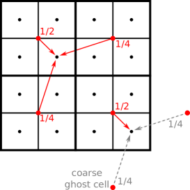
Figure 1: Illustration of the prolongation procedure in 2D. Cell-centered values on the coarse and fine grids are indicated by red and black circles, respectively. Arrows and weights indicate which coarse grid values are used for the interpolation. Near block boundaries, the interpolation makes use of coarse grid ghost cells, but note that no diagonal ghost cells are used. Formulas for the interpolation scheme are given in equations (6) and (7).

Besides a smoother, multigrid also requires prolongation and restriction methods, which transfer data from coarse to fine grids and vice versa. For prolongation we use linear interpolation based on the nearest neighbors, as is also included in e.g. the Boxlib [4] and Afivo [22] frameworks. The procedure is illustrated in figure 1 for a 2D case, and can be described by the following equations:

$$f_{x+h/4,y+h/4} =\frac{1}{4}\left(2f_{x,y}+f_{x+h,y}+f_{x,y+h}\right)+O(h^{2}),$$ (6)

$$f_{x-h/4,y+h/4} =\frac{1}{4}\left(2f_{x,y}+f_{x-h,y}+f_{x,y+h}\right)+O(h^{2}),$$

with the schemes for other points following from symmetry. In 3D, the interpolation stencil becomes

$$f_{x+h/4,y+h/4,z+h/4} =\frac{1}{4}\left(f_{x,y,z}+f_{x+h,y,z}+f_{x,y+h,z}+f_{x,y,z+h}\right)+O(h^{2}),$$ (7)

$$f_{x-h/4,y+h/4,z+h/4} =\frac{1}{4}\left(f_{x,y,z}+f_{x-h,y,z}+f_{x,y+h,z}+f_{x,y,z+h}\right)+O(h^{2}).$$

An advantage of these schemes is that they do not require diagonal ghost cells, which saves significant communication costs. A drawback is that interpolation errors can be larger than with standard bilinear or trilinear interpolation, somewhat reducing the multigrid convergence rate.

For restriction, the value of four (2D) or eight (3D) fine grid values is averaged to obtain a coarse grid value. Besides these built-in methods, users can also define custom prolongation and restriction operators.

2.4 Multigrid cycles

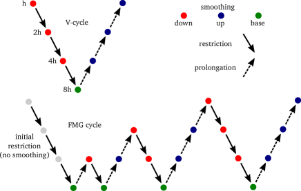
Figure 2: Schematic illustration of the V-cycle and FMG cycle for a grid with four levels. The FMG cycle contains several V-cycles at increasingly finer grids. At the start of an FMG cycle, the solution and the right-hand side are restricted to the coarsest grid.

Two standard multigrid cycles are included in the library [19, 18, 17]: the V-cycle and the full multigrid (FMG) cycle, which are illustrated in figure 2. As the name suggests, a V-cycle goes from the finest grid to the coarsest grid and then back to the finest grid. To explain the procedure, we introduce some terminology: let $v$ denote the approximate solution, $f$ the right-hand side, $L$ the elliptic operator, $r=f-Lv$ the residual, $P$ a prolongation operator, and $R$ a restriction operator. Furthermore, superscripts $h$ and $H$ refer to the current and the underlying coarse grid level.

During the downward part of the V-cycle, $N_{\mathrm{down}}$ (default: two) smoothing steps are performed at a grid level. Afterwards, the residual is computed as

$$r^{h}=f^{h}-L^{h}(v^{h}).$$

The current approximation $v^{h}$ is then restricted to the coarse grid as $v^{H}=R(v^{h})$, after which a copy $v^{H}_{\mathrm{old}}=v^{H}$ is stored. This copy is later used to update the fine-grid solution. The coarse-grid right-hand side is then updated as

$$f^{H}=R(r^{h})+L^{H}(v^{H}),$$ (8)

after which the procedure repeats itself, but now starting from the underlying coarse grid.

On the coarsest grid, up to $N_{\mathrm{max}}$ (default: 1000) smoothing steps are performed until the residual is either below a user-defined absolute threshold (default: $10^{-8}$), or until it is reduced by a user-defined factor (default: $10^{-8}$). When the coarsest grid contains a large number of unknowns, it can be beneficial to use a direct solver to solve the coarse grid equations, but we have not yet implemented this.

In the prolongation steps, the solution is updated with a correction from the coarse grid as

$$v^{h}=v^{h}+P(v^{H}-v^{H}_{\mathrm{old}}),$$ (9)

and afterwards $N_{\mathrm{up}}$ (default: two) smoothing steps are performed.

The FMG cycle consists of a number of V-cycles, as illustrated in figure 2. Compared to V-cycles, FMG cycles perform additional smoothing at coarse grid levels. This makes them a bit more expensive, but the advantage of FMG cycles is that they can achieve convergence up to the discretization error in one or two iterations.

If no initial guess for the solution is given, an initial guess of zero is used. We use the restriction and prolongation operators described in section 2.3 for both V-cycles and FMG cycles. Whenever necessary, for example after restriction/prolongation or after a smoothing step, ghost cells are updated, see section 2.6.

2.5 Grid structure

The library supports quadtree/octree grids with Cartesian 2D/3D or cylindrical 2D $(r,z)$ geometries, see e.g. [23]. Quadtree grids consist of blocks of $N_{x}\times N_{y}$ cells, which can be refined by covering them with four refined blocks (their ‘children’), which each also contain $N_{x}\times N_{y}$ cells but have half the grid spacing. An example of a quadtree grid is shown in figure 3. Octrees are the 3D equivalent of quadtrees, so that the refinement of a block creates eight ‘children’. The multigrid library requires that the difference in refinement between adjacent blocks is at most one level; such quadtree/octree grids are called 2:1 balanced.

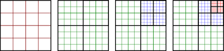
Figure 3: Example of a quadtree grid. Each black square represents a grid block containing $4\times 4$ cells. From left to right, the grid is refined in the upper right corner.

When the multigrid library is coupled to an application code, it constructs a copy of the full AMR hierarchy of the application code together with additional coarse grid levels. Applications codes therefore only need to contain fine grid data, and not the underlying coarse grid data. The library also contains its own routines for parallel communication and the filling of ghost cells, as described in sections 2.6 and 2.7.

The grid construction is performed in several steps. First, a user indicates the quadtree/octree block size and the size of the unrefined computational domain in the application code (in number of cells). The library will then internally construct additional coarse grid levels, as illustrated below. Afterwards, the refinement levels present in the application code are copied to the multigrid library.

2.5.1 Construction of additional coarse grids

Suppose that a 2D application uses blocks of $8^{2}$ cells and that its level one grid contains $192\times 96$ cells, see figure 4. The library will then first construct the additional coarse grids given in table 1. The block size is kept at $8\times 8$ down to level $-1$. For levels $-2$ to $-4$, the block size is reduced all the way down to $1\times 1$ blocks. These extra grids are constructed to obtain a coarsest grid with a small number of unknowns. On such a grid, a solution can directly be obtained with a modest number of iterations of the smoother. A coarsest grid with few unknowns can be obtained when the level one grid size is a small number (e.g., 1, 3 or 5) times a power of two.

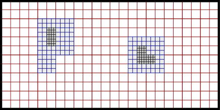
Figure 4: Example of a 2D grid with two levels of refinement, to help explain the construction of grids in the multigrid library. The base grid contains $192\times 96$ cells, which corresponds to $24\times 12$ blocks (shown in red) of $8\times 8$ cells. Table 1 lists the additional coarse grids that the multigrid library would construct.

grid level	mg	application	grid size	block size	$N_{\mathrm{blocks}}$
3	✓	✓	irregular	$8\times 8$	80
2	✓	✓	irregular	$8\times 8$	144
1	✓	✓	$192\times 96$	$8\times 8$	$24\times 12$
0	✓		$96\times 48$	$8\times 8$	$12\times 6$
-1	✓		$48\times 24$	$8\times 8$	$6\times 3$
-2	✓		$24\times 12$	$4\times 4$	$6\times 3$
-3	✓		$12\times 6$	$2\times 2$	$6\times 3$
-4	✓		$6\times 3$	$1\times 1$	$6\times 3$

Table 1: Example of the additional coarse grids that would be constructed for an unrefined domain of $192\times 96$ cells with blocks of size $8^{2}$, see figure 4. The check marks indicate whether the grid level is present in the multigrid library and in the calling application. $N_{\mathrm{blocks}}$ denotes the number of blocks per level in the multigrid hierarchy, so including blocks covered by refinement.

2.5.2 Copying the application’s grid refinement

After the unrefined (level one) grid has been constructed in the multigrid library, it can be linked to the application’s unrefined grid. In the application code, each grid block has to store an integer indicating the index of that grid block in the multigrid library. Similarly, grid blocks in the multigrid library store pointers to the application’s code grid blocks.

After the unrefined grids have been linked, the AMR structure can be copied from the application code by looping over its grid blocks, starting at level one. Refined blocks can be added to the multigrid library by calling built-in refinement procedures, after which these refined blocks again have to be linked between the two codes. An example of the coupling procedure can be found in the coupling module provided for MPI-AMRVAC.

2.5.3 Adapting the grid structure

When the mesh in the calling application changes, the mesh in the multigrid library can be adapted in the same way, or it can be constructed again from scratch. To adapt an existing mesh the calling application should inform the library about all blocks that were added, removed or transferred between processors (for load balancing, see section 2.7). The computational cost of constructing a new mesh is relatively modest: for the uniform-grid scaling tests in section 3.3, it took about $0.3\,\textrm{s}$ to construct a $1024^{3}$ grid consisting of octree blocks with $16^{3}$ cells.

2.6 Ghost cells and boundary conditions

In the multigrid library all grid blocks have a layer of ghost cells around them, which can contain data from neighboring blocks (potentially at a different refinement level) or special values for boundary conditions. The usage of ghost cells simplifies the implementation of numerical methods, since they do not need to take block boundaries into account. For simplicity and efficiency, the library currently uses only a single layer of ghost cells, without diagonal and/or edge (in 3D) cells. Since the multigrid library uses its own ghost cell routines, these restrictions do not apply to application codes, which can use any number of ghost cells.

The downside of ghost cells is that additional memory is required, as illustrated in table 2. Some AMR codes, such as Paramesh [24], therefore provide the possibility to compute ghost values when they are required instead of permanently storing them. However, this adds some complexity in the implementation of algorithms, for example because ghost cells cannot be reused in two separate steps.

block size	1 ghost cell	2 ghost cells	3 ghost cells
$8^{2}$	1.56	2.25	3.06
$16^{2}$	1.27	1.56	1.89
$32^{2}$	1.13	1.27	1.41
$8^{3}$	1.95	3.38	5.36
$16^{3}$	1.42	1.95	2.60
$32^{3}$	1.20	1.42	1.67

Table 2: Memory cost of using grid blocks of given size with ghost cells, relative to the cost without ghost cells. The values are computed as $(N+2N_{\mathrm{gc}})^{D}/N^{D}$, where $N$ is the block size, $N_{\mathrm{gc}}$ the number of ghost cells, and $D$ the problem dimension.

Ghost cells can be filled in three different ways. If there is a neighboring block (at the same refinement level), ghost cells are simply copied from the corresponding region. This is also performed at periodic boundaries.

Ghost cells near physical boundaries

If there is a physical boundary, ghost cells are set so that the boundary condition is satisfied at boundary cell faces. If the interior cell-centered value is $\phi_{i}$ and the ghost value is $\phi_{g}$, then a Dirichlet boundary condition $\phi=a$ at the cell face is set as $\phi_{g}=2a-\phi_{i}$. A Neumann boundary condition $\partial_{x}\phi=b$ is set as $\phi_{g}=\phi_{i}\pm h_{x}\,b$, where $h_{x}$ is the grid spacing and the sign depends on the direction the boundary is facing. For free space boundary conditions ($\phi\to 0$ for $r\to\infty$), we make use of a FFT-based solver to set boundary conditions, see section 2.8.

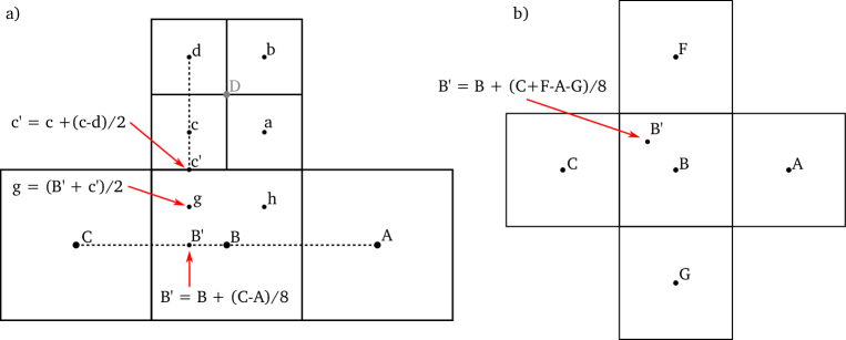
Figure 5: a) Illustration of the ghost cell scheme near a refinement boundary in 2D. Fine-grid values are indicated by a to d. The ghost cell next to c is located at g, and the nearest coarse-grid value is indicated by B. The quantities at B’ and c’ are shown to help explain how a value for g is obtained. Note that the coarse values A or C can be inside ghost cells of the block containing B; values at such ghost cells are always available in our implementation. b) In 3D, the procedure is almost identical. The only difference is how the equivalent of B’ is determined, which is illustrated here.

Ghost cells near refinement boundaries

Near refinement boundaries, we employ the scheme illustrated in figure 5a to fill ghost cells. The value B’ is obtained by using the central-difference slope in the coarse grid cell. The value at the cell face c’ is obtained by local extrapolation using two points, and finally the ghost cell value g is the average of B’ and c’. For the other ghost value h the procedure is geometrically identical. The approach extends naturally to 3D, in which two central-difference slopes are used in the coarse cells to obtain the equivalent of B’, as illustrated in figure 5b. An important property of this ghost cell scheme, which is similar to the scheme presented in [22], is that it gives the same coarse and (average) fine gradient across the refinement boundary. In other words, we have that

$$D-B=(c-g)/2+(a-h)/2,$$ (10)

where $D=(a+b+c+d)/4$ is the restriction of the fine cells. For a constant-coefficient Poisson equation such as (1), the divergence theorem

$$\int f\,dV=\oiint\varepsilon\nabla\phi\cdot\vec{dS}.$$ (11)

then shows that the integrated right-hand side is equal on the refined patch and on the underlying coarse grid approximation.

Near refinement boundaries, ghost cell values depend on the interior values of the refined block, as illustrated in figure 5. Since ghost cells are updated after (and not during) a smoothing step, a somewhat slower damping of errors is to be expected near refinement boundaries.

2.7 Parallelization

We have made a number of choices to keep the parallel implementation of the multigrid library relatively simple.

First, the full mesh geometry is stored on every processor. Of course, each processor only allocates storage for the mesh data that it ‘owns’. A more sophisticated approach would be to only store information about the local mesh neighborhood for each processor. That would save memory, but also significantly complicate e.g. mesh construction, mesh adaptation and load balancing.

Second, the multigrid library copies the mesh structure from the calling AMR application, and it is assumed that 2:1 balance is already satisfied.

Third, the load balancing is also copied from the calling AMR application, which means that all leaves (i.e., blocks with no further refinement) are on the same processors in the library as in the calling application. Copying data between the calling application and the library on the leaf blocks therefore involves no communication. This also means that the library only needs to perform load balancing for parent blocks. Our implementation assigns each parent block to the processor that contains most of its children, which is applied recursively by going from finer to coarser grids. In case of ties, the processor which has the fewest blocks at a refinement level is selected. This type of load balancing minimizes the communication between children and parent blocks.

On the coarsest grids in a multigrid hierarchy, there are too few unknowns to keep all processors busy. Furthermore, the cost of communication on such grids is often higher than computational costs. We therefore store the coarsest grids on a single processor, more precisely those for which the number of cells is not divisible by the block size. For the example of table 1, these are the grids with block size $4\times 4$ and smaller.

Parallel communication

As illustrated in figure 2, performing a multigrid cycle involves quite a lot of communication between processors. After performing a smoothing step, ghost cells have to be updated. Prolongation and restriction also require data to be transferred between grid levels, as well as an update of the ghost cells. For this reason, the multigrid library comes with efficient routines for filling ghost cells and communicating data.

The following data is communicated for the ghost cell, prolongation and restriction routines:

• For ghost cell exchanges at the same refinement level, the corresponding interior cell region is sent from both sides.

• For ghost cells near a refinement boundary, the coarse-side processor interpolates values ‘in front of’ the cells of its fine grid neighbor, see figure 5. These values are then sent from coarse to fine; there is no communication from fine to coarse.

• For prolongation, the coarse grid data is first interpolated and then sent to its children.

• For restriction, the fine grid data is first restricted and then sent to the underlying coarse grid.

For each of the above cases, the size of the data transferred depends only on the block size and the problem dimension. We avoid communication on the coarsest grids, for which the block size is reduced, since these grids are stored on a single processor.

The actual data transfer is performed using buffers, so that only a single send and/or receive is performed between communicating processors. The size of these buffers is computed after constructing the AMR grid; then it is known how much data is sent and received between processors in the various operations. Furthermore, the data in the send buffers is sorted so that it is in ‘natural’ order for the receiving processor. This sorting is possible because each grid block is identified by a global index, which determines the order in which processors loop over the blocks.

After the sorted data has been received, operations such as the filling of ghost cells, prolongation or restriction can be performed. Whenever data from another processor is required, it is unpacked from the buffer corresponding to that processor. If data from the same processor is required, it is locally prepared as described above. The advantage of this buffered approach for exchanging data is that it limits the number of MPI calls, which could otherwise lead to significant overhead. In section 3.3, we demonstrate the parallel scaling of our approach.

2.8 Free space boundary conditions in 3D

Poisson’s equation sometimes has to be solved with free space boundary conditions, i.e., $\phi\to 0$ at infinity, for example when computing the gravitational potential of an isolated system. Because of the $1/r$ decay of the free-space Green’s function, enlarging the computational domain (and applying a Dirichlet zero boundary condition) gives a poor approximation of the free-space solution.

A number of techniques exist to directly compute free-space solutions, see e.g. [25, 26]. The most efficient techniques rely on the fast Fourier transform (FFT), so they can only be applied to uniform grids. To incorporate free boundary conditions into our AMR-capable multigrid solver, we therefore employ the following strategy. First, a free-space solution is computed on a uniform grid, which can have a significantly lower resolution than the full AMR grid. Then standard multigrid is performed, using Dirichlet boundary conditions interpolated from the uniform grid solution.

We use the 3D uniform-grid solver described in [25, 27], which employs interpolating scaling functions and FFTs to obtain high-order solutions of free-space problems. The solver is written in Fortran, licensed under a GPL license, and it uses MPI-parallelism, which simplified its integration with our multigrid library.

In our implementation the uniform grid always corresponds to one of the fully refined grid levels (so excluding partially refined levels). Users can control the cost of the uniform grid solver with a parameter $c$, which should lie between zero and one. The uniform grid then corresponds to AMR level $l$ for which $N(l)\leq c\,N_{\mathrm{total}}$, where $N(l)$ denotes the number of unknowns at AMR level $l$, and $N_{\mathrm{total}}$ denotes the total number of unknowns.

After constructing the uniform grid, including a layer of ghost cells, the right-hand side of the problem is restricted to it. The direct solver then computes the free-space solution in parallel, using eight-order accurate interpolating scaling functions. We extract the boundary planes, and linearly interpolate them to obtain Dirichlet boundary conditions for the multigrid solver at all grid levels. Afterwards, one or more FMG or V-cycles can be performed to obtain a solution on the full AMR grid, using the uniform grid solution as an initial guess.

The coupled approach described above has two advantages: it can handle AMR grids, it can be more efficient and scale better than a direct solver, and it requires no modification of the multigrid routines. Potential drawbacks are that the multigrid solution is only second order accurate, and that the accuracy near boundaries is reduced when a too coarse grid is used for the direct solver. How fine the uniform grid needs to be compared to the full AMR grid depends on the application, e.g., on the distance between sources and the domain boundary, and on the required accuracy near the boundary.

3 Testing the library

3.1 Convergence test

To study the convergence behavior of the multigrid solver, we solve the following 3D test problem on a unit cube centered at the origin:

$$\nabla^{2}\phi =f,$$

$$f =\nabla^{2}\phi_{\mathrm{sol}},$$ (12)

$$\phi_{\mathrm{sol}} =\cos(\pi\vec{n}\cdot\vec{x})+10\exp(-100|\vec{x}|^{2}),$$

with $\vec{n}=(1,2,3)$. The right-hand side $f$ is computed analytically, and Dirichlet boundary conditions are imposed using the solution values at the boundary. We consider three types of numerical grid. The base case has uniform refinement using $64^{3}$ cells. To test the effect of refinement boundaries on the convergence behavior, we add two extra levels of refinement covering a volume of $0.5^{3}$ and $0.25^{3}$, respectively (so that each level again contains $64^{3}$ cells). These refinements are either placed at the center of the domain, or around $(-0.25,-0.25,-0.25)$. In the latter case, the refinement is in the ‘wrong’ place, as it leads to a refinement corner at the center of the domain, where the solution has a sharp peak.

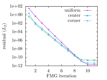
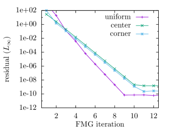
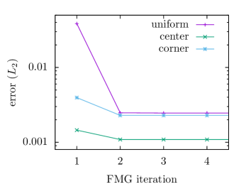
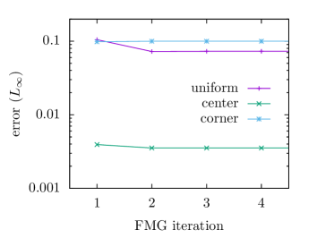
Figure 6: Convergence test results for the test problem of equation (3.1) with a sharp Gaussian peak. Top row: the residual in $L_{2}$ norm (left) and $L_{\infty}$ norm (right) versus FMG iteration. After about 10 iterations the residual is reduced up to machine precision, see the text for details. Bottom row: the $L_{2}$ norm and $L_{\infty}$ norm of the solution error. After two FMG iterations, the error has converged to the discretization error, which is why it is no longer decreasing. The uniform case contains $64^{3}$ cells, and the ‘center’ and ‘corner’ cases contain two additional levels of refinement, which if placed properly (the ‘center’ case) indeed decreases the error.

Figure 6 shows the residual $r=f-\nabla^{2}\phi$ versus FMG iteration. Two downward and two upward smoothing steps were taken per iteration. The residual reduction factor per iteration is reduced when refinement is present. This is a result of our ghost cell procedure near refinement boundaries, see section 2.6, which reduces the convergence rate. The residual is reduced up to machine precision after about 10 iterations. Due to the algorithmic steps involved, such as evaluating expressions like equation (3), the minimum residual that can be obtained is proportional to $\epsilon_{\mathrm{mach}}h^{-2}|\phi|$, where $\epsilon_{\mathrm{mach}}\approx 10^{-16}$ is the machine’s precision, $h$ is the mesh spacing and $|\phi|$ is the local amplitude of the computed solution.

Regardless of the lower reduction factor with refinement boundaries, figure 6 shows that the discretization error is reached in one or two FMG iterations. The test problem has a steep Gaussian at the center, which is where the largest discretization errors occur for the uniform grid case. With the centered refinement errors are indeed significantly reduced. In the $L_{\infty}$ norm, the error is reduced by a factor 20, slightly more than the factor 16 expected from a second-order discretization with two levels of refinement. With the corner refinement, the errors hardly change, showing that ‘wrongly’ placed refinements are handled well by our approach.

3.2 Free space solutions in 3D

To test our method with free space boundary conditions in 3D, see section 2.8, we solve a free space Poisson problem with a Gaussian right-hand side

$$\nabla^{2}\phi =f,$$ (13)

$$f(\vec{r}) =\frac{-1}{\sigma^{3}\pi^{3/2}}\exp(-|\vec{r}-\vec{r}_{0}|^{2}/\sigma^{2}),$$

where $\vec{r}_{0}$ is the center of the Gaussian and $\sigma$ controls its width. The solution is then given by

$$\phi(\vec{r})=\frac{1}{4\pi}\operatorname{erf}(|\vec{r}-\vec{r}_{0}|/\sigma)/|\vec{r}-\vec{r}_{0}|,$$ (14)

where $\operatorname{erf}$ denotes the error function. The computational domain is again a unit cube centered at the origin, and the Gaussian is located at the origin with $\sigma=0.1$. Figure 7 shows the $L_{2}$-norm of the error after two FMG cycles versus the grid resolution. Two curves are shown, for which the direct solver is called on levels $l_{\mathrm{max}}-1$ and $l_{\mathrm{max}}-2$ respectively, where $l_{\mathrm{max}}$ denotes the highest grid level. For grids larger than $64^{3}$, there is hardly any difference between the two curves, and they show second order convergence. For simplicity, uniformly refined grids are used, but the multigrid solver also works for AMR meshes.

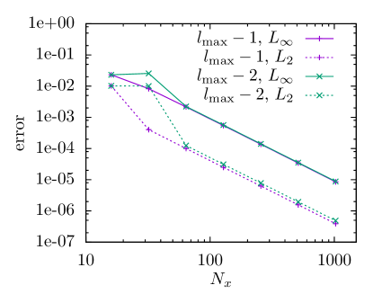
Figure 7: $L_{2}$ and $L_{\infty}$ norms of the error for the 3D free-space test problem given by equation (13). The error is shown versus the number of grid points per dimension. The labels $l_{\mathrm{max}}-1$ and $l_{\mathrm{max}}-2$ indicate at which grid level the direct free-space solver was called to obtain boundary conditions for the multigrid procedure, where $l_{\mathrm{max}}$ denotes the highest grid level.

The cost of the direct solver is relatively small, because it is only called once per right-hand side on a coarser grid, and because the direct solver itself is quite efficient [25].

3.3 Strong scaling tests

We now look at the performance and scaling of the geometric multigrid library, by solving Poisson’s equation with unit right-hand side

$$\nabla^{2}\phi=1,$$ (15)

on a unit cube, with $\phi$ set to zero at the boundaries. We measure the time per multigrid cycle for both FMG and V-cycles by averaging over 100 cycles. For both types of cycles two upward and two downward smoothing steps with a Jacobi smoother were performed, and octree blocks of size $16^{3}$ were used. The scaling results presented below were obtained on nodes with two 14-core Intel Xeon E5-2680v4 processors, for a total of 28 cores per node. In all tests, one MPI process per core was used. We present strong scaling results, which means that the problem size is kept fixed but the number of processors is increased.

Normally, the library copies its load balancing from another application, as discussed in section 2.7. For the tests presented below, the library was used by itself, in which case it performs a division of blocks over processors similar to a Morton order, which is also used in MPI-AMRVAC [28, 23].

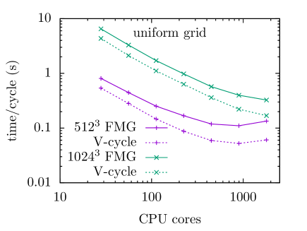
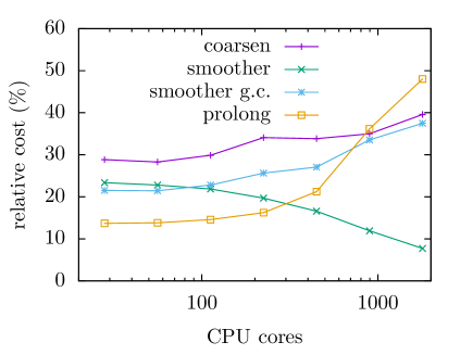
Figure 8: Left: strong scaling results for a problem size of $512^{3}$ and $1024^{3}$, showing the time per FMG cycle and per V-cycle. Right: breakdown of the computational cost of an FMG cycle for a $1024^{3}$ grid versus the number of CPU cores used.

Figure 8 shows strong scaling results for a uniform grid containing either $512^{3}$ or $1024^{3}$ cells. For the $512^{3}$ case, scaling results look good up to 448 cores, but with 1792 cores the performance is worse than with 896 cores. This makes sense: even on the finest grid, the number of unknowns is only about $42^{3}$ using 1792 cores. For the $1024^{3}$ test case, scaling is closer to ideal (i.e., closer to a straight line in the figure), even using 1792 cores. The figure also shows that the cost of a V-cycle is lower than that of an FMG cycle. The difference increases with the number of cores, due to the extra work on coarse grids with FMG cycles, see figure 2.

A breakdown of the relative cost of an FMG cycle for the $1024^{3}$ case is also shown in figure 8. Shown is the percentage of time spent on the transfer to coarse grids, the smoother (excluding communication), the ghost cell exchange during smoothing steps (labeled smoother g.c.), and the prolongation to finer grids. With an increasing number of cores, less time is spent on computation compared to communication.

Figure 9 shows strong scaling results on a refined grid with a total of five levels. Each grid level contains either $512^{3}$ or $1024^{3}$ cells, and the refinements are placed at the center of the domain, as illustrated in the figure. Compared to the uniform grid cases, there are about five times as many unknowns. The duration of V-cycles is indeed about five times longer, although the parallel scaling is improved due to the larger total number of unknowns. The difference in cost between V-cycles and FMG cycles is larger than for the uniform grid case, due to the extra work the FMG cycles perform on coarse grids, which now contain a significant number of unknowns.

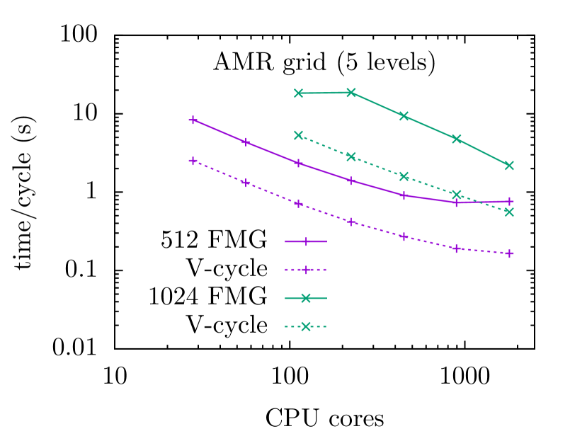
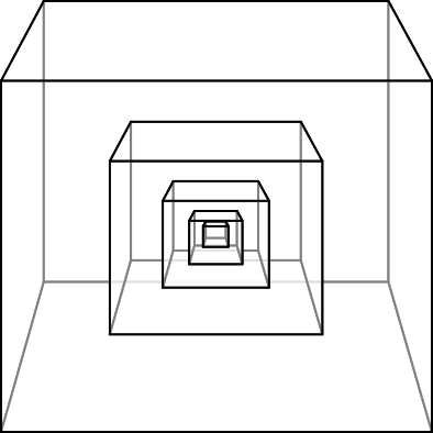
Figure 9: Strong scaling results on an AMR grid with 5 levels, with each level containing $512^{3}$ or $1024^{3}$ cells. The grid structure is illustrated on the right.

4 Divergence cleaning

This section is specifically about divergence cleaning in magnetohydrodynamic (MHD) simulations. For readers not interested in this particular application, we provide a short summary of the main results below:

• We compare elliptic, hyperbolic, and parabolic divergence cleaning for several test cases in 2D/3D Cartesian and $2.5$D cylindrical geometries, with AMR.

• With the multigrid library, divergence cleaning up to machine precision requires the magnetic field to be defined at cell faces. However, in MPI-AMRVAC the field is defined at cell centers, and we show that elliptic divergence cleaning can then still be applied successfully.

• We show that a fourth-order discretization of the right-hand side ($\nabla\cdot\vec{B}$) can be beneficial for elliptic divergence cleaning.

• The tests demonstrate the coupling of the multigrid solver to MPI-AMRVAC. The cost of runs was not significantly increased (by less than 10%) when elliptic divergence cleaning was performed once per time step.

• The tests show that for typical problems, divergence cleaning methods play a similar role as the slope limiters: different methods give slightly different results and there is no single best method.

Maxwell’s equations state that $\nabla\cdot\vec{B}=0$, but this constraint does not automatically hold in numerical MHD computations [29]. If no special care is taken, $\nabla\cdot\vec{B}$ can grow at each step through discretization errors, leading to unphysical results. Therefore, a number of methods has been developed to ensure $\nabla\cdot\vec{B}$ remains small compared to discretization and truncation errors.

With the Hodge–Helmholtz projection method [29, 30], the divergence is cleaned by solving Poisson’s equation:

$$\nabla\cdot\nabla\phi=\nabla\cdot\vec{B}_{\mathrm{old}},$$ (16)

$$\vec{B}_{\mathrm{new}}=\vec{B}_{\mathrm{old}}-\nabla\phi.$$ (17)

Below, we call this approach elliptic divergence cleaning, and we will use multigrid to solve Poisson’s equation. Another approach is to add source terms to the MHD equations to control $\nabla\cdot\vec{B}$ errors, as is done in the eight-wave formulation of Powell [31], or its variants which only affect the induction equation [32, 33]. The MHD equations can also be modified to ensure transport and/or damping of $\nabla\cdot\vec{B}$ errors. The extra terms can have a parabolic (diffusive) character, as in the ‘diffusive’ method described in [34] which only adds a diffusion term to the induction equation. When using an extended version of the MHD equations with a variable that links to $\nabla\cdot\vec{B}$ error damping and transport, the method can also have a hyperbolic character, as in the Generalized Lagrange multiplier (GLM) method described in [35] and the recently derived ideal GLM-MHD scheme presented in [36].

Constrained transport (CT) methods [37, 38, 39] were designed to preserve $\nabla\cdot\vec{B}=0$ up to machine precision, typically by defining the magnetic field at cell faces and the electric field at cell corners. Variants that do not rely on a staggered representation of the magnetic field have been discussed in [40] . CT methods have been made compatible with adaptive mesh refinement [41, 42, 43, 44, 45], but their implementation is non-trivial. Moreover, while CT methods ensure one particular discretization of the monopole constraint in machine precision, any other discretization will show truncation errors in places of large gradients, and especially at discontinuities. For mesh-free computations, [46] recently advocated the use of a constrained-gradient method, which in essence uses an iterative least-square minimization involving the magnetic field gradient tensor. Mesh-free smoothed-particle MHD implementations have also successfully devised constrained hyperbolic/parabolic divergence cleaning methods, where the wave cleaning speeds become space and time dependent [47].

An extensive comparison of $\nabla\cdot\vec{B}$ cleaning techniques was performed in [40], where a suite of rigorous test problems on uniform Cartesian grids showed that a projection scheme could rival central difference and constrained transport schemes in accuracy and reliability. Further comparisons have been performed in e.g. [48, 4], where especially [48] demonstrates some deficiencies in using divergence cleaning steps versus CT, when applied to supernova-induced MHD turbulence.

In the tests below, we compare elliptic, parabolic and hyperbolic divergence cleaning. ‘Elliptic’ refers to the multigrid-based projection method described in the next section, ‘parabolic’ to the diffusive approach of [34], and ‘hyperbolic’ to the EGLM-MHD method described in [35]. For the EGLM-MHD approach, we set the parameter $c_{h}$ to the globally fastest wave speed, and we use $c_{p}^{2}/c_{h}=2h$ to balance decay and transport of the $\psi$ variable, where $h$ is the finest grid spacing.

Below, a suffix 4^th indicates that $\nabla\cdot\vec{B}$ terms have been computed with a fourth-order accurate scheme, which is relevant for the elliptic and parabolic methods.

4.1 Elliptic divergence cleaning

In MPI-AMRVAC, the magnetic field is defined at cell centers. To compute its divergence in a Cartesian geometry, we consider two discretizations for $\nabla\cdot\vec{B}=\partial_{x}B_{x}+\partial_{y}B_{y}+\partial_{z}B_{z}$. Each derivative can either be approximated with second order central differences

$$\partial_{x}B_{x}\approx\frac{B_{x,i+1}-B_{x,i-1}}{2\Delta x},$$ (18)

or with a fourth-order differencing scheme

$$\partial_{x}B_{x}\approx\frac{-B_{x,i+2}+8B_{x,i+1}-8B_{x,i-1}+B_{x,i-2}}{12\Delta x}.$$ (19)

Afterwards, we update the magnetic field according to equation (17), and update the energy density as

$$e_{\mathrm{new}}=e_{\mathrm{old}}+\frac{1}{2}\left(B^{2}_{\mathrm{new}}-B^{2}_{\mathrm{old}}\right),$$ (20)

which keeps the thermal pressure constant [40], which can be important to avoid negative pressures. A downside is that equation (20) does not conserve total energy. For the correction step, we evaluate $\nabla\phi$ with second-order central differences.

The multigrid solver described in this paper is cell-centered, and with its standard 5/7-point stencil the divergence $\nabla\cdot\nabla\phi$ is computed from a face-centered quantity ($\nabla\phi$). Since in MPI-AMRVAC $\nabla\cdot\vec{B}$ is the divergence of a cell-centered quantity, the two divergences do not exactly match. This means that after the projection step, $\nabla\cdot\vec{B}$ will be non-zero in both the second and fourth order schemes, although differences will be small for smooth profiles. Based on the results presented here and those of [40], we think this is not necessarily a problem.

With a staggered discretization, in which the magnetic field is defined at cell faces, the two divergences in equation (16) exactly match. Divergence cleaning can then be performed up to machine precision. The multigrid library is currently used in the BHAC code [45], which employs such a staggered discretization, to ensure that initial magnetic fields are divergence-free up to machine precision.

4.2 Field loop advection

We first consider the 2D field loop advection test described in [49], which was also used more recently in e.g. [46]. A weak magnetic field loop is advected through a periodic domain given by $x\in[-1,1]$ and $y\in[-1/2,1/2]$. The initial conditions are $\rho=1$, $p=1$, $(v_{x},v_{y})=(2,1)$, and the magnetic field is computed from a vector potential whose only non-zero component is

$$A_{z}=\begin{cases}A_{0}(R_{0}-\sqrt{x^{2}+y^{2}})&\text{for }x^{2}+y^{2}\leq R_{0}^{2}\\ 0&\text{for }x^{2}+y^{2}>R_{0}^{2}\end{cases},$$

where $A_{0}=10^{-3}$ and $R_{0}=0.3$. We numerically evaluate $B_{x}=\partial_{y}A_{z}$ and $B_{y}=-\partial_{x}A_{z}$ using second-order central differencing. Inside the magnetized field loop the plasma beta is $\beta=2p/B^{2}=2\cdot 10^{6}$, so that this is effectively a hydrodynamics problem in which the magnetic field is a passive scalar. Nevertheless, its solution can be sensitive to the divergence cleaning method used [49, 46].

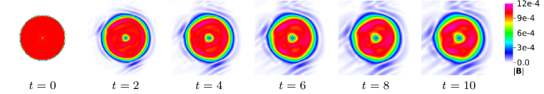
Figure 10: Example of the evolution of the magnetic field strength for the advected field loop test with parabolic divergence cleaning and the Čada slope limiter. At $t=10$, the loop has translated 10 times (horizontally and vertically). The figures show half of the computational domain, namely $x\in[-1/2,1/2]$ and $y\in[-1/2,1/2]$.

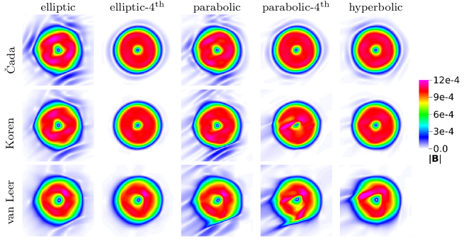
Figure 11: Magnetic field strength at $t=10$ for the advected field loop test. The columns correspond to different divergence-cleaning methods, and a suffix 4^th indicates a fourth-order scheme is used to evaluate $\nabla\cdot\vec{B}$ terms. The rows correspond to different slope limiters. The figures show half of the computational domain, namely $x\in[-1/2,1/2]$ and $y\in[-1/2,1/2]$.

We simulate this system up to $t=10$ on a uniform $256\times 128$ grid (AMR tests follow in the next subsection), with a grid spacing $h=1/128$. An example of the evolution is shown in figure 10, which was obtained using the parabolic approach. Fluxes were computed with the HLL scheme, using a CFL number of $0.5$. For figure 10, a Čada limiter [50] was used to reconstruct cell face values for flux computations. At $t=10$, the field loop has moved through the system 10 times. We run simulations with several combinations of slope limiters and $\nabla\cdot\vec{B}$ methods, always employing the same HLL scheme. These slope limiters are used in MPI-AMRVAC to reconstruct cell-face values from cell-centered ones for the flux computation [23]. Figure 11 shows the magnetic field strength $|\vec{B}|$ at $t=10$ for three types of limiters, described in [50] (‘Čada’), [51] (‘Koren’), and [52] (‘van Leer’), for five different cleaning approaches.

The computational cost of the MPI-AMRVAC runs hardly depended on the divergence cleaning method that was used, with run times differing by less than 10%. The choice of limiter had a greater impact. Runs with the more complex ‘Čada’ limiter took up to 40% longer than those with the simple van Leer limiter (which is symmetric), and runs with the Koren limiter were in between.

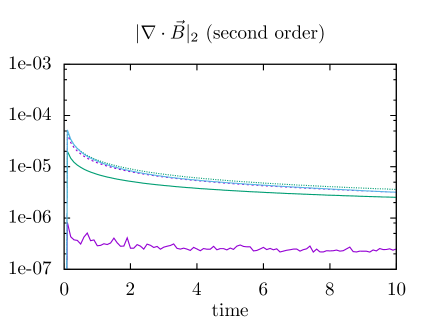
Figure 12: The $L_{2}$-norm of $\nabla\cdot\vec{B}$ versus time for the advected field loop test on a uniform $256\times 128$ grid. We only show the results for the Čada limiter. On the left, the $L_{2}$-norm is computed using a second order scheme for $\nabla\cdot\vec{B}$, on the right using a fourth order scheme.

With a second-order evaluation of $\nabla\cdot\vec{B}$, elliptic and hyperbolic divergence cleaning give similar results, somewhat worse than those obtained with hyperbolic cleaning. With a fourth-order evaluation of $\nabla\cdot\vec{B}$, elliptic cleaning gives the best results, which also appear to be less sensitive to the limiter used. It is to be noted that more structure is visible in Fig. 11 outside the loop than shown in e.g. [46], but this is due to the combination of using a different color scheme (our color legend is indicated in the figure), and because we show $|\vec{B}|$ instead of $B^{2}$.

Figure 12 shows the $L_{2}$-norm of $\nabla\cdot\vec{B}$, defined as

$$|\nabla\cdot\vec{B}|_{2}=\sqrt{\frac{1}{V}\int|\nabla\cdot\vec{B}|^{2}dV},$$ (21)

using a second-order and a fourth-order cell-centered evaluation. The elliptic schemes give the smallest $|\nabla\cdot\vec{B}|_{2}$ when the same second/fourth-order discretization is used to evaluate $|\nabla\cdot\vec{B}|_{2}$ and the right-hand side of Eq. (16). However, $\nabla\cdot\vec{B}$ being small in one discretization does not mean it is small in another one, as was as observed in [40].

The $L_{2}$-norm of $|\vec{B}-\vec{B}_{\mathrm{sol}}|$ is shown in figure 13, where $\vec{B}_{\mathrm{sol}}$ is the approximate solution to the problem, only taking into account advection of the initial condition. From this comparison, the elliptic-4^th and parabolic-4^th schemes give the best results, whereas the standard elliptic and parabolic schemes perform a bit worse than other methods. Since the cost of a fourth-order evaluation of $\nabla\cdot\vec{B}$ is negligible, the results suggest that such an evaluation can be recommended. In conclusion, we find that elliptic divergence cleaning works well to control monopole errors for this test case.

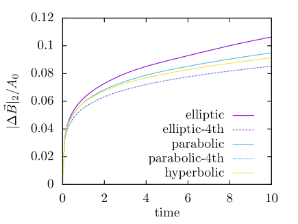
Figure 13: The $L_{2}$-norm of the error in the magnetic field $|\vec{B}-\vec{B}_{\mathrm{sol}}|$ divided by the initial amplitude $A_{0}=10^{-3}$, shown for the advected field loop test with the Čada limiter.

4.3 Advecting a current-carrying cylinder (mach 0.5)

Although the previous setup became a popular test for magnetic divergence control, it is not a realistic test case for MHD applications since it only probes the very high plasma beta (order one million to infinity) regime. Moreover, the initial condition is not a true MHD equilibrium, has an infinite current at $r=0$ together with a current sheet at its boundary $R_{0}$, and the radially inward Lorentz force must actually set up sausage type compressions of the loop, which could well be responsible for the fluctuations seen in the environment of the advected loop in Fig. 10.

Below, we introduce a more realistic advection test, which can be used to demonstrate a number of typical computational challenges in MHD applications: (1) combining high and low plasma beta regimes, (2) ensuring force balance, and (3) handling surface current contributions in AMR evolutions.

4.3.1 Description of the general test case

We set up a current-carrying magnetic flux tube embedded in a uniform, magnetized external medium, ensuring that a true MHD equilibrium is realized. This is then further combined with a uniform flow field, that addresses whether Galilean invariance is obtained.

Using the scale invariance of the MHD equations [53], we exploit units where the radius of the flux tube is equal to unity, where the density external to the loop is fixed at $\rho_{\mathrm{ext}}=1$, while the external plasma pressure is $p_{\mathrm{ext}}=1/\gamma$. This makes the external sound speed and its unit length crossing time the reference speed and time unit, respectively. The initial flow field is then controlled fully by its Mach number $M_{0}$ and orientation angles $\varphi_{0}$ and $\theta_{0}$, such that the constant speed components are found from

$$v_{x}(t=0) = M_{0}\sin\theta_{0}\cos\varphi_{0}\,,$$ (22)

$$v_{y}(t=0) = M_{0}\sin\theta_{0}\sin\varphi_{0}\,,$$ (23)

$$v_{z}(t=0) = M_{0}\cos\theta_{0}\,.$$ (24)

We align the flux tube with the $z$-direction, and use a $[-L,L]^{2}$ fully periodic domain, where we resort to a 2.5D (invariance in $z$) computation, although the problem can also be simulated in full 3D. The external medium has a uniform magnetization, which is determined by the corresponding inverse plasma beta parameter $\beta_{\mathrm{ext}}^{-1}$ as $B_{z,\mathrm{ext}}=\sqrt{2\beta_{\mathrm{ext}}^{-1}/\gamma}$.

The flux tube itself has internal variation, and is a force-free cylindrical equilibrium introduced in [54], where the physics of solar flares was discussed. For solar coronal applications, ensuring a force-free equilibrium, which guarantees $\vec{J}\times\vec{B}=\vec{0}$ without enforcing a vanishing current $\vec{J}=\nabla\times\vec{B}$, is a typical computational challenge. The internal variation for $r=\sqrt{x^{2}+y^{2}}\leq 1$ is given by

$$\rho_{\mathrm{int}}(r) = \rho_{0}(1-(1-d)r^{2})\,,$$ (25)

$$B_{z,{\mathrm{int}}}(r) = \frac{B_{0}}{1+c^{2}r^{2}}\,,$$ (26)

$$B_{\theta,{\mathrm{int}}}(r) = \frac{crB_{0}}{1+c^{2}r^{2}}\,.$$ (27)

The parameters $\rho_{0}$, $B_{0}$ and $c$ are best controlled by dimensionless numbers which quantify the pitch and strength of the magnetic field variation. The $d$ parameter quantifies the internal density contrast $d=\rho(1)/\rho(0)$. Introducing the $q$-factor at the tube radius

$$q(1)=\frac{\pi B_{z}(1)}{LB_{\theta}(1)},$$

along with the plasma beta at the flux tube radius $\beta(1)$, as well as the ratio $R$ of the Alfvén speed at $r=0$ to the external sound speed, we can deduce that

$$c = \frac{\pi}{Lq(1)}\,,$$ (28)

$$p_{\mathrm{int}} = \frac{\beta(1)(1+\beta_{\mathrm{ext}}^{-1})}{\gamma(\beta(1)+1)}\,,$$ (29)

$$B_{0} = \sqrt{\frac{2p_{\mathrm{int}}(1+c^{2})}{\beta(1)}}\,,$$ (30)

$$\rho_{0} = \frac{B_{0}^{2}}{R^{2}}\,.$$ (31)

The flux tube is internally force-free and represents a nonlinear force-free field configuration where $\vec{J}=[2c/(1+c^{2}r^{2})]\vec{B}$, while there is a constant pitch $q(r)=q(1)$. The embedded configuration is fully force-balanced since the above relations enforce the total pressure balance across the loop radius.

Any combination of input parameters $M_{0}$, $\theta_{0}$, $\varphi_{0}$, $\beta_{\mathrm{ext}}^{-1}$, $q(1)$, $\beta(1)$, $d$, and $R$ represents a meaningful test for which the exact solution is known: the flux tube will be advected at the prescribed constant speed. These parameters could explore regimes that are particularly challenging for numerical treatments, like taking the pitch such that the flux tube is liable to kink instability, or advecting at highly supersonic speeds, or verifying very low beta behavior, etc. The edge of the flux tube carries a surface current, where density, pressure and magnetic field components change discontinuously. This is typical for many solar, astrophysical or laboratory plasma configurations.

4.3.2 Results for a particular sets of parameters

We here focus on the particular case where $L=2$, $d=0.05$, $M_{0}=0.5$ (i.e. Mach 0.5 advection), $\phi_{0}=45^{\circ}$, $\theta_{0}=70^{\circ}$, $\beta(1)=0.05$ (i.e. a truly low beta flux tube), $q(1)=1.2$ (such that it is stable to external kink modes through the Kruskal–Shafranov limit), $R=1$, and taking $\beta_{\mathrm{ext}}^{-1}=0.05$ (i.e. a high beta surrounding medium). We perform 2.5D simulations using a three-step Runge-Kutta integrator with the HLL scheme combined with a Koren limiter, and a Courant parameter of $0.8$. Parabolic and elliptic divergence cleaning is applied, using a fourth order discretization of $\nabla\cdot\vec{B}$ terms. We use a base resolution per direction of 128 with four grid levels, which effectively gives a $1024^{2}$ resolution. We run until normalized time $t=10$, at which time the flux tube is almost advected back to its original position. Grid refinement is handled as follows: we enforce the maximal refinement level to resolve the region that is initially between $0.9<r<1.1$, to accurately treat the surface discontinuities during the entire evolution.

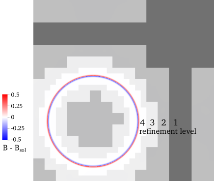
Figure 14: The error in the magnetic field magnitude at $t=10$ for the Gold–Hoyle force-free flux rope advection test, shown in the full $[-2,2]^{2}$ domain. The errors are localized at the surface of the flux rope, where there is a surface current and a jump in density. The figure shows results for the multigrid approach (elliptic-4th). The four refinement levels are indicated by gray-to-white colors, with the finest (white) grid having a spacing of about $4\times 10^{-3}$.

Figure 14 shows the error in the magnetic field strength at $t=10$ using elliptic divergence cleaning. The error is concentrated at the boundary of the flux rope, where there is a surface current and a jump in density. The grid structure at $t=10$ is also shown in figure. With the parabolic approach, the results are nearly identical.

Figure 15 shows the average magnitude of $\vec{J}\times\vec{B}$ in the region inside, outside and at the boundary of the flux rope. Results are shown for both the elliptic and parabolic approach, but only small differences between the two methods can be observed. Note that the simulation is nearly force-free inside and outside the flux rope. At the edge of the flux rope $\vec{J}\times\vec{B}$ is significantly larger, due to the numerical discretization errors at the flux rope boundary.

We remark that with hyperbolic divergence cleaning, we obtain nearly identical results. In conclusion, this test case shows that for a physically realistic test case, the type of divergence cleaning has less effect than for the test problem of section 4.2. It also demonstrates that our divergence cleaning methods, and more specifically the elliptic approach, can handle adaptive mesh refinement.

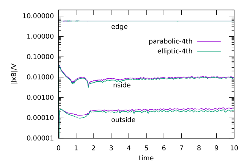
Figure 15: The average magnitude of $\vec{J}\times\vec{B}$ in three regions: the region outside the flux rope ($r>1.1$), the region inside the flux rope ($r<0.9$) and the region in between ($0.9<r<1.1$), where $r=0$ corresponds to the center of the flux rope.

4.4 Modeling magnetized jets (2.5D and 3D)

A final demonstration of the multigrid-based divergence cleaning methodology focuses on a typical astrophysical application: the propagation of a strongly magnetized, supersonic and super-Alfvénic jet. We perform both 2.5D axisymmetric and 3D Cartesian simulations. The configuration is borrowed from [55], where relativistic jets with helical field topologies were studied in axisymmetry. We here use the same magnetic field topology in the initial conditions, and evolve purely Newtonian cases, so we take parameters similar to the non-relativistic jet case from [55].

4.4.1 Description of the test case

At $t=0$, the jet occupies a finite region $R<R_{j}$ and $Z<Z_{j}$ where the (normalized) density is $\rho_{j}=1$, while the surrounding medium has a higher density $\rho_{c}=10$: the under-dense jet is entering a denser ‘cloud’ region. We take the domain size as follows: $R\in[0,30]$ and $Z\in[0,90]$, while $R_{j}=1.5$ and $Z_{j}=3.0$. The jet itself has a twisted field topology with an azimuthal field component in the jet region given by

$$B_{\varphi}=\tanh\frac{R}{5}\,,$$ (32)

while this azimuthal field vanishes in the surroundings. Note again how this setup thereby necessarily involves surface current distributions (located at the edge of the jet region). The other magnetic field components are

$$B_{R} = 2\frac{R_{j}}{Z_{j}}\frac{\left(\frac{Z}{Z_{j}}\right)^{3}\tanh\left(\frac{Z}{Z_{j}}\right)^{4}\tanh\left(\frac{R}{R_{j}}\right)^{2}}{\frac{R}{R_{j}}\cosh\left(\frac{Z}{Z_{j}}\right)^{4}}\,,$$ (33)

$$B_{Z} = B_{c}+\frac{1}{\left[\cosh\left(\frac{R}{R_{j}}\right)^{2}\right]^{2}\cosh\left(\frac{Z}{Z_{j}}\right)^{4}}\,.$$ (34)

This magnetic field setup is analytically divergence-free (as it should), and ensures that the jet is entering an almost uniformly magnetized cloud region where the initial field strength has the ‘cloud’ value $B_{c}=0.01$. The initial pressure distribution follows from

$$p=p_{j}+\frac{1}{2}-\frac{1}{2}\left(B_{\varphi}^{2}(R,Z)+B_{Z}^{2}(R,Z)\right)\,,$$ (35)

where we take the jet pressure parameter $p_{j}=2$: this makes the internal jet region slightly under-pressured with respect to the external medium, and an order of magnitude hotter than its surroundings. Finally, the flow field $\vec{v}$ vanishes at $t=0$ outside the jet region, but within the jet follows from

$$v_{R} = 0\,,$$ (36)

$$v_{Z} = \alpha\frac{B_{\varphi}}{(R/5)\sqrt{\rho_{j}}}\,,$$ (37)

$$v_{\varphi} = \frac{B_{\varphi}}{\sqrt{\rho_{j}}}\,.$$ (38)

The parameter $\alpha=6.0$. These choices turn the jet Mach number $v_{Z}/c_{s}\approx 3$ while its Alfvén Mach number $v_{Z}/v_{A}\approx 6$ (both of these quantities vary with radius and relate to the local sound speed $c_{s}=\sqrt{\gamma p/\rho}$ and Alfvén speed $v_{A}=B/\sqrt{\rho}$). The ratio of specific heats is fixed at $\gamma=5/3$. In accord with the frequently invoked equipartition argument for astrophysical jets, the plasma beta internal to the jet is of order $\beta=2p/B^{2}\approx 4$, while it is about 50000 in the cloud region.

4.4.2 Computational domain and refinement

In 2.5D, the resolution uses a coarse $32\times 64$ base grid, allowing a total of 6 AMR levels (i.e. an effective resolution of $1024\times 2048$). Refinement uses the Lohner estimator, this time taking in weighted information from $\rho$, $m_{R}=\rho v_{R}$ and $B_{\varphi}$ in a $0.5-0.25-0.25$ ratio. Maximal resolution is enforced within the region $R<3R_{j}$ and $Z<3Z_{j}$. Boundary conditions use the usual (a)symmetric combinations to handle the $R=0$ symmetry axis and extrapolate all variables at side and top in a zero-gradient fashion. The bottom boundary uses the analytic initial conditions within $R<R_{j}$, and adopts a reflective boundary beyond.

In 3D, our setup adopts the same physical parameters, but this time in a 3D Cartesian $(x,y,z)$ box of size $[-30,30]\times[-30,30]\times[0,90]$, where the $z$ axis coincides with the symmetry axis employed in the 2.5D runs (making $R=\sqrt{x^{2}+y^{2}}$). To avoid an artificial $m=2$ selection effect in the way non-axisymmetric modes with azimuthal mode number $m\neq 0$ develop from the noise (inherent to doing cylindrical problems on a Cartesian grid), we used a deterministic incompressible velocity perturbation consisting of 7 mode numbers $m=1,\ldots,7$ derived from $\psi=\sum_{m}A_{m}\cos(m\varphi+\phi_{m})\exp(-[(R-0.75R_{j})/R_{j}]^{2})$ such that $\delta\vec{v}=\nabla\times\psi(x,y)\hat{e}_{z}$. This is applied in the ghost cells at the bottom ($z=0$) boundary only, where we add it to the fixed velocity field providing the jet conditions. The 7 amplitudes are chosen such that a maximal amplitude for each mode is $A_{m}\leq 0.05$. In 3D, our base resolution is $64\times 64\times 96$, with 5 refinement levels to get to $1024\times 1024\times 1536$ effectively. Refinement in 3D is based on density only, augmented with user-enforced geometric criteria, where e.g. the maximal resolution is always attained within the region $R<3R_{j}$ and $Z<3Z_{j}$. Boundary conditions at all sides and top extrapolate primitive variables using Neumann zero-gradient prescriptions. The bottom boundary fixes the entire initial condition, augmented with the $\delta\vec{v}$ addition, within the jet zone, while reflective boundaries are used beyond $R>R_{j}$.

4.4.3 Results

We run till time $t=60$, such that the jet progressed up to about $z\approx 60$. We use a strong-stability preserving Runge-Kutta scheme (its implementation in MPI-AMRVAC is demonstrated in [3]), an HLLC discretization, and Piecewise Parabolic (PPM) reconstruction. Runs differ only in their divergence cleaning approach. We anticipate many turbulent features related to fluid instabilities, waves, rarefactions and shocks, as typical for under-dense supersonic jets, but all differences in the jet morphology here entirely relate to the error control on magnetic monopoles.

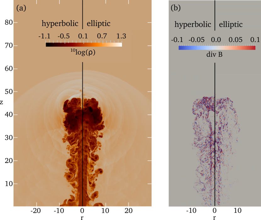
Figure 16: (a) The logarithm of the density at $t=60$ for the helically magnetized jet in axisymmetric conditions, using the hyperbolic (left) versus the multigrid-based elliptic (right) treatment for monopole control. (b) The numerical value of $\nabla\cdot\vec{B}$, evaluated with a second order central difference formula, at $t=60$ for the hyperbolic and elliptic approach.

In Fig. 16(a), we show the density distribution for the axisymmetric simulations at $t=60$, comparing the hyperbolic with the elliptic method for divergence control. Naturally, many details differ between the two cases, although both recover the richness in internal jet beam shocks, fluid instabilities developing at the leading contact interface between jet and surroundings, and the turbulent backflows where many vortical structures exist. The shocked cloud matter is riddled with shocks. Repeated deformations of the contact interface shed plasma into the backflow surrounding the jet spine.

A direct comparison of the monopole errors at $t=60$ is given in Fig. 16(b). We here show a second order central difference evaluation of $\nabla\cdot\vec{B}$ (we also used the second order evaluation of the source term in the cleaning methods). With the elliptic cleaning there are fewer cells with significant $\nabla\cdot\vec{B}$ values. All monopole errors concentrate near the many discontinuities, as expected. Overall, the jet progressed to about the same distance.

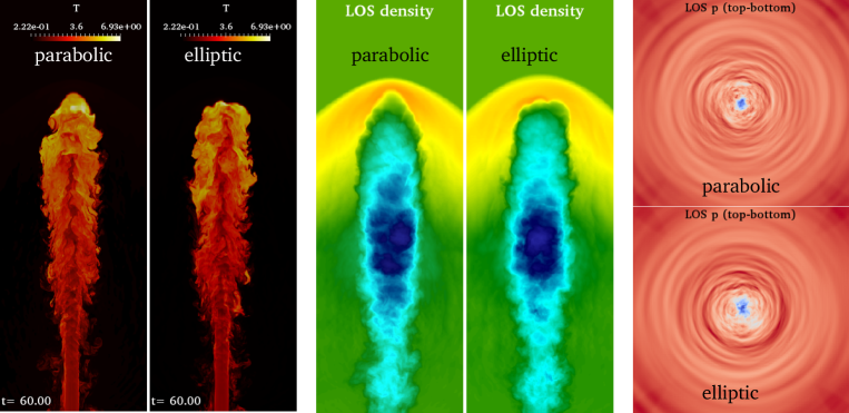
Figure 17: Several views on the 3D jet simulation at $t=60$, where we used the parabolic and elliptic approach for divergence control. We show a cross-section of the temperature (left), a line-integrated side view of the density (middle) and a line-integrated top view of the pressure (right).

The same simulation in full 3D allows for non-axisymmetric deformations, which can come about from current-driven kink instabilities mediated by the helical magnetic field of the jet, or by the many shear-flow driven events. The state at $t=60$ is shown in Fig. 17, where we now compare the elliptic approach to the parabolic one. The cross-sectional temperature view (left), and the line-of-sight integrated density views (middle) cover the full extent in $z\in[0,90]$, while the integrated pressure view shows the entire $x-y$ cross-section $[-30,30]^{2}$. The turbulent cocoon that develops around the jet spine aids in retaining a coherent jet over the distance simulated: the turbulence in the backflow region seems to prevent large deformations of the jet. The overall morphology of the 3D helical jet is very similar with both monopole corrections. A more in-depth discussion of the physics in the context of astrophysical jet propagation is deferred to future work. Fig. 17 shows that the temperature, density, and pressure variations are all very well recovered with either method for monopole control.

5 Conclusions

We have presented an MPI-parallel geometric multigrid library. The library can be used to extend octree-based adaptive mesh refinement frameworks with an elliptic solver. The library supports multigrid V-cycles and FMG cycles, and employs standard second-order discretizations. Cartesian 2D/3D and cylindrical 2D grid geometries can be used, with periodic, Dirichlet, or Neumann boundary conditions. For 3D Poisson problems free-space boundary conditions are also supported, by using an FFT-based solver on the coarse grid. The convergence and scaling of the library has been demonstrated with multiple test problems.

We have demonstrated the coupling of the library to MPI-AMRVAC, an existing AMR code, by using the multigrid routines for divergence cleaning in MHD simulations. We have compared three approaches: elliptic, hyperbolic and parabolic divergence cleaning. Several test cases were presented, in 2D and 3D Cartesian as well as axisymmetric geometries. Elliptic divergence cleaning (i.e., using a projection method) was found to work satisfactorily in all cases, although the other methods generally performed similarly well.

Acknowledgments

JT is supported by postdoctoral fellowship 12Q6117N from Research Foundation – Flanders (FWO). RK acknowledges support by FWO-NSFC grant G0E9619N.

The computational resources and services used in this work were provided by the VSC (Flemish Supercomputer Center), funded by the Research Foundation – Flanders (FWO) and the Flemish Government – department EWI.

References

-
[1]
A. Gholami, D. Malhotra, H. Sundar, G. Biros,
FFT, FMM, or multigrid? A
comparative study of state-of-the-art Poisson solvers for uniform and
nonuniform grids in the unit cube, SIAM Journal on Scientific Computing
38 (3) (2016) C280–C306.
doi:10.1137/15m1010798.
URL http://dx.doi.org/10.1137/15M1010798 -
[2]
C. Xia, J. Teunissen, I. E. Mellah, E. Chané, R. Keppens,
MPI-AMRVAC 2.0 for solar
and astrophysical applications, The Astrophysical Journal Supplement Series
234 (2) (2018) 30.
doi:10.3847/1538-4365/aaa6c8.
URL http://dx.doi.org/10.3847/1538-4365/aaa6c8 -
[3]
O. Porth, C. Xia, T. Hendrix, S. P. Moschou, R. Keppens,
MPI-AMRVAC for solar and
astrophysics, The Astrophysical Journal Supplement Series 214 (1) (2014) 4.
doi:10.1088/0067-0049/214/1/4.
URL http://dx.doi.org/10.1088/0067-0049/214/1/4 -
[4]
W. Zhang, A. Almgren, M. Day, T. Nguyen, J. Shalf, D. Unat,
Boxlib with tiling: An adaptive
mesh refinement software framework, SIAM Journal on Scientific Computing
38 (5) (2016) S156–S172.
doi:10.1137/15m102616x.
URL http://dx.doi.org/10.1137/15M102616X -
[5]
A. S. Almgren, J. B. Bell, A. Nonaka, M. Zingale,
A new low Mach number
approach in astrophysics, Computing in Science & Engineering 11 (2) (2009)
24–33.
doi:10.1109/mcse.2009.21.
URL http://dx.doi.org/10.1109/MCSE.2009.21 -
[6]
S. Popinet, Gerris: a
tree-based adaptive solver for the incompressible Euler equations in
complex geometries, Journal of Computational Physics 190 (2) (2003)
572–600.
doi:10.1016/s0021-9991(03)00298-5.
URL http://dx.doi.org/10.1016/S0021-9991(03)00298-5 -
[7]
R. Teyssier, Cosmological
hydrodynamics with adaptive mesh refinement, A&A 385 (1) (2002) 337–364.
doi:10.1051/0004-6361:20011817.
URL http://dx.doi.org/10.1051/0004-6361:20011817 -
[8]
U. Ziegler, The NIRVANA
code: Parallel computational MHD with adaptive mesh refinement, Computer
Physics Communications 179 (4) (2008) 227–244.
doi:10.1016/j.cpc.2008.02.017.
URL http://dx.doi.org/10.1016/j.cpc.2008.02.017 -
[9]
B. Fryxell, K. Olson, P. Ricker, F. X. Timmes, M. Zingale, D. Q. Lamb,
P. MacNeice, R. Rosner, J. W. Truran, H. Tufo,
Flash: An adaptive mesh hydrodynamics
code for modeling astrophysical thermonuclear flashes, The Astrophysical
Journal Supplement Series 131 (1) (2000) 273–334.
doi:10.1086/317361.
URL http://dx.doi.org/10.1086/317361 -
[10]
P. M. Ricker, A direct multigrid
Poisson solver for oct-tree adaptive meshes, Astrophys J. Suppl. S.
176 (1) (2008) 293–300.
doi:10.1086/526425.
URL http://dx.doi.org/10.1086/526425 -
[11]
H. Sundar, G. Biros, C. Burstedde, J. Rudi, O. Ghattas, G. Stadler,
Parallel geometric-algebraic
multigrid on unstructured forests of octrees, 2012 International Conference
for High Performance Computing, Networking, Storage and Analysisdoi:10.1109/sc.2012.91.
URL http://dx.doi.org/10.1109/SC.2012.91 -
[12]
M. Adams, HPGMG 1.0: A
benchmark for ranking high performance computing systems, Lawrence Berkeley
National Laboratory (2014) LBNL–6630E.
URL https://escholarship.org/uc/item/00r9w79m -
[13]
R. S. Sampath, S. S. Adavani, H. Sundar, I. Lashuk, G. Biros,
Dendro: Parallel algorithms
for multigrid and AMR methods on 2:1 balanced octrees, 2008 SC -
International Conference for High Performance Computing, Networking, Storage
and Analysisdoi:10.1109/sc.2008.5218558.
URL http://dx.doi.org/10.1109/SC.2008.5218558 -
[14]
S. Balay, S. Abhyankar, M. F. Adams, J. Brown, P. Brune, K. Buschelman,
L. Dalcin, A. Dener, V. Eijkhout, W. D. Gropp, D. Kaushik, M. G. Knepley,
D. A. May, L. C. McInnes, R. T. Mills, T. Munson, K. Rupp, P. Sanan, B. F.
Smith, S. Zampini, H. Zhang, H. Zhang,
PETSc Web page,
http://www.mcs.anl.gov/petsc (2018).
URL http://www.mcs.anl.gov/petsc -
[15]
R. D. Falgout, U. M. Yang,
Hypre: A library of
high performance preconditioners, in: Proceedings of the International
Conference on Computational Science-Part III, ICCS ’02, Springer-Verlag,
London, UK, UK, 2002, pp. 632–641.
URL http://dl.acm.org/citation.cfm?id=645459.653635 -
[16]
W. Hackbusch, Multi-grid
methods and applications, Springer Series in Computational Mathematicsdoi:10.1007/978-3-662-02427-0.
URL http://dx.doi.org/10.1007/978-3-662-02427-0 - [17] U. Trottenberg, C. Oosterlee, A. Schuller, Multigrid, Elsevier Science, 2000.
- [18] W. L. Briggs, V. E. Henson, S. F. McCormick, A Multigrid Tutorial (2nd Ed.), Society for Industrial & Applied Mathematics, Philadelphia, PA, USA, 2000.
-
[19]
A. Brandt, O. E. Livne,
Multigrid Techniques,
Society for Industrial & Applied Mathematics (SIAM), 2011.
doi:10.1137/1.9781611970753.
URL http://dx.doi.org/10.1137/1.9781611970753 -
[20]
S. R. Barros, The
Poisson equation on the unit disk: a multigrid solver using polar
coordinates, Applied Mathematics and Computation 25 (2) (1988) 123–135.
doi:10.1016/0096-3003(88)90110-5.
URL http://dx.doi.org/10.1016/0096-3003(88)90110-5 -
[21]
S. R. Barros, Multigrid
methods for two- and three-dimensional Poisson-type equations on the
sphere, Journal of Computational Physics 92 (2) (1991) 313–348.
doi:10.1016/0021-9991(91)90213-5.
URL http://dx.doi.org/10.1016/0021-9991(91)90213-5 -
[22]
J. Teunissen, U. Ebert,
Afivo: A framework for
quadtree/octree AMR with shared-memory parallelization and geometric
multigrid methods, Computer Physics Communications 233 (2018) 156–166.
doi:10.1016/j.cpc.2018.06.018.
URL http://dx.doi.org/10.1016/j.cpc.2018.06.018 -
[23]
R. Keppens, Z. Meliani, A. van Marle, P. Delmont, A. Vlasis, B. van der Holst,
Parallel, grid-adaptive
approaches for relativistic hydro and magnetohydrodynamics, Journal of
Computational Physics 231 (3) (2012) 718–744.
doi:10.1016/j.jcp.2011.01.020.
URL http://dx.doi.org/10.1016/j.jcp.2011.01.020 -
[24]
P. MacNeice, K. M. Olson, C. Mobarry, R. de Fainchtein, C. Packer,
Paramesh: A parallel
adaptive mesh refinement community toolkit, Computer Physics Communications
126 (3) (2000) 330–354.
doi:10.1016/s0010-4655(99)00501-9.
URL http://dx.doi.org/10.1016/S0010-4655(99)00501-9 -
[25]
L. Genovese, T. Deutsch, A. Neelov, S. Goedecker, G. Beylkin,
Efficient solution of Poisson’s
equation with free boundary conditions, The Journal of Chemical Physics
125 (7) (2006) 074105.
doi:10.1063/1.2335442.
URL http://dx.doi.org/10.1063/1.2335442 -
[26]
M. M. Hejlesen, J. T. Rasmussen, P. Chatelain, J. H. Walther,
A high order solver for
the unbounded Poisson equation, Journal of Computational Physics 252
(2013) 458–467.
doi:10.1016/j.jcp.2013.05.050.
URL http://dx.doi.org/10.1016/j.jcp.2013.05.050 -
[27]
L. Genovese, T. Deutsch, S. Goedecker,
Efficient and accurate
three-dimensional Poisson solver for surface problems, The Journal of
Chemical Physics 127 (5) (2007) 054704.
doi:10.1063/1.2754685.
URL http://dx.doi.org/10.1063/1.2754685 - [28] G. Morton, A computer oriented geodetic data base; and a new technique in file sequencing, IBM Research Report.
-
[29]
J. Brackbill, D. Barnes,
The effect of nonzero
on the numerical solution of the
magnetohydrodynamic equations, Journal of Computational Physics 35 (3)
(1980) 426–430.
doi:10.1016/0021-9991(80)90079-0.
URL http://dx.doi.org/10.1016/0021-9991(80)90079-0 -
[30]
B. Marder, A method for
incorporating Gauss’ law into electromagnetic PIC codes, Journal of
Computational Physics 68 (1) (1987) 48–55.
doi:10.1016/0021-9991(87)90043-x.
URL http://dx.doi.org/10.1016/0021-9991(87)90043-X -
[31]
K. G. Powell, P. L. Roe, T. J. Linde, T. I. Gombosi, D. L. De Zeeuw,
A solution-adaptive upwind
scheme for ideal magnetohydrodynamics, Journal of Computational Physics
154 (2) (1999) 284–309.
doi:10.1006/jcph.1999.6299.
URL http://dx.doi.org/10.1006/jcph.1999.6299 - [32] P. Janhunen, A Positive Conservative Method for Magnetohydrodynamics Based on HLL and Roe Methods, Journal of Computational Physics 160 (2000) 649–661. doi:10.1006/jcph.2000.6479.
- [33] P. J. Dellar, A Note on Magnetic Monopoles and the One-Dimensional MHD Riemann Problem, Journal of Computational Physics 172 (2001) 392–398. doi:10.1006/jcph.2001.6815.
-
[34]
R. Keppens, M. Nool, G. Tóth, J. Goedbloed,
Adaptive mesh
refinement for conservative systems: multi-dimensional efficiency
evaluation, Computer Physics Communications 153 (3) (2003) 317–339.
doi:10.1016/s0010-4655(03)00139-5.
URL http://dx.doi.org/10.1016/S0010-4655(03)00139-5 -
[35]
A. Dedner, F. Kemm, D. Kröner, C.-D. Munz, T. Schnitzer, M. Wesenberg,
Hyperbolic divergence
cleaning for the MHD equations, Journal of Computational Physics 175 (2)
(2002) 645–673.
doi:10.1006/jcph.2001.6961.
URL http://dx.doi.org/10.1006/jcph.2001.6961 -
[36]
D. Derigs, A. R. Winters, G. J. Gassner, S. Walch, M. Bohm,
Ideal GLM-MHD: About the
entropy consistent nine-wave magnetic field divergence diminishing ideal
magnetohydrodynamics equations, Journal of Computational Physics 364 (2018)
420–467.
doi:10.1016/j.jcp.2018.03.002.
URL http://dx.doi.org/10.1016/j.jcp.2018.03.002 -
[37]
C. R. Evans, J. F. Hawley, Simulation
of magnetohydrodynamic flows - a constrained transport method, The
Astrophysical Journal 332 (1988) 659.
doi:10.1086/166684.
URL http://dx.doi.org/10.1086/166684 -
[38]
D. S. Balsara, D. S. Spicer, A
staggered mesh algorithm using high order Godunov fluxes to ensure
solenoidal magnetic fields in magnetohydrodynamic simulations, Journal of
Computational Physics 149 (2) (1999) 270–292.
doi:10.1006/jcph.1998.6153.
URL http://dx.doi.org/10.1006/jcph.1998.6153 -
[39]
D. Ryu, F. Miniati, T. W. Jones, A. Frank,
A divergence-free upwind code for
multidimensional magnetohydrodynamic flows, The Astrophysical Journal
509 (1) (1998) 244–255.
doi:10.1086/306481.
URL http://dx.doi.org/10.1086/306481 -
[40]
G. Tóth, The constraint in shock-capturing magnetohydrodynamics codes,
Journal of Computational Physics 161 (2) (2000) 605–652.
doi:10.1006/jcph.2000.6519.
URL http://dx.doi.org/10.1006/jcph.2000.6519 - [41] D. S. Balsara, Divergence-Free Adaptive Mesh Refinement for Magnetohydrodynamics, Journal of Computational Physics 174 (2001) 614–648. doi:10.1006/jcph.2001.6917.
-
[42]
S. Fromang, P. Hennebelle, R. Teyssier,
A high order Godunov
scheme with constrained transport and adaptive mesh refinement for
astrophysical magnetohydrodynamics, Astronomy & Astrophysics 457 (2) (2006)
371–384.
doi:10.1051/0004-6361:20065371.
URL http://dx.doi.org/10.1051/0004-6361:20065371 - [43] A. J. Cunningham, A. Frank, P. Varnière, S. Mitran, T. W. Jones, Simulating Magnetohydrodynamical Flow with Constrained Transport and Adaptive Mesh Refinement: Algorithms and Tests of the AstroBEAR Code, Astrophysical Journal Supplement Series 182 (2009) 519–542. arXiv:0710.0424, doi:10.1088/0067-0049/182/2/519.
-
[44]
F. Miniati, D. F. Martin,