Convection-Aided Explosions in One-Dimensional Core-Collapse Supernova Simulations I: Technique and Validation

Abstract

Most one-dimensional core-collapse simulations fail to explode, yet multi-dimensional simulations often explode. A dominant multi-dimensional effect aiding explosion is neutrino-driven convection. We incorporate a convection model in approximate one-dimensional core-collapse supernova (CCSN) simulations. This is the 1D+ method. This convection model lowers the neutrino luminosity required for explosion by $\sim 30$%, similar to the reduction observed in multi-dimensional simulations. The model is based upon the global turbulence model of Mabanta & Murphy (2018) and models the mean-field turbulent flow of neutrino-driven convection. In this preliminary investigation, we use simple neutrino heating and cooling algorithms to compare the critical condition in the 1D+ simulations with the critical condition observed in two-dimensional simulations. Qualitatively, the critical conditions in the 1D+ and the two-dimensional simulations are similar. The assumptions in the convection model affect the radial profiles of density, entropy, and temperature, and comparisons with the profiles of three dimensional simulations will help to calibrate these assumptions. These 1D+ simulations are consistent with the profiles and explosion conditions of equivalent two-dimensional CCSN simulations but are $\sim$10² times faster, and the 1D+ prescription has the potential to be $\sim$10⁵ faster than three-dimensional CCSN simulations. The 1D+ technique will be ideally suited to test the explodability of thousands of progenitor models.

1 Introduction

Progress in understanding the core-collapse problem has required three general approaches. One approach is to simulate core-collapse supernovae using multi-dimensional, radiation hydrodynamic simulations. On the one hand, numerical simulations will provide quantitative predictions for CCSN explosions, on the other hand these require considerable computational effort. A recent simulation of a successful explosion required $\sim$18 million CPU-hours (Vartanyan et al., 2019). On 16,000 cores this would take roughly 1.5 months of nonstop computing. Another approach is to investigate analytics. Analytic investigations such as Bethe (1990); Burrows & Goshy (1993); Thompson (2000); Janka (2001); Pejcha & Thompson (2012); Murphy & Dolence (2017) provide a deeper understanding of the explosion conditions, but at the cost of quantitative accuracy. Another approach is to incorporate multi-dimensional effects in one-dimensional simulations. In this manuscript, we adopt this latter approach, implementing a turbulence model in the one-dimensional rendition of FORNAX for a 13 $M_{\odot}$ progenitor from Woosley & Heger (2007). Additionally, we develop the technique (1D+) and show that it reproduces the reduction in the critical curve observed in multi-dimensional simulations.

Of the many attempts to quantify a critical condition for explosion (Burrows & Goshy, 1993; Thompson, 2000; Janka, 2001; Pejcha & Thompson, 2015; Murphy & Dolence, 2017), the one proposed by Burrows & Goshy (1993) has proven quite useful in comparing the explosion conditions of simple simulations. In solving for stalled accretion shock solutions, they found no stalled solutions above a critical curve in neutrino luminosity and mass accretion rate. They suggested but did not prove that the solutions above this curve are explosive. Murphy & Dolence (2017) analyzed the solutions above this curve and found them to have positive shock velocity, once again suggesting explosive solutions. Furthermore, Murphy & Dolence (2017) expanded the critical condition to a critical hypersurface among five parameters: mass accretion rate ($\dot{\mathcal{M}}$), neutron star mass ($M_{NS}$), neutron star radius ($R_{NS}$), and neutrino temperature ($T_{\nu}$).

This critical condition has been useful in quantifying and explaining the impact of turbulence on explosion outcomes. For example, Murphy & Burrows (2008) found that the critical neutrino luminosity is a viable explosion condition for 1D and 2D simulations, and they found that the critical condition is 30% lower for 2D simulations. Many have since confirmed these results in other multi-dimensional simulations (Hanke et al., 2012; Dolence et al., 2013; Couch, 2013). Some simulations suggest a slight difference between 2D and 3D, but detailed analysis of the critical condition shows that the difference between 2D and 3D is modest ($\lesssim$ 5%) compared to the significant drop (30%) in going from 1D to multi-D (Hanke et al., 2012; Dolence et al., 2013; Handy et al., 2014; Fernández, 2015a). Many numerical investigations (Herant et al., 1994; Janka & Müller, 1995; Burrows et al., 1995; Janka & Müller, 1996; Burrows et al., 2007; Melson et al., 2015; Dolence et al., 2015; Müller, 2016; Roberts et al., 2016; Bruenn et al., 2016) strongly suggested but did not prove that turbulence is responsible for this reduction.

Mabanta & Murphy (2018) used the critical conditions to investigate if turbulence could reduce the explosion condition and how. They incorporated a neutrino-driven convection model (Murphy & Meakin, 2011a; Murphy et al., 2013) into the critical condition analyses of Burrows & Goshy (1993) and Murphy & Dolence (2017). They found that this neutrino-driven convection model indeed reduces the critical condition by about 30%. Furthermore, they isolated the dominant turbulent terms and quantified how each of these terms reduces the condition. They found that turbulent ram pressure has some effect, but the turbulent dissipation accounts for more than half of the reductions in the critical condition.

Another approach to exploring which stars cross this critical condition is to force one-dimensional simulations to explode with similar outcomes as either nature or simulations. The first to pursue this was Ugliano et al. (2012); they removed the proto-neutron star from their 1D simulations and replaced it with an inner boundary that contracted with time, emulating the contraction due to neutrino cooling. They calibrated this technique using observational constraints from SN 1987A. Then, they examined a large suite of progenitor models and artificially triggered supernovae. Furthermore, Perego et al. (2015) performed a similar study which developed a generalized method to produce nucleosynthesis yields, neutron-star remnant masses, and explosion energies for several progenitors. This technique, coined PUSH, has the benefit in that 1D simulations are orders of magnitude less computer intensive than their multi-dimensional counter-parts. Once again, their results depend upon the calibration of their parameters. Moreover, forced explosions generally do not capture the multi-dimensional turbulence that aides explosion. Therefore, it is not clear if they actually mimic the explosion conditions in simulations or nature. None-the-less, such explorations have already shed light on new potential explosion outcomes. For example, many authors have further noted that explosion outcome may not be monotonic with progenitor mass. In particular, Sukhbold et al. (2016) note that stars below about 15 $M_{\odot}$ generically explode by these 1D studies, but between 21 $M_{\odot}$ and 25 $M_{\odot}$ they rarely explode, and above 27 $M_{\odot}$ there are islands of explodability. However, the qualitative outcome of these 1D studies may depend upon the nature of forced-explosion algorithms.

Multi-dimensional simulations self-consistently include all effects (neutrinos and multi-dimensional instabilities) that aid explosion. However, these simulations are expensive and it may not be feasible to properly explore the statistics of explodability. For example, Sukhbold et al. (2018) recently noted that the Fe-core mass is not monotonic with progenitor mass. E.g., the Fe-core mass for a 15 M_⊙ progenitor is 1.580 M_⊙, while the Fe-core mass for a 15.01 M_⊙ progenitor is 1.513 M_⊙. This may imply that the ease of explodability is not monotonic either. Therefore, to predict which stars explode may require hundreds, if not thousands, of simulations. At the current rate of simulating one multi-dimensional model every 1.5 months, a full systematic exploration of explodability using 3D simulations would take nearly a millennium. On the other hand, if one could mimic the explosion conditions of multi-dimensional simulations in one-dimensional simulations, then this systematic study would take only a few weeks.

Here, we include a neutrino-driven convection model into one-dimensional simulations. These 1D+ simulations promise to capture the explosion conditions of multi-dimensional simulations, but remain orders of magnitude faster. The algorithms in this manuscript are an extension of the techniques employed in Mabanta & Murphy (2018). To test the validity of the 1D+ algorithm, we compare the critical condition in 1D, 1D+, and 2D simulations. Hence, we incorporate a turbulence model in one-dimensional simulations to explore explodability.

In section 2, we describe the technique for incorporating the turbulence model in a one-dimensional radiation hydrodynamics code. In section 3, we test the technique using a simple light bulb model, explore how the model affects the profiles, and thus how the critical condition for explosion is modified. We also discuss how comparing these one-dimensional profiles with multi-dimensional profiles will constrain the effects and form of the turbulence model. Finally, we conclude in section 4 that our results are a valid approximate substitute for a multi-dimensional analysis in the context of the critical curve.

2 Methods

Fundamentally, the 1D+ method is a one-dimensional hydrodynamics method with a mean-field turbulence model. The turbulence model captures the dominant mean-field characteristics of neutrino-driven convection without the need of simulating a full three-dimensional simulation. The first step in modifying a one-dimensional code is identifying the new turbulent terms. In the following sections, we use Reynolds decomposition to derive the evolution equations for the background flow including turbulent terms. Then we present two turbulence models. One is for the gain region, and the other is for protoneutron star (PNS) convection. Finally, we present the numerical techniques for implementing these turbulence models into one-dimensional simulations of FORNAX.

2.1 Reynolds Decomposed Equations for Spherical Symmetry

The governing conservation equations are:

$$\rho_{,t}+(\rho u^{i})_{;i}=0\,,$$ (1)

$$(\rho u_{i})_{,t}+(\rho u_{i}u^{j}+\delta^{j}_{i}P)_{;j}=-\rho\Phi_{,i}\,,$$ (2)

and

$$(\rho E)_{,t}+\left[\rho u^{j}\left(h+\frac{u^{2}}{2}\right)\right]_{;j}=-\rho u^{j}\Phi_{,j}+\rho q\,.$$ (3)

Where $\rho$ is mass density, $u$ is velocity, $P$ is pressure, $\Phi$ is gravitational potential, $h$ is enthalpy, and $q$ is the total heating. In general, heating and cooling by neutrinos is best described by neutrino transport (Janka et al., 2007; Janka, 2017; Tamborra et al., 2017); in this first test of the convection model, we invoke a simple light-bulb prescription for neutrino heating and cooling (Janka, 2001)

$$q=H_{0}\left(\frac{\textrm{$10^{7}$ cm}}{r}\right)^{2}\left(\frac{L_{\nu}}{\textrm{$10^{52}$ ergs}}\right)\left(\frac{T_{\nu}}{\textrm{4 MeV}}\right)^{2}$$ (4)

$$-C_{0}\left(\frac{T}{\textrm{2 MeV}}\right)^{6}\,.$$

$L_{\nu}$ is the neutrino luminosity emitted from the core of the star, $T$ is the matter temperature, $T_{\nu}$ is the neutrino temperature, $H_{0}$ is the heating factor ($1.544\times 10^{20}$ ergs/g/s) and $C_{0}$ is the cooling factor ($1.399\times 10^{20}$ ergs/g/s). See Janka (2001) for details.

Next, we Reynolds decompose the flow variables into background variables (0 subscript) and turbulent variables ($\prime$ superscript). For example, the Reynolds decomposed density is $\rho=\rho_{0}+\rho^{\prime}$. We then insert these decomposed variables into the hydrodynamics equations and average over solid angle and a small window in time. In the following discussion, this average is represented by $\langle\cdot\rangle$. The resulting equations describe the evolution of the spherically symmetric background flow and self-consistently include turbulent correlations. The full decomposed equations are

$$\rho_{0,t}+(\rho_{0}u^{i}_{0})_{;i}+\langle\rho^{\prime}u^{i\prime}\rangle_{;i}=0$$ (5)

$$(\rho_{0}u_{0i}+\langle\rho^{\prime}u^{\prime}_{i}\rangle)_{,t}+\left[P_{0}\delta^{j}_{i}+\rho_{0}u_{0i}u^{j}_{0}\right]_{;j}+\rho_{0}\Phi_{,i}$$ (6)

$$=-\left[\langle\rho R_{i}^{j}\rangle+u_{0i}\langle\rho^{\prime}u^{j\prime}\rangle+u_{0j}\langle\rho^{\prime}u^{i\prime}\rangle\right]_{;j}$$

$$\langle\rho E\rangle_{,t}+\langle\rho Eu^{i}_{0}+u^{i}_{0}P_{0}\rangle_{;i}+\rho_{0}u^{i}_{0}\Phi_{,i}-\rho_{0}q$$ (7)

$$=-\langle F^{i}_{P}+F^{i}_{I}+F^{i}_{K}-u^{j\prime}\sigma^{i\prime}_{j}\rangle_{;i}+W_{b}\,,$$

where $F^{i}_{P}=\rho Pu^{i\prime}$ is the perturbed pressure flux, $F^{i}_{I}=\rho eu^{i\prime}$ is the perturbed internal energy flux, $F^{i}_{K}=\rho u^{\prime 2}u^{i\prime}$ is the kinetic energy flux, and $W_{b}=\rho^{\prime}u^{i\prime}g_{i}$ is the work done by buoyant driving. Many of these turbulent correlations are negligible for the context of neutrino-driven convection. If one assumes steady state for the turbulent correlations, then

$$\langle\rho E\rangle_{,t}=(\rho_{0}e_{0}+\frac{1}{2}\rho_{0}u_{0}^{2})_{,t}\,.$$ (8)

Additionally, if we define the ram pressure as $\rho R^{j}_{i}=\rho u_{i}u^{j\prime}$, Equation 6 becomes:

$$(\rho_{0}u_{0i})_{,t}+\left[P_{0}\delta^{j}_{i}+\rho_{0}u_{0i}u^{j}_{0}\right]_{;j}+\rho_{0}\Phi_{,i}=-\langle\rho R_{i}^{j}\rangle_{;j}\,.$$ (9)

Under the Boussinesq approximation, the buoyant correlation is larger than correlations involving pressure perturbations. Therefore, we ignore $F^{i}_{P}$. Since $P\sim\rho e$, this approximation also means that correlations just involving $\langle\rho^{\prime}e^{\prime}\rangle$ are also negligible. This reduces the total energy flux term to

$$\langle\rho Eu^{i}_{0}\rangle_{;i}=(\rho_{0}e_{0}u^{i}_{0})_{;i}+\frac{1}{2}(\rho_{0}u_{0}^{2}u^{i}_{0}+\rho_{0}u^{i}_{0}\langle u^{\prime 2}\rangle)_{;i}\,.$$ (10)

$F^{i}_{K}$ is a third order term for velocity that is generally found to be small (see Murphy & Meakin (2011a)). For a more thorough discussion of which terms may be combined or ignored see Canuto (1993) and Murphy et al. (2013). After employing the assumptions above, the Reynolds decomposed equations become

$$\rho_{0,t}+(\rho_{0}u^{i}_{0})_{;i}=0\,,$$ (11)

$$(\rho_{0}u_{0i})_{,t}+\left[P_{0}\delta^{j}_{i}+\rho_{0}u_{0i}u^{j}_{0}\right]_{;j}+\rho_{0}\Phi_{,i}=-\langle\rho_{0}R_{i}^{j}\rangle_{;j}$$ (12)

and

$$(\rho_{0}e_{0}+\frac{1}{2}\rho_{0}u_{0}^{2})_{,t}+(\rho_{0}e_{0}u^{i}_{0})_{;i}+\frac{1}{2}(\rho_{0}u_{0}^{2}u^{i}_{0})_{;i}$$ (13)

$$+\langle u^{i}_{0}P_{0}\rangle_{;i}+\rho_{0}u^{i}_{0}\Phi_{,i}-\rho_{0}q=-\langle F^{i}_{I}\rangle_{;i}+\langle W_{b}\rangle\,.$$

The terms on the left are those that are included in any standard spherically symmetric hydrodynamics code. The terms on the right are new, and represent the effects of turbulence.

2.2 Turbulence Model for the Gain Region

Equations 11-13 represent 3 evolution equations for 9 total unknowns. Choosing an equation of state (here, we use the SFHo (Steiner et al., 2013)) reduces this number to 8. Since there are still more variables than equations, one must develop a turbulence model to close these equations. Murphy & Meakin (2011a) and Murphy et al. (2013) proposed a neutrino-driven turbulence model. Mabanta & Murphy (2018) refined this model, included it in steady state equations and noted that it reduces the critical condition for explosion in accordance with multi-dimensional equations. A reiteration of the turbulence model follows.

There are five turbulent variables ($\textbf{R},L_{e},W_{b}$), three of them are Reynolds stress terms ($R_{rr}$, $R_{\phi\phi}$, and $R_{\theta\theta}$); our five global constraints are as follows. First, we eliminate the tangential components of the Reynolds stress. In neutrino-driven convection, there is a preferred direction (i.e. in the direction of gravity) and simulations show that there is an equipartition between the radial direction and both of the tangential directions (Murphy et al., 2013):

$$R_{rr}\sim R_{\phi\phi}+R_{\theta\theta}\,.$$ (14)

Similar simulations showed that the transverse components are roughly the same scale:

$$R_{\phi\phi}\sim R_{\theta\theta}\,.$$ (15)

From Murphy & Meakin (2011a), we note that buoyant driving roughly balances turbulent dissipation:

$$W_{b}\approx E_{k}\,,$$ (16)

where the buoyant driving is the total work done by buoyant forces in the convective region,

$$W_{b}=\int\limits_{r_{g}}^{r_{s}}\langle\rho^{\prime}u^{\prime}_{i}\rangle g^{i}dV\,,$$ (17)

and the total power of dissipated turbulent energy is

$$E_{k}=\int\limits_{r_{g}}^{r_{s}}\rho\epsilon_{k}dV\,.$$ (18)

Lastly, both two- and three-dimensional simulations from Murphy et al. (2013) show that the the neutrino power absorbed in the gain region is related to the turbulent luminosity and the turbulent dissipation by

$$L_{e}^{max}=\alpha L_{\nu}\tau$$ (19)

and

$$E_{k}=\beta L_{\nu}\tau\,,$$ (20)

where simulations found these values to be $\alpha\approx$ .55 and $\beta\approx$ .3 for two-dimensional simulations, and $\alpha\approx.7$ and $\beta\approx.3$ for three-dimensional simulations. Together, equations (14-20) represent our turbulence closure model.

Equations (16-20) represent a global turbulence model, but the evolution equations require local turbulent terms. To translate the global model into a local model, we make assumptions about the radial profile for each term. To ensure that the turbulent profiles satisfy the global conditions, each turbulent profile is scaled by a scale factor. We introduce three scale factors for the turbulent region: a constant Reynolds stress (R), a constant dissipation rate ($\epsilon_{k}$), and a maximum for the turbulent luminosity ($L_{e}^{max}$); the corresponding local terms are $\nabla\cdot\langle\rho\textbf{R}\rangle$, $\langle W_{b}\rangle$, and $\nabla\cdot\langle\vec{F}_{e}\rangle$ respectively (see equations (12-13)). Thus, the final solution for turbulence boils down to finding these three parameters.

Kolmogorov’s theory of turbulence predicts the turbulent dissipation rate scales as the perturbed velocity cubed over the characteristic length of the instabilities (Kolmogorov, 1941). Numerical simulations suggest that the scale of this length in convection is roughly the size of the convective zone (Murphy & Meakin, 2011a; Murphy et al., 2013; Couch & O’Connor, 2014; Foglizzo et al., 2015; Fernández, 2015b), or the gain region in the core-collapse case. Hence, we relate the Reynolds stress to the turbulent dissipation by:

$$\epsilon_{k}\approx\frac{u^{\prime 3}}{\mathcal{L}}\ =\frac{R_{rr}^{3/2}}{\mathcal{L}}\,,$$ (21)

where $\mathcal{L}$ is the largest turbulent eddy size. We assume that $\epsilon_{k}$ is constant over the gain region. Therefore, from equation (18),

$$E_{k}\approx\epsilon_{k}\int_{r_{g}}^{r_{s}}\rho dV\,,$$ (22)

we have

$$\epsilon_{k}\approx\frac{E_{k}}{M_{gain}}=\frac{W_{b}}{M_{gain}}\,.$$ (23)

Finally, we must propose a local profile for the turbulent luminosity ($L_{e}$). Previous simulations have suggested that it is zero at the gain radius and quickly rises to a plateau all the way to the shock (Murphy et al., 2013). Hence, we define the turbulent luminosity as

$$L_{e}=L_{e}^{max}\tanh\left(\frac{r-r_{g}}{\textbf{h}}\right)\,,$$ (24)

where h is approximately the distance it takes for $L_{e}$ to reach its maximum. There have been few investigations into the proper way to parameterize this value and so, as in Mabanta & Murphy (2018), we say it scales linearly in gain region length. Various values of h have been tested in Mabanta & Murphy (2018) showing a negligible dependence on the parameter. In Mabanta & Murphy (2018), they simply took its value to be a third of the length of the gain region. Since our gain region is constantly evolving in time, we take the value of h to be the minimum of $(r_{shock}-r_{gain})$/3 and 100 km. Though there is little dependence on h, as the shock proceeds to expand, this length scale approaches unrealistically large values.

Thus, we have closed the Reynolds decomposed equations with reasonable assumptions. For more detailed derivations of these equations, refer to Mabanta & Murphy (2018).

2.3 Turbulence Model for PNS Convection

Convection in the gain region is inefficient, in that convection does not completely flatten the entropy gradient. For this reason, one must develop a global convective model based on energy balance. The protoneutron star convection between radii of  15 km and  50 km usually has a flat entropy gradient and is therefore efficient. Therefore, the convective model need not be accurate, just efficient enough to reproduce the profiles. To model this in our 1D+ model, we add an entropy-flattening flux for PNS convection. The flux should be proportional to the entropy gradient and it should transport the flux relatively quickly. Therefore, we propose the following simple convective flux

$$F_{e}=-\rho HTv_{c}\nabla s\,,$$ (25)

where $H=(d\ln\rho/dr)^{-1}$ is the density scale height, $T$ is temperature, and $s$ is the entropy. $v_{c}$ is a pseudo convective velocity; this velocity needs to be large enough to flatten the gradient but also satisfy typical time-step limited stability conditions. Therefore, we set $v_{c}=.1c_{s}$ where $c_{s}$ is the sound speed. The resulting convective flux helps to properly transport entropy and flatten the entropy profile in a similar manner to the multi-dimensional cases. T

2.4 Numerical Techniques

To test the convective models, we include them in FORNAX, a multi-dimensional, radiation hydrodynamics, finite volume code primarily for the use of exploring astrophysical systems. It utilizes Runge-Kutta integration, an HLLC Riemann solver, has potential for a non-uniform grid, and is logically Cartesian. For an in-depth description of the code, refer to Skinner et al. (2018). The calculations of this study use either a spherically symmetric one-dimensional grid or an azimuthally symmetric two-dimensional grid. In this study, we use a simple light bulb model for neutrinos.

The one-dimensional simulations have 678 radial zones, and the two-dimensional simulations have the same radial zoning and 256 zones in $\theta$. The radial coordinate is given by $r(x)=r_{t}\sinh\left(x/r_{t}\right)$ where the scale, $r_{t}\approx 50$ km. This function creates a roughly uniform grid between $r=0$ and $r=50$ km with a resolution of $\sim$ .5 km. Exterior to this, the grid is logarithmic and extends out to 20,000 km. The $\theta$ coordinate is given by

$$\vartheta(x)=\frac{\pi}{2}\left(1+\frac{xB^{A}(A+1)+x^{A+1}}{1+B^{A}(A+1)}\right)$$ (26)

where, for the two-dimensional case, $A=4$ and $B=1.2$.

The inner boundary conditions at the center and axis are reflecting. The outer boundary follows the Dirichlet boundary condition, but since this is so far from the shock, it is out of contact of any kind with the shock during the time of the simulation. The progenitor model represents the initial conditions and is the 13 $\textrm{M}_{\odot}$ model of Woosley & Heger (2007).

Rather than initiating the turbulence model from the beginning, we gradually ramp up the model from .2 to .25 s post bounce. We do this for three reasons. For one, in multi-dimensional simulations, convection takes time to develop in about one eddy-turn-over time (50 ms). Two, the current turbulence model has only been tested during the relatively stable accretion rate phase of collapse; for our progenitor this corresponds to after about 200 ms post bounce. Third, the turn on is slow to avoid dramatic adjustments in the profiles and to better mimic the gradual development of turbulence in the multi-dimensional simulations.

Since the timescale for the eddies to reach their maximum amplitude is roughly 50 ms, we have included an amplification function, $f(t)$, which starts at 0 and linearly increases to 1 over a 50 ms interval, starting at the turn-on time. Hence, we calculate this function in the following way,

$$f(t)=(t-(t_{bounce}+t_{turn-on}))/t_{ramp}\,.$$ (27)

where $t_{ramp}$ is the ramping timescale and $t_{bounce}$ is calculated as the time it takes in the simulation for the density in the core to exceed 10¹⁴ g cm^-3. Though this function may be negative or greater than unity, We have ensured in the code that this function is restricted to be between 0 and 1.

3 Results & Discussion

Figure 1: An example mass accretion rate ($\dot{\mathcal{M}}$) versus time after bounce for the 13 M_⊙ progenitor (Woosley & Heger, 2007). The accretion rate evolution determines the density and inward ram pressure at the shock and sets the outer boundary conditions of the post-shock structure. Consequently, it affects the explosion timescale. During the steady, stalled phase (after 0.1 s), the mass accretion rate is around 0.5 M_⊙ s^-1 and slowly declines. The accretion rate drops significantly at around 0.2 s and 0.5 s.

Figure 2: Background and turbulence model profiles. As in Figure 1, the progenitor is the 13 M$\odot$ model of Woosley & Heger (2007). The neutrino luminosity for this simulation is $L_{\nu}=2.1$ in units of $10^{52}$ erg s^-1. The turbulent model is derived in Mabanta & Murphy (2018) and mimics the results of three-dimensional simulations (Murphy et al., 2013). The top panel compares the radial component of the Reynolds stress ($\rho R_{rr}$) with the pressure. The middle panel compares the turbulent luminosity with the background enthalpy flow. The bottom panel compares the $\nu$ heating and cooling with turbulent dissipation (TD). Contrary to Mabanta & Murphy (2018), we find that the turbulent dissipation is consistently lower than the heating. Some justifications for this discrepancy may be changes in the progenitor or other physical parameters.

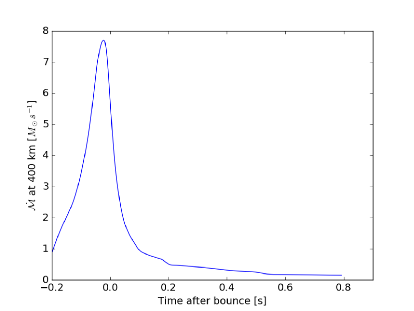
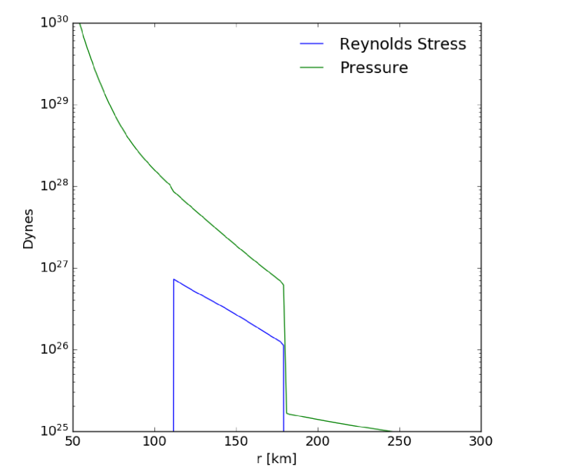
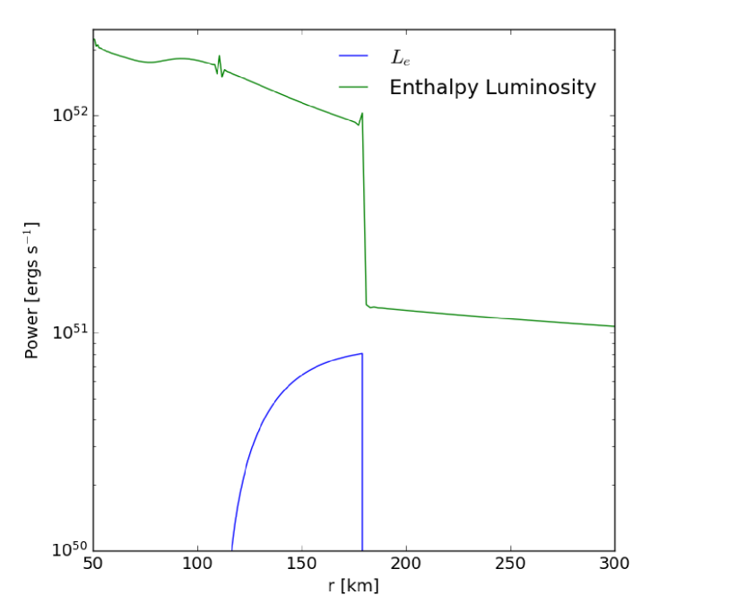
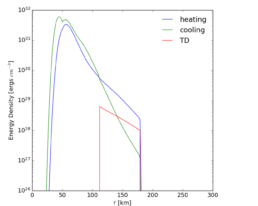
The primary goal is to develop a turbulence model that enables one-dimensional simulations to mimic the evolution, profiles, and explosion conditions of multi-dimensional simulations. First, Figure 1 plots the mass accretion rate vs. time after bounce. Figures 2-4 show the radial profiles, Figures 5 & 6 compare the evolution between 1D+ and 2D, and Figure 7 compares the explosion condition. In this section, we also discuss the implications for future projects.

The mass accretion rate plotted in Figure 1 is an important parameter of the problem, establishing the ram pressure at the shock and the location of the shock. Two important regions to note are roughly at 0.2 s and 0.5 s. The accretion rate drops dramatically due to significant entropy changes in the progenitor’s profile at the boundaries of prior shell burning phases. In general, the mass accretion rate is similar for all progenitors, but the details differ. See Vartanyan et al. (2019) and Ott et al. (2018) for example profiles. The magnitude of accretion rate will differ, and the timing of the drops will differ (c.f. 5 for a zoom-in of this region). The structure of this profile is unique to this specific progenitor, and the explosion outcome is sensitive to this structure. Hence, a primary motivation for the development of the 1D+ technique is to be able to probe the explodability of several progenitors with expedited numerics.

Figure 2 compares profiles of the turbulent correlations with the background. The top panel of Figure 2 shows that the Reynolds stress is a significant fraction (15%) of the pressure within the gain region. Similarly, the turbulent luminosity (middle panel) is roughly 10% of the enthalpy luminosity at the shock. The bottom panel compares turbulent dissipation with neutrino heating and cooling. The ratio of turbulent heating to neutrino heating varies from 10% near the gain radius to 50% near the shock. Note, that the turbulent dissipation plotted in Figure 2 is $\rho\epsilon$, where $\epsilon=R_{rr}^{3/2}/\mathcal{L}$. Even though we assume $R_{rr}$ and $epsilon$ to be constant with radius, the $\rho\epsilon$ is not constant only because of the density profile. The combined effects of turbulent ram pressure, turbulent transport, and, most importantly, turbulent dissipation are crucial in achieving explosion with similar conditions as multi-dimensional simulations.

Figures 3-6, show how these turbulent terms affect the radial profiles. Figure 3 shows the entropy profiles at 350 ms after bounce for the 1D, 1D+, and 2D simulations. In general, the 1D+ simulation mimics the two-dimensional simulation and differs from the one-dimensional simulation in a couple of ways. First, the peak entropy is higher for both the two-dimensional and 1D+ cases. In the 1D+ simulation, this higher entropy is due to turbulent dissipation, and presumably this is the case for the two-dimensional simulation. Second, both the two-dimensional and the 1D+ models show similar entropy profiles in the inner convective region between 15 and 55 km. As designed (see eq. (2.3), the entropy gradient is flat for the inner convection. One difference is that the average shock radius of the 1D+ simulation has a larger radius than the 1D or 2D simulation. The lack of a well-defined shock in the two-dimensional case is a result of an angle-averaged entropy profile; since the shock is not spherically symmetric, the shock is at different radii for different angles. The largest shock radii in the 2D case are similar to the 1D+ shock radius.

Figure 4 shows the resulting changes in the density (top panel) and temperature (bottom) profiles at 350 ms post bounce. Both the density and temperature profiles are shallower as a result of convection (figure 4). This is consistent with the differences seen in steady-state explorations (Mabanta & Murphy, 2018).

Figure 3: Entropy profiles of a one-dimensional, two-dimensional, and 1D+ model. In general, the 1D+ simulation mimics the two-dimensional simulation and differs from the one-dimensional simulation in several ways. Most notably, the entropy is higher for both the 1D+ and two-dimensional simulations. In the 1D+ simulation, this is due to the turbulent dissipation term, which presumably causes the higher entropy in the two-dimensional simulation as well. The 1D+ shock radius is somewhat larger than the average shock radius for the 2D simulation. This may provide a way to more accurately calibrate the convection model with future three-dimensional simulations.

Figure 4: One-dimensional density and temperature profiles with and without the turbulence model. Though the changes are subtle, two important differences are the farther shock radius in the 1D+ case, and the shallower density gradient. Murphy & Dolence (2017); Mabanta & Murphy (2018) note that a shallower post-shock density gradient leads to an ease of explosion.

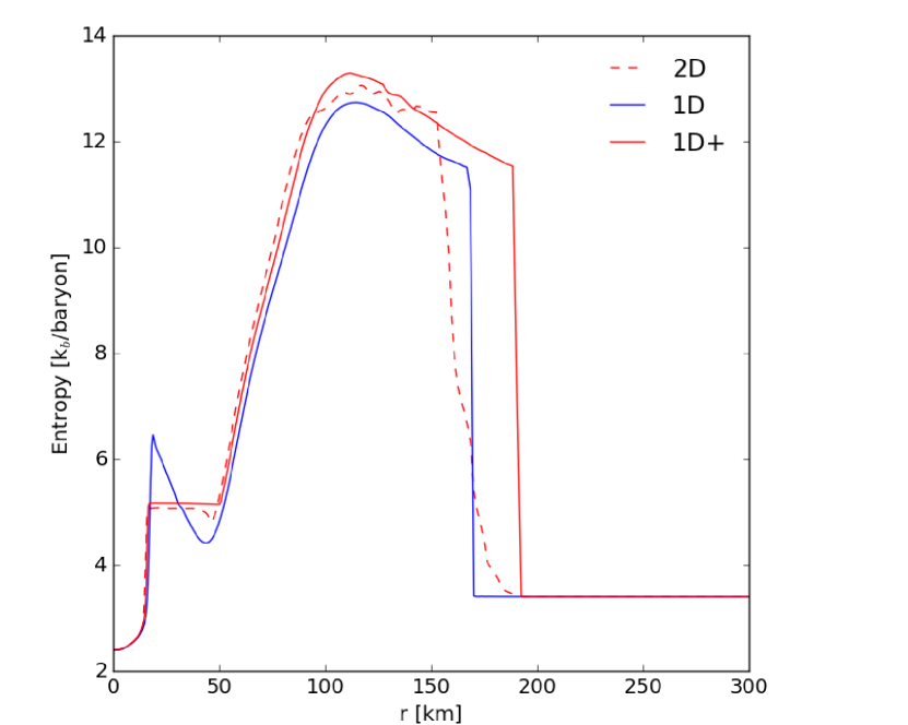
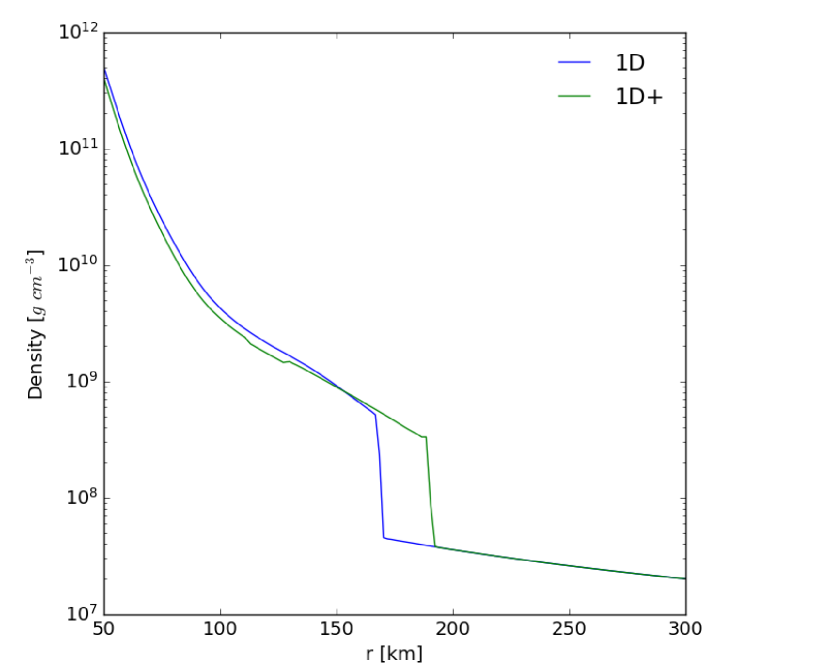
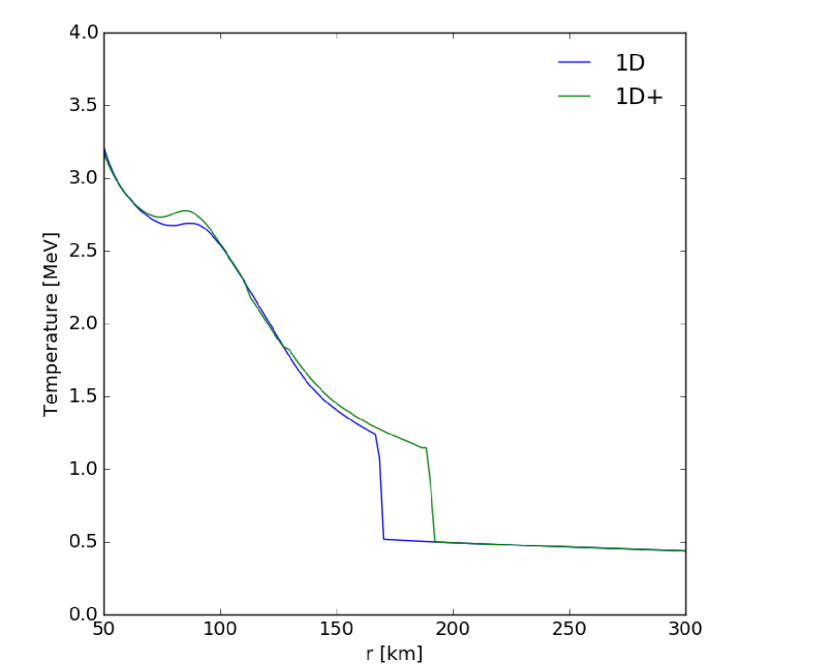
Figure 5 illustrates the shock radius evolution for various neutrino luminosities. For perspective, the blue-dotted line shows the corresponding evolution of $\dot{\mathcal{M}}$ at 400 km, since we declare explosion once the shock exceeds 400 km. This is far enough from the range of oscillations, and hence, explosion is unambiguous. Though this is an arbitrary point, this range is a common, fiducial criterion for explosion (e.g. Sukhbold et al. (2016) uses 500 km). In fact, for these simplified models, past 400km, the shock radius never returns. To determine the $\dot{\mathcal{M}}$ associated with explosion, one can compare the time at which a specific curve crosses 400 km and match that point to its associated $\dot{\mathcal{M}}$ value. Note that many of the high luminosity runs explode at or just after the significant drop at $\sim$0.2 s. This pile-up of explosion times and nearly vertical $\dot{\mathcal{M}}$ vs. time profile makes it difficult to assess a unique explosion time or $\dot{\mathcal{M}}$. For clear comparisons, subsequent analyses focus on the range of luminosities that give explosion after this drop. Finding an (L_ν,$\dot{\mathcal{M}}$) data point where there is a smooth mass accretion rate curve more accurately describes the explosion condition. Figure 6 shows a subset of these shock radii for the 1D+ runs, but this time, the figure also includes shock radii of the two-dimensional simulations. The higher luminosities in this plot have been pruned for clarity. These results show that the 1D+ model explodes at similar times, but slightly earlier than their two-dimensional counterparts.

Figure 5: Shock radius vs. time after bounce for the 1D+ simulations. Each curve is labeled by the neutrino luminosity in units of $10^{52}$ erg s^-1. For reference, the dotted-blue line and the right horizontal axis show the mass accretion rate ($\dot{\mathcal{M}}$). For each model, we note the time of explosion, the corresponding accretion rate, and mark the point (L_ν,$\dot{\mathcal{M}}$) in the critical curve of Figure 7. We define explosion as the point where the shock exceeds 400 km

Figure 6: Shock radius vs. time after bounce for two-dimensional and 1D+ simulations. Again, the label indicates the neutrino luminosity in units of $10^{52}$ erg s^-1. For the most part, the 1D+ and 2D models explode at similar times; the 1D+ models explode slightly earlier, but this makes little difference in the critical curves in Figure 7. To obtain better agreement, one might further tune the turbulence model.

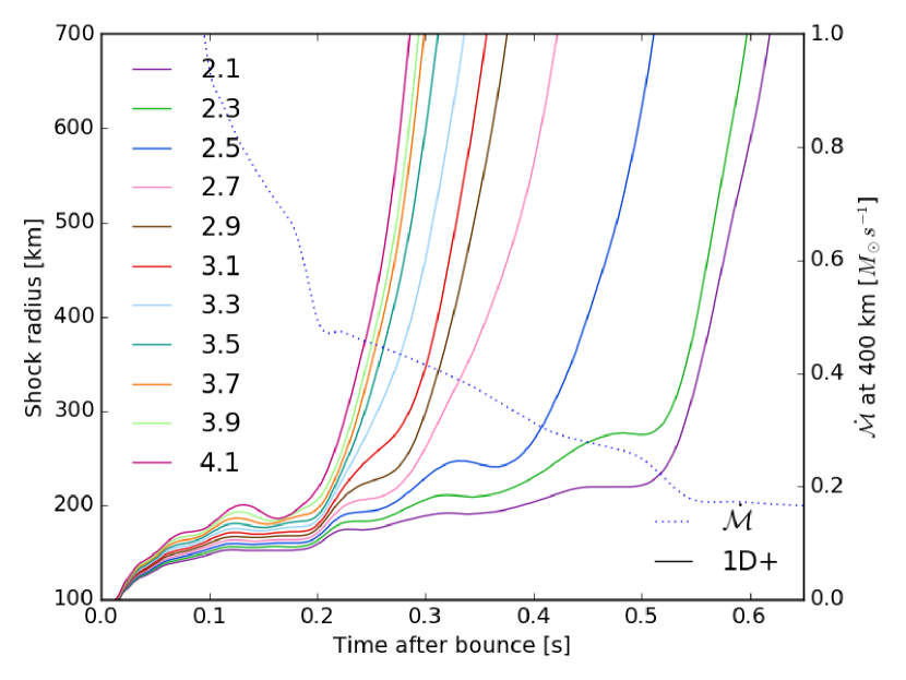
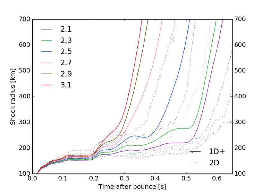
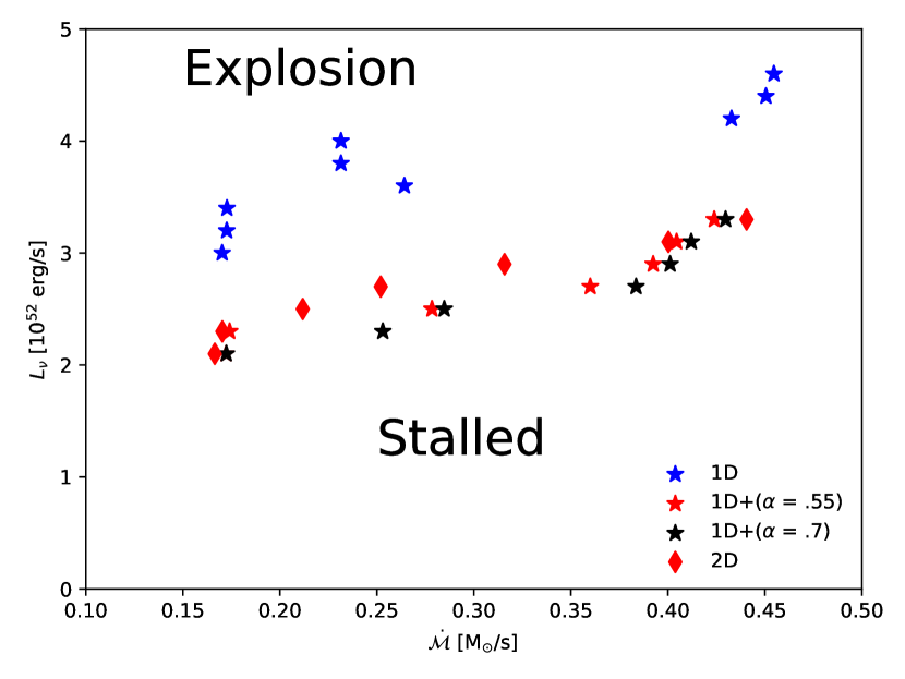
Figure 7 compares the critical luminosities for one-dimensional, 1D+, and two-dimensional simulations. In general, the explosion condition depends upon $L_{\nu}$, $\dot{\mathcal{M}}$, $R_{\text{NS}}$, and $M_{\text{NS}}$ (Murphy & Dolence, 2017). In these simplified models, it is most straightforward to note the luminosity and accretion rate at explosion, so we merely show the $L_{\nu}$-$\dot{\mathcal{M}}$ slice of the critical condition. Here, the blue stars represent explosions in one dimension, the red diamonds represent explosions in two dimensions, and the red and black stars are explosions in our one-dimensional convective model with $\alpha$ = .55 and $\alpha$ = .7, respectively. Note that the reduction between 1D and multi-D (2D in this case) is about 30%, which agrees with the results of other simulations (Murphy & Burrows, 2008; Hanke et al., 2012; Couch, 2013). The 1D+ simulations mimic the critical condition of the 2D simulations, but the 1D+ simulations used a factor of 100 fewer computing resources. If 1D+ simulations also reproduce the explosion conditions of three-dimensional simulations, then the 1D+ simulations could use a factor 100,000 fewer computing resources to predict which stars will explode.

Figure 7: An empirical slice of the condition for explosion: the neutrino-luminosity and accretion-rate critical curve. As has been noted in other simulations, the two-dimensional case requires $\sim$ 30% less neutrino luminosity to explode than the one-dimensional case. The 1D+ critical curve mimics the explosion conditions of 2D simulations. The convection model has two parameters; $\alpha$ relates the neutrino power to turbulent dissipation, and $\beta$ relates the neutrino power to the turbulent luminosity. Two- and three-dimensional simulations show that $\beta=0.3$, but $\alpha$ is different: $\alpha=0.7$ for 3D, and $\alpha=0.55$ for 2D. We test the explodability for both $\alpha$ values and found little difference. For some cases, the turbulence model in this 1D+ simulation is slightly more explosive than the two-dimensional case. Further calibration of the turbulence model might reduce this slight discrepancy.

4 Conclusion

In general, spherically symmetric CCSN simulations often fail to explode while multi-dimensional simulations sometimes do explode. However, these multi-dimensional simulations are very computationally expensive. For example, a recent three-dimensional simulation which ended in a successful explosion required 18 million CPU-hours on 16,000 cores; this one simulation took 1.5 months to compute, and it is one of the most efficient 3D simulations to date (Vartanyan et al., 2019). Sukhbold et al. (2018) noted that the progenitor structure shows significant variation for a small range of masses, and this was for one set of stellar evolution parameters. It may require thousands of CCSN simulations to predict which stars will explode and which won’t. At this rate, it would take hundreds of years to simulate enough progenitors to produce a statistically significant data set. We present a method to incorporate neutrino-driven convection into one-dimensional simulations. These augmented simulations are called 1D+, and they mostly reproduce the profiles and explosion conditions of simple two-dimensional simulations.

The 1D+ simulations include a neutrino-driven convection model that was derived using Reynolds Decomposition (Murphy & Meakin, 2011a; Murphy et al., 2013; Mabanta & Murphy, 2018). It includes Reynolds stress in the momentum equation, turbulent flux in the energy equation, and turbulent dissipation in the energy equation. Two and three dimensional models were used to calibrate the neutrino-driven convection model using three-dimensional simulations with simple neutrino heating and cooling (Murphy et al., 2013). Mabanta & Murphy (2018) included these terms in the steady-state equations describing the stalled shock. They found that the turbulence reproduces the reduction in the critical condition for explosion seen in multi-dimensional simulations. What is more, they found that turbulent dissipation is a dominant effect in this reduction. The 1D+ simulations of this manuscript uses the same neutrino-driven convection model, but here we reformulate the model for time-dependent one-dimensional simulations. These particular 1D+ simulations use a simple neutrino heating and cooling prescription, but the model may work just as well for more sophisticated neutrino transport.

Qualitatively, the 1D+ model reproduces the radial profiles and explosion conditions of simple two-dimensional models. Furthermore, we show how the turbulent terms influence the radial profiles. We have also included the evolution of shock radii for both our 1D+ model and the two-dimensional runs at relevant luminosities. Lastly, we have shown that this technique accurately emulates the luminosity reduction for a successful explosion seen previously in multi-dimensional simulations.

Though 1D+ successfully mimics the explosion condition and profiles of multi-dimensional simulations before explosion, there are several details that the 1D+ model may not replicate. For one, the explosion seems to be inherently aspherical. Simulators noticed that 3-dimensional simulations seem to be dominated by one large buoyant plume (Dolence et al., 2013; Lentz et al., 2015; Müller et al., 2018; Vartanyan et al., 2019). So, while a spherically averaged mean-field convection model seems to reproduce the multidimensional instabilities before explosion, it may not be possible to mimic how explosion develops in a 1D+ model. If true, with the current version of 1D+, this would limit the reliability of post explosion diagnostics such as explosion energy, neutron star masses, nucleosynthetic yields, etc. Going forward, we will compare these post explosion diagnostics with three-dimensional simulations; one may be able to develop mean field models that reflect the multi-dimensional post explosion instabilities. However, since 1D+ is only calibrated to reproduce the explosion conditions of multi-dimensional simulations, our primary focus will be to use 1D+ to predict which stars explode by the neutrino and convection mechanism.

Thus far, the current implementation of 1D+ is consistent with two-dimensional simulations using simple neutrino heating and cooling and Newtonian gravity. The eventual goal is to reproduce the explosion conditions of relativistic three-dimensional radiation-hydrodynamic simulations of CCSNe. The current turbulence model has been calibrated for only a handful of two- and three-dimensional simulations (Murphy & Meakin, 2011a; Murphy et al., 2013). More simulations are necessary to validate the turbulence model in the wide range of conditions seen in core collapse simulations. For example, the neutrino transport of this manuscript is too simple for predictions of explosion; such simulations will require validation with a more nuanced neutrino transport scheme such as two-moment closures (Roberts et al., 2016; Just et al., 2018; O’Connor & Couch, 2018; Skinner et al., 2018; Vartanyan et al., 2019). Furthermore, the turbulence model has only been calibrated with Newtonian monopole gravity. A full validation will require comparisons using non-spherical general relativity. Finally, the turbulence model and explosion conditions have only been validated using a limited set of progenitors. A study considering a wider range of structures and accretion rate histories would help to validate the 1D+ algorithm in the full context of core collapse.

5 Acknowledgments

Quintin A. Mabanta and Joshua C. Dolence acknowledge support from the Laboratory Directed Research and Development Program at Los Alamos National Laboratory. This research used resources provided by the Los Alamos National Laboratory Institutional Computing Program, which is supported by the U.S. Department of Energy National Nuclear Security Administration under Contract No. 89233218CNA000001. This work has been assigned an LANL document release number LA-UR-19-20695. Support for this work was also in part funded by the National Science Foundation under Grant No. 1313036.

References

- Abdikamalov et al. (2016) Abdikamalov, E., Zhaksylykov, A., Radice, D., & Berdibek, S. 2016, ArXiv e-prints, arXiv:1605.09015
- Abdikamalov et al. (2015) Abdikamalov, E., Ott, C. D., Radice, D., et al. 2015, ApJ, 808, 70
- Armstrong et al. (1995) Armstrong, J. W., Rickett, B. J., & Spangler, S. R. 1995, ApJ, 443, 209
- Bethe (1990) Bethe, H. A. 1990, Reviews of Modern Physics, 62, 801
- Bethe & Wilson (1985) Bethe, H. A., & Wilson, J. R. 1985, ApJ, 295, 14
- Blondin et al. (2003) Blondin, J. M., Mezzacappa, A., & DeMarino, C. 2003, ApJ, 584, 971
- Bruenn et al. (2016) Bruenn, S. W., Lentz, E. J., Hix, W. R., et al. 2016, ApJ, 818, 123
- Buras et al. (2006a) Buras, R., Janka, H.-T., Rampp, M., & Kifonidis, K. 2006a, A&A, 457, 281
- Buras et al. (2006b) —. 2006b, A&A, 457, 281
- Buras et al. (2003) Buras, R., Rampp, M., Janka, H.-T., & Kifonidis, K. 2003, Physical Review Letters, 90, 241101
- Burrows & Lattimer (1988) Burrows, A., & Lattimer, J. M. 1988, Phys. Rep., 163, 51
- Burrows et al. (2007) Burrows, A., Dessart, L., Ott, C. D., & Livne, E. 2007, Phys. Rep., 442, 23
- Burrows et al. (2012) Burrows, A., Dolence, J. C., & Murphy, J. W. 2012, ApJ, 759, 5
- Burrows & Goshy (1993) Burrows, A., & Goshy, J. 1993, ApJ, 416, L75
- Burrows et al. (1995) Burrows, A., Hayes, J., & Fryxell, B. A. 1995, ApJ, 450, 830
- Burrows et al. (2016) Burrows, A., Vartanyan, D., Dolence, J. C., Skinner, M. A., & Radice, D. 2016, ArXiv e-prints, arXiv:1611.05859
- Burrows et al. (2018) Burrows, A., Vartanyan, D., Dolence, J. C., Skinner, M. A., & Radice, D. 2018, Space Sci. Rev., 214, 33
- Canuto (1993) Canuto, V. M. 1993, ApJ, 416, 331
- Colgate & Herant (2004) Colgate, S. A., & Herant, M. E. 2004, in Cosmic explosions in three dimensions, ed. P. Höflich, P. Kumar, & J. C. Wheeler, 199
- Couch (2013) Couch, S. M. 2013, ApJ, 775, 35
- Couch & O’Connor (2014) Couch, S. M., & O’Connor, E. P. 2014, ApJ, 785, 123
- Couch & Ott (2015) Couch, S. M., & Ott, C. D. 2015, ApJ, 799, 5
- Dolence et al. (2013) Dolence, J. C., Burrows, A., Murphy, J. W., & Nordhaus, J. 2013, ApJ, 765, 110
- Dolence et al. (2015) Dolence, J. C., Burrows, A., & Zhang, W. 2015, ApJ, 800, 10
- Ertl et al. (2016) Ertl, T., Janka, H.-T., Woosley, S. E., Sukhbold, T., & Ugliano, M. 2016, ApJ, 818, 124
- Fernández (2015a) Fernández, R. 2015a, MNRAS, 452, 2071
- Fernández (2015b) —. 2015b, MNRAS, 452, 2071
- Fernández et al. (2014) Fernández, R., Müller, B., Foglizzo, T., & Janka, H.-T. 2014, MNRAS, 440, 2763
- Foglizzo et al. (2006) Foglizzo, T., Scheck, L., & Janka, H.-T. 2006, ApJ, 652, 1436
- Foglizzo & Tagger (2000) Foglizzo, T., & Tagger, M. 2000, A&A, 363, 174
- Foglizzo et al. (2015) Foglizzo, T., Kazeroni, R., Guilet, J., et al. 2015, PASA, 32, e009
- Fryer (1999) Fryer, C. L. 1999, ApJ, 522, 413
- Guilet et al. (2010) Guilet, J., Sato, J., & Foglizzo, T. 2010, ApJ, 713, 1350
- Handy et al. (2014) Handy, T., Plewa, T., & Odrzywołek, A. 2014, ApJ, 783, 125
- Hanke et al. (2012) Hanke, F., Marek, A., Müller, B., & Janka, H.-T. 2012, ApJ, 755, 138
- Hanke et al. (2013) Hanke, F., Müller, B., Wongwathanarat, A., Marek, A., & Janka, H.-T. 2013, ApJ, 770, 66
- Steiner et al. (2013) Steiner, A. W., Hempel, M., & Fischer, T. 2013, ApJ, 774, 17
- Herant et al. (1994) Herant, M., Benz, W., Hix, W. R., Fryer, C. L., & Colgate, S. A. 1994, ApJ, 435, 339
- Hillebrandt & Mueller (1981) Hillebrandt, W., & Mueller, E. 1981, A&A, 103, 147
- Horiuchi et al. (2011) Horiuchi, S., Beacom, J. F., Kochanek, C. S., et al. 2011, ApJ, 738, 154
- Iwakami et al. (2014) Iwakami, W., Nagakura, H., & Yamada, S. 2014, ApJ, 793, 5
- Janka (2001) Janka, H.-T. 2001, A&A, 368, 527
- Janka et al. (2007) Janka, H.-T., Langanke, K., Marek, A., Martínez-Pinedo, G., & Müller, B. 2007, Phys. Rep., 442, 38
- Janka (2017) —. 2017, ArXiv e-prints, arXiv:1702.08825
- Janka & Keil (1998) Janka, H.-T., & Keil, W. 1998, in Supernovae and cosmology, ed. L. Labhardt, B. Binggeli, & R. Buser, 7
- Janka et al. (2016) Janka, H.-T., Melson, T., & Summa, A. 2016, ArXiv e-prints, arXiv:1602.05576
- Janka & Müller (1995) Janka, H.-T., & Müller, E. 1995, ApJ, 448, L109
- Janka & Müller (1996) —. 1996, A&A, 306, 167
- Just et al. (2018) Just, O., Bollig, R., Janka, H.-T., et al. 2018, MNRAS, 481, 4786
- Kitaura et al. (2006) Kitaura, F. S., Janka, H.-T., & Hillebrandt, W. 2006, A&A, 450, 345
- Kolmogorov (1941) Kolmogorov, A. 1941, Akademiia Nauk SSSR Doklady, 30, 301
- Lentz et al. (2015) Lentz, E. J., Bruenn, S. W., Hix, W. R., et al. 2015, ArXiv e-prints, arXiv:1505.05110
- Li et al. (2011) Li, W., Leaman, J., Chornock, R., et al. 2011, MNRAS, 412, 1441
- Liebendörfer et al. (2001a) Liebendörfer, M., Mezzacappa, A., & Thielemann, F.-K. 2001a, Phys. Rev. D, 63, 104003
- Liebendörfer et al. (2001b) Liebendörfer, M., Mezzacappa, A., Thielemann, F.-K., et al. 2001b, Phys. Rev. D, 63, 103004
- Liebendörfer et al. (2005) Liebendörfer, M., Rampp, M., Janka, H.-T., & Mezzacappa, A. 2005, ApJ, 620, 840
- Mabanta & Murphy (2018) Mabanta, Q. A., & Murphy, J. W. 2018, ApJ, 856, 22
- Marek & Janka (2009) Marek, A., & Janka, H.-T. 2009, ApJ, 694, 664
- Mazurek (1982) Mazurek, T. J. 1982, ApJ, 259, L13
- Mazurek et al. (1982) Mazurek, T. J., Cooperstein, J., & Kahana, S. 1982, in NATO Advanced Science Institutes (ASI) Series C, Vol. 90, NATO Advanced Science Institutes (ASI) Series C, ed. M. J. Rees & R. J. Stoneham, 71–77
- Meakin & Arnett (2007) Meakin, C. A., & Arnett, D. 2007, ApJ, 667, 448
- Meakin & Arnett (2010) Meakin, C. A., & Arnett, W. D. 2010, Ap&SS, 328, 221
- Perego et al. (2015) Perego, A., Hempel, M., Fröhlich, C., et al. 2015, ApJ, 806, 275
- Melson et al. (2015) Melson, T., Janka, H.-T., & Marek, A. 2015, ApJ, 801, L24
- Müller (2016) Müller, B. 2016, ArXiv e-prints, arXiv:1608.03274
- Müller (2017) —. 2017, ArXiv e-prints, arXiv:1702.06940
- Müller et al. (2016) Müller, B., Heger, A., Liptai, D., & Cameron, J. B. 2016, MNRAS, 460, 742
- Müller et al. (2017) Müller, B., Melson, T., Heger, A., & Janka, H.-T. 2017, ArXiv e-prints, arXiv:1705.00620
- Müller et al. (2018) Müller, B., Tauris, T. M., Heger, A., et al. 2018, arXiv:1811.05483
- Murphy & Burrows (2008) Murphy, J. W., & Burrows, A. 2008, ApJ, 688, 1159
- Murphy & Dolence (2017) Murphy, J. W., & Dolence, J. C. 2017, ApJ, 834, 183
- Murphy et al. (2013) Murphy, J. W., Dolence, J. C., & Burrows, A. 2013, ApJ, 771, 52
- Murphy & Meakin (2011a) Murphy, J. W., & Meakin, C. 2011a, ApJ, 742, 74
- Murphy & Meakin (2011b) —. 2011b, ApJ, 742, 74
- O’Connor & Ott (2011) O’Connor, E., & Ott, C. D. 2011, ApJ, 730, 70
- O’Connor et al. (2017) O’Connor, E., Horowitz, C. J., Lin, Z., & Couch, S. 2017, Supernova 1987A:30 years later - Cosmic Rays and Nuclei from Supernovae and their Aftermaths, 331, 107
- Ott et al. (2013) Ott, C. D., Abdikamalov, E., Mösta, P., et al. 2013, ApJ, 768, 115
- Ott et al. (2018) Ott, C. D., Roberts, L. F., da Silva Schneider, A., et al. 2018, ApJ, 855, L3
- O’Connor & Couch (2018) O’Connor, E. P., & Couch, S. M. 2018, ApJ, 865, 81
- Pejcha & Thompson (2012) Pejcha, O., & Thompson, T. A. 2012, ApJ, 746, 106
- Pejcha & Thompson (2015) Pejcha, O., & Thompson, T. A. 2015, ApJ, 801, 90
- Radice et al. (2017) Radice, D., Burrows, A., Vartanyan, D., Skinner, M. A., & Dolence, J. C. 2017, ArXiv e-prints, arXiv:1702.03927
- Radice et al. (2016) Radice, D., Ott, C. D., Abdikamalov, E., et al. 2016, ApJ, 820, 76
- Rampp & Janka (2002) Rampp, M., & Janka, H.-T. 2002, A&A, 396, 361
- Roberts et al. (2016) Roberts, L. F., Ott, C. D., Haas, R., et al. 2016, ArXiv e-prints, arXiv:1604.07848
- Sato et al. (2009a) Sato, J., Foglizzo, T., & Fromang, S. 2009a, ApJ, 694, 833
- Sato et al. (2009b) Sato, J., Foglizzo, T., & Fromang, S. 2009b, in SF2A-2009: Proceedings of the Annual meeting of the French Society of Astronomy and Astrophysics, ed. M. Heydari-Malayeri, C. Reyl’E, & R. Samadi, 175
- Sinha et al. (2017) Sinha, S., Ebinger, K., Frohlich, C., et al. 2017, APS Meeting Abstracts, J12.007
- Skinner et al. (2018) Skinner, M. A., Dolence, J. C., Burrows, A., Radice, D., & Vartanyan, D. 2018, arXiv:1806.07390
- Sukhbold et al. (2016) Sukhbold, T., Ertl, T., Woosley, S. E., Brown, J. M., & Janka, H.-T. 2016, ApJ, 821, 38
- Sukhbold et al. (2018) Sukhbold, T., Woosley, S. E., & Heger, A. 2018, ApJ, 860, 93
- Tamborra et al. (2017) Tamborra, I., Hüdepohl, L., Raffelt, G. G., & Janka, H.-T. 2017, ApJ, 839, 132
- Thompson (2000) Thompson, C. 2000, ApJ, 534, 915
- Thompson et al. (2003) Thompson, T. A., Burrows, A., & Pinto, P. A. 2003, ApJ, 592, 434
- Thompson et al. (2005) Thompson, T. A., Quataert, E., & Burrows, A. 2005, ApJ, 620, 861
- Ugliano et al. (2012) Ugliano, M., Janka, H.-T., Marek, A., & Arcones, A. 2012, ApJ, 757, 69
- Vartanyan et al. (2019) Vartanyan, D., Burrows, A., Radice, D., Skinner, M. A., & Dolence, J. 2019, MNRAS, 477, 3091
- Woosley & Heger (2007) Woosley, S. E., & Heger, A. 2007, Phys. Rep., 442, 269
- Yamasaki & Yamada (2005) Yamasaki, T., & Yamada, S. 2005, ApJ, 623, 1000
- Yamasaki & Yamada (2006) —. 2006, ApJ, 650, 291