NETT Regularization for Compressed Sensing Photoacoustic Tomography

Abstract

We discuss several methods for image reconstruction in compressed sensing photoacoustic tomography (CS-PAT). In particular, we apply the deep learning method of [H. Li, J. Schwab, S. Antholzer, and M. Haltmeier. NETT: Solving Inverse Problems with Deep Neural Networks (2018), arXiv:1803.00092], which is based on a learned regularizer, for the first time to the CS-PAT problem. We propose a network architecture and training strategy for the NETT that we expect to be useful for other inverse problems as well. All algorithms are compared and evaluated on simulated data, and validated using experimental data for two different types of phantoms. The results on the one the hand indicate great potential of deep learning methods, and on the other hand show that significant future work is required to improve their performance on real-word data.

Keywords: Compressed sensing, photoacoustic tomography, deep learning, NETT, learned regularizer, Tikhonov regularization, $\ell^{1}$-regularization, neural networks, inverse problems

1 Introduction

Compressed Sensing (CS) is a promising tool to reduce the number spatial measurements in photoacoustic tomography (PAT), while still keeping good image quality. Reducing the number of measurements can be used to lower system costs, to speed up data acquisition, and to reduce motion artifacts [1, 2, 3]. In this work, we concentrate on 2D PAT, which arises in PAT with integration line detectors [4, 5]. If one can use enough sensor locations such that Shannon’s sampling theory is applicable, it is possible to get high resolution images using analytic inversion methods [6]. In practice, however, the number of measurements is much lower than required for high resolution images according to Shannon’s sampling theory. In such a situation, standard reconstruction methods result in undersampling artifacts and low resolution images.

To accelerate the data acquisition process, systems with 64 line detectors have been built [7, 8]. Such systems offer the possibility to collect 2D photoacoustic (PA) projection images of the 3D source images at a frame-rate of $20\text{\,}\mathrm{Hz}$ or higher [9]. Using 64 spatial sampling positions still results in highly under-sampled data. In order to get high resolution reconstructions from such data, one has to exploit additional information available on the PA source images. In [10], the sparsity of the Laplacian is used in combination with $\ell_{1}$-minimization. Recently, machine learning methods have been applied to CS-PAT [11]. In this work, we develop several machine learning methods for CS-PAT and apply them to experimental CS-PAT data. Comparison with joint $\ell_{1}$-minimization is also given.

In contrast to [11], we also implement the NETT [12], which uses a neural network as trained regularizer for CS-PAT image reconstruction. In particular, we propose a simpler network architecture and training strategy than the one used in [12]. The proposed strategy for the regularizer in NETT may be useful for other inverse problems as well.

2 Background

In this section we describe the CS-PAT problem, and present the joint $\ell^{1}$-algorithm as well as the standard deep learning approach for CS-PAT image reconstruction. The NETT will be introduced in Section 3.

2.1 Compressed sensing PAT

PAT relies on the following principle. When an object of interest is illuminated with a short laser pulse, an acoustic pressure wave is induced inside the object. This pressure wave is recorded on the outside of the object and used for reconstructing an image of the interior. In the following we will restrict ourselves to the 2D case in a circular measurement geometry, which arises when using integrating line detectors [4, 5].

Let $p_{0}\colon\mathbb{R}^{2}\to\mathbb{R}$ denote the PA source (initial pressure distribution). The induced pressure wave satisfies the following equation

$$\partial^{2}p(\mathbf{r},t)-c^{2}\Delta_{\mathbf{r}}p(\mathbf{r},t)=\delta^{\prime}(t)p_{0}(\mathbf{r})\quad\text{for }(\mathbf{r},t)\in\mathbb{R}^{2}\times\mathbb{R}_{+}\,,$$ (1)

where $\mathbf{r}\in\mathbb{R}^{2}$ is the spatial location, $t\in\mathbb{R}_{+}$ the time variable, $\Delta_{\mathbf{r}}$ the spatial Laplacian, and $c$ is the speed of sound. We further assume that the PA source $p_{0}(\mathbf{r})$ vanishes outside the disc $B_{R}=\{\mathbf{x}\in\mathbb{R}^{2}\mid\lVert\mathbf{x}\rVert<R\}$ and we set $p(\mathbf{r},t)=0$ for $t<0$. Then $p(\mathbf{r},t)$ is uniquely defined and we refer to it as the causal solution of (1).

The PAT problem consists in recovering $p_{0}(\mathbf{r})$ from measurements of $p(\mathbf{s},t)$ on $\partial B_{R}\times(0,\infty)$, where $\mathbf{s}$ stands for the detector location. In the full data case, as shown in [13], the following filtered backprojection formula (FBP) formula yields an exact reconstruction of the PA source,

$$p_{0}(\mathbf{r})=-\frac{1}{\pi R}\int_{\partial B_{R}}\!{\int_{\lvert\mathbf{r}-z\rvert}^{\infty}\!{\frac{(\partial_{t}tp)(\mathbf{s},t)}{\sqrt{t^{2}-\lvert\mathbf{r}-\mathbf{s}\rvert^{2}}}}\,\mathrm{d}{t}}\,\mathrm{d}{S(\mathbf{s})}\,.$$ (2)

Additionally, in [13] it was shown that the operator defined by the right hand side of (2) is the adjoint of the forward operator of the wave equation.

In practical application, the pressure can only be measured with a finite number of samples. This means we measure data

$$p(\mathbf{s}_{k},t_{l})\text{ for }(k,l)\in\{1,\ldots,M\}\times\{1,\ldots,Q\}\,,$$ (3)

where the sampling points are uniformly sampled, i.e.

$$\mathbf{s}_{k}=\left[\begin{array}[]{c}R\cos(2\pi(k-1)/M)\\ R\sin(2\pi(k-1)/M)\end{array}\right]\quad t_{l}=2R(l-1)/(Q-1)\,.$$ (4)

As shown in [6], using classical Shannon sampling theory, the number $M$ of spatial measurements in (3), (4) determines the resolution of the reconstructed PA source. To reduce the number of measurements while preserving high resolution we apply CS. Instead of collecting $M$ samples, we measure generalized samples

$$\mathbf{g}(j,l)=\sum_{k=1}^{M}\mathbf{S}[j,k]p(\mathbf{r}_{k},t_{l})\quad\text{for }j\in\{1,\ldots,m\}\,,$$ (5)

with $m\ll M$. Several choices of the sampling matrix $\mathbf{S}$ exist [1, 2, 3]. In this work we will focus on two cases, namely a deterministic subsampling matrix and a random Bernoulli matrix.

Let us denote the discretized solution operator of the wave equation by $\mathcal{W}\in\mathbb{R}^{MQ\times n}$, were $n$ is the discretization size of the reconstruction, and by $\mathcal{S}=\mathbf{S}\otimes\mathbf{I}\in\mathbb{R}^{mQ\times MQ}$ the Kronecker product between the CS measurement matrix $\mathbf{S}$ and the identity matrix. If we denote the discrete initial pressure by $\mathbf{x}\in\mathbb{R}^{n}$, we can write the measurement process the following way

$$\mathbf{y}=\mathcal{A}\mathbf{x}+\varepsilon\quad\text{with }\mathcal{A}=\mathcal{S}\circ\mathcal{W}\in\mathbb{R}^{mQ\times n}\,.$$ (6)

Since $mQ\ll n$, equation (6) is under-determined and its solution requires specialized reconstruction algorithms that incorporate additional knowledge about the unknowns. Such algorithms will be described in the following.

2.2 Residual networks

Deep learning has been recently applied to several image reconstruction problems [14, 15, 16] including PAT [11, 17, 18, 19, 20].

Figure 1: Architecture of the residual U-net. The number of convolution kernels (channels) is written over each layer. Long arrows indicate direct connections with subsequent concatenation or addition.

The probably simplest approach is to use an explicit reconstruction function $R_{\theta}=\mathcal{N}_{\theta}\circ\mathcal{A}^{\sharp}\colon\mathbb{R}^{mQ}\to\mathbb{R}^{n}$ where $\mathcal{N}_{\theta}$ is a neural network (NN) and $\mathcal{A}^{\sharp}$ is an operator that performs an initial reconstruction. In order to determine the parameter vector $\theta\in\mathbb{R}^{p}$ (where $p$ can be very large) that parameterizes the NN, one minimizes an error function averaged over a finite set of training data $(\mathbf{b}_{k},\mathbf{f}_{k})_{k=1}^{N}$. Here $\mathbf{f}_{k}$ are samples of phantoms and $\mathbf{b}_{k}=\mathcal{A}^{\sharp}\mathcal{A}(\mathbf{f}_{k})$ the corresponding input images. Then one solves the following optimization problem iteratively

$$\min_{\theta}\frac{1}{N}\sum_{k=1}^{N}\lVert\mathcal{N}_{\theta}(\mathbf{b}_{k})-\mathbf{f}_{k}\rVert_{p}^{q}\,.$$ (7)

In particular, stochastic gradient and variants are frequently applied to approximately minimize (7).

In order to simplify the learning procedure [16], it has been proposed to train a NN that learns the residual images $\mathbf{f}-\mathbf{b}=\mathbf{f}-\mathcal{A}^{\sharp}\mathcal{A}\mathbf{f}$. In such a situation, the reconstruction function has the form

$$R_{\theta}^{\text{res}}=(\operatorname{Id}+\mathcal{U}_{\theta})\mathcal{A}^{\sharp}\,,$$ (8)

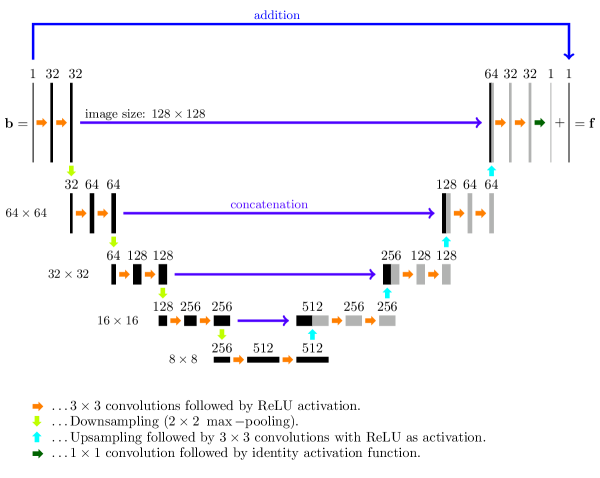
where $\theta\in\mathbb{R}^{p}$ is the adjustable parameter vector. A popular choice [17, 15, 16] for $\mathcal{U}_{\theta}$ is the so called U-net, which was originally designed for image segmentation [21]. The resulting NN architecture is shown in Figure 1. Variants of the residual structure to increase data consistence have been proposed in [22, 23].

2.3 Joint $\ell_{1}$-minimization

In [10] a method based on $\ell_{1}$-minimization was introduced which relies on sparsity. An element $\mathbf{v}\in\mathbb{R}^{n}$ is called $s$-sparse, with $s\in\{1,\dots,n\}$, if it contains at most $s$ nonzero elements. One can reconstruct $\mathbf{v}$ in a stable manner from measurements $\mathbf{g}=\mathcal{A}\mathbf{v}$ provided that $\mathcal{A}$ satisfies the restricted isometry property (RIP) of order $2s$. This property means that $(1-\delta)\lVert\mathbf{z}\rVert^{2}\leq\lVert\mathcal{A}\mathbf{z}\rVert^{2}\leq(1+\delta)\lVert z\rVert^{2}$ holds for all $\mathbf{z}\in\mathbb{R}^{n}$ which are $2s$-sparse and the constant $\delta<1/\sqrt{2}$ [24]. Bernoulli matrices satisfy the RIP with high probability [24], but the subsampling matrix does not. Also it is not clear if the forward operator $\mathcal{A}=(\mathbf{S}\otimes\mathbf{I})\circ\mathcal{W}$ satisfies the RIP for any sampling matrix. However the following result from inverse problems theory can still be applied in this case.[25]

Theorem 1. Let $\mathcal{A}\in\mathbb{R}^{mQ\times n}$ and $\mathbf{v}\in\mathbb{R}^{n}$. Assume that the source condition holds: $\exists\mathbf{w}\in\mathbb{R}^{mQ}\colon\mathcal{A}^{\intercal}\mathbf{w}\in\operatorname{sign}(\mathbf{v})\wedge\forall i\in\mathrm{supp}(\mathbf{v})\colon\lvert(\mathcal{A}^{\intercal}\mathbf{w})_{i}\rvert<1$, where $\operatorname{sign}(\mathbf{v})$ is the set-valued signum function and $\mathrm{supp}(\mathbf{v})$ is the set of indices with nonzero components of $\mathbf{v}$. Further, assume that $\mathcal{A}$, restricted to the subspace spanned by $e_{i}$ for $i\in\mathrm{supp}(\mathbf{v})$, is injective. Then for any $\mathbf{g}^{\delta}\in\mathbb{R}^{mQ}$ such that $\lVert\mathcal{A}\mathbf{v}-\mathbf{g}^{\delta}\rVert_{2}\leq\delta$ and any minimizer of the $\ell_{1}$-Tikhonov functional, $\mathbf{v}_{\lambda}^{\delta}\in\operatorname*{argmin}_{\mathbf{z}}\frac{1}{2}\lVert\mathcal{A}\mathbf{z}-\mathbf{g}^{\delta}\rVert_{2}^{2}+\lambda\lVert\mathbf{z}\rVert_{1}$ we have $\lVert\mathbf{v}_{\lambda}^{\delta}-\mathbf{v}\rVert_{2}=\mathcal{O}(\delta)$ provided that $\lambda\asymp\delta$.

It was also shown [25], that the RIP implies the source condition of Theorem 1. Additionally, a smaller support set $\mathrm{supp}(\mathbf{v})$ makes it easier to fulfill the conditions in Theorem 1. This indicates that sparsity of the unknowns is an important requirement for $\ell_{1}$-minimization. The sparsity approach of [10] is based on the following result: [10] If $f$ is an initial PA source vanishing outside of $B_{R}$ and let $p$ be the causal solution of (1). Then $\partial_{t}^{2}p$ is the causal solution of (1) with modified source, $\partial^{2}q(\mathbf{r},t)-\Delta_{\mathbf{r}}q(\mathbf{r},t)=\delta^{\prime}(t)c^{2}\Delta\mathbf{f}(\mathbf{r})\quad\text{for }(\mathbf{r},t)\in\mathbb{R}^{2}\times\mathbb{R}_{+}$. As a consequence we have that

$$\forall\mathbf{f}\in\mathbb{R}^{n}\colon\quad\mathcal{D}_{t}^{2}\mathcal{A}\mathbf{f}=\mathcal{A}(c^{2}\mathcal{L}_{\mathbf{r}}\mathbf{f})$$ (9)

holds up to discretization errors, where $\mathcal{L}_{\mathbf{r}}$ is the discrete Laplacian and $\mathcal{D}_{t}$ the discrete temporal derivative.

For typical PA sources, $\mathcal{L}_{\mathbf{r}}\mathbf{f}$ is sparse or at least compressible. Thus, based on (9), one could first recover $\mathcal{L}_{\mathbf{r}}$ by solving the following $\ell_{1}$-problem $\operatorname*{argmin}_{\mathbf{z}}\{\lVert\mathbf{z}\rVert_{1}\mid\mathcal{A}\mathbf{z}=\mathcal{D}_{t}^{2}\mathbf{g}\}$, and then solve the Poisson equation $\mathcal{L}_{\mathbf{r}}\mathbf{f}=\mathbf{g}/c^{2}$ with zero boundary conditions in order to get $\mathbf{f}$. However, this approach leads to low frequency artifacts in the reconstructed phantom. To overcome this issue, a joint minimization approach was introduced [10], which jointly reconstructs $\mathbf{f}$ and $\mathbf{\mathcal{L}_{\mathbf{r}}\mathbf{f}}$. In practice, one minimizes the following

$$\min_{\mathbf{f},\mathbf{h}}\frac{1}{2}\lVert\mathcal{A}\mathbf{f}-\mathbf{g}\rVert_{2}^{2}+\frac{1}{2}\lVert\mathcal{A}\mathbf{h}-\mathcal{D}_{t}^{2}\mathbf{g}\rVert_{2}^{2}+\frac{\alpha}{2}\lVert\mathcal{L}_{\mathbf{r}}\mathbf{f}-\mathbf{h}/c^{2}\rVert_{2}^{2}+\beta\lVert\mathbf{h}\rVert_{1}+I_{C}(\mathbf{f})\,,$$ (10)

where $\alpha$ is a tuning parameter and $\beta$ is a regularization parameter. Moreover, $I_{C}$ implements a positivity constraint, i.e. with $C=[0,\infty)^{n}$, the function $I_{C}$ is defined by $I_{C}(\mathbf{f})=0$ if $\mathbf{f}\in C$ and $I_{C}(\mathbf{f})=\infty$ otherwise.

To solve (10), one can use a proximal forward-backward splitting method [26], which is applicable to problems separable into smooth and non-smooth but convex parts. Here we take the smooth part as $\Phi(\mathbf{f},\mathbf{h})=1/2\lVert\mathcal{A}\mathbf{f}-\mathbf{g}\rVert_{2}^{2}+1/2\lVert\mathcal{A}\mathbf{h}-\mathcal{D}_{t}^{2}\mathbf{g}\rVert_{2}^{2}+\alpha/2\lVert\mathcal{L}_{\mathbf{r}}\mathbf{f}-\mathbf{h}/c^{2}\rVert_{2}^{2}$ and the non-smooth part as $\Psi(\mathbf{f},\mathbf{h})=\beta\lVert\mathbf{h}\rVert_{1}+I_{C}(\mathbf{f})$. We need to calculate the proximity operator of the non-smooth parts, which, for a convex function $F\colon\mathbb{R}^{n}\to\mathbb{R}$, is defined by $\operatorname{prox}_{F}(\mathbf{f})\triangleq\operatorname*{argmin}\{F(\mathbf{z})+\tfrac{1}{2}\lVert\mathbf{f}-\mathbf{z}\rVert_{2}^{2}\mid\mathbf{z}\in\mathbb{R}^{n}\}$. In our case, the proximity operator can be computed explicitly and component-wise, $\operatorname{prox}_{\Psi}(\mathbf{f},\mathbf{h})=[\operatorname{prox}_{I_{C}}(\mathbf{f}),\operatorname{prox}_{\beta\lVert\,\cdot\,\rVert_{1}}(\mathbf{h})]$. On the other hand, the gradients of $\Phi$ can also be calculated explicitly. The resulting joint $\ell^{1}$-minimization algorithm for (10) is given by the following iterative scheme

$$\mathbf{f}^{k+1}= \operatorname{prox}_{I_{C}}\left(\mathbf{f}^{k}-\mu\left(\mathcal{A}^{\intercal}(\mathcal{A}\mathbf{f}^{k}-\mathbf{g})-\alpha\mathcal{L}(\mathcal{L}\mathbf{f}^{k}-\mathbf{h}^{k}/c^{2})\right)\right)$$ (11)

$$\mathbf{h}^{k+1}= \operatorname{prox}_{\beta\lVert\,\cdot\,\rVert_{1}}\left(\mathbf{h}^{k}-\mu\left(\mathcal{A}^{\intercal}(\mathcal{A}\mathbf{h}^{k}-\mathcal{D}_{t}^{2}\mathbf{g})-\frac{\alpha}{c^{2}}(\mathcal{L}_{\mathbf{r}}\mathbf{f}^{k}-\mathbf{h}^{k}/c^{2})\right)\right)\,,$$

with starting points $\mathbf{f}^{0}=\mathbf{h}^{0}=\mathbf{0}$ and $\operatorname{prox}_{I_{C}}(\mathbf{f})=(\max(\mathbf{f}_{i},0))_{i}$, $\operatorname{prox}_{\beta\lVert\,\cdot\,\rVert_{1}}(\mathbf{h})=(\max(\lvert\mathbf{h}_{i}\rvert-\beta,0)\operatorname{sign}(\mathbf{h}_{i}))$.

3 Nett: variational regularization with neural networks

Standard deep learning approaches have the disadvantage that they may perform badly on images that are very different from the ones included in the training set. In order to address this issue, iterative networks [27, 28, 29] or data invariant regularizing networks [23] have been proposed. Another method to enhance data consistency, which we will use in this paper, is based on generalized Tikhonov regularization using a learned regularization term [12].

3.1 NETT framework

The basic idea is to consider minimizers of the unconstrained optimization problem

$$\min_{\mathbf{f}}\frac{1}{2}\lVert\mathcal{A}\mathbf{f}-\mathbf{g}\rVert_{2}^{2}+\frac{\lambda}{2}\,\mathcal{R}(\mathbf{f})\,,$$ (12)

where $\mathcal{R}\colon\mathbb{R}^{n}\to[0,\infty]$ is a trained regularizer and $\lambda>0$ is the regularization parameter. The resulting reconstruction approach is called NETT (for network Tikhonov regularization), as it is a generalized form of Tikhonov regularization using a NN as trained regularizer.

In [12] it has been shown that under reasonable conditions, the NETT approach is well-posed and yields a convergent regularization method. In particular, minimizers of (12) exist, are stable with respect to data perturbations, and minimizers of (12) converge to $\mathcal{R}$-minimizing solutions of the equation $\mathcal{A}\mathbf{f}=\mathbf{g}$ as the noise level goes to zero. For the regularizer proposed in [12] these conditions are difficult to be verified. We propose a variation of the trained regularizer using a simpler network architecture and different training strategy.

3.2 Construction of regularizers

For the regularizer in (12) we make the ansatz

$$\mathcal{R}(\mathbf{f})=\lVert\mathcal{V}_{\theta}(\mathbf{f})\rVert_{F}^{2}\,,$$ (13)

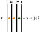
where $\lVert\cdot\rVert_{F}$ is the Frobenius norm and $\mathcal{V}_{\theta}\colon\mathbb{R}^{n}\to\mathbb{R}^{n}$ is a trained NN. In this work, we use the simple NN architecture shown in Figure 2, that consist of three convolutional layers. Clearly, one could also use more complicated network structures.

Figure 2: Network structure for the trained regularizer. The first two convolutional layers use $3\times 3$ convolutions followed by ReLU activations. The last convolutional layer (green arrow) uses $3\times 3$ convolutions not followed by an activation function.

To train the network $\mathcal{V}_{\theta}$ we choose a set of phantoms $(\mathbf{f}_{k})_{k=1}^{N_{1}+N_{2}}$ and compute initial reconstructions $\mathbf{b}_{k}=\mathcal{A}^{\sharp}\mathcal{A}\mathbf{f}_{k}$. We then define a training set of input/output pairs $(\mathbf{x}_{k},\mathbf{y}_{k})_{k=1}^{N_{1}+N_{2}}$ in the following way:

$$\mathbf{x}_{k} =\mathbf{b}_{k}\,, \mathbf{y}_{k}=\mathbf{b}_{k}-\mathbf{f}_{k}\quad \text{for }k =1,\ldots,N_{1}$$ (14)

$$\mathbf{x}_{k} =\mathbf{f}_{k}\,, \mathbf{y}_{k}=\mathbf{0} \text{for }k =N_{1}+1,\ldots,N_{1}+N_{2}\,.$$

The parameters in the network $\mathcal{V}_{\theta}$ are optimized to approximately map $\mathbf{x}_{k}$ to $\mathbf{y}_{k}$. For that purpose we minimize the mean absolute error

$$E(\theta)=\frac{1}{N_{1}+N_{2}}\sum_{k=1}^{N_{1}+N_{2}}\lVert\mathcal{V}_{\theta}(\mathbf{x}_{k})-\mathbf{y}_{k}\rVert_{1}\,.$$ (15)

averaged of the training set.

Note that the trained regularizer depends on the forward operator as well as on the initial reconstruction operator. If the equation $\mathcal{A}\mathbf{x}=\mathbf{y}$ is undetermined, it is reasonable to take the initial reconstruction operator as right inverse $\mathcal{A}^{\sharp}\colon\mathbb{R}^{mQ}\to\mathbb{R}^{n}$, i.e. $\mathcal{A}\mathcal{A}^{\sharp}\mathbf{y}=\mathbf{y}$ holds for exact data $\mathbf{y}$. The residual images $\mathcal{A}\mathcal{A}^{\sharp}\mathbf{x}-\mathbf{x}$ in this case are contained in the null-space of the forward operator and trained regularizer finds and penalizes the component of $\mathbf{x}$ in the null space. This reveals connections of NETT with the null space approach of [22]. However, for training the regularizer one can consider other initial reconstructions that add undesirable structures. For CS-PAT, the forward operator has the form $\mathcal{A}=\mathcal{S}\circ\mathcal{W}$ and we use $\mathcal{A}^{\sharp}$ as a numerical approximation of $\mathbf{W}^{\intercal}\circ\mathbf{S}^{\intercal}$.

For comparison purpose we also test (12) with the deterministic regularizer $\mathcal{R}(\mathbf{f})=\lVert D_{x}\mathbf{f}\rVert_{F}^{2}+\lVert D_{y}\mathbf{f}\rVert_{F}^{2}$, where $D_{x}$ and $D_{y}$ denote the discrete derivatives in $x$ and $y$ direction, respectively. We can write these derivatives as convolution operations with the convolution kernels $k_{x}=2^{-1/2}[-1,1]$ and $k_{y}=2^{-1/2}[-1,1]^{\intercal}$. The deterministic regularizer therefore has the form $\lVert\mathcal{D}(\mathbf{f})\rVert^{2}_{F}$, where $\mathcal{D}=[D_{x};D_{y}]$ is a convolutional NN with no hidden layer, a two-channel output layer, and fixed non-adjustable parameters. We therefore call the resulting reconstruction approach the deterministic NETT. Notice that the deterministic NETT is equal to standard $H^{1}$-regularization.

3.3 Minimization of the NETT functional

Once the weights of the network have been trained, we reconstruct the phantom by iteratively minimizing the NETT functional (12). For that purpose we use the following incremental gradient algorithm:

$$\hat{\mathbf{f}}^{k+1} =\mathbf{f}^{k}-\mu\left(\mathcal{A}^{T}(\mathcal{A}\mathbf{f}^{k}-\mathbf{g})\right)$$ (16)

$$\mathbf{f}^{k+1} =\hat{\mathbf{f}}^{k}-\mu\lambda\left(\nabla_{\mathbf{f}}\mathcal{V}_{\theta}(\mathbf{f}^{k})\right)\,.$$

Note that the derivative $\nabla_{\mathbf{f}}\mathcal{V}_{\theta}$ is with respect to the input of the NN and not its parameters. This gradient can be calculated by standard deep learning software. Note that by fixing the number of iterations, the iteration (16) shares some similarities with iterative and variational networks [27, 28].

The NETT convergence theory of [12] requires the regularization functional $\mathcal{R}$ to be proper, coercive and weakly lower semi-continuous. In the finite-dimensional setting considered above, this is equivalent to the coercivity condition $\forall\mathbf{f}\in\mathbb{R}^{n}\colon\lVert\mathcal{V}_{\theta}(\mathbf{f})\rVert_{F}^{2}\geq c\lVert\mathbf{f}\rVert_{F}^{2}$. We did not explicitly account for this condition in the network construction. To enforce stability, we may combine (16) with early stopping. As an alternative strategy, we might adjust the training process, or replace the trained regularizer by $\lVert\mathcal{V}_{\theta}(\mathbf{f})\rVert_{F}^{2}+a\lVert\mathbf{f}\rVert_{F}^{2}$ with some constant $a>0$.

4 Numerical results

In this section we present numerical results including simulated as well as experimental data in order to compare the methods introduced in the previous section.

4.1 Implementation details

We use Keras [30] and Tensorflow [31] for implementation and optimization of the NNs. The FBP algorithm and the joint $\ell_{1}$-algorithm are implemented in MATLAB. We ran all our experiments on a computer using an Intel i7-6850K and an NVIDIA 1080Ti.

Any discrete PA source $\mathbf{f}\in\mathbb{R}^{n}$ with $n=128^{2}$ consists of discrete samples of the continuous source at a $128\times 128$ grid covering the square $[$-5\text{\,}\mathrm{\SIUnitSymbolMicro m}$,$9\text{\,}\mathrm{\SIUnitSymbolMicro m}$]\times[$-12.5\text{\,}\mathrm{\SIUnitSymbolMicro m}$,$1.5\text{\,}\mathrm{\SIUnitSymbolMicro m}$]$. The full wave data $\mathbf{g}\in\mathbb{R}^{MQ}$ correspond to $M=240$ sensor locations on the circle of radius $40\text{\,}\mathrm{\SIUnitSymbolMicro m}$ and polar angles in the interval $[35^{\circ},324^{\circ}]$ and $Q=747$ equidistant temporal samples in $[0,T]$ with $cT=$4.9749\text{\times}{10}^{-2}\text{\,}\mathrm{\SIUnitSymbolMicro m}$$. The sound speed is taken as $c=$1.4907\text{\times}{10}^{3}\text{\,}\mathrm{m}\text{\,}{\mathrm{s}}^{-1}$$.

The wave data are simulated by discretization of the wave equation, and (2) is implemented using the standard FBP approach [13]. This gives us a forward operator $\mathcal{W}\colon\mathbb{R}^{n}\to\mathbb{R}^{mQ}$ and an unmatched adjoint $\mathcal{B}\colon\mathbb{R}^{nQ}\to\mathbb{R}^{n}$. We consider $m=60$ CS measurements, which yields a compression ratio of $4$. We also generated a noisy dataset by adding 7% Gaussian white noise to the measurement data. For the sampling matrices $\mathbf{S}\in\mathbb{R}^{m\times M}$ we use the deterministic sparse subsampling matrix with entries $\mathbf{S}[i,j]=2$ if $j=4(i-1)+1$ and $0$ otherwise, and the random Bernoulli matrix where each entry is taken independently at random as $\pm 1/\sqrt{m}$ with equal probability.

4.2 Reconstruction methods

For the two-step as well as the NETT approach we use $\mathcal{A}^{\sharp}\coloneqq\mathcal{B}\circ\mathbf{S}^{\intercal}$ as initial reconstruction. To train the networks we generate a dataset of $N=500$ training examples $(\mathbf{b}_{k},\mathbf{f}_{k})_{k=1}^{N}$ where $\mathbf{f}_{k}$ are taken as projection images from three-dimensional blood vessel data as described in [32], and $\mathbf{b}_{k}=\mathcal{A}^{\sharp}\mathcal{A}\mathbf{f}_{k}$. To train the residual U-net we minimize the mean absolute error $\frac{1}{N}\sum_{k=1}^{N}\lVert(\operatorname{Id}+\mathcal{U}_{\theta})(\mathbf{b}_{k})-\mathbf{f}_{k}\rVert_{1}$. For NETT regularization, we use training data as in (14) with $N_{1}=N_{2}=N$ and $\mathbf{f}_{k+N}=\mathbf{f}_{k}$ and minimize (15). In both cases we use the Adam optimizer [33] with 300 epochs and a learning rate of 0.0005.

For the joint $\ell_{1}$-method we use 70 iterations of (11) with the parameters $\alpha=0.001,\,\beta=0.005$ and $\mu=0.125$ ($\mu=0.03125$ for noisy data) for Bernoulli sampling, and $\mu=0.0625$ ($\mu=0.03125$ for noisy data) for sparse sampling. For NETT regularization we use 10 iterations of (16) with $\mu=0.5$ (0.7 for noisy phantoms) and $\lambda=0.5$ for the deterministic regularization network we use $\mu=0.5$ and $\lambda=0.35$. All hyper-parameters have been selected by hand to get good visual results and no hyper-parameter optimization has been performed.

Figure 3: Sample from the blood-vessel data set. Left: Ground truth phantom. Middle: Initial reconstruction using $\mathcal{A}^{\sharp}$ from sparse data. Right: Initial reconstruction using $\mathcal{A}^{\sharp}$ from Bernoulli data.

Figure 4: Reconstruction results for using simulated data. Top Row: Reconstructions from sparse data. Bottom Row: Reconstructions from Bernoulli data. First Column: Joint $\ell_{1}$-algorithm. Second Column: $H^{1}$-regularization (deterministic NETT). Third Column: Residual U-Net. Fourth Column: NETT.

Figure 5: Reconstruction results using noisy data. Top Row: Reconstructions from sparse data. Bottom Row: Reconstructions from Bernoulli data. First Column: Joint $\ell_{1}$-algorithm. Second Column: $H^{1}$-regularization (deterministic NETT). Third Column: Residual U-Net. Fourth Column: NETT.

Method	MSE	RMAE	PSNR	SSIM
FBP	0.00371	4.52	24.92	0.39
$\ell_{1}$	0.00075	1.71	31.69	0.76
$H^{1}$	0.00108	2.02	30.05	0.75
U-net	0.00072	1.46	31.94	0.86
NETT	0.00048	1.39	33.56	0.89

Method	MSE	RMAE	PSNR	SSIM
FBP	0.00472	5.38	23.44	0.32
$\ell_{1}$	0.00028	1.08	35.79	0.86
$H^{1}$	0.00126	2.22	29.27	0.7
U-net	0.00096	1.59	31.37	0.85
NETT	0.00045	1.43	33.68	0.88

Table 1: Averaged performance for noise-free data. Left: Sparse sampling. Right: Bernoulli sampling. Best values are highlighted.

Method	MSE	RMAE	PSNR	SSIM
FBP	0.00371	4.52	24.92	0.39
$\ell_{1}$	0.00245	3.24	26.23	0.46
$H^{1}$	0.00134	2.54	28.95	0.62
U-net	0.00076	1.52	31.61	0.85
NETT	0.0012	2.24	29.47	0.75

Method	MSE	RMAE	PSNR	SSIM
FBP	0.00474	5.38	23.44	0.32
$\ell_{1}$	0.00277	3.47	25.68	0.43
$H^{1}$	0.00139	2.47	28.77	0.65
U-net	0.00098	1.61	31.19	0.84
NETT	0.0008	1.82	31.17	0.82

Table 2: Averaged performance for data including 7% noise. Left: Sparse sampling. Right: Bernoulli sampling. Best values are highlighted.

4.3 Results for simulated data

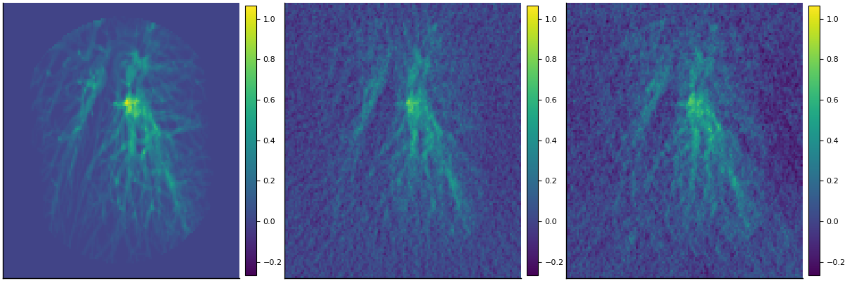
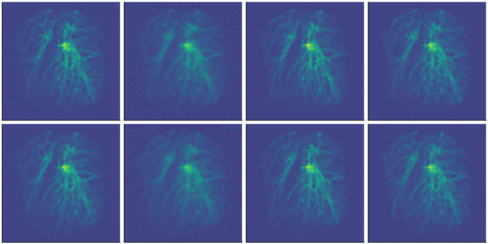
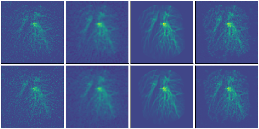
For the offline evaluation, we investigate performance on 10 blood vessel phantoms (not contained in the training set). We consider sparse sampling and Bernoulli sampling. One of the evaluation phantoms and reconstruction results for noise-free and for noisy data are shown in Figures 3-5.

To quantitatively evaluate the reconstruction quality, we calculated the relative mean absolute error (RMAE), the mean squared error (MSE), the peak signal to noise ratio (PSNR) and the structured similarity index (SSIM). The performance measures averaged over the 10 evaluation phantoms are shown in Table 1 for noise-free data, and in Table 2 for the noisy data case. We can see that the learned approaches work particular well for the sparse sampling matrix. The residual U-net seems to be better than NETT at denoising the image, which results in lower errors for noisy data. We further observe that our simple trained regularizer in any case performs better than the (very simple) deterministic one. The $\ell_{1}$-minimization approach works best for noise-free Bernoulli measurements, but it is outperformed by the learned approaches in the noisy data case. Since $\ell_{1}$-minimization needs many iterations we did not iterate until convergence; for the presented reconstructions it is already one order of magnitude slower than the other methods. In the noisy data case, we observe that the NETT yield smaller MSE than the residual U-net for Bernoulli measurements, while the U-Net approach works best for the sparse measurements.

4.4 Results for experimental data

We used experimental data measured by the PAT device using integrating line sensors as described in [34, 10]. The setup corresponds to the one used for our simulated phantoms. The first sample is a simple cross phantom and the second is a leaf phantom with many fine structures. We only test sparse measurements, since the current experimental setup does not support Bernoulli measurements. For the residual U-net and the NETT with trained regularizer we use the networks trained on the blood vessel data set as described above.

Figure 6: Reconstructions of the cross phantom from experimental data. The reconstruction results are obtained for the sparse sampling pattern using the following algorithms, from left to right: FBP, $\ell_{1}$-minimization, U-net and NETT.

Figure 7: Reconstructions of the leaf phantom from experimental data. The reconstruction results are obtained for the sparse sampling pattern using the following algorithms, from left to right: FBP, $\ell_{1}$-minimization, U-net and NETT.

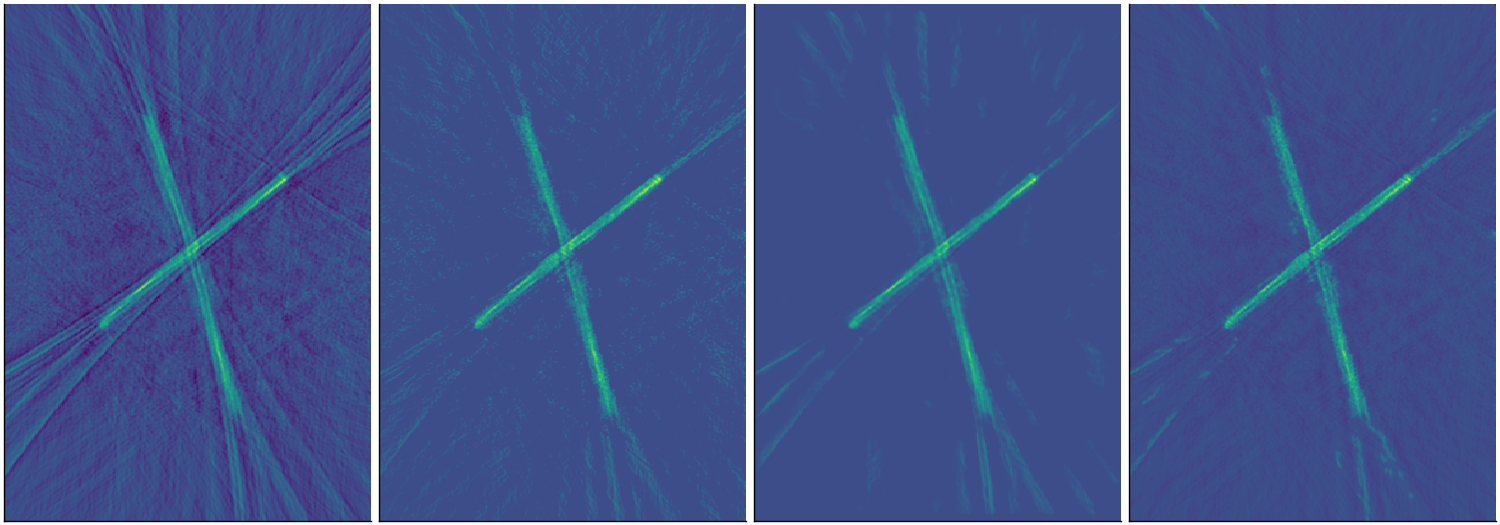
Reconstruction results for the cross phantom are shown in Figure 6. All methods yield quite accurate results and all structures are resolved clearly. However, none of the methods is able to completely remove the strong artifacts extending from the corners of the cross phantom. The U-net seems to do the best job by removing nearly all artifacts. Reconstruction results for the leaf phantom are shown in Figure 7. Reconstructing the leaf phantom is more challenging, since it contains very fine structures. None of the methods is able to resolve them completely. The artifacts outside of the object are present in all reconstructed images. However, the reconstruction using joint $\ell^{1}$-minimization and the deep-learning approaches (NETT and residual U-net) yield satisfying results. Nevertheless, future work is required to improve the reconstruction quality for real-word data.

5 Discussion and conclusion

We studied deep-learning approaches (NETT and the residual U-net) and joint $\ell_{1}$-minimization for CS-PAT using either sparse sampling or Bernoulli measurements. All methods work well for both types of measurements. For exact data, iterative approaches, which use the forward operator in each step, work better than the residual U-net for Bernoulli measurements. Incorporating different sampling strategies directly in the experimental setup is an interesting line for future research. NN based algorithms perform well with noisy data, but still are open for improvements for experimental data. This suggests that our simulated training data is different from the measured real-world data. Developing more accurate forward models and improving training data are an important future goal. The learned regularizer has a quite simple network structure. Investigating more complex network architectures and modified training strategies will be investigated in future work.

References

- [1] M. Sandbichler, F. Krahmer, T. Berer, P. Burgholzer, and M. Haltmeier, “A novel compressed sensing scheme for photoacoustic tomography,” SIAM J. Appl. Math. 75(6), pp. 2475–2494, 2015.
- [2] S. Arridge, P. Beard, M. Betcke, B. Cox, N. Huynh, F. Lucka, O. Ogunlade, and E. Zhang, “Accelerated high-resolution photoacoustic tomography via compressed sensing,” Phys. Med. Biol. 61(24), p. 8908, 2016.
- [3] M. Haltmeier, T. Berer, S. Moon, and P. Burgholzer, “Compressed sensing and sparsity in photoacoustic tomography,” J. Opt. 18(11), p. 114004, 2016.
- [4] P. Burgholzer, J. Bauer-Marschallinger, H. Grün, M. Haltmeier, and G. Paltauf, “Temporal back-projection algorithms for photoacoustic tomography with integrating line detectors,” Inverse Probl. 23(6), pp. S65–S80, 2007.
- [5] G. Paltauf, R. Nuster, M. Haltmeier, and P. Burgholzer, “Photoacoustic tomography using a Mach-Zehnder interferometer as an acoustic line detector,” Appl. Opt. 46(16), pp. 3352–3358, 2007.
- [6] M. Haltmeier, “Sampling conditions for the circular radon transform,” IEEE Trans. Image Process. 25(6), pp. 2910–2919, 2016.
- [7] S. Gratt, R. Nuster, G. Wurzinger, M. Bugl, and G. Paltauf, “64-line-sensor array: fast imaging system for photoacoustic tomography,” Proc. SPIE 8943, p. 894365, 2014.
- [8] J. Bauer-Marschallinger, K. Felbermayer, K.-D. Bouchal, I. A. Veres, H. Grün, P. Burgholzer, and T. Berer, “Photoacoustic projection imaging using a 64-channel fiber optic detector array,” in Proc. SPIE, 9323, 2015.
- [9] G. Paltauf, P. Hartmair, G. Kovachev, and R. Nuster, “Piezoelectric line detector array for photoacoustic tomography,” Photoacoustics 8, pp. 28–36, 2017.
- [10] M. Haltmeier, M. Sandbichler, T. Berer, J. Bauer-Marschallinger, P. Burgholzer, and L. Nguyen, “A sparsification and reconstruction strategy for compressed sensing photoacoustic tomography,” J. Acoust. Soc. Am. 143(6), pp. 3838–3848, 2018.
- [11] S. Antholzer, J. Schwab, and M. Haltmeier, “Deep learning versus -minimization for compressed sensing photoacoustic tomography,” in 2018 IEEE International Ultrasonics Symposium (IUS), pp. 206–212, 2018.
- [12] H. Li, J. Schwab, S. Antholzer, and M. Haltmeier, “NETT: Solving inverse problems with deep neural networks,” 2018. arXiv:1803.00092.
- [13] D. Finch, M. Haltmeier, and Rakesh, “Inversion of spherical means and the wave equation in even dimensions,” SIAM J. Appl. Math. 68(2), pp. 392–412, 2007.
- [14] H. Chen, Y. Zhang, W. Zhang, P. Liao, K. Li, J. Zhou, and G. Wang, “Low-dose CT via convolutional neural network,” Biomed. Opt. Express 8(2), pp. 679–694, 2017.
- [15] K. H. Jin, M. T. McCann, E. Froustey, and M. Unser, “Deep convolutional neural network for inverse problems in imaging,” IEEE Trans. Image Process. 26(9), pp. 4509–4522, 2017.
- [16] Y. Han, J. J. Yoo, and J. C. Ye, “Deep residual learning for compressed sensing CT reconstruction via persistent homology analysis,” 2016. http://arxiv.org/abs/1611.06391.
- [17] S. Antholzer, M. Haltmeier, and J. Schwab, “Deep learning for photoacoustic tomography from sparse data,” Inverse Probl. Sci. and Eng. in press, pp. 1–19, 2018.
- [18] S. Antholzer, M. Haltmeier, R. Nuster, and J. Schwab, “Photoacoustic image reconstruction via deep learning,” in Photons Plus Ultrasound: Imaging and Sensing 2018, 10494, p. 104944U, International Society for Optics and Photonics, 2018.
- [19] A. Hauptmann, F. Lucka, M. Betcke, N. Huynh, J. Adler, B. Cox, P. Beard, S. Ourselin, and S. Arridge, “Model based learning for accelerated, limited-view 3d photoacoustic tomography,” IEEE Trans. Med. Imaging 37(6), pp. 1382–1393, 2018.
- [20] D. Waibel, J. Gröhl, F. Isensee, T. Kirchner, K. Maier-Hein, and L. Maier-Hein, “Reconstruction of initial pressure from limited view photoacoustic images using deep learning,” in Photons Plus Ultrasound: Imaging and Sensing 2018, 10494, p. 104942S, International Society for Optics and Photonics, 2018.
- [21] O. Ronneberge, P. Fischer, and T. Brox, “U-net: Convolutional networks for biomedical image segmentation,” CoRR , 2015.
- [22] J. Schwab, S. Antholzer, and M. Haltmeier, “Deep null space learning for inverse problems: convergence analysis and rates,” Inverse Probl. 35(2), p. 025008, 2019.
- [23] J. Schwab, S. Antholzer, and H. M. Haltmeier, “Big in Japan: Regularizing networks for solving inverse problems,” 2018. arXiv:1812.00965.
- [24] S. Foucart and H. Rauhut, A mathematical introduction to compressive sensing, Applied and Numerical Harmonic Analysis, Birkhäuser/Springer, New York, 2013.
- [25] M. Grasmair, M. Haltmeier, and O. Scherzer, “Necessary and sufficient conditions for linear convergence of -regularization,” Comm. Pure Appl. Math. 64(2), pp. 161–182, 2011.
- [26] P. L. Combettes and J.-C. Pesquet, “Proximal splitting methods in signal processing,” in Fixed-point algorithms for inverse problems in science and engineering, H. H. Bauschke, R. S. Burachik, P. L. Combettes, V. Elser, D. R. Luke, and H. Wolkowicz, eds., pp. 185–212, Springer, 2011.
- [27] J. Adler and O. Öktem, “Learned primal-dual reconstruction,” IEEE Trans. Med. Imaging 37(6), pp. 1322–1332, 2018.
- [28] E. Kobler, T. Klatzer, K. Hammernik, and T. Pock, “Variational networks: connecting variational methods and deep learning,” in German Conference on Pattern Recognition, pp. 281–293, Springer, 2017.
- [29] B. Kelly, T. P. Matthews, and M. A. Anastasio, “Deep learning-guided image reconstruction from incomplete data,” arXiv:1709.00584 , 2017.
- [30] F. Chollet et al., “Keras.” https://github.com/fchollet/keras, 2015.
- [31] M. Abadi, A. Agarwal, P. Barham, et al., “TensorFlow: Large-scale machine learning on heterogeneous systems,” 2015. Software available from tensorflow.org.
- [32] J. Schwab, S. Antholzer, R. Nuster, and M. Haltmeier, “Real-time photoacoustic projection imaging using deep learning,” 2018. arXiv:1801.06693.
- [33] D. P. Kingma and J. Ba, “Adam: A method for stochastic optimization,” 2014. arXiv:1412.6980.
- [34] J. Bauer-Marschallinger, K. Felbermayer, and T. Berer, “All-optical photoacoustic projection imaging,” Biomed. Opt. Express 8(9), pp. 3938–3951, 2017.