Sliced Inverse Regression: application to fundamental stellar parameters

Abstract

We present a method for deriving stellar fundamental parameters. It is based on a regularized sliced inverse regression (RSIR). We first tested it on noisy synthetic spectra of A, F, G, and K-type stars, and inverted simultaneously their atmospheric fundamental parameters: $T_{\mathrm{eff}}$, $\log g$, $[M/H]$  and $v\sin i$. Different learning databases were calculated using a range of sampling in $T_{\mathrm{eff}}$, $\log g$, $v\sin i$, and $[M/H]$. Combined with a principal component analysis (PCA) nearest neighbors (NN) search, the size of the learning database is reduced. A Tikhonov regularization is applied, given the ill-conditioning of SIR. For all spectral types, decreasing the size of the learning database allowed us to reach internal accuracies better than PCA-based NN-search using larger learning databases. For each analyzed parameter, we have reached internal errors that are smaller than the sampling step of the parameter. We have also applied the technique to a sample of observed FGK and A stars. For a selection of well studied stars, the inverted parameters are in agreement with the ones derived in previous studies. The RSIR inversion technique, complemented with PCA pre-processing proves to be efficient in estimating stellar parameters of A, F, G, and K stars.

1 Introduction

Astronomical surveys, either spaceborne or ground-based, are gathering an unprecedented amount of data. One can mention the SDSS DR14 data (Abolfathi et al., 2018) that contains 154 TB of millions of spectroscopic and photometric data. The DR5 of the LAMOST survey (Cui et al., 2012) contains 9 million spectra in total. Gaia DR2 provides information about 1.3 billion stars (Katz & Brown, 2017). These space and ground-based surveys quantify the size of the data the astronomical community will face in a near future.

Spectroscopic analysis is crucial for the derivation of fundamental stellar atmospheric parameters which are the effective temperature ($T_{\mathrm{eff}}$), the surface gravity ($\log g$), and the metallicity ($[M/H]$). In addition to these fundamentals, and because it may strongly affect the shape of the observed spectra, the projected equatorial rotational velocity, $v\sin i$, is also retrieved from spectroscopic information. Many authors have for long been using spectroscopic data to estimate the stellar atmospheric parameters (McWilliam, 1990, Latham et al., 2002, Torres et al., 2002, Buchhave et al., 2012, Schönrich & Bergemann, 2014, Dieterich et al., 2017, Fabbro et al., 2018). However in order to extract the most relevant and accurate information from high-resolution, and large bandwidths stellar spectra, still more endeavour is required.

Most of the traditional approaches and developed pipelines rely on standard procedures such as comparing an observed spectrum with a set of theoretical spectra (Valenti & Piskunov, 1996, Morris et al., 2018). The requirement for advanced computational techniques rises from the generated large dimensionality of the data due to the wide wavelength coverage together with high spectral resolution. Many new techniques are being developed. In Ness et al. (2015) and Casey et al. (2016), a data-driven approach is introduced (CANNON) for determining stellar labels (fundamental parameters and detailed stellar abundances) from spectroscopic data. Their learning databases (LDB) are based on a subset of reference objects for which the stellar labels are known with high accuracy. Dimension reduction techniques are also developed and used, such as applying the Principal Component Analysis (PCA) for data reduction (see e.g. Jolliffe 1986). PCA has shown its effectiveness in inverting the fundamental stellar atmospheric parameters in several studies (Bailer-Jones et al., 1998, Re Fiorentin et al., 2007, Paletou et al., 2015a, b, Gebran et al., 2016). Xiang et al. (2017) estimated the stellar atmospheric parameters as well as the absolute magnitudes and $\alpha$-elements abundances from the LAMOST spectra with a multivariate regression method based on kernel-based PCA. The LAMOST spectroscopic survey data has also been recently analyzed by Boeche et al. (2018) to invert stellar parameters and chemical abundances in which several combined approaches and techniques were compared. The authors developed a code called SP_Ace which utilizes nearest neighbor comparison and non-linear model fitting techniques. In Wilkinson et al. (2017), a spectral fitting code (FIREFLY) was developed to derive the stellar population properties of stellar systems. FIREFLY uses a $\chi$-squared minimization fitting procedure that fits stellar population models to spectroscopic data, following an iterative best-fitting process controlled by a Bayesian information criterion. Their approach is efficient to overcome the so-called ``ambiguities'' in the spectra. More recently, Gill et al. (2018) used wavelet decomposition to distinguish between noise, continuum trends, and stellar spectral features in the CORALIE FGK-type spectra. By calculating a subset of wavelet coefficients from the target spectrum and comparing it to those from a grid of models in a Bayesian framework, they were able to derive $T_{\mathrm{eff}}$, $[M/H]$, and $v\sin i$ for these stars. Ting et al. (2018) presented The Payne, a general method for the precise and simultaneous determination of numerous stellar labels from observed spectra. Using a simple neural-net-like functional form and a suitable choice of training labels, The Payne yields a spectral flux prediction good to $10^{-3}$ rms across a wide range of $T_{\rm eff}$ and $\log g$. Ting et al. (2018) applied this approach to the APOGEE DR14 data set and obtained precise elemental abundances of 15 chemical species. In the same context, Fabbro et al. (2018) applied a deep neural network architecture to analyse both SDSS-III APOGEE DR13 and synthetic stellar spectra. Their convolutional neural network model, StarNet, was able to predict precise stellar parameters when trained on APOGEE spectra or on synthetic data.

In this study, we apply techniques such as, reduction of dimensionality with PCA, and a PCA-based nearest neigbor search (Paletou et al., 2015a, b, Gebran et al., 2016) complemented with a Regularized Sliced Inverse Regression (Bernard-Michel et al., 2009, 2007) (RSIR) procedure in order to derive simultaneously $T_{\mathrm{eff}}$, $\log g$, $[M/H]$  and $v\sin i$ from spectra of A, and FGK type stars. Up to now, sliced inverse regression has been rarely used in astronomy (Bernard-Michel et al., 2009, Watson et al., 2017). When combined with PCA-based techniques, the derivations of the fundamental atmospheric parameters are achieved with higher accuracy compared to the sole/mere PCA-based nearest neighbor inversion (Paletou et al., 2015a, b, Gebran et al., 2016). The mathematical description of our method is detailed in Sec. 2. Section 3 describes all elements used for the enhancement of the computational abilities of SIR. Section  4 discusses the application of the technique on synthetic spectra for A, F, G, and K-type like stars. In section  5, we show the results of inversions of real stars. Discussion and conclusion are gathered in Sec. 6.

2 Sliced inverse regression (SIR)

SIR, originally formulated by Li (1991), is a statistical technique that reduces multivariate regression to a lower dimension. It finds an inverse functional relationship between the response and the predictor which are the fundamental parameters and the flux respectively. Synthetic spectra flux values, $x_{syn}$, are usually calculated based on the set of stellar atmospheric parameters in the form of:

$$x_{syn}=f(T_{\mathrm{eff}}\ ,\log g\ ,[M/H]\ ,v\sin i)\,.$$ (1)

The inverse functional relation is used to predict the parameters of the observed flux values, $x_{obs}$, in the form of:

$$f^{-1}(x_{obs})=(T_{\mathrm{eff}}\ ,\log g\ ,[M/H]\ ,v\sin i)\,.$$ (2)

In our work, we have derived a functional relationship for each parameter in the following way:

$$Y_{j}=f^{-1}_{j}(x_{obs})\,,$$ (3)

where $j=1,2,3,4$ for $T_{\mathrm{eff}}$, $\log g$, $[M/H]$, and $v\sin i$.

2.1 Global covariance matrix $\Sigma$

SIR starts with the computation of the covariance matrix $\Sigma$ of all the synthetic spectra $x_{i}$ of the LDB:

First, spectra are gathered in a matrix of dimension $N_{spectra}$ $\times$ $N_{\lambda}$, where $N_{\lambda}$ is the number of wavelength points per spectrum and $N_{\mathrm{spectra}}$ is the total number of spectra in the LDB. Then, the covariance matrix $\Sigma$, is defined as:

$$\Sigma=\frac{1}{N_{\mathrm{spectra}}}\sum_{i=1}^{N_{\mathrm{spectra}}}(x_{i}-\overline{x}).(x_{i}-\overline{x})^{T}\,,$$ (4)

where the global mean $\overline{x}$ is defined as:

$$\overline{x}=\frac{1}{N_{\mathrm{spectra}}}\sum_{i=1}^{N_{\mathrm{spectra}}}x_{i}\,,$$ (5)

$x_{i}$ being a row vector containing the flux values of spectrum $i$.

2.2 Intra-slices covariance matrix

In SIR, all spectra are organized based on an increasing order of the considered parameter for inversion. For example, if we are to invert $T_{\mathrm{eff}}$  of each star, the spectra database should be organized in increasing order of $T_{\mathrm{eff}}$ while having the other parameters ordered randomly. We then build-up subsets of spectra, also called ``slices'', having the same value of the parameter one wishes to determine first. These slices should not overlap each other (Li, 1991). Then we calculate the means $\overline{x}_{h}$ of the slice of the spectra found in each slice $S_{h}$ that contains $n_{h}$ synthetic spectra (h being the index of each slice). For the inversion of each parameter, $\overline{x}_{h}$ and $\overline{x}$ are used to calculate the ``intra-slices'' covariance matrix, $\Gamma$:

$$\Gamma=\sum_{h=1}^{H}\frac{n_{h}}{N}(\overline{x}_{h}-\overline{x}).(\overline{x}_{h}-\overline{x})^{T}\,,$$ (6)

where

$$\overline{x}_{h}=\frac{1}{n_{h}}\sum_{x\epsilon S_{h}}x_{i}\,.$$ (7)

2.3 Dimension reduction and parameter inversion

SIR aims to build a reducing subspace that maximizes the variance between the slices while minimizing the variance within the slices which creates a reduced predictor versus response regressive relationship to predict the parameters of the observed stars. This is applied by the process of stacking the spectra by an increase order of similar or close valued parameters and averaging them into a single spectra and projecting them on a new subspace. These new projection will later be used predictors of the functional relationship. Since the reduced projections are formed from spectra having close parameter values, this insures a higher accuracy of regressive predictions (Watson et al., 2017). On the other hand, slicing the spectra based on non-overlapping similar parameters insures this inter-slice maximization and intra-slice minimization.

The matrix $\Sigma^{-1}\Gamma$ is then calculated where $\Sigma$ and $\Gamma$ are the two previously defined matrices. One eigenvector of $\Sigma^{-1}\Gamma$, called $\beta_{\lambda}$ and corresponding to an eigenvalue $\lambda$, is used to form the reduction subspace. This will allow us to do regression in a 2-dimensional space using an inverse functional relationship. This relationship is constructed via a linear piecewise interpolation between the projection coordinates of the slices on the single eigenvector of $\Sigma^{-1}\Gamma$ and the parameters.

The selection of $\beta_{\lambda}$, is based on a metric $C_{\lambda}$ that quantifies the relationship between the spectra and the parameters. $C_{\lambda}$, defined as the ``sliced inverse regression criteria'' (Bernard-Michel et al., 2007, 2009), is calculated as follows:

$$C_{\lambda}=\frac{\beta_{\lambda}^{t}\,\Gamma\,\beta_{\lambda}}{\beta_{\lambda}^{t}\,\Sigma\,\beta_{\lambda}}\approx\frac{Var(<\beta_{\lambda}\,.\,x_{i}>)}{Var(<\beta_{\lambda}\,.\,x_{i}>)+Var(S_{h})}\,,$$ (8)

where $\beta_{\lambda}^{t}$ is the transpose of $\beta_{\lambda}$ and $Var$ is the variance function

$\beta_{\lambda}^{t}\,\Gamma\,\beta_{\lambda}$ is the ``inter-slice'' variance, whereas $\beta_{\lambda}^{t}\,\Sigma\,\beta_{\lambda}$ represents the total variance. The $\beta_{\lambda}$ that gives a $C_{\lambda}$ value closest to 1 is considered as a the best choice for the reducing basis vector. In the present work, $C_{\lambda}$ varies between 0.91 and 0.97 when using the eigenvector of $\Sigma^{-1}\Gamma$ with the largest eigenvalue $\lambda$.

To invert the parameters, we apply linear piecewise interpolation on the coordinates of the projections of the $\overline{x}_{h}$-s on $\beta_{\lambda}$. Finally, the estimation of the parameters is made according to:

$$\widehat{y}=\begin{cases}\overline{y}_{1},&\mbox{if }x^{p}\mbox{ $\epsilon]-\infty,\overline{x}_{1}^{p}]$ },\\ \overline{y}_{h}+\bigg{(}x_{obs}^{p}-\overline{x}_{h}^{p}\bigg{)}\bigg{(}\frac{\overline{y}_{h+1}-\overline{y}_{h}}{\overline{x}_{h+1}^{p}-\overline{x}_{h}^{p}}\bigg{)}&\mbox{if }x^{p}\mbox{ $\epsilon]\overline{x}_{h}^{p},\overline{x}_{h+1}^{p}]$ },\\ \overline{y}_{H},&\mbox{if }x^{p}\mbox{$\epsilon]\overline{x}^{p}_{H},+\infty$[ },\end{cases}$$ (9)

where $\widehat{y}$ is the estimated parameter; $\overline{y}_{h}$ is the mean of the parameters of the spectra in slice $h$. The superscript ``p'' represents the projected value of a selected set of data on $\beta_{\lambda}$ i.e., $x^{p}=<\beta_{\lambda}\,.\,x>$.

3 Enhancement of the computational abilities of SIR

In the present work, we are dealing with large amounts of high resolution spectra, so that $\Sigma^{-1}\Gamma$ have typical dimension of $\sim 10^{4}\times 10^{4}$. In addition, using a large LDB for SIR induces an increase in the intra-slice variance. This will lead to less accurate inverted parameters. Therefore to simultaneously address these problems, we applied two additional steps to SIR: first, using PCA, we reduce the dimension of every spectra in the LDB (Watson et al., 2017) from $\sim 10^{4}$ to $12$. Second, we apply a PCA-based NN-search in the reduced subspace to select a smaller LDB, more relevant for the spectra one wishes to analyze.

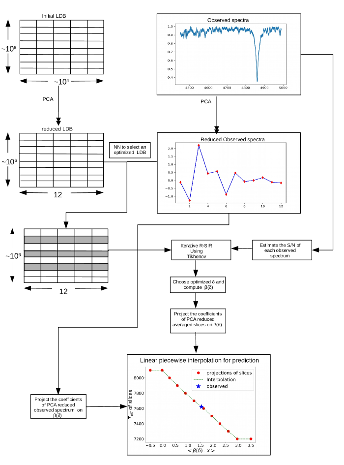
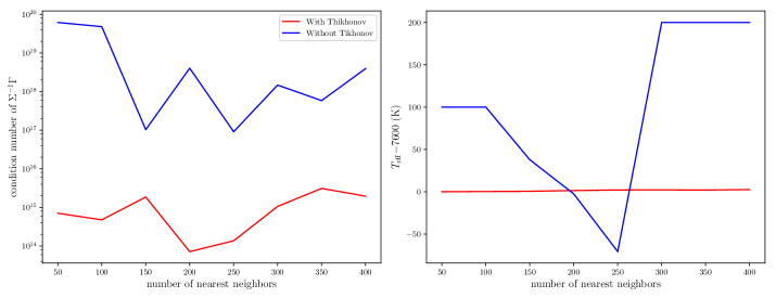
$\Sigma^{-1}\Gamma$ matrix is generally ill-conditioned. And the higher the condition number is, the more noise sensitive the system becomes (Kreyszig, 2010). For the present work, values as large as $10^{20}$ were found. In that case $\beta_{\lambda}$ is very noise sensitive, leading to an unstable functional relationship. As a result, inaccurate inverted parameters may be derived. To solve this issue, we have applied Tikhonov regularization which aims to improve the conditioning of $\Sigma^{-1}\Gamma$ and add a priori information to it based on the analysis of the noise of each observed spectrum. Several regularization methods exist, however, Tikhonov is very common and easily implemented. Other studies may address this issue, such as the truncated SVD used in Watson et al. (2017). Figure 1 summarizes the successive procedures we implemented, and that we discuss with more details hereafter.

3.1 LDB reduction via PCA

PCA is a numerical technique that allows for the reduction of dimension of each spectrum by projecting it on a set of orthogonal basis vectors called principal components (PC's). These components are the eigenvectors of the global covariance matrix $\Sigma$. Paletou et al. (2015a) and Gebran et al. (2016) showed that for databases similar to the ones used in this study, only 12 PC's associated to the largest eigenvalues are enough to reduce the LDB, while the reconstruction error remains less than 1%. Therefore after this first pass, the new LDB has dimension of $N_{spectra}\times 12$.

The original LDB may reach to a dimension of $N_{spectra}\times N_{\lambda}\simeq$ $10^{6}\times 10^{4}$. This is due to the fine sampling in the parameters, the high dimension of the spectra, and the large wavelength range which makes the process of SIR computationally heavy in terms of memory and time. To reduce the LDB which will be used for SIR, for each observed star, a PCA-based nearest neighbor search in the reduced subspace is applied (Paletou et al., 2015a). This is done using the ``PCA distance'' $d_{j}^{(O)}$, defined as:

$$d^{(O)}_{j}=\sqrt{\Sigma^{12}_{k=1}(\varrho_{k}-p_{jk})^{2}}\,,$$ (10)

where $\varrho_{k}$ is the projection coordinate on the $k^{th}$ dimension for an observed spectrum, and $p_{jk}$ is the projection coefficient on the $k^{th}$ dimension for the $j^{th}$ synthetic spectrum. Finally for the SIR, a set of NN will be selected for each observed star as we will later describe in sec. 3.3.

3.2 Tikhonov regularization

Fig. 1: Flowchart of the procedure. The numerics in this figure are for the inversions of the test described in Sec. 3.

For the Tikhonov method (Vogel, 2002), one usually inserts a regularization parameter $\delta>0$ into the ill-conditioned system, usually based on a priori information gathered by analyzing the noise of each observed spectrum. Considering the following matrix:

$$(\Sigma^{2}+\delta I)^{-1}\Sigma\Gamma\,.$$ (11)

The eigenvector $\beta_{\lambda}(\delta)$ associated to the largest eigenvalue of the matrix defined in Eq. 11 is calculated based on an optimization approach. For each parameter of each observed star, an optimum and specific $\delta$ is calculated. This procedure is initiated by estimating the signal to noise ratio (S/N) of the observed spectrum using the procedure of Stoehr et al. (2008). Then a random set of synthetic spectra are selected from the LDB, and Gaussian white noise having the same S/N as the one of the observed spectrum is added to them. SIR is finally applied to this selected random set and the prediction of their parameters is done via the piecewise interpolation process described in Eq. 9. This simulated inversion leads to the selection of an optimum $\beta_{\lambda}(\delta)$.

$\delta$ is estimated by minimizing the difference between the newly inverted parameter values of the randomly selected noise added spectra ($\widehat{y}_{i}$) and their initial noiseless values ($y_{i}$). The comparison is done using a normalized $\chi^{2}$:

$$\chi^{2}_{N}=\sqrt{\frac{\sum_{i=1}^{n}(\,\widehat{y}_{i}-y_{i})^{2}}{\sum_{i=1}^{n}(\,y_{i}-\overline{y}_{i})^{2}}}\,.$$ (12)

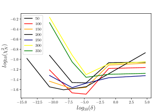
It was found that $log_{10}(\chi^{2}_{N})$ as a function of $log(\delta)$ is a unimodal function which has a local minimum. This function is displayed in Fig. 3 for a synthetic spectrum having $T_{\mathrm{eff}}$, $\log g$, $[M/H]$ , $v\sin i$  and S/N of 7 600 K, 2.50 dex, 0.0 dex, and 197 $\mbox{km}\,\mbox{s}^{-1}$, and 196, respectively. The original LDB used in this example is the one of Gebran et al. (2016), explained in detail in Sec. 4. To find the minimum of these curves, we applied a golden-section search algorithm (Kiefer, 1953). It is a classical numerical technique that minimizes unimodal functions which have a global minimum. The inversion process for each analyzed spectrum, and each parameter, has its own $\chi^{2}_{N}=f(\delta)$ that needs to be minimized.

3.3 Integrated scheme of the enhancements

Now that we have described the tools that were used to improve the SIR procedure, in what follows we discuss how these techniques are integrated to increase the accuracy of the inversion process. The flowchart in Fig. 1 summarizes our adopted approach.

In our work $\Sigma$ and $\Sigma^{-1}\Gamma$ have reached dimensions of the order of $\sim 10^{4}\times 10^{4}$. For that reason and before applying the SIR process for each spectrum to be analyzed, we have reduced the dimension of these matrices by reducing the size of the original LDB using PCA as described in sec. 3.1.

During SIR, at least two distinct parameter values for each slice are required to construct the functional relationship. Therefore to select the optimum reduced LDB, a test for the construction of this relationship is required. Iteratively we tested for the number of distinct parameters by increasing the number of spectra of the nearest nearest neighbors. Whenever the values of the distinct concerned parameters become greater or equal to 2, the iteration breaks and the inversion proceeds to the interpolation. During the tests, there were situations where $[\Sigma^{2}+\delta I]^{-1}$ was singular. This iterative approach solved this problem by adding nearest neighbors. Generally, using a smaller LDB which contain only a set of closest spectra to the observed one theoretically insures the success of SIR compared to using the entire original LDB. When selecting a set of nearest neighbors, we insure a lower minimization value of the intra-slice variance $Var(S_{h})$ in Eq. 8. Now within each slice the spectra are closer to each other and they are closer to the average spectrum of the slice. At the same time, choosing these optima reduced LDB's overcomes the issue of the degeneracies. In the PCA based NN-search (Paletou et al., 2015a, Gebran et al., 2016), we had cases where the $d_{j}^{(O)}$ where extremely close to each or even equal, with a variety of parameters. In SIR, we do not face such issue because the value are regressed for each parameter and the synthetic spectra with similar or close parameters are averaged to a single slice.

Now $\Sigma^{-1}\Gamma$ has a dimension of $12\times 12$ and is constructed from the optimized reduced LDB. Its high condition number implies that it is ill-conditioned (see the example of the left panel of Fig .2). Therefore to improve the inversion process for each observed spectrum, we apply the Tikhonov regularization in SIR for our selected optima reduced LDB's, iteratively. By applying this regularization, we are effectively taking advantage of the S/N ratio analysis and inserting the propagated noise information as a priori. In other words, we are applying an denoising procedure.

In Fig. 2, we display the inversion results for $T_{\mathrm{eff}}$ of a noisy synthetic spectrum. This spectrum has a $T_{\mathrm{eff}}$ value of 7600 K with an added Gaussian white noise of S/N = 196. As we iterate over different sizes of optimized reduced LDB's, a convergence is achieved in every case. For all of our tests, we noticed that the number of spectra in the optimized reduced LDB's did not surpass 500. It is shown in this figure that the condition number of the non-regularized matrix is $\sim$ 5 orders of magnitude larger than the ones in which the Tikhonov regularization was applied. The right panel displays the effect of the regularization on the inverted parameter ( $T_{\mathrm{eff}}$ ) of the same spectrum. It is clearly shown that whatever the number of the nearest neighbors in the optimized reduced LDB is, inversion is achieved with higher accuracy than the one without regularization. The convergence occurs irrespectively of the value of the condition number, as long as it is smaller than the one without Tikhonov regularization.

Figure 3 represents the minimization of the $log_{10}(\chi_{N}^{2})$ as a function of $log_{10}(\delta)$ for different sets of optimized reduced LDB's. This figure shows the unimodal nature of the curves irrespective of the size of the LDB.

4 Simulations and tests

In this section, we present the implementation and results of RSIR for two different sets of synthetic spectra. We also compare these results to the ones of the PCA NN-search to show the improvement in the accuracies of the derived parameters. To each of these spectra, white Gaussian noise was added with a random S/N. The spectra were calculated in the range of A to K type stars. The reason for selecting this spectral range is that in Sec. 5, we apply this procedure to a sample of the observed stars studied in Paletou et al. (2015a) and Gebran et al. (2016).

Fig. 2: Left: variation of the condition number as a function of the number of nearest neighbor using the optimum reduced LDB with and without the Tikhonov regularization. Right: the inverted $T_{\mathrm{eff}}$ as a function of the number of nearest neighbor with and without Tikhonov regularization. The inversion is done for a noise added synthetic spectrum with $T_{\mathrm{eff}}$=7600 K, $\log g$=2.50 dex, $[M/H]$=0 dex, $v\sin i$=197 $\mbox{km}\,\mbox{s}^{-1}$ and S/N= 196. For clarity we display on the value of $T_{\mathrm{eff}}$-7600 K

Fig. 3: $log_{10}(\chi^{2}_{N})$ versus $log(\delta)$ for $T_{\mathrm{eff}}$  of a synthetic spectra having $T_{\mathrm{eff}}$=7 600 K, $\log g$=2.50 dex, $v\sin i$=197 $\mbox{km}\,\mbox{s}^{-1}$, and with a S/N of 196. Each curve displays the minimization using different sets of nearest neigbor generated iteratively.

4.1 The learning databases

As done in Paletou et al. (2015b) and Gebran et al. (2016), model atmospheres were calculated using ATLAS9 with the new opacity distribution function (Kurucz, 1992, Castelli & Kurucz, 2003). These models assume local thermodynamic equilibrium (LTE), hydrostatic equilibrium, and a 1D plane–parallel atmosphere. Convection was treated using a mixing length parameter of 0.5 for 7 000 K $\leq T_{\mathrm{eff}}\leq$ 8 500 K, and 1.25 for $T_{\mathrm{eff}}\leq 7\,000$K, following the prescriptions of Smalley (2004). Synthetic spectra were calculated using SYNSPEC48 (Hubeny & Lanz, 1992). The adopted line lists were from Kurucz gfhyperall.dat and modified with more recent and accurate atomic data retrieved from the VALD and the NIST databases (for more details see Gebran et al. 2016). The calculation time for one spectrum depends mainly of the selected wavelength range. For instance, calculating one spectrum in the range of 4450-4990 Å at a resolution of 76 000 requires $\sim$20 seconds on a personal computer. Around 500 days were necessary for the calculation of the A stars LDB used in Sec. 4.2. For the wavelength range between 5000-5400 Å, one spectrum requires $\sim$22 seconds.

Table 1: Ranges of the parameters used for the calculation of the A and FGK synthetic spectra LDB's

Parms	A stars	F/G/K
$T_{\mathrm{eff}}$ (K)	[6 800,11 000]	[4 000,8 000]
$\log g$ (dex)	$[2.0,5.0]$	$[3.0,5.0]$
$[M/H]$(dex)	$[-2.0,2.0]$	$[-1.0,1.0]$
$v\sin i$ ($\mbox{km}\,\mbox{s}^{-1}$)	$[0,300]$	[0,100]
$\lambda/\Delta\lambda$	76 000	50 000

4.2 Inversion of simulated A stars

We used the LDB of Gebran et al. (2016) in which the effective temperature of the data varies from 6 800 up to 11 000 K. The wavelength region was chosen between 4 450$-$4 990 Å. This wavelength region harbors lines that are sensitive to all stellar parameters, and insensitive to microturbulent velocity which was adopted to be $\xi_{t}$=2 km/s based on the work of Gebran et al. (2016, 2014). The adopted resolution is 76 000 as it corresponds to most of the analyzed stars in Sec. 5. The ranges of all parameters in the A-star LDB are summarized in Tab. 1.

Table 2: Result of inversion for A stars using 3 different LDB's with different steps on 1 500 noisy synthetic spectra

Test	Parms	step	$\Lambda_{RSIR}$	$\Lambda_{PCA}$	offsetRSIR	offsetPCA
1	$T_{\mathrm{eff}}$ (K)	100	100.3	132	63.45	61.128
	$\log g$ (dex)	0.1	0.12	0.133	0.042	0.047
	$[M/H]$ (dex)	0.1	0.058	0.066	-0.0102	-0.0057
	$v\sin i$ (Km/s)	2: [0-20]	5.92	6.47	-0.279	0.144
		5: [20-40]
		10: [40:300]
2	$T_{\mathrm{eff}}$ (K)	200	108	190	67.54	69.33
	$\log g$ (dex)	0.2	0.109	0.145	0.03	0.04
	$[M/H]$ (dex)	0.2	0.072	0.107	-0.0102	-0.01
	$v\sin i$ (Km/s)	10	9.63	10.25	-3.5	-1.82
3	$T_{\mathrm{eff}}$ (K)	400	174	295	40.74	92.39
	$\log g$ (dex)	0.4	0.17	0.224	0.014	0.061
	$[M/H]$ (dex)	0.3	0.081	0.113	-0.016	0.0015
	$v\sin i$ (Km/s)	20	12.05	11.23	-4.11	-0.9

Noise added synthetic spectra were calculated to be used as simulated observations. Around 1 500 spectra were calculated for A stars with parameters randomly selected within the range of the LDB but not necessarily at the grid points. To analyze the effect of the sampling on the RSIR technique, we have inverted these spectra using 3 different LDB's. For the same range in all the parameter only the step was modified in each database. As an example, in the LDB 1, $T_{\mathrm{eff}}$ has a step of 100 K, whereas in LDB's 2 and 3, the steps are 200 K and 400 K, respectively. The same was done for all parameters and the details about the steps are found in Tab. 2. The sampling of the $v\sin i$ in the LDB's is not constant and depends on the value of $v\sin i$ (Gebran et al., 2016).

To compare the results of the inversion of PCA NN-search and RSIR for 1 500 spectra, we estimate the root mean square error for both techniques, $\Lambda$, defined as:

$$\Lambda=\sqrt{\frac{\sum_{i=0}^{N}(\,y_{i}^{\rm{(inv)}}-y_{i}^{\rm{(true)}}\,)^{2}}{N}}\,,$$ (13)

where $y_{i}^{\rm{(true)}}$ is the known parameter of the $i^{th}$ synthetic spectrum and $y_{i}^{\rm{(inv)}}$ its corresponding inverted one.

Columns 4 and 5 of Tab. 2 display the $\Lambda$ results using the PCA NN-search and the RSIR for the 3 LDB's. The offsets, calculated as a signed mean difference, between the inverted and the true values are presented in the last two columns of Tab. 2. Comparing the $\Lambda$ values of each approach, an improvement is achieved using RSIR for all parameters. One exception exists in the case of $v\sin i$  for test 3. The large $v\sin i$ step of the original LDB causes the PCA NN-search pre-processing stage to select inaccurate NN's. For most cases RSIR with a coarse sampling in parameters is producing more accurate inversions compared to PCA with a denser sampling. This directly infers a gain in computational time as a coarse sampling leads to smaller LDB. The time required to invert the parameters of one synthetic spectrum depends on the computational facilities. For instance, the gain in time for using the A-stars LDB of test 2 instead of the one of test 1 is $\sim$25%.

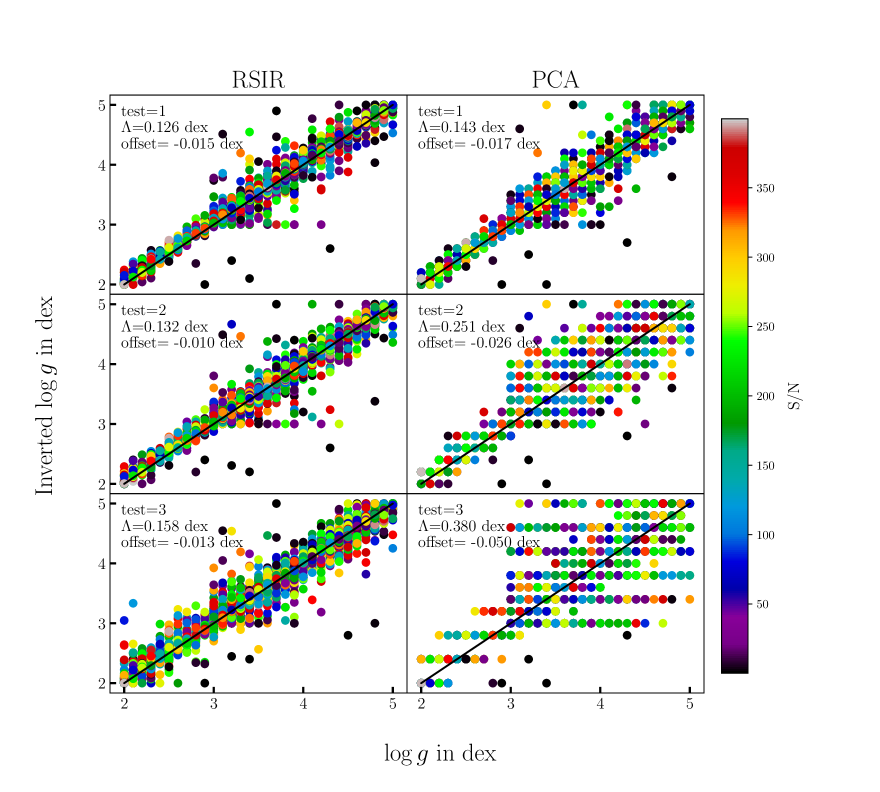
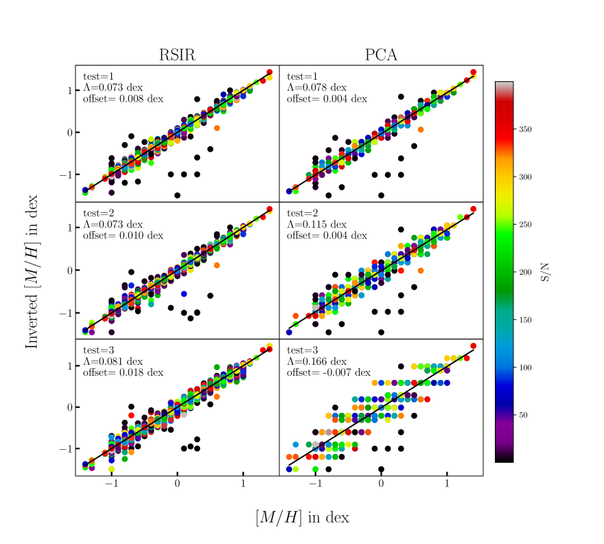
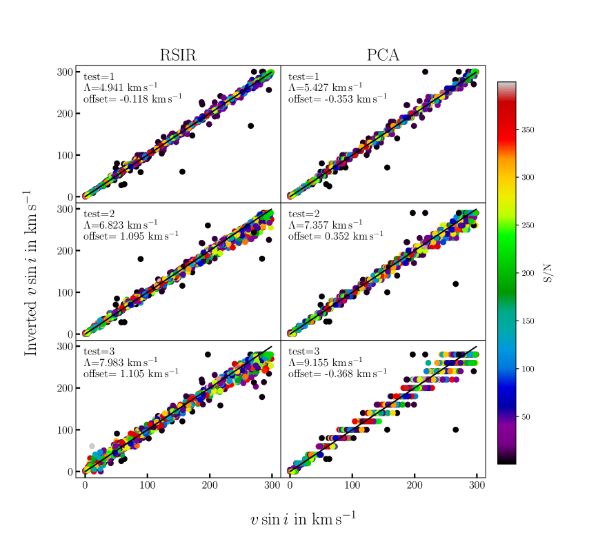
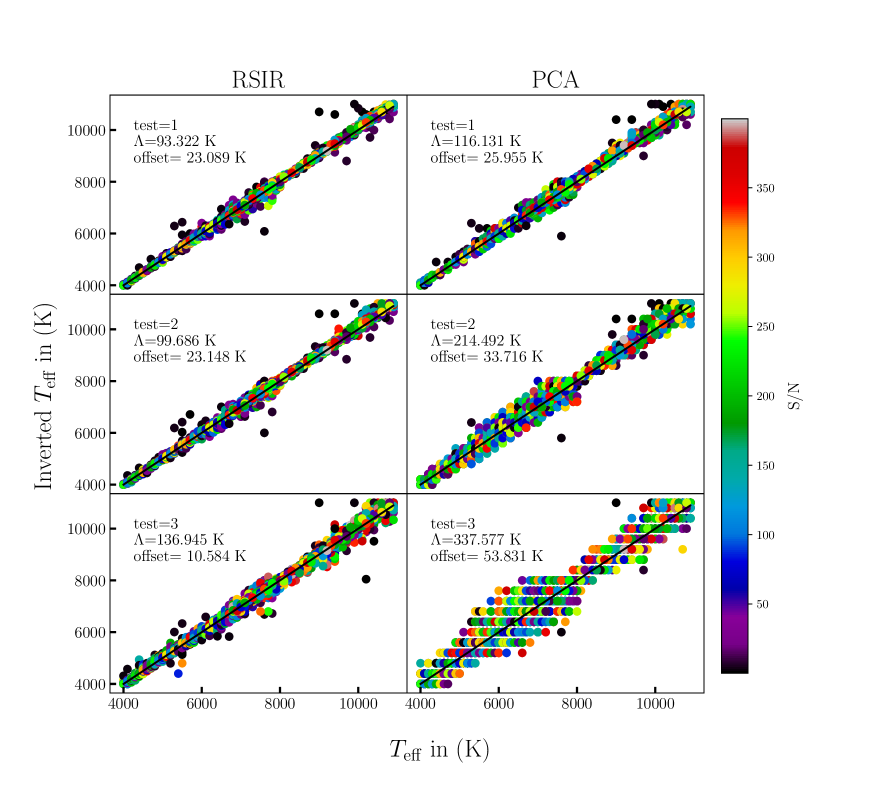
To analyze the effect of the S/N on the inversions, we display in Fig. 4 the inverted $T_{\mathrm{eff}}$ as a function of the real $T_{\mathrm{eff}}$ for the 1500 A star spectra, for different S/N and different LDB's (tests 1, 2 and 3). The results of the PCA NN-search is affected both by the sampling size and the S/N of the analyzed stars, whereas for RSIR, with the pre-processing of PCA and a Tikhonov regularization this effects becomes less significant on the accuracy of the inversion. In the appendix, we present the behavior of the inversion of $\log g$, $[M/H]$, and $v\sin i$. A similar behavior to the one of $T_{\mathrm{eff}}$ can be concluded for these parameters and this can be shown in Figs. 8, 9 and 10.

Fig. 4: Results of the effective temperature inversion for the synthetic A to K stars. The black line represents the 1-to-1 correspondance.

4.3 Inversion of Simulated FGK type stars

The same procedure was applied to FGK star-like spectra. Around 2 500 noisy spectra were produced in the ranges described Tab. 1. As done for the A stars, the parameters of the FGK synthetic spectra were also selected randomly. The chosen resolution of 50 000 is the same used in Paletou et al. (2015a). The wavelength range was selected from 5 000 to 5 400 Å  containing the Mg i b triplet, a good indicator of $\log g$ and sensitive as well to $T_{\mathrm{eff}}$. The microturbulent velocity was set to $\xi_{t}$ $\sim$ 1 $\mbox{km}\,\mbox{s}^{-1}$(Gebran et al., 2014). The inversion results ($\Lambda$ and offsets) as a function of the sampling steps are shown in Tab. 3. These results show similar behavior to that of the A stars in terms of improvement in accuracy while comparing RSIR to PCA NN-search. In Fig. 4 we also overplot the $T_{\mathrm{eff}}$ for our F/G/K noisy synthetic spectra. The effect of inversion as a function of S/N and sampling is very similar to the one of A stars, and for all the parameters (Figs. 8, 9 and 10).

Table 3: Result of inversion using 3 different LDB's with different steps on 2 500 noisy synthetic FGK spectra

Test	parms	step	$\Lambda_{RSIR}$	$\Lambda_{PCA}$	offsetRSIR	offsetPCA
1	$T_{\mathrm{eff}}$ (K)	100	106	117	5.92	0.04
	$\log g$ (dex)	0.1	0.121	0.136	0.016	0.002
	$[M/H]$ (dex)	0.1	0.061	0.063	-0.45	-0.56
	$v\sin i$ (Km/s)	2: [0-20]	1.72	2.88	0.005	0.06
		5: [20-40]
		10: [40-100]
2	$T_{\mathrm{eff}}$ (K)	200	109	236	8.17	-7.86
	$\log g$ (dex)	0.2	0.132	0.289	0.0027	-0.017
	$[M/H]$ (dex)	0.2	0.066	0.115	-0.47	-0.62
	$v\sin i$ (Km/s)	2: [0-20]	1.88	3.17	0.0087	0.0004
			10: [20-40]
			10: [40-100]
3	$T_{\mathrm{eff}}$ (K)	400	127	368	10.43	-27
	$\log g$ (dex)	0.4	0.147	0.45	-0.01	-0.04
	$[M/H]$ (dex)	0.4	0.07	0.17	-0.84	-0.625
	$v\sin i$ (Km/s)	4: [0-20]	2.25	5.243	0.018	-0.011
		10: [20-40]
		10: [40-100]

5 Application to observed spectra

Fig. 5: Comparison between the inverted parameters for our FGK stars sample (filled circles) and A stars (filled triangle).

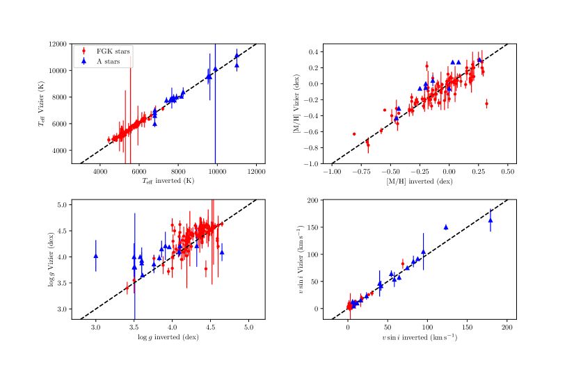
The performance of the RSIR has been tested on two samples of stellar spectra. The first sample is the one of the Spectroscopic Survey of Stars in the Solar Neighborhood (S⁴N, Allende Prieto et al. 2004). These are spectra of bright FGK stars that are at distance less than 15 pc. We have estimated the S/N of these spectra in the wavelength range used for the inversion of the parameters [5 000$-$5 400Å]. This ratio ranges between 40 and 450. These spectra are at a resolution of $\lambda/\Delta\lambda\sim$50 000. All the details about the acquisition and the reduction procedure of the S⁴N data can be found in Allende Prieto et al. (2004). These spectra were inverted using the database of Paletou et al. (2015a), made of 905 spectra retrieved from the ELODIE stellar library (Prugniel & Soubiran, 2001, Prugniel et al., 2007). We have used the Mg i b triplet wavelength range as explained in Sec. 4.3. We then compared the values of the inverted parameters with the ones of Allende Prieto et al. (2004) and to the medians found in the Vizier catalog for all these stars. The main reason for using this catalog for our comparison is the necessity for reliable and objective catalogs which are constructed based on previous adopted values by the astronomical community.

Comparing our inverted $T_{\mathrm{eff}}$ to the ones of Allende Prieto et al. (2004), we found an average signed difference of 2.09 K with standard deviation of 102 K. For $\log g$, the average signed difference and the standard deviation are both 0.15 dex. For $[M/H]$ and $v\sin i$, we found -0.06$\pm$0.08 dex and -0.21$\pm$1.89 $\mbox{km}\,\mbox{s}^{-1}$, respectively. If we compare our inverted values to the median of Vizier, we find -85$\pm$110 K, -0.07$\pm$0.16 dex, 0.01$\pm$0.10 dex and -0.50$\pm$2.25 $\mbox{km}\,\mbox{s}^{-1}$ as a signed mean difference and a standard deviation between the catalogued values and the inverted ones for $T_{\mathrm{eff}}$, $\log g$, $[M/H]$ and $v\sin i$, respectively. Figure 5 displays in filled circles, for the four parameters, the comparison between our inverted values for the FGK observed spectra and the ones derived from Vizier. We have also assigned the catalogues values an error bar corresponding to the standard deviation of the dispersion in the catalogues values for each star.

Fig. 6: Synthetic spectra of G stars having [$T_{\mathrm{eff}}$,$\log g$,$[M/H]$,$v\sin i$] of 5200 K,[4.00,4.15,4.30 dex], 0.0 dex, 6 $\mbox{km}\,\mbox{s}^{-1}$. Each plot displays the spectra with different S/N.

The second sample of our analysis is constituted of the well studied A stars of Gebran et al. (2016). These are the 19 stars that have been studied extensively by different authors using different techniques (Vega, Sirius A, HD 22484, HD 15318, HD 76644, HD 49933, HD 214994, HD 214923, HD 113139, HD 114330, HD 27819, HD 5448, HD 33256, HD 29388, HD 91480, HD 30210, HD 32301, HD 28355, and HD 222603) and have more than 120 references each. The source of these high resolution spectra is explained in detail in Gebran et al. (2016). They were observed using ELODIE, NARVAL, ESPaDOnS and SOPHIE spectrographs. ELODIE has a resolution of 42 000 whereas NARVAL, ESPaDOnS and SOPHIE are at a resolution of $\sim$76 000.
We have applied the RSIR on these data using the database of Test 1 in Sec. 4.2 at both resolutions. The S/N of these spectra is between 180 and 360. The inverted parameters of each star were compared to the ones retrieved from Vizier and added to the plots of Fig. 5 as filled triangles. We found an average signed difference and a standard deviation of -0.14$\pm$245 K, -0.20$\pm$0.30 dex, -0.11$\pm$0.09 dex and -2.07$\pm$8.5 $\mbox{km}\,\mbox{s}^{-1}$ for $T_{\mathrm{eff}}$, $\log g$, $[M/H]$ and $v\sin i$, respectively between the inverted and the Vizier parameters.

5.1 The case of $\log g$

These results show that most of our inverted parameters are in agreement with previous studies. Considering that the most accurate parameters of these A and FGK stars are the Vizier median, our values are less spread with respect to the median than the ones of Paletou et al. (2015a) and Gebran et al. (2016). The standard deviations that we found could be assigned as an estimation of the errors on the derived parameters. We can therefore assign precision of 110 K, 0.16 dex, 0.10 dex and 2.25 $\mbox{km}\,\mbox{s}^{-1}$, on $T_{\mathrm{eff}}$, $\log g$, $[M/H]$, and $v\sin i$, respectively for FGK stars. For A stars, we found precision of 245 K, 0.30 dex, 0.09 dex, and 8.50 $\mbox{km}\,\mbox{s}^{-1}$, on $T_{\mathrm{eff}}$, $\log g$, $[M/H]$, and $v\sin i$, respectively. These errors are summarized in Tab.4.

Table 4: Estimation of the offset (signed mean difference) and the errors on the derived parameters for FGK and A stars.

Parameter	Offset (FGK)	$\sigma_{\mathrm{FGK}}$	Offset (A)	$\sigma_{\mathrm{A}}$
$T_{\mathrm{eff}}$ (K)	-85	110	-0.14	245
$\log g$ (dex)	-0.07	0.16	-0.20	0.30
$[M/H]$ (dex)	0.01	0.10	-0.11	0.09
$v\sin i$ ($\mbox{km}\,\mbox{s}^{-1}$)	-0.5	2.25	-2.07	8.50

Surface gravity is systematically the most difficult parameter to determine, with typical errors of the order of 0.15 to 0.3 dex. This parameter is very important for chemical analysis as some line profiles could be very sensitive to $\log g$ values. Spectroscopic determinations of surface gravity have always been assigned moderately large error bars, especially for A stars (Smalley, 2005). The same applies to FGK stars but with smaller error bars. Asteroseismic $\log g$ determinations remain the best tools for achieving accuracies less than 0.05 dex (Hekker et al., 2013, Creevey et al., 2013, Chaplin et al., 2014). RSIR is mainly based on finding the best set of spectra in the database that correspond to the observed one. As it is a spectroscopic method, we should not expect an accurate recovery for $\log g$. Using our values for $\Delta{\mathrm{l}og}g$ we can, a posteriori figure out what it means in terms of discernibility between two spectra whose respective $\log g$ differ from this quantity. This also gives us relevant information about $(i)$ which specific bandwidth(s) are the most sensitive to such differences, and $(ii)$ how significant they are for various S/N.

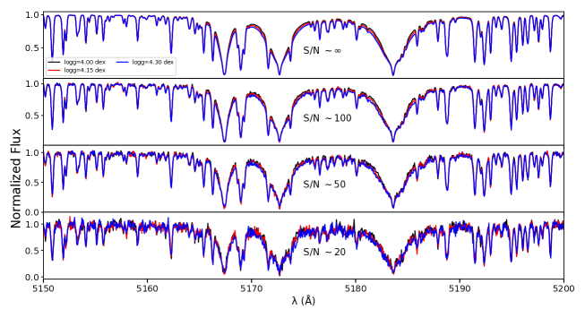
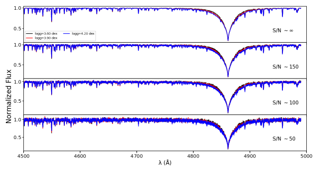
Figures 6 and 7 display the variation in the spectrum profile as a function of $\log g$, fixing all the remaining parameters, for G and A stars, respectively. In Fig. 6, we calculated synthetic spectra for a typical G star with a $T_{\mathrm{eff}}$ of 5 200 K, $[M/H]$ of 0.0 dex, $v\sin i$ of 6 $\mbox{km}\,\mbox{s}^{-1}$ at a resolution of 50 000 and in the wavelength range of 5 000$-$5 400 Å. The only parameter that differs between the 3 spectra is $\log g$, ranging between 4.00 dex and 4.30 dex with a step of 0.15 dex. The upper panel of Fig. 6 displays the normalized flux of the synthetic spectra in the Mg i b triplet region. The flux level in this region is very sensitive to variation in $\log g$. The following panels displays the same spectra for different values of S/N. When no noise is added (panel with S/N$\sim\infty$), the distinction between the 3 spectra is clear but when S/N starts to decrease, the distinction between the noisy spectra becomes harder to detect. This shows that for a S/N in the order of 100, the noisy spectra with $\log g$ of 4.00 and 4.15 dex are very similar and therefore the best corresponding synthetic spectrum in our LDB could have a $\log g$ varying at least 0.15 dex from the correct value. We are not trying to quantify the minimum S/N required for an accurate inversion of $\log g$ as the RSIR is not based on a pixel-to-pixel comparison, but we are showing the effect of our derived standard deviations in $\log g$ on the flux for noisy spectra. Figure 7 displays a similar behaviour for A stars having similar $T_{\mathrm{eff}}$ of 8 500 K, $[M/H]$ of 0.0 dex, $v\sin i$ of 40 $\mbox{km}\,\mbox{s}^{-1}$, at a resolution of 76 000 in the wavelength range of 4 500-5 000 Å. Surface gravity of these spectra ranges between 3.60 and 4.20 dex with a step of 0.30 dex. This figure shows a similar behavior to that of Fig. 6. At a S/N of $\sim$150, the distinction between spectra having a difference of 0.30 dex in $\log g$, becomes hardly noticeable. Figures 6 and 7 also show that the effect of weak metallic lines, on the derivation of $\log g$, becomes negligible as the S/N decreases. The $\log g$ information that these lines contain is mainly lost in the noise.

Fig. 7: Same as for Fig. 6 but for A stars having having [$T_{\mathrm{eff}}$,$\log g$,$[M/H]$,$v\sin i$] of [8 500 K,[3.60,3.90,4.20 dex], 0.0 dex, 40 $\mbox{km}\,\mbox{s}^{-1}$.

6 Discussion and conclusion

RSIR tests for nearly 4 000 synthetic stars of different spectral type and different noise levels showed an improvement over the PCA-based method of Paletou et al. (2015a, b) and Gebran et al. (2016) for the inversion of stellar parameters. Results of Tabs. 2 and 3 and Fig. 4, for FGK and A stars, show that for most of the tests, the $\Lambda$ values of RSIR are lower than nearest neighbor PCA approach. Having a prior information about the star using PCA as a pre-process allows us to narrow down the selection of the optimized reduced databases. This decreases drastically the size of the LDB's. Achieving lower $\Lambda$ with bigger steps helps in decreasing the prohibitive computation time for the construction of databases and the calculations of the PC's. Simulated tests revealed that computation time of RSIR is nearly 1% of that of the process of PCA nearest neighbor approach.

One should be very careful while increasing the size of steps of the parameters because the PCA pre-processing step could deviate drastically from the true inverted values therefore excluding the spectra that actually best describes the observed ones.

Application to observed FGK and A stars reveal a good agreement between the inverted parameters and the ones derived in previous studies. The comparison with Vizier catalog values show an improvement in the derived parameters as compared to the results of Paletou et al. (2015a) and Gebran et al. (2016) for the same stars and LDB's. Surface gravity remains the parameter with the least accuracy. Our derived errors on $\log g$ are in the order of 0.15-0.30 dex. Smarter LDB's should be therefore considered, say, ``adaptive sampling'' (in the parameters under study), taking care with more caution of the flux typical variations at the most sensitive wavelength (sub-)domains, together with the S/N of the observations, instead of the a priori sampling in the parameters. Also, a commonly reported issue with the inversion of stellar parameters using a LDB of synthetic spectra are the so-called ``ambiguities''. This means that two sets of distinct parameters may generate spectra which are beyond ``discernibility''. Given a set of observed spectra to characterize, we could naturally relate that discernibility to their level of S/N. Using a nearest neighbor search PCA-based method, for instance, such a level of S/N can easily be translated into a threshold of distance $\delta_{\rm PCA}$. Then, we can anticipate that, instead of relying on LDB's usually made using a priori sampling in the parameters, a smarter DB should rely on $\delta_{\rm PCA}$ instead. This would imply to set up LDB's for fundamental stellar parameters in a radically different fashion vs. common practices. In the frame of PCA, it would be more relevant to sample properly the full range of parameters with a ``constrained-random'' process ensuring that there are no nearest neighbors closer than $\delta_{\rm PCA}$. Such a ``sieve algorithm'' was first proposed by López Ariste & Casini (2002) in the context of the characterization of magnetic fields from spectropolarimetric data (see also Casini et al. 2013). Another line of development relates to the "structure" of our LDB's. Smarter, or optimal LDB's, using different methods of samplings, should be considered. Such a general issue was already evoked by Bijaoui et al. (2012) for instance.

Available online databases are usually calculated with large steps in $T_{\mathrm{eff}}$ and $\log g$. Our RSIR technique, as it does not require small steps in the LDB, is a good tool to be used with online available synthetic spectra such as the POLLUX database (Palacios et al., 2010) that contains models with temperature ranging between 3 000 and  50 000 K or TLUSTY Non-LTE Line-blanketed Model Atmospheres of O-Type Stars (Lanz & Hubeny, 2003) with $T_{\mathrm{eff}}$ ranging between 27 500 and 55 000 K with 2 500 K steps, and $\log g$ between 3.0 and 4.75 with steps of 0.25 dex. We can also mention the PHOENIX (Husser et al., 2013) models database for stars having $T_{\mathrm{eff}}$$<$12 000 K and the AMBRE (de Laverny et al., 2012) project that contains high-resolution FGKM stellar synthetic spectra.

As an output of the new Gaia Data Release 2, Cropper et al. (2018) describe the Gaia RVS specification as well as the predicted performance at the end of the mission. Gaia RVS will provide us with a large number of spectra in the calcium triplet regime (845$-$872 nm). This triplet is very sensitive to $T_{\mathrm{eff}}$ and $\log g$. The medium resolution (11 500) of the RVS and the small range in wavelength would require LDB smaller than the ones used in our work, leading to a fast application of the RSIR. As we did for the inversion of the S⁴N data in Sec. 5, LDB could be constructed with real observed stars having well known fundamental parameters and with the same resolution. Finally, since RSIR is based on single parameter inversion process, one can also incorporate other parameters at the cost of computing and handling more numerous individual spectra, for example, microturbulence velocity and individual chemical abundances.

Appendix

In this appendix we display the results of the inversion of $\log g$, $[M/H]$, and $v\sin i$. The black line corresponds to the 1-to-1 associated values. The test number, the root mean square error $\Lambda$, and the offset (see Tabs. 2 and 3 for details) are presented.

Fig. 8: Results of the surface gravity inversion for the synthetic A to K stars.

Fig. 9: Results of the metallicity inversion for the synthetic A to K stars.

Fig. 10: Results of projected equatorial velocity inversion for the synthetic A to K stars.

References

- Abolfathi et al. (2018) Abolfathi, B., Aguado, D. S., Aguilar, G., et al. 2018, ApJS, 235, 42
- Allende Prieto et al. (2004) Allende Prieto, C., Barklem, P. S., Lambert, D. L., & Cunha, K. 2004, A & A, 420, 183
- Alves et al. (2015) Alves, S., Benamati, L., Santos, N. C., et al. 2015, MNRAS, 448, 2749
- Bailer-Jones et al. (1998) Bailer-Jones, C. A. L., Irwin, M., & von Hippel, T. 1998, MNRAS, 298, 361
- Bernard-Michel et al. (2007) Bernard-Michel, C. and Douté, S. and Fauvel, M. and Gardes, L. and Girard, S. 2007.[Research Report], INRIA(inria-00187444v2), 91
- Bernard-Michel et al. (2009) Bernard-Michel, C., Douté, S., Fauvel, M., Gardes, L., & Girard, S. 2009, Journal of Geophysical Research (Planets), 114, E06005
- Bijaoui et al. (2012) Bijaoui, A., Recio-Blanco, A., de Laverny, P., & Ordenovic, C. 2012, Statistical Methodology, 9, 55
- Boeche et al. (2018) Boeche, C., Smith, M. C., Grebel, E. K., et al. 2018, AJ, 155, 181
- Buchhave et al. (2012) Buchhave, L. A., Latham, D. W., Johansen, A., et al. 2012, Nature, 486, 375
- Casini et al. (2013) Casini, R., Asensio Ramos, A., Lites, B. W., & López Ariste, A. 2013, APJ, 773, 180
- Chaplin et al. (2014) Chaplin, W. J., Basu, S., Huber, D., et al. 2014, ApJS, 210, 1
- Casey et al. (2016) Casey, A. R., Hogg, D. W., Ness, M., et al. 2016, arXiv:1603.03040
- Castelli & Kurucz (2003) Castelli, F., & Kurucz, R. L. 2003, Modelling of Stellar Atmospheres, 210, A20
- Cayrel & Cayrel (1963) Cayrel, G., & Cayrel, R. 1963, APJ, 137, 431
- Cayrel de Strobel (1969) Cayrel de Strobel, G. 1969, in Proc. of the 3rd Harvard-Smithsonian Conf. on Stellar Atmospheres, ed. O. Gingerich, 35
- Creevey et al. (2013) Creevey, O. L., Thévenin, F., Basu, S., et al. 2013, MNRAS, 431, 2419
- Cropper et al. (2018) Cropper, M., Katz, D., Sartoretti, P., et al. 2018, arXiv:astro-ph/1804.09369
-
Cui et al. (2012)
Cui, X.-Q., Zhao, Y.-H., Chu, Y.-Q., et al. 2012, Research in Astronomy and Astrophysics, 12, 1197.
Data: http://dr5.lamost.org/ - Dieterich et al. (2017) Dieterich, S., Henry, T. J., Benedict, G. F., et al. 2017, American Astronomical Society Meeting Abstracts #229, 229, 240.30
- Fabbro et al. (2018) Fabbro, S., Venn, K. A., O'Briain, T., et al. 2018, MNRAS, 475, 2978
- Gebran et al. (2014) Gebran, M., Monier, R., Royer, F., Lobel, A., & Blomme, R. 2014, Putting A Stars into Context: Evolution, Environment, and Related Stars, 193
- Gebran et al. (2016) Gebran, M., Farah, W., Paletou, F., Monier, R., & Watson, V. 2016, A & A, 589, A83
- Gill et al. (2018) Gill, S., Maxted, P. F. L., & Smalley, B. 2018, arXiv:1801.06106
- Hekker et al. (2013) Hekker, S., Elsworth, Y., Mosser, B., et al. 2013, A & A, 556, A59
- Hubeny & Lanz (1992) Hubeny, I., & Lanz, T. 1992, A & A, 262, 501
- Husser et al. (2013) Husser, T.-O., Wende-von Berg, S., Dreizler, S., et al. 2013, A & A, 553, A6
- Jolliffe (1986) Jolliffe, I. T. 1986, Springer Series in Statistics, Berlin: Springer, 1986
- Katz & Brown (2017) Katz, D., & Brown, A. G. A. 2017, SF2A-2017: Proceedings of the Annual meeting of the French Society of Astronomy and Astrophysics, 259
- Kiefer (1953) Kiefer, J. 1953, Proceedings of the American Mathematical Society, 4, 502
- Kreyszig (2010) Kreyszig, E. , Advanced Engineering Mathematics 2010. (John Wiley & Sons) p .864-871
- Kurucz (1992) Kurucz, R. L. 1992, RMXAA, 23.
- Lanz & Hubeny (2003) Lanz, T., & Hubeny, I. 2003, ApJS, 146, 417
- Latham et al. (2002) Latham, D. W., Stefanik, R. P., Torres, G., et al. 2002, AJ, 124, 1144
- de Laverny et al. (2012) de Laverny, P., Recio-Blanco, A., Worley, C. C., & Plez, B. 2012, A & A, 544, A126
- Li (1991) Li, K.C 1991, Journal of the American Statistical Association, 86, 414, 316
- López Ariste & Casini (2002) López Ariste, A., & Casini, R. 2002, APJ, 575, 529
- McWilliam (1990) McWilliam, A. 1990, ApJS, 74, 1075
- Morris et al. (2018) Morris, M., Kaiser, M. E., Bohlin, R., Kurucz, R., & ACCESS Team 2018, American Astronomical Society Meeting Abstracts #231, 231, #355.27
- Ness et al. (2015) Ness, M., Hogg, D. W., Rix, H.-W., Ho, A. Y. Q., & Zasowski, G. 2015, APJ, 808, 16
- O'Mullane & LSST Data Management Team (2018) O'Mullane, W., & LSST Data Management Team 2018, American Astronomical Society Meeting Abstracts #231, 231, #362.10
- Palacios et al. (2010) Palacios, A., Gebran, M., Josselin, E., et al. 2010, A & A, 516, A13
- Paletou & Zolotukhin (2014) Paletou, F., & Zolotukhin, I. 2014, arXiv:1408.7026
- Paletou et al. (2015a) Paletou, F., Böhm, T., Watson, V., & Trouilhet, J.-F. 2015, A & A, 573, A67
- Paletou et al. (2015b) Paletou, F., Gebran, M., Houdebine, E. R., & Watson, V. 2015, A & A, 580, A78
Perryman et al. (2001)
Perryman, M. A. C., de Boer, K. S., Gilmore, G., et al. 2001, A & A, 369, 339.
Data: https://www.cosmos.esa.int/web/gaia/dr2 - Prugniel & Soubiran (2001) Prugniel, P., & Soubiran, C. 2001, A & A, 369, 1048
- Prugniel et al. (2007) Prugniel, P., Soubiran, C., Koleva, M., & Le Borgne, D. 2007, arXiv:astro-ph/0703658
- Re Fiorentin et al. (2007) Re Fiorentin, P., Bailer-Jones, C. A. L., Lee, Y. S., et al. 2007, A & A, 467, 1373
- Schönrich & Bergemann (2014) Schönrich, R., & Bergemann, M. 2014, MNRAS, 443, 698
- Shevlyakova & Morenthaler (2014) Shevlyakova, M., & Morgenthaler, S. 2014, Statistical Papers, 55, 1
- Smalley (2004) Smalley, B., Zverko, J., Žižňovskỳ, J., Adelman, SJ., and Weiss, WW 2004. The A-Star Puzzle . Proc. IAU Symp. 224 (Cambridge Univ. Press Cambridge).
- Smalley (2005) Smalley, B. 2005, Memorie della Societa Astronomica Italiana Supplementi, 8, 130
- Stoehr et al. (2008) Stoehr, F., White, R., Smith, M., et al. 2008, Astronomical Data Analysis Software and Systems XVII, 394, 505
- Ting et al. (2018) Ting, Y.-S., Conroy, C., Rix, H.-W., & Cargile, P. 2018, arXiv:1804.01530
- Torres et al. (2002) Torres, G., Neuhäuser, R., & Guenther, E. W. 2002, AJ, 123, 1701
- Valenti & Piskunov (1996) Valenti, J. A., & Piskunov, N. 1996, A & AS, 118, 595
- Vogel (2002) C.R. Vogel. Computational methods for inverse problems. Society for Industrial and Applied Mathematics, 2002
- Watson et al. (2017) Watson, V., Trouilhet, J., Paletou, F., & Girard, S. 2017, IEEE International Workshop of Electronics, Control, Measurement, Signals and their Application to Mechatronics (ECMSM)
- Wilkinson et al. (2017) Wilkinson, D. M., Maraston, C., Goddard, D., Thomas, D., & Parikh, T. 2017, MNRAS, 472, 4297
- Xiang et al. (2017) Xiang, M.-S., Liu, X.-W., Shi, J.-R., et al. 2017, MNRAS, 464, 3657