Critical states in Political Trends.
How much reliable is a poll on Twitter? A study by means of the Potts Model

Lucas Nicolao Massimo Ostilli Departamento de Fรญsica, Universidade Federal de Santa Catarina, Florianรณpolis, Brazil Instituto de Fรญsica, Universidade Federal da Bahia, Salvador, Brazil
Abstract

In recent years, Twitter data related to political trends have tentatively been used to make predictions (poll) about several electoral events. Given q๐‘žq candidates for an election and a time-series of Twitts (short messages), one can extract the q๐‘žq mean trends and the qโ€‹(q+1)/2๐‘ž๐‘ž12q(q+1)/2 Twitt-to-Twitt correlations, and look for the statistical models that reproduce these data. On the base of several electoral events and assuming a stationary regime, we find out the following: i) the maximization of the entropy singles out a microscopic model (single-Twitt-level) that coincides with a q๐‘žq-state Potts model having suitable couplings and external fields to be determined via an inverse problem from the two sets of data; ii) correlations decay as 1/Neโ€‹fโ€‹f1subscript๐‘๐‘’๐‘“๐‘“1/N_{eff}, where Neโ€‹fโ€‹fsubscript๐‘๐‘’๐‘“๐‘“N_{eff} is a small fraction of the mean number of Twitts; iii) the simplest statistical models that reproduce these correlations are the multinomial distribution (MD), characterized by q๐‘žq external fields, and the mean-field Potts model (MFP), characterized by one coupling; iv) remarkably, this coupling turns out to be always close to its critical value. This results in a MD or MFP model scenario that discriminates between cases in which polls are reliable and not reliable, respectively. More precisely, predictions based on polls should be avoided whenever the data maps to a MFP because anomalous large fluctuations (if q=2๐‘ž2q=2) or sudden jumps (if qโ‰ฅ3๐‘ž3q\geq 3) in the trends might take place as a result of a second-order or a first-order phase transition of the MFP, respectively.

keywords:
social networks , Potts model , inverse problem
โ€ โ€ journal: Physica A

1 Introduction

Social dynamics is a multidisciplinary subject that, especially in the last two decades, has attracted a strong interest due to an exponential growth of digital data where trends, opinions, and relationships, are nowadays continuously collected and analyzed. In this context, particularly appealing are the Twitter data related to political orientations. In fact, a vast literature in which Twitter messages (Twitts) about politic are analyzed, has already been produced since Twitter creation in 2006 [1, 2, 3, 4, 5, 6, 7, 8]; see also [9] and references therein. In some cases, the analysis of the Twitts collected prior to a particular electoral event in which q๐‘žq candidates compete for the position of president or prime minister, have allowed to predict the actual electoral result, while in some others not, even though a fair statistics is lacking [9]. In these works, the main hypothesis consists in assuming that the set of Twitts collected, say, from day -30 till day -1, is representative of the offline will of vote and contains the information about the winner candidate elected on the day 0, the election day. Each messageโ€™s content is then analyzed and, according to criteria based on specific dictionaries of key words, the Twitt is to be interpreted in favor (mention), or possibly against (sentiment), of one of the q๐‘žq candidates. Any poll, however, is partial and predictions must be taken with care, even when the best criteria for interpreting the messages has been used. The problem with polls is in fact twofold as they are limited in both โ€œspaceโ€ and โ€œtimeโ€: On one side, samples are finite and the statistics suffers from finite size effects, on the other side, samples look only at specific times and, of course, they do not contain any actual information about the future election day. If a system is somehow at a critical point, the above limitations will dramatically affect the predictions even under the hypothesis that the system is approximately in a stationary regime.

In order to justify typical macroscopic patterns observed in social dynamics, several microscopic models have been proposed [10]. So, for example, on the base of elementary laws among neighbors, like replication of opinion, competitions, and external noise, different versions of the Voter model [11], as well as of the Sznajd dynamics [12], have been studied and a large literature produced (see also references in [10]). Despite important progresses in this direction, especially with respect to certain observed universal properties, like the spread of rumor [13], and the vote distribution for electoral events characterized by a large number q๐‘žq of candidates (as in the case of legislators and city councilors elections) [14, 15, 16, 17, 18], most of such studies have remained mainly qualitative (or spectral quantitative), the major problem being the lack of connection between the model-parameters and the actual system-parameters. This issue is in fact one of the most serious one for any microscopic approach to social dynamics, for the couplings and the external fields to which a real social system obeys, if any, depend of an infinite number of different sources out of control, which results in the impossibility of using the model for making predictions.

In this paper, we consider a different perspective. We do not aim at finding the most reliable microscopic model from โ€œfirst-principlesโ€. Rather, we consider effective models which, on the base of a limited number of macroscopic data, are able to incorporate the complex source of the collective behavior, and yet are simply enough to allow for the determination of their actual parameters to be found via an inverse problem, which in turn can reveal surprisingly interesting facts. To track the dynamics of a collection of Twitter users posting Twitts about a specific electoral event with q๐‘žq candidates, in which, at any time t๐‘กt, we have access to the โ€œvolumeโ€ (or number of mentions), i.e., the number of Twitts in favor of a specific candidate and, in some cases also to the โ€œsentimentโ€, i.e., the number of Twitts in favor minus the number of Twitts against a specific candidate, we use a q๐‘žq-state Potts model [19]. The choice of the model is not arbitrary. In fact, as we shall show, a generalized q๐‘žq-state Potts model with suitable couplings and external fields, in principle time-dependent, is the model that maximizes the entropy of a set of data constituted by q๐‘žq mean number of mentions and qโ€‹(q+1)/2๐‘ž๐‘ž12q(q+1)/2 mention-to-mention correlations (more precisely, q๐‘žq auto-correlations, and qโ€‹(qโˆ’1)/2๐‘ž๐‘ž12q(q-1)/2 two-point correlations). In other words, the generalized q๐‘žq-state Potts model is maximally random under the above q+qโ€‹(q+1)/2๐‘ž๐‘ž๐‘ž12q+q(q+1)/2 constrains. Unfortunately (at the present study), we do not have direct access to the mention-to-mention instantaneous correlations (microscopic level, or single-Twitt level). However, under the stationary hypothesis, where no impacting news reach the Twitter network, the system can be considered as isolated. As a consequence, during a stationary regime, any apparent dynamics can be seen as sole due to stochastic fluctuations originating from a time-independent probability distribution and we can derive the macroscopic (or coarse-grained) correlations from the q๐‘žq time series of the mean number of mentions. Quite interestingly, these macroscopic correlations scale always as ๐‘‚(1/Neโ€‹fโ€‹f)๐‘‚1subscript๐‘๐‘’๐‘“๐‘“\mathop{O}(1/N_{eff}), where Neโ€‹fโ€‹fsubscript๐‘๐‘’๐‘“๐‘“N_{eff} is an effective number of messages that can also be calculated from the data and that turns out to be a small fraction of the mean number of messages N๐‘N (where the mean is calculated over the given time interval of observation, ranging from minutes to days). In turn, this implies that the microscopic correlations scale at most as ๐‘‚(1/Neโ€‹fโ€‹f)๐‘‚1subscript๐‘๐‘’๐‘“๐‘“\mathop{O}(1/N_{eff}), i.e., they are effectively mean-field like. Remarkably, by assuming a mean-field Potts model (MFP) characterized by one single coupling J/Neโ€‹fโ€‹f๐ฝsubscript๐‘๐‘’๐‘“๐‘“J/N_{eff}, we find that, in all the electoral events that we have considered, the inverse problem is solved for a J๐ฝJ close to its critical value. However, other mean-field models could work as well. In fact, by comparing in detail the structure of the measured macroscopic correlations with the model macroscopic correlations, we see that, whereas they are both mean-field like (decay as 1/Neโ€‹fโ€‹f1subscript๐‘๐‘’๐‘“๐‘“1/N_{eff}), in some cases the multinomial distribution (MD) turns out to be the best statistical model, while in some others is the MFP. Note that, in the MD case, microscopic correlations are zero, and macroscopic correlations arise only as a consequence of the constraint that the total number of messages is fixed while, in the MFP case, microscopic correlations are present. In both cases, the macroscopic connected correlations functions decay as 1/Neโ€‹fโ€‹f1subscript๐‘๐‘’๐‘“๐‘“1/N_{eff}, but their forms are quite different and allow for a clear distinction between two corresponding scenarios, MD or MFP. Note also that, formally, the MD for q๐‘žq candidates and Neโ€‹fโ€‹fsubscript๐‘๐‘’๐‘“๐‘“N_{eff} messages corresponds to a q๐‘žq-state Potts model with zero coupling and q๐‘žq suitable external fields, while the MFP is characterized by a coupling that scales as 1/Neโ€‹fโ€‹f1subscript๐‘๐‘’๐‘“๐‘“1/N_{eff} and no external field. Clearly, one could look for other mean-field Potts models with more general features able to interpolate between the MD and the MFP, as well as to take into account the scale-free character of the underlying Twitter network [20, 21]. However, the MD and the MFP, which constitute the two simplest and somehow opposite mean-field models, turn out to be able to reproduce well the qโ€‹(q+1)/2๐‘ž๐‘ž12q(q+1)/2 measured macroscopic correlations. In fact, as we shall show, the use of the effective number of messages Neโ€‹fโ€‹fsubscript๐‘๐‘’๐‘“๐‘“N_{eff} allows for taking into account replicas of messages, which can be seen as strong-rigid correlations. This aspect makes the MD and MFP models rather non trivial and effective.

The MD versus MFP scenario is very interesting. Our analysis shows that only in the MD case one can use the Twitts as a poll for predictions. In this case in fact, during an approximate stationary regime, one can simply track the average trends and extrapolate the future election result by making use of standard regression methods. In the case of a MFP model instead, the fact that the model lies in its critical point should alarm the statistician attempting to make predictions about the future electoral result. In fact, for q=2๐‘ž2q=2, where the Potts model is equivalent to the Ising model, at the critical point the system undergoes a second-order phase transition and fluctuations are unbounded in the thermodynamic limit. For qโ‰ฅ2๐‘ž2q\geq 2, instead, the system undergoes a first-order phase transition where fluctuations are bounded but sudden jumps occur. In any case, our analysis shows that, in several electoral events, the system tends to settle itself, for over large time intervals, to its critical point, lying then between the two phases: a liquid/paramagnetic one where each candidate tends to receive, on average, the same percentage of votes, and a crystal/magnetized one where one of the candidates breaks the liquid/paramagnetic symmetry gaining a net advantage over the others. The passages between the two phases appear to be rather unpredictable due to the permanent vicinity to the critical point preventing therefore to make a forecast of the q๐‘žq trends. At least within the context of democratic elections, this scenario of intrinsic unpredictability seems to be due to the controversial spread of political and economic power that takes place among a few symmetrically powerful parties and respective candidates, the strongest of which rarely overcome qโˆผ10similar-to๐‘ž10q\sim 10. Strong candidates are quite able to compete with each other. Typically, a strong candidate publicly speaking at time say, t+1๐‘ก1t+1, has a good chance to fade out the impact of the speech of her/his strong opponents given at prior times t,tโˆ’1,โ€ฆ๐‘ก๐‘ก1โ€ฆt,\leavevmode\nobreak\ t-1,\ldots. This process can result in a continuous rank reversal of the trends that, statistically, translates into a system that remains on the boundary between the two phases. In such a scenario of symmetrically strong candidates, the winner of the election is just the result of a random large fluctuation.

The paper is organized as follows. In Sec. II, we introduce and develop the general inverse problem (IIA) whose formal solution is given in terms of a generalized Potts model having suitable couplings and external fields (IIB), with important simplifications arising in the homogeneous case (IIC) which, in turn, includes the sub-case of zero correlations where the inverse problem is solved by the MD. In Sec. III, we review the MFP in detail (IIIA). Although the MFP can be seen as a particular solution of the inverse problem, for pedagogical reasons we prefer to describe it in a separated section where, in particular, we calculate the connected correlation functions (IIIB). In Sec. IV, we apply the theory to several Twitter data sets of trends (time series of the mean number of mentions, and also sentiment in a specific case). In doing this, we first stress the peculiarities of the MD and MFP models (IVA), then we show how to measure the macroscopic correlations in a stationary regime (IVB), and define the effective number of messages Neโ€‹fโ€‹fsubscript๐‘๐‘’๐‘“๐‘“N_{eff} which provides another interesting information on the tendency of the users to copy each other (IVC). Finally, we apply the theory to several electoral events. At the end, some conclusions are drawn.

2 Inverse Problem in Social Sciences

Here we introduce a general unbiased approach that, in principle, allows to derive the actual system-parameters, although at high computational cost, and also data cost. In fact, it is worth to remind that only certain sets of Twitter data are publicly free. We first illustrate the procedure in a idealized context where we assume that data are known at the user-microscopic level. Next, we shall relax this assumption and make the naive mean-field approximation in order to cope with the incompleteness of the available data and in view of simplicity.

We assume that there exist N๐‘N nodes/users/agents/messages and that each agent owns a status variable ฯƒ๐œŽ\sigma, the โ€œspinโ€, that can take q๐‘žq possible different values labeled as ฯƒ=1,โ€ฆ,q๐œŽ1โ€ฆ๐‘ž\sigma=1,\ldots,q. For example, the state ฯƒ๐œŽ\sigma can represent an opinion on a given topic where only q๐‘žq different answers are possible, or the state can represent the agentโ€™ s preference over a set of q๐‘žq political candidates. The status ฯƒ๐œŽ\sigma must take into account two different tendencies of the spin: a tendency to be influenced by its neighbors, and a tendency to follow a behavior independently from the others. This latter in turn can be either due to an intrinsic tendency of the user to follow her/his believes, or can be due to news and events whose sources are external to the set of the N๐‘N agents. In the framework of equilibrium statistical mechanics, the natural way to model such a system consists in using the q๐‘žq-state Potts model, where the couplings {Ji,j}subscript๐ฝ๐‘–๐‘—\{J_{i,j}\} quantify the tendency of the spins to be influenced by its neighbors, whereas the external fields hisubscriptโ„Ž๐‘–h_{i} quantify the tendency of the spins to follow a behavior independently of the other spins (similar ideas have been applied in [22] for the case q=2๐‘ž2q=2 to analyze the interaction between two communities). The use of the Potts model in a tentative to describe social interactions is perhaps already available in literature but not abundant for q>2๐‘ž2q>2. However, most of the works so far produced in this direction turn out to be quite disconnected from real world phenomena. The concepts themselves of Hamiltonian, coupling, temperature and external field, which are well established physical entities, in social sciences assume a too often abstract meaning and seem to have no direct connection with real data. In this way, the use of statistical mechanics in social science remains a merely pictorial description of the real phenomena under study, with no prediction power. This critics applies also to other tools which traditionally do not belong to statistical mechanics (e.g. community detection algorithms, voter-like models, and so on).

We show here that it is instead possible to introduce in social science a rigorous use of statistical mechanics, where the connection with the real observed data is exact, and where the probabilistic prediction power of statistical mechanics is recovered, though at the expenses of high computational costs as well as expensive data. The following probabilistic method is certainly not original (see for example the same method applied to graph theory to derive the probability distribution in a canonical ensemble of graphs [23]), but it is perhaps new in the present context and highlights several points that are important to our aim.

2.1 The General Problem and its Formal Solution

Let ๐ˆ๐ˆ\bm{\sigma} be the vector of the N๐‘N spin configurations: ๐ˆ=(ฯƒ1,โ€ฆ,ฯƒN)๐ˆsubscript๐œŽ1โ€ฆsubscript๐œŽ๐‘\bm{\sigma}=\left(\sigma_{1},\ldots,\sigma_{N}\right). Let us assume that at any instant t๐‘กt there exists the probability distribution Pโ€‹(๐ˆ;t)๐‘ƒ๐ˆ๐‘กP\left(\bm{\sigma};t\right). Suppose that all we know about the real phenomena under consideration is a set of M๐‘€M independent averages over the distribution Pโ€‹(๐ˆ;t)๐‘ƒ๐ˆ๐‘กP\left(\bm{\sigma};t\right) of certain observables Y(1)โ€‹(๐ˆ),โ€ฆ,Y(M)โ€‹(๐ˆ)superscript๐‘Œ1๐ˆโ€ฆsuperscript๐‘Œ๐‘€๐ˆY^{(1)}\left(\bm{\sigma}\right),\ldots,Y^{(M)}\left(\bm{\sigma}\right) (in the following we shall omit the dependency on t๐‘กt for brevity):

โŸจY(l)โŸฉP=โˆ‘๐ˆPโ€‹(๐ˆ)โ€‹Y(l)โ€‹(๐ˆ),l=1,โ€ฆ,M.formulae-sequencesubscriptdelimited-โŸจโŸฉsuperscript๐‘Œ๐‘™๐‘ƒsubscript๐ˆ๐‘ƒ๐ˆsuperscript๐‘Œ๐‘™๐ˆ๐‘™1โ€ฆ๐‘€\displaystyle\left\langle Y^{(l)}\right\rangle_{P}=\sum_{\bm{\sigma}}P\left(\bm{\sigma}\right)Y^{(l)}\left(\bm{\sigma}\right),\quad l=1,\ldots,M. (1)

We can โ€œderiveโ€ Pโ€‹(๐ˆ)๐‘ƒ๐ˆP\left(\bm{\sigma}\right) as the distribution that maximizes the information entropy Sโ€‹[P]=โˆ’โˆ‘๐ˆPโ€‹(๐ˆ)โ€‹logโก(Pโ€‹(๐ˆ))๐‘†delimited-[]๐‘ƒsubscript๐ˆ๐‘ƒ๐ˆ๐‘ƒ๐ˆS[P]=-\sum_{\bm{\sigma}}P\left(\bm{\sigma}\right)\log\left(P\left(\bm{\sigma}\right)\right) under the M๐‘€M constraints (1). In other words, we have to find the distribution Qโ€‹(๐ˆ)๐‘„๐ˆQ\left(\bm{\sigma}\right) that maximizes the following functional

S~โ€‹[Pโ€ฒ,ฮป(1),โ€ฆ,ฮป(M),ฮผ]=Sโ€‹[Pโ€ฒ]~๐‘†superscript๐‘ƒโ€ฒsuperscript๐œ†1โ€ฆsuperscript๐œ†๐‘€๐œ‡๐‘†delimited-[]superscript๐‘ƒโ€ฒ\displaystyle\widetilde{S}[P^{\prime},\lambda^{(1)},\ldots,\lambda^{(M)},\mu]=S[P^{\prime}]
+โˆ‘l=1Mฮป(1)โ€‹(โŸจY(l)โŸฉPโ€ฒโˆ’โŸจY(l)โŸฉP)+ฮผโ€‹(โˆ‘๐ˆPโ€ฒโ€‹(๐ˆ)โˆ’1),superscriptsubscript๐‘™1๐‘€superscript๐œ†1subscriptdelimited-โŸจโŸฉsuperscript๐‘Œ๐‘™superscript๐‘ƒโ€ฒsubscriptdelimited-โŸจโŸฉsuperscript๐‘Œ๐‘™๐‘ƒ๐œ‡subscript๐ˆsuperscript๐‘ƒโ€ฒ๐ˆ1\displaystyle+\sum_{l=1}^{M}\lambda^{(1)}\left(\left\langle Y^{(l)}\right\rangle_{P^{\prime}}-\left\langle Y^{(l)}\right\rangle_{P}\right)+\mu\left(\sum_{\bm{\sigma}}P^{\prime}\left(\bm{\sigma}\right)-1\right), (2)

where Pโ€ฒsuperscript๐‘ƒโ€ฒP^{\prime} is a trial probability distribution. The maximum of S~โ€‹[Pโ€ฒ,ฮป(1),โ€ฆ,ฮป(M),ฮผ]~๐‘†superscript๐‘ƒโ€ฒsuperscript๐œ†1โ€ฆsuperscript๐œ†๐‘€๐œ‡\widetilde{S}[P^{\prime},\lambda^{(1)},\ldots,\lambda^{(M)},\mu] must be found with respect to Pโ€ฒsuperscript๐‘ƒโ€ฒP^{\prime} and the M+1๐‘€1M+1 Lagrangian multipliers, ฮป(1),โ€ฆ,ฮป(M)superscript๐œ†1โ€ฆsuperscript๐œ†๐‘€\lambda^{(1)},\ldots,\lambda^{(M)} and ฮผ๐œ‡\mu. The latter Lagrangian multiplier ensures the normalization of Pโ€ฒsuperscript๐‘ƒโ€ฒP^{\prime} while the others ensure that the M๐‘€M constraints (1) are satisfied. The general formal solution of the above problem is the following Gibbs-like distribution

Qโ€‹(๐ˆ)=eโˆ’Hโ€‹(๐ˆ)Z,Z=โˆ‘๐ˆeโˆ’Hโ€‹(๐ˆ)formulae-sequence๐‘„๐ˆsuperscript๐‘’๐ป๐ˆ๐‘๐‘subscript๐ˆsuperscript๐‘’๐ป๐ˆ\displaystyle Q\left(\bm{\sigma}\right)=\frac{e^{-H\left(\bm{\sigma}\right)}}{Z},\qquad Z=\sum_{\bm{\sigma}}e^{-H\left(\bm{\sigma}\right)} (3)

where

Hโ€‹(๐ˆ)=โˆ‘l=1Mฮป(l)โ€‹Y(l)โ€‹(๐ˆ),๐ป๐ˆsuperscriptsubscript๐‘™1๐‘€superscript๐œ†๐‘™superscript๐‘Œ๐‘™๐ˆ\displaystyle H\left(\bm{\sigma}\right)=\sum_{l=1}^{M}\lambda^{(l)}Y^{(l)}\left(\bm{\sigma}\right), (4)

and the M๐‘€M Lagrangian multipliers ฮป(1),โ€ฆ,ฮป(M)superscript๐œ†1โ€ฆsuperscript๐œ†๐‘€\lambda^{(1)},\ldots,\lambda^{(M)} solve the following system of Eqs.

โŸจY(l)โŸฉP=โŸจY(l)โŸฉQor,moreโ€‹explicitlysubscriptdelimited-โŸจโŸฉsuperscript๐‘Œ๐‘™๐‘ƒsubscriptdelimited-โŸจโŸฉsuperscript๐‘Œ๐‘™๐‘„ormoreexplicitly\displaystyle\left\langle Y^{(l)}\right\rangle_{P}=\left\langle Y^{(l)}\right\rangle_{Q}\quad\mathrm{or,\leavevmode\nobreak\ more\leavevmode\nobreak\ explicitly}
โŸจY(l)โŸฉP=โˆ‘๐ˆeโˆ’Hโ€‹(๐ˆ)โ€‹Y(l)โ€‹(๐ˆ)Z,l=1,โ€ฆ,M.formulae-sequencesubscriptdelimited-โŸจโŸฉsuperscript๐‘Œ๐‘™๐‘ƒsubscript๐ˆsuperscript๐‘’๐ป๐ˆsuperscript๐‘Œ๐‘™๐ˆ๐‘๐‘™1โ€ฆ๐‘€\displaystyle\left\langle Y^{(l)}\right\rangle_{P}=\sum_{\bm{\sigma}}\frac{e^{-H\left(\bm{\sigma}\right)}Y^{(l)}\left(\bm{\sigma}\right)}{Z},\quad l=1,\ldots,M. (5)

Notice that the normalization condition of Q๐‘„Q is automatically satisfied (ฮผ๐œ‡\mu is absorbed in Z๐‘Z). We stress that, in general, Q๐‘„Q does not coincide with the target unknown distribution P๐‘ƒP. In fact, only in the limit of an infinite number of independent averages we can have the equality between the two distributions (formally, Qโ†’Pโ†’๐‘„๐‘ƒQ\to P for Mโ†’โˆžโ†’๐‘€M\to\infty). For M๐‘€M finite, Q๐‘„Q is simply the distribution that, under the M๐‘€M constrains (1), is maximally random with respect to the distribution P๐‘ƒP.

More precisely, the use of Shannonโ€™ s entropy ensures that: i) Q๐‘„Q is maximally random under the M๐‘€M constrains (there are in principle other functionals that satisfy the same requirement, like Rรฉnyiโ€™ s and Tsallis entropy), ii) if for some data we have, for example, โŸจฯƒ1โ€‹ฯƒ2โŸฉP=โŸจฯƒ1โŸฉPโ€‹โŸจฯƒ2โŸฉPsubscriptdelimited-โŸจโŸฉsubscript๐œŽ1subscript๐œŽ2๐‘ƒsubscriptdelimited-โŸจโŸฉsubscript๐œŽ1๐‘ƒsubscriptdelimited-โŸจโŸฉsubscript๐œŽ2๐‘ƒ\left\langle\sigma_{1}\sigma_{2}\right\rangle_{P}=\left\langle\sigma_{1}\right\rangle_{P}\left\langle\sigma_{2}\right\rangle_{P}, this means that Pโ€‹(ฯƒ1,ฯƒ2)=Pโ€‹(ฯƒ1)โ€‹Pโ€‹(ฯƒ2)๐‘ƒsubscript๐œŽ1subscript๐œŽ2๐‘ƒsubscript๐œŽ1๐‘ƒsubscript๐œŽ2P(\sigma_{1},\sigma_{2})=P(\sigma_{1})P(\sigma_{2}), a property which is consistent only with an additive (and then extensive) entropy, like the Shannonโ€™ s or the Rรฉnyiโ€™ s entropy, iii) the chain rule for the conditional probability, Hโ€‹(ฯƒ1|ฯƒ2)=Hโ€‹(ฯƒ1,ฯƒ2)โˆ’Hโ€‹(ฯƒ2)๐ปconditionalsubscript๐œŽ1subscript๐œŽ2๐ปsubscript๐œŽ1subscript๐œŽ2๐ปsubscript๐œŽ2H(\sigma_{1}|\sigma_{2})=H(\sigma_{1},\sigma_{2})-H(\sigma_{2}) (which is a natural requirement in information theory), is satisfied only by the Shannonโ€™s entropy.

2.2 Most general means and correlations

Let us now consider a system of N๐‘N agents ฯƒ1,โ€ฆ,ฯƒNsubscript๐œŽ1โ€ฆsubscript๐œŽ๐‘\sigma_{1},\ldots,\sigma_{N} where, at any instant, ฯƒisubscript๐œŽ๐‘–\sigma_{i} can take one over q๐‘žq possible values 1,โ€ฆ,q1โ€ฆ๐‘ž1,\ldots,q. We assume that, at any instant t๐‘กt, we have the following independent dataย 111 The sets of data xยฏฯƒ;isubscriptยฏ๐‘ฅ๐œŽ๐‘–\overline{x}_{\sigma;i} are of course not independent since โˆ‘ฯƒxยฏฯƒ;i=1subscript๐œŽsubscriptยฏ๐‘ฅ๐œŽ๐‘–1\sum_{\sigma}\overline{x}_{\sigma;i}=1 for any i๐‘–i. Formally, we can deal with this issue by making use of another Lagrangian multiplier ฮผโ€ฒsuperscript๐œ‡โ€ฒ\mu^{\prime} to be used in Eq. (2.1) that takes into account this constrain. However, it is easy to see that ฮผโ€ฒโ€‹Nsuperscript๐œ‡โ€ฒ๐‘\mu^{\prime}N can be absorbed in ฮผ๐œ‡\mu with no effect in the final result for Qโ€‹(๐ˆ)๐‘„๐ˆQ(\bm{\sigma}), Eqs. (3-2.1) being the same. :

xยฏฯƒ;iโ‰กโŸจฮดโ€‹(ฯƒi,ฯƒ)โŸฉP,i=1,โ€ฆ,N,ฯƒ=1,โ€ฆ,q,formulae-sequencesubscriptยฏ๐‘ฅ๐œŽ๐‘–subscriptdelimited-โŸจโŸฉ๐›ฟsubscript๐œŽ๐‘–๐œŽ๐‘ƒformulae-sequence๐‘–1โ€ฆ๐‘๐œŽ1โ€ฆ๐‘ž\displaystyle\overline{x}_{\sigma;i}\equiv\left\langle\delta(\sigma_{i},\sigma)\right\rangle_{P},\quad i=1,\ldots,N,\quad\sigma=1,\ldots,q, (6)

and

Cฯƒ,ฯƒโ€ฒ;i,jsubscript๐ถ๐œŽsuperscript๐œŽโ€ฒ๐‘–๐‘—\displaystyle C_{\sigma,\sigma^{\prime};i,j} โ‰ก\displaystyle\equiv โŸจฮดโ€‹(ฯƒi,ฯƒ)โ€‹ฮดโ€‹(ฯƒj,ฯƒโ€ฒ)โŸฉP,subscriptdelimited-โŸจโŸฉ๐›ฟsubscript๐œŽ๐‘–๐œŽ๐›ฟsubscript๐œŽ๐‘—superscript๐œŽโ€ฒ๐‘ƒ\displaystyle\left\langle\delta(\sigma_{i},\sigma)\delta(\sigma_{j},\sigma^{\prime})\right\rangle_{P}, (7)
i,j=1,โ€ฆ,N,ฯƒ,ฯƒโ€ฒ=1,โ€ฆ,q.formulae-sequence๐‘–๐‘—1โ€ฆ๐‘๐œŽsuperscript๐œŽโ€ฒ1โ€ฆ๐‘ž\displaystyle i,j=1,\ldots,N,\quad\sigma,\sigma^{\prime}=1,\ldots,q.

Notice that in defining the correlation Cฯƒ,ฯƒโ€ฒ;i,jsubscript๐ถ๐œŽsuperscript๐œŽโ€ฒ๐‘–๐‘—C_{\sigma,\sigma^{\prime};i,j}, we have imposed iโ‰ j๐‘–๐‘—i\neq j since the information corresponding to i=j๐‘–๐‘—i=j is already contained in the data of xยฏฯƒ;isubscriptยฏ๐‘ฅ๐œŽ๐‘–\overline{x}_{\sigma;i}. According to Eqs. (3)-(2.1), we have the following general Gibbs-Boltzmann form

Qโ€‹(๐ˆ)=eโˆ’Hโ€‹(๐ˆ)Z,Z=โˆ‘๐ˆeโˆ’Hโ€‹(๐ˆ)formulae-sequence๐‘„๐ˆsuperscript๐‘’๐ป๐ˆ๐‘๐‘subscript๐ˆsuperscript๐‘’๐ป๐ˆ\displaystyle Q(\bm{\sigma})=\frac{e^{-H\left(\bm{\sigma}\right)}}{Z},\qquad Z=\sum_{\bm{\sigma}}e^{-H\left(\bm{\sigma}\right)} (8)

where

Hโ€‹(๐ˆ)๐ป๐ˆ\displaystyle H(\bm{\sigma}) =\displaystyle= โˆ’โˆ‘iโˆ‘ฯƒhฯƒ;iโ€‹ฮดโ€‹(ฯƒi,ฯƒ)subscript๐‘–subscript๐œŽsubscriptโ„Ž๐œŽ๐‘–๐›ฟsubscript๐œŽ๐‘–๐œŽ\displaystyle-\sum_{i}\sum_{\sigma}h_{\sigma;i}\delta(\sigma_{i},\sigma) (9)
โˆ’โˆ‘i<jโˆ‘ฯƒ,ฯƒโ€ฒJฯƒ,ฯƒโ€ฒ;i,jโ€‹ฮดโ€‹(ฯƒi,ฯƒ)โ€‹ฮดโ€‹(ฯƒโ€ฒ,ฯƒj),subscript๐‘–๐‘—subscript๐œŽsuperscript๐œŽโ€ฒsubscript๐ฝ๐œŽsuperscript๐œŽโ€ฒ๐‘–๐‘—๐›ฟsubscript๐œŽ๐‘–๐œŽ๐›ฟsuperscript๐œŽโ€ฒsubscript๐œŽ๐‘—\displaystyle-\sum_{i<j}\sum_{\sigma,\sigma^{\prime}}J_{\sigma,\sigma^{\prime};i,j}\delta(\sigma_{i},\sigma)\delta(\sigma^{\prime},\sigma_{j}),

where hฯƒ;isubscriptโ„Ž๐œŽ๐‘–h_{\sigma;i} and Jฯƒ,ฯƒโ€ฒ;i,jsubscript๐ฝ๐œŽsuperscript๐œŽโ€ฒ๐‘–๐‘—J_{\sigma,\sigma^{\prime};i,j} are two sets of adimensional parameters, called external fields and couplings, which must satisfy the constrains (6) and (7)

โˆ‘๐ˆโ€ฒeโˆ’Hโ€‹(๐ˆโ€ฒ)โ€‹ฮดฯƒiโ€ฒ,ฯƒZ=xยฏฯƒ;i,j=1,โ€ฆ,N,ฯƒ=1,โ€ฆ,q,formulae-sequencesubscriptsuperscript๐ˆโ€ฒsuperscript๐‘’๐ปsuperscript๐ˆโ€ฒsubscript๐›ฟsuperscriptsubscript๐œŽ๐‘–โ€ฒ๐œŽ๐‘subscriptยฏ๐‘ฅ๐œŽ๐‘–formulae-sequence๐‘—1โ€ฆ๐‘๐œŽ1โ€ฆ๐‘ž\displaystyle\sum_{\bm{\sigma}^{\prime}}\frac{e^{-H\left(\bm{\sigma}^{\prime}\right)}\delta_{{\sigma}_{i}^{\prime},\sigma}}{Z}=\overline{x}_{\sigma;i},\quad j=1,\ldots,N,\quad\sigma=1,\ldots,q, (10)

and

โˆ‘๐ˆโ€ฒeโˆ’Hโ€‹(๐ˆโ€ฒ)โ€‹ฮดโ€‹(ฯƒiโ€ฒ,ฯƒ)โ€‹ฮดโ€‹(ฯƒjโ€ฒ,ฯƒโ€ฒ)Z=Cฯƒ,ฯƒโ€ฒ;i,j,subscriptsuperscript๐ˆโ€ฒsuperscript๐‘’๐ปsuperscript๐ˆโ€ฒ๐›ฟsuperscriptsubscript๐œŽ๐‘–โ€ฒ๐œŽ๐›ฟsuperscriptsubscript๐œŽ๐‘—โ€ฒsuperscript๐œŽโ€ฒ๐‘subscript๐ถ๐œŽsuperscript๐œŽโ€ฒ๐‘–๐‘—\displaystyle\sum_{\bm{\sigma}^{\prime}}\frac{e^{-H\left(\bm{\sigma}^{\prime}\right)}\delta(\sigma_{i}^{\prime},\sigma)\delta(\sigma_{j}^{\prime},\sigma^{\prime})}{Z}=C_{\sigma,\sigma^{\prime};i,j},
i<j,i,j=1,โ€ฆ,N,ฯƒ.ฯƒโ€ฒ=1,โ€ฆ,q.formulae-sequenceformulae-sequence๐‘–๐‘—๐‘–๐‘—1โ€ฆ๐‘๐œŽsuperscript๐œŽโ€ฒ1โ€ฆ๐‘ž\displaystyle\quad i<j,\quad i,j=1,\ldots,N,\quad\sigma.\sigma^{\prime}=1,\ldots,q. (11)

Eqs. (10) and (2.2) establish our inverse problem: having the sets of the means xยฏฯƒ;isubscriptยฏ๐‘ฅ๐œŽ๐‘–\overline{x}_{\sigma;i} and the set of the correlations Cฯƒ,ฯƒโ€ฒ;i,jsubscript๐ถ๐œŽsuperscript๐œŽโ€ฒ๐‘–๐‘—C_{\sigma,\sigma^{\prime};i,j}, we have the necessary and sufficient conditions to find, at least numerically, the set of the external fields hฯƒ;isubscriptโ„Ž๐œŽ๐‘–h_{\sigma;i}, and the set of the couplings Jฯƒ,ฯƒโ€ฒ;i,jsubscript๐ฝ๐œŽsuperscript๐œŽโ€ฒ๐‘–๐‘—J_{\sigma,\sigma^{\prime};i,j}.

2.3 Homogeneous case

Above, we have discussed a very general case in which userโ€™ s orientation and user-user correlations depend both on the user and on the orientation. However, in a sufficiently large system, we expect the following homogeneity to take place for the two sets of data:

xยฏฯƒ;i=xยฏฯƒ,i=1,โ€ฆ,N,ฯƒ=1,โ€ฆ,q,formulae-sequencesubscriptยฏ๐‘ฅ๐œŽ๐‘–subscriptยฏ๐‘ฅ๐œŽformulae-sequence๐‘–1โ€ฆ๐‘๐œŽ1โ€ฆ๐‘ž\displaystyle\overline{x}_{\sigma;i}=\overline{x}_{\sigma},\qquad i=1,\ldots,N,\qquad\sigma=1,\ldots,q, (12)

and

Cฯƒ,ฯƒโ€ฒ;i,j=Cฯƒ,ฯƒโ€ฒ,i<j,i,j=1,โ€ฆ,N,ฯƒ,ฯƒโ€ฒ=1,โ€ฆ,q.formulae-sequencesubscript๐ถ๐œŽsuperscript๐œŽโ€ฒ๐‘–๐‘—subscript๐ถ๐œŽsuperscript๐œŽโ€ฒformulae-sequence๐‘–๐‘—๐‘–formulae-sequence๐‘—1โ€ฆ๐‘๐œŽsuperscript๐œŽโ€ฒ1โ€ฆ๐‘ž\displaystyle C_{\sigma,\sigma^{\prime};i,j}=C_{\sigma,\sigma^{\prime}},\leavevmode\nobreak\ i<j,\quad i,j=1,\ldots,N,\quad\sigma,\sigma^{\prime}=1,\ldots,q. (13)

The meanings of xยฏฯƒsubscriptยฏ๐‘ฅ๐œŽ\overline{x}_{\sigma} and Cฯƒ,ฯƒโ€ฒsubscript๐ถ๐œŽsuperscript๐œŽโ€ฒC_{\sigma,\sigma^{\prime}} are

xยฏฯƒ=Prob.(forโ€‹aโ€‹randomlyโ€‹chosenโ€‹userโ€‹toโ€‹haveโ€‹statusโ€‹ฯƒ),formulae-sequencesubscriptยฏ๐‘ฅ๐œŽProbforarandomlychosenusertohavestatus๐œŽ\displaystyle\overline{x}_{\sigma}=\mathrm{Prob.}\left(\mathrm{for\leavevmode\nobreak\ a\leavevmode\nobreak\ randomly\leavevmode\nobreak\ chosen\leavevmode\nobreak\ user\leavevmode\nobreak\ to\leavevmode\nobreak\ have\leavevmode\nobreak\ status\leavevmode\nobreak\ }\sigma\right), (14)
Cฯƒ,ฯƒโ€ฒsubscript๐ถ๐œŽsuperscript๐œŽโ€ฒ\displaystyle C_{\sigma,\sigma^{\prime}} =\displaystyle= Prob.(fortworandomlychosenusers\displaystyle\mathrm{Prob.}\left(\mathrm{for\leavevmode\nobreak\ two\leavevmode\nobreak\ randomly\leavevmode\nobreak\ chosen\leavevmode\nobreak\ users}\right. (15)
tohavestatusฯƒandฯƒโ€ฒ).\displaystyle\left.\mathrm{\leavevmode\nobreak\ \leavevmode\nobreak\ \leavevmode\nobreak\ \leavevmode\nobreak\ \leavevmode\nobreak\ \leavevmode\nobreak\ \leavevmode\nobreak\ \leavevmode\nobreak\ \leavevmode\nobreak\ \leavevmode\nobreak\ \leavevmode\nobreak\ to\leavevmode\nobreak\ have\leavevmode\nobreak\ status\leavevmode\nobreak\ }\sigma\leavevmode\nobreak\ \mathrm{and\leavevmode\nobreak\ }\sigma^{\prime}\right).

In turn, Eqs. (12) and (13) imply

xยฏฯƒ=โŸจโˆ‘iฮดโ€‹(ฯƒi,ฯƒ)โŸฉPN=โŸจxฯƒโŸฉP,ฯƒ=1,โ€ฆ,q,formulae-sequencesubscriptยฏ๐‘ฅ๐œŽsubscriptdelimited-โŸจโŸฉsubscript๐‘–๐›ฟsubscript๐œŽ๐‘–๐œŽ๐‘ƒ๐‘subscriptdelimited-โŸจโŸฉsubscript๐‘ฅ๐œŽ๐‘ƒ๐œŽ1โ€ฆ๐‘ž\displaystyle\overline{x}_{\sigma}=\frac{\left\langle\sum_{i}\delta(\sigma_{i},\sigma)\right\rangle_{P}}{N}=\left\langle x_{\sigma}\right\rangle_{P},\qquad\sigma=1,\ldots,q, (16)

and

Cฯƒ,ฯƒโ€ฒ=2โ€‹โŸจโˆ‘i<jฮดโ€‹(ฯƒi,ฯƒ)โ€‹ฮดโ€‹(ฯƒj,ฯƒโ€ฒ)โŸฉPNโ€‹(Nโˆ’1)=subscript๐ถ๐œŽsuperscript๐œŽโ€ฒ2subscriptdelimited-โŸจโŸฉsubscript๐‘–๐‘—๐›ฟsubscript๐œŽ๐‘–๐œŽ๐›ฟsubscript๐œŽ๐‘—superscript๐œŽโ€ฒ๐‘ƒ๐‘๐‘1absent\displaystyle C_{\sigma,\sigma^{\prime}}=\frac{2\left\langle\sum_{i<j}\delta(\sigma_{i},\sigma)\delta(\sigma_{j},\sigma^{\prime})\right\rangle_{P}}{N(N-1)}=
โŸจxฯƒโ€‹xฯƒโ€ฒโŸฉPโˆ’ฮดฯƒ,ฯƒโ€ฒNโ€‹โŸจxฯƒโŸฉP,ฯƒ,ฯƒโ€ฒ=1,โ€ฆ,q,formulae-sequencesubscriptdelimited-โŸจโŸฉsubscript๐‘ฅ๐œŽsubscript๐‘ฅsuperscript๐œŽโ€ฒ๐‘ƒsubscript๐›ฟ๐œŽsuperscript๐œŽโ€ฒ๐‘subscriptdelimited-โŸจโŸฉsubscript๐‘ฅ๐œŽ๐‘ƒ๐œŽsuperscript๐œŽโ€ฒ1โ€ฆ๐‘ž\displaystyle\left\langle x_{\sigma}x_{\sigma^{\prime}}\right\rangle_{P}-\frac{\delta_{\sigma,\sigma^{\prime}}}{N}\left\langle x_{\sigma}\right\rangle_{P},\qquad\sigma,\sigma^{\prime}=1,\ldots,q, (17)

where we have used Nโˆ’1โ‰ƒNsimilar-to-or-equals๐‘1๐‘N-1\simeq N, and introduced the โ€œfrequencyโ€ random variable

xฯƒ=1Nโ€‹โˆ‘iฮดโ€‹(ฯƒi,ฯƒ).subscript๐‘ฅ๐œŽ1๐‘subscript๐‘–๐›ฟsubscript๐œŽ๐‘–๐œŽ\displaystyle x_{\sigma}=\frac{1}{N}\sum_{i}\delta(\sigma_{i},\sigma). (18)

Eqs. (16) and (2.3) are important because they are expressed in terms of the random variables xฯƒsubscript๐‘ฅ๐œŽx_{\sigma}โ€™s which constitute the only information available to us.

The homogeneous assumptions (12) and (13) imply that the Hamiltonian takes the following form

Hโ€‹(๐ˆ)๐ป๐ˆ\displaystyle H(\bm{\sigma}) =\displaystyle= โˆ’โˆ‘ฯƒ,ฯƒโ€ฒJฯƒ,ฯƒโ€ฒโ€‹โˆ‘i<jฮดโ€‹(ฯƒi,ฯƒ)โ€‹ฮดโ€‹(ฯƒj,ฯƒโ€ฒ)subscript๐œŽsuperscript๐œŽโ€ฒsubscript๐ฝ๐œŽsuperscript๐œŽโ€ฒsubscript๐‘–๐‘—๐›ฟsubscript๐œŽ๐‘–๐œŽ๐›ฟsubscript๐œŽ๐‘—superscript๐œŽโ€ฒ\displaystyle-\sum_{\sigma,\sigma^{\prime}}J_{\sigma,\sigma^{\prime}}\sum_{i<j}\delta(\sigma_{i},\sigma)\delta(\sigma_{j},\sigma^{\prime}) (19)
โˆ’โˆ‘ฯƒhฯƒโ€‹โˆ‘iฮดโ€‹(ฯƒi,ฯƒ),subscript๐œŽsubscriptโ„Ž๐œŽsubscript๐‘–๐›ฟsubscript๐œŽ๐‘–๐œŽ\displaystyle-\sum_{\sigma}h_{\sigma}\sum_{i}\delta(\sigma_{i},\sigma),

where the sets of external fields and couplings must satisfy

โˆ‘๐ˆโ€ฒeโˆ’Hโ€‹(๐ˆโ€ฒ)โ€‹ฮดฯƒ1โ€ฒ,ฯƒZ=xยฏฯƒ,ฯƒ=1,โ€ฆ,q,formulae-sequencesubscriptsuperscript๐ˆโ€ฒsuperscript๐‘’๐ปsuperscript๐ˆโ€ฒsubscript๐›ฟsuperscriptsubscript๐œŽ1โ€ฒ๐œŽ๐‘subscriptยฏ๐‘ฅ๐œŽ๐œŽ1โ€ฆ๐‘ž\displaystyle\sum_{\bm{\sigma}^{\prime}}\frac{e^{-H\left(\bm{\sigma}^{\prime}\right)}\delta_{{\sigma}_{1}^{\prime},\sigma}}{Z}=\overline{x}_{\sigma},\qquad\sigma=1,\ldots,q, (20)

and

โˆ‘๐ˆโ€ฒโ€ฒeโˆ’Hโ€‹(๐ˆโ€ฒโ€ฒ)โ€‹ฮดฯƒ1โ€ฒโ€ฒ,ฯƒโ€‹ฮดฯƒ2โ€ฒโ€ฒ,ฯƒโ€ฒZ=Cฯƒ,ฯƒโ€ฒ,ฯƒ,ฯƒโ€ฒ=1,โ€ฆโ€‹q.formulae-sequencesubscriptsuperscript๐ˆโ€ฒโ€ฒsuperscript๐‘’๐ปsuperscript๐ˆโ€ฒโ€ฒsubscript๐›ฟsuperscriptsubscript๐œŽ1โ€ฒโ€ฒ๐œŽsubscript๐›ฟsuperscriptsubscript๐œŽ2โ€ฒโ€ฒsuperscript๐œŽโ€ฒ๐‘subscript๐ถ๐œŽsuperscript๐œŽโ€ฒ๐œŽsuperscript๐œŽโ€ฒ1โ€ฆ๐‘ž\displaystyle\sum_{\bm{\sigma}^{\prime\prime}}\frac{e^{-H\left(\bm{\sigma}^{\prime\prime}\right)}\delta_{\sigma_{1}^{\prime\prime},\sigma}\delta_{\sigma_{2}^{\prime\prime},\sigma^{\prime}}}{Z}=C_{\sigma,\sigma^{\prime}},\qquad\sigma,\sigma^{\prime}=1,\ldots q. (21)

It is understood that, in the homogeneous case, we are free to measure the correlations by means of Eqs. (7) to be used in the inverse problem via Eq. (21), or by means of โŸจxฯƒโ€‹xฯƒโ€ฒโŸฉPsubscriptdelimited-โŸจโŸฉsubscript๐‘ฅ๐œŽsubscript๐‘ฅsuperscript๐œŽโ€ฒ๐‘ƒ\left\langle x_{\sigma}x_{\sigma^{\prime}}\right\rangle_{P} via

โˆ‘๐ˆโ€ฒโ€ฒeโˆ’Hโ€‹(๐ˆโ€ฒโ€ฒ)โ€‹xฯƒโ€‹xฯƒโ€ฒZ=โŸจxฯƒโ€‹xฯƒโ€ฒโŸฉP,ฯƒ,ฯƒโ€ฒ=1,โ€ฆโ€‹q.formulae-sequencesubscriptsuperscript๐ˆโ€ฒโ€ฒsuperscript๐‘’๐ปsuperscript๐ˆโ€ฒโ€ฒsubscript๐‘ฅ๐œŽsubscript๐‘ฅsuperscript๐œŽโ€ฒ๐‘subscriptdelimited-โŸจโŸฉsubscript๐‘ฅ๐œŽsubscript๐‘ฅsuperscript๐œŽโ€ฒ๐‘ƒ๐œŽsuperscript๐œŽโ€ฒ1โ€ฆ๐‘ž\displaystyle\sum_{\bm{\sigma}^{\prime\prime}}\frac{e^{-H\left(\bm{\sigma}^{\prime\prime}\right)}x_{\sigma}x_{\sigma^{\prime}}}{Z}=\left\langle x_{\sigma}x_{\sigma^{\prime}}\right\rangle_{P},\qquad\sigma,\sigma^{\prime}=1,\ldots q. (22)

and similarly for the connected correlation functions.

Homogeneous uncorrelated case - Multinomial Distribution

This case applies when the ฯƒisubscript๐œŽ๐‘–\sigma_{i}โ€™s are independent and uniformly distributed random variables. As a consequence, trivial correlations exist only for the frequency random variable xฯƒsubscript๐‘ฅ๐œŽx_{\sigma}โ€™s, Eqs. (18). In fact, due to the constraint โˆ‘ฯƒxฯƒ=1subscript๐œŽsubscript๐‘ฅ๐œŽ1\sum_{\sigma}x_{\sigma}=1, it is easy to see that

โŸจxฯƒโ€‹xฯƒโ€ฒโŸฉโˆ’โŸจxฯƒโŸฉโ€‹โŸจxฯƒโ€ฒโŸฉ=1Nโ€‹[xยฏฯƒโ€‹ฮดฯƒ,ฯƒโ€ฒโˆ’xยฏฯƒโ€‹xยฏฯƒโ€ฒ],delimited-โŸจโŸฉsubscript๐‘ฅ๐œŽsubscript๐‘ฅsuperscript๐œŽโ€ฒdelimited-โŸจโŸฉsubscript๐‘ฅ๐œŽdelimited-โŸจโŸฉsubscript๐‘ฅsuperscript๐œŽโ€ฒ1๐‘delimited-[]subscriptยฏ๐‘ฅ๐œŽsubscript๐›ฟ๐œŽsuperscript๐œŽโ€ฒsubscriptยฏ๐‘ฅ๐œŽsubscriptยฏ๐‘ฅsuperscript๐œŽโ€ฒ\displaystyle\langle x_{\sigma}x_{\sigma^{\prime}}\rangle-\langle x_{\sigma}\rangle\langle x_{\sigma^{\prime}}\rangle=\frac{1}{N}\left[\overline{x}_{\sigma}\delta_{\sigma,\sigma^{\prime}}-\overline{x}_{\sigma}\overline{x}_{\sigma^{\prime}}\right], (23)

and the probability distribution for the xฯƒsubscript๐‘ฅ๐œŽx_{\sigma}โ€™s, Qโ€‹(๐ˆ)๐‘„๐ˆQ(\bm{\sigma}), turns to be the multinomial distribution 222 with an abuse of terminology we shall say that the probability distributions for both the xฯƒsubscript๐‘ฅ๐œŽx_{\sigma}โ€™s and the Nฯƒsubscript๐‘๐œŽN_{\sigma}โ€™s are MDโ€™s.

Q~โ€‹(๐‘ตฯƒ)=N!โ€‹โˆฯƒxยฏฯƒNฯƒNฯƒ!,~๐‘„subscript๐‘ต๐œŽ๐‘subscriptproduct๐œŽsubscriptsuperscriptยฏ๐‘ฅsubscript๐‘๐œŽ๐œŽsubscript๐‘๐œŽ\displaystyle\widetilde{Q}(\bm{N}_{\sigma})=N!\prod_{\sigma}\frac{\overline{x}^{N_{\sigma}}_{\sigma}}{N_{\sigma}!}, (24)

where Nฯƒ=โˆ‘iฮดโ€‹(ฯƒ,ฯƒi)subscript๐‘๐œŽsubscript๐‘–๐›ฟ๐œŽsubscript๐œŽ๐‘–N_{\sigma}=\sum_{i}\delta(\sigma,\sigma_{i}), proportional to the random variable xฯƒsubscript๐‘ฅ๐œŽx_{\sigma}, is a new random variable counting how many users have status ฯƒ๐œŽ\sigma, in terms of which, the connected correlation functions are

โŸจNฯƒโ€‹Nฯƒโ€ฒโŸฉโˆ’โŸจNฯƒโŸฉโ€‹โŸจNฯƒโ€ฒโŸฉ=Nโ€‹[xยฏฯƒโ€‹ฮดฯƒ,ฯƒโ€ฒโˆ’xยฏฯƒโ€‹xยฏฯƒโ€ฒ].delimited-โŸจโŸฉsubscript๐‘๐œŽsubscript๐‘superscript๐œŽโ€ฒdelimited-โŸจโŸฉsubscript๐‘๐œŽdelimited-โŸจโŸฉsubscript๐‘superscript๐œŽโ€ฒ๐‘delimited-[]subscriptยฏ๐‘ฅ๐œŽsubscript๐›ฟ๐œŽsuperscript๐œŽโ€ฒsubscriptยฏ๐‘ฅ๐œŽsubscriptยฏ๐‘ฅsuperscript๐œŽโ€ฒ\displaystyle\langle N_{\sigma}N_{\sigma^{\prime}}\rangle-\langle N_{\sigma}\rangle\langle N_{\sigma^{\prime}}\rangle=N\left[\overline{x}_{\sigma}\delta_{\sigma,\sigma^{\prime}}-\overline{x}_{\sigma}\overline{x}_{\sigma^{\prime}}\right]. (25)

It is possible to derive the multinomial distribution (25) by using the previous approach as follows. From Eq. (19) we see that, since the ฯƒisubscript๐œŽ๐‘–\sigma_{i}โ€™s have no correlations, we can look for solutions Qโ€‹(๐ˆ)๐‘„๐ˆQ(\bm{\sigma}) in which Jฯƒ.ฯƒโ€ฒ=0subscript๐ฝformulae-sequence๐œŽsuperscript๐œŽโ€ฒ0J_{\sigma.\sigma^{\prime}}=0 and we find

Qโ€‹(๐ˆ)=โˆi=1eโˆ’hฯƒiโˆ‘ฯƒeโˆ’hฯƒ.๐‘„๐ˆsubscriptproduct๐‘–1superscript๐‘’subscriptโ„Žsubscript๐œŽ๐‘–subscript๐œŽsuperscript๐‘’subscriptโ„Ž๐œŽ\displaystyle Q(\bm{\sigma})=\prod_{i=1}\frac{e^{-h_{\sigma_{i}}}}{\sum_{\sigma}e^{-h_{\sigma}}}. (26)

The fields hฯƒsubscriptโ„Ž๐œŽh_{\sigma}โ€™s can be expressed in terms of the means xยฏฯƒsubscriptยฏ๐‘ฅ๐œŽ\overline{x}_{\sigma}โ€™s by applying Eq. (16), which provides the following formal system of q๐‘žq equations

eโˆ’hฯƒโˆ‘ฯƒโ€ฒeโˆ’hฯƒโ€ฒ=xยฏฯƒ,ฯƒ=1,โ€ฆ,q.formulae-sequencesuperscript๐‘’subscriptโ„Ž๐œŽsubscriptsuperscript๐œŽโ€ฒsuperscript๐‘’subscriptโ„Žsuperscript๐œŽโ€ฒsubscriptยฏ๐‘ฅ๐œŽ๐œŽ1โ€ฆ๐‘ž\displaystyle\frac{e^{-h_{\sigma}}}{\sum_{\sigma^{\prime}}e^{-h_{\sigma^{\prime}}}}=\overline{x}_{\sigma},\quad\sigma=1,\ldots,q. (27)

On plugging Eq. (27) into Eq. (26) we obtain

Qโ€‹(๐ˆ)=โˆi=1xยฏฯƒi=โˆฯƒxยฏฯƒNฯƒ.๐‘„๐ˆsubscriptproduct๐‘–1subscriptยฏ๐‘ฅsubscript๐œŽ๐‘–subscriptproduct๐œŽsubscriptsuperscriptยฏ๐‘ฅsubscript๐‘๐œŽ๐œŽ\displaystyle Q(\bm{\sigma})=\prod_{i=1}\overline{x}_{\sigma_{i}}=\prod_{\sigma}\overline{x}^{N_{\sigma}}_{\sigma}. (28)

On noting that the last expression depends only on the multiplicity random variables Nฯƒsubscript๐‘๐œŽN_{\sigma}โ€™s, we can finally obtain the distribution for the latter, Q~โ€‹(๐‘ตฯƒ)~๐‘„subscript๐‘ต๐œŽ\widetilde{Q}(\bm{N}_{\sigma}), by multiplying Qโ€‹(๐ˆ)๐‘„๐ˆQ(\bm{\sigma}) by the number of ways in which we can arrange the vector {Nฯƒ}subscript๐‘๐œŽ\{N_{\sigma}\} among N๐‘N spins, N!/(โˆฯƒNฯƒ!)๐‘subscriptproduct๐œŽsubscript๐‘๐œŽN!/(\prod_{\sigma}N_{\sigma}!), and the result is the multinomial distribution (24). Later on, we shall make use of Eqs. (23) for a crucial benchmark that distinguishes between interacting and non interacting models.

3 The mean-field Potts model

When a set of data {xยฏฯƒ}subscriptยฏ๐‘ฅ๐œŽ\{\overline{x}_{\sigma}\} displays a symmetry (or some approximate symmetry) among q๐‘žq or qโˆ’1๐‘ž1q-1 of its components, the distribution Qโ€‹(๐ˆ)๐‘„๐ˆQ(\bm{\sigma}) in which Hโ€‹(๐ˆ)๐ป๐ˆH(\bm{\sigma}) corresponds to the mean-field Potts model, turns out to be a good candidate for solving the inverse problem of the previous Section. Below, we review the traditional q๐‘žq-state mean-field Potts model emphasizing some points not often stressed in literature. We shall evaluate, in particular, the connected correlation functions for N๐‘N finite (to the best of our knowledge, this constitutes a new result). A posteriori, we can say that the latter allow to rigorously establish under which hypotheses on the data the inverse problem is solved by the distribution Qโ€‹(๐ˆ)๐‘„๐ˆQ(\bm{\sigma}) associated to the mean-field Potts model. Indeed, since the complete analytical solution (direct problem) of the mean-field Potts model is rather non trivial, it is pedagogically much more convenient to devote an entire Section to the solution of the direct problem.

3.1 Uniform coupling and homogeneous fields

The mean-field Potts model with a uniform coupling and homogeneous fields is defined through the following Hamiltonian built on the fully connected (or complete) graph

H=โˆ’JNโ€‹โˆ‘i<jฮดโ€‹(ฯƒi,ฯƒj)โˆ’โˆ‘ฯƒhฯƒโ€‹โˆ‘iฮดโ€‹(ฯƒ,ฯƒi),๐ป๐ฝ๐‘subscript๐‘–๐‘—๐›ฟsubscript๐œŽ๐‘–subscript๐œŽ๐‘—subscript๐œŽsubscriptโ„Ž๐œŽsubscript๐‘–๐›ฟ๐œŽsubscript๐œŽ๐‘–\displaystyle H=-\frac{J}{N}\sum_{i<j}\delta(\sigma_{i},\sigma_{j})-\sum_{\sigma}h_{\sigma}\sum_{i}\delta(\sigma,\sigma_{i}), (29)

where ฮดโ€‹(ฯƒ,ฯƒโ€ฒ)๐›ฟ๐œŽsuperscript๐œŽโ€ฒ\delta(\sigma,\sigma^{\prime}) is the Kronecker delta function. Let us rewrite H๐ปH as (up to terms negligible for Nโ†’โˆžโ†’๐‘N\to\infty)

H=โˆ’JNโ€‹โˆ‘ฯƒ[โˆ‘iฮดโ€‹(ฯƒi,ฯƒ)]2โˆ’โˆ‘ฯƒhฯƒโ€‹โˆ‘iฮดโ€‹(ฯƒ,ฯƒi).๐ป๐ฝ๐‘subscript๐œŽsuperscriptdelimited-[]subscript๐‘–๐›ฟsubscript๐œŽ๐‘–๐œŽ2subscript๐œŽsubscriptโ„Ž๐œŽsubscript๐‘–๐›ฟ๐œŽsubscript๐œŽ๐‘–\displaystyle H=-\frac{J}{N}\sum_{\sigma}\left[\sum_{i}\delta(\sigma_{i},\sigma)\right]^{2}-\sum_{\sigma}h_{\sigma}\sum_{i}\delta(\sigma,\sigma_{i}). (30)

From Eq. (30) we see that, if J>0๐ฝ0J>0, by introducing q๐‘žq independent Gaussian variables, xฯƒsubscript๐‘ฅ๐œŽx_{\sigma}, ฯƒ=1,โ€ฆ,q๐œŽ1โ€ฆ๐‘ž\sigma=1,\ldots,q, we can evaluate the partition function, Z=โˆ‘{ฯƒi}expโก(โˆ’Hโ€‹({ฯƒi}))๐‘subscriptsubscript๐œŽ๐‘–๐ปsubscript๐œŽ๐‘–Z=\sum_{\{\sigma_{i}\}}\exp(-H(\{\sigma_{i}\})), as

Zโˆโˆซโˆฯƒ=1qdโ€‹xฯƒโ€‹eโˆ’Nโ€‹[โˆ‘ฯƒJโ€‹xฯƒ22โˆ’logโก(โˆ‘ฯƒeJโ€‹xฯƒ+hฯƒ)].proportional-to๐‘superscriptsubscriptproduct๐œŽ1๐‘ž๐‘‘subscript๐‘ฅ๐œŽsuperscript๐‘’๐‘delimited-[]subscript๐œŽ๐ฝsuperscriptsubscript๐‘ฅ๐œŽ22subscript๐œŽsuperscript๐‘’๐ฝsubscript๐‘ฅ๐œŽsubscriptโ„Ž๐œŽ\displaystyle Z\propto\int\prod_{\sigma=1}^{q}dx_{\sigma}\leavevmode\nobreak\ e^{-N\left[\sum_{\sigma}\frac{Jx_{\sigma}^{2}}{2}-\log\left(\sum_{\sigma}e^{Jx_{\sigma}+h_{\sigma}}\right)\right]}. (31)

From Eq. (31), for Nโ†’โˆžโ†’๐‘N\to\infty, we get immediately the following system of equations for the saddle point {xฯƒsp}superscriptsubscript๐‘ฅ๐œŽsp\{x_{\sigma}^{\mathrm{sp}}\}

xฯƒsp=eJโ€‹xฯƒsp+hฯƒโˆ‘ฯƒโ€ฒeJโ€‹xฯƒโ€ฒsp+hฯƒโ€ฒ,ฯƒ=1,โ€ฆ,q,formulae-sequencesubscriptsuperscript๐‘ฅsp๐œŽsuperscript๐‘’๐ฝsubscriptsuperscript๐‘ฅsp๐œŽsubscriptโ„Ž๐œŽsubscriptsuperscript๐œŽโ€ฒsuperscript๐‘’๐ฝsubscriptsuperscript๐‘ฅspsuperscript๐œŽโ€ฒsubscriptโ„Žsuperscript๐œŽโ€ฒ๐œŽ1โ€ฆ๐‘ž\displaystyle x^{\mathrm{sp}}_{\sigma}=\frac{e^{Jx^{\mathrm{sp}}_{\sigma}+h_{\sigma}}}{\sum_{\sigma^{\prime}}e^{Jx^{\mathrm{sp}}_{\sigma^{\prime}}+h_{\sigma^{\prime}}}},\quad\sigma=1,\ldots,q, (32)

while the free energy density f๐‘“f is given by

f=โˆ’logโก(โˆ‘ฯƒeJโ€‹xฯƒsp+hฯƒ)+โˆ‘ฯƒJโ€‹(xฯƒsp)22,๐‘“subscript๐œŽsuperscript๐‘’๐ฝsubscriptsuperscript๐‘ฅsp๐œŽsubscriptโ„Ž๐œŽsubscript๐œŽ๐ฝsuperscriptsubscriptsuperscript๐‘ฅsp๐œŽ22\displaystyle f=-\log\left(\sum_{\sigma}e^{Jx^{\mathrm{sp}}_{\sigma}+h_{\sigma}}\right)+\sum_{\sigma}\frac{J(x^{\mathrm{sp}}_{\sigma})^{2}}{2}, (33)

to be evaluated in correspondence of the solution of the system (32). For each ฯƒ๐œŽ\sigma, xฯƒspsubscriptsuperscript๐‘ฅsp๐œŽx^{\mathrm{sp}}_{\sigma} coincides with the thermal average of โˆ‘iฮดโ€‹(ฯƒi,ฯƒ)/Nsubscript๐‘–๐›ฟsubscript๐œŽ๐‘–๐œŽ๐‘\sum_{i}\delta(\sigma_{i},\sigma)/N, i.e., the probability to find any spin in the state ฯƒ๐œŽ\sigma. For {hฯƒ=0}subscriptโ„Ž๐œŽ0\{h_{\sigma}=0\} Eqs. (32) are symmetric under permutation of the components (x1sp,โ€ฆ,xqsp)subscriptsuperscript๐‘ฅsp1โ€ฆsubscriptsuperscript๐‘ฅsp๐‘ž(x^{\mathrm{sp}}_{1},\ldots,x^{\mathrm{sp}}_{q}). Moreover, for {hฯƒ=0}subscriptโ„Ž๐œŽ0\{h_{\sigma}=0\} all the possible solutions of Eqs. (32) can be found by setting qโˆ’1๐‘ž1q-1 components equal to each other and solving one single equation. If (i1,โ€ฆ,iq)subscript๐‘–1โ€ฆsubscript๐‘–๐‘ž(i_{1},\ldots,i_{q}) is any permutation of (1,โ€ฆ,q)1โ€ฆ๐‘ž(1,\ldots,q), then we set

xi1sp=x,xijsp=y,j=2,โ€ฆ,qformulae-sequencesubscriptsuperscript๐‘ฅspsubscript๐‘–1๐‘ฅformulae-sequencesubscriptsuperscript๐‘ฅspsubscript๐‘–๐‘—๐‘ฆ๐‘—2โ€ฆ๐‘ž\displaystyle x^{\mathrm{sp}}_{i_{1}}=x,\quad x^{\mathrm{sp}}_{i_{j}}=y,\quad j=2,\ldots,q (34)

where y=(1โˆ’x)/(qโˆ’1)๐‘ฆ1๐‘ฅ๐‘ž1y=(1-x)/(q-1), and x๐‘ฅx satisfies the equation

x=11+(qโˆ’1)โ€‹expโก[Jโ€‹(1โˆ’qโ€‹x)qโˆ’1].๐‘ฅ11๐‘ž1๐ฝ1๐‘ž๐‘ฅ๐‘ž1\displaystyle x=\frac{1}{1+(q-1)\exp\left[\frac{J(1-qx)}{q-1}\right]}. (35)

Eqs. (33)-(35) give rise to a well known phase transition scenario [19]: a second-order mean-field Ising phase transition sets up only for q=2๐‘ž2q=2 at the critical coupling Jc=2subscript๐ฝ๐‘2J_{c}=2, while for any qโ‰ฅ3๐‘ž3q\geq 3 there is a first-order phase transition at the following critical value

Jc=2โ€‹(qโˆ’1)qโˆ’2โ€‹logโก(qโˆ’1).subscript๐ฝ๐‘2๐‘ž1๐‘ž2๐‘ž1\displaystyle J_{c}=\frac{2(q-1)}{q-2}\log(q-1). (36)

3.2 Covariances and correlations in the case of uniform coupling and homogeneous fields

In order to calculate correlations in the case of homogeneous fields, we have to first generalize the previous calculation to include the external fields site- and status- dependent: {hฯƒ,i}subscriptโ„Ž๐œŽ๐‘–\{h_{\sigma,i}\}. The generalized Hamiltonian is

H=โˆ’JNโ€‹โˆ‘i<jฮดโ€‹(ฯƒi,ฯƒj)โˆ’โˆ‘ฯƒโˆ‘ihฯƒ,iโ€‹ฮดโ€‹(ฯƒ,ฯƒi),๐ป๐ฝ๐‘subscript๐‘–๐‘—๐›ฟsubscript๐œŽ๐‘–subscript๐œŽ๐‘—subscript๐œŽsubscript๐‘–subscriptโ„Ž๐œŽ๐‘–๐›ฟ๐œŽsubscript๐œŽ๐‘–\displaystyle H=-\frac{J}{N}\sum_{i<j}\delta(\sigma_{i},\sigma_{j})-\sum_{\sigma}\sum_{i}h_{\sigma,i}\delta(\sigma,\sigma_{i}), (37)

and the generalized partition function is

Zโ€‹({hฯƒ,i})๐‘subscriptโ„Ž๐œŽ๐‘–\displaystyle Z(\{h_{\sigma,i}\}) โˆproportional-to\displaystyle\propto โˆซโˆฯƒ=1qdโ€‹xฯƒโ€‹eโˆ’Nโ€‹[โˆ‘ฯƒJโ€‹xฯƒ22โˆ’1Nโ€‹โˆ‘ilogโก(โˆ‘ฯƒeJโ€‹xฯƒ+hฯƒ,i)]superscriptsubscriptproduct๐œŽ1๐‘ž๐‘‘subscript๐‘ฅ๐œŽsuperscript๐‘’๐‘delimited-[]subscript๐œŽ๐ฝsuperscriptsubscript๐‘ฅ๐œŽ221๐‘subscript๐‘–subscript๐œŽsuperscript๐‘’๐ฝsubscript๐‘ฅ๐œŽsubscriptโ„Ž๐œŽ๐‘–\displaystyle\int\prod_{\sigma=1}^{q}dx_{\sigma}\leavevmode\nobreak\ e^{-N\left[\sum_{\sigma}\frac{Jx_{\sigma}^{2}}{2}-\frac{1}{N}\sum_{i}\log\left(\sum_{\sigma}e^{Jx_{\sigma}+h_{\sigma,i}}\right)\right]} (38)
โˆโˆซโˆฯƒ=1qdโ€‹xฯƒโ€‹eโˆ’Nโ€‹gโ€‹({xฯƒ;hฯƒ,i}),proportional-toabsentsuperscriptsubscriptproduct๐œŽ1๐‘ž๐‘‘subscript๐‘ฅ๐œŽsuperscript๐‘’๐‘๐‘”subscript๐‘ฅ๐œŽsubscriptโ„Ž๐œŽ๐‘–\displaystyle\propto\int\prod_{\sigma=1}^{q}dx_{\sigma}\leavevmode\nobreak\ e^{-Ng\left(\{x_{\sigma};h_{\sigma,i}\}\right)},

where

gโ€‹({xฯƒ;hฯƒ,i})=โˆ‘ฯƒJโ€‹xฯƒ22โˆ’1Nโ€‹โˆ‘ilogโก(โˆ‘ฯƒeJโ€‹xฯƒ+hฯƒ,i).๐‘”subscript๐‘ฅ๐œŽsubscriptโ„Ž๐œŽ๐‘–subscript๐œŽ๐ฝsuperscriptsubscript๐‘ฅ๐œŽ221๐‘subscript๐‘–subscript๐œŽsuperscript๐‘’๐ฝsubscript๐‘ฅ๐œŽsubscriptโ„Ž๐œŽ๐‘–\displaystyle g\left(\{x_{\sigma};h_{\sigma,i}\}\right)=\sum_{\sigma}\frac{Jx_{\sigma}^{2}}{2}-\frac{1}{N}\sum_{i}\log\left(\sum_{\sigma}e^{Jx_{\sigma}+h_{\sigma,i}}\right). (39)

We have

โˆ‚gโ€‹({xฯƒ;hฯƒ,i})โˆ‚xฯƒ=Jโ€‹xฯƒโˆ’Jโ€‹1Nโ€‹โˆ‘ieJโ€‹xฯƒsp+hฯƒ,iโˆ‘ฯƒโ€ฒeJโ€‹xฯƒโ€ฒsp+hฯƒโ€ฒ,i.๐‘”subscript๐‘ฅ๐œŽsubscriptโ„Ž๐œŽ๐‘–subscript๐‘ฅ๐œŽ๐ฝsubscript๐‘ฅ๐œŽ๐ฝ1๐‘subscript๐‘–superscript๐‘’๐ฝsuperscriptsubscript๐‘ฅ๐œŽspsubscriptโ„Ž๐œŽ๐‘–subscriptsuperscript๐œŽโ€ฒsuperscript๐‘’๐ฝsuperscriptsubscript๐‘ฅsuperscript๐œŽโ€ฒspsubscriptโ„Žsuperscript๐œŽโ€ฒ๐‘–\displaystyle\frac{\partial g\left(\{x_{\sigma};h_{\sigma,i}\}\right)}{\partial x_{\sigma}}=Jx_{\sigma}-J\frac{1}{N}\sum_{i}\frac{e^{Jx_{\sigma}^{\mathrm{sp}}+h_{\sigma,i}}}{\sum_{\sigma^{\prime}}e^{Jx_{\sigma^{\prime}}^{\mathrm{sp}}+h_{\sigma^{\prime},i}}}. (40)

The saddle point {xฯƒsp}superscriptsubscript๐‘ฅ๐œŽsp\{x_{\sigma}^{\mathrm{sp}}\} of the integral in Eq. (38) corresponds to the system of qร—q๐‘ž๐‘žq\times q Eqs.

xฯƒsp=1Nโ€‹โˆ‘ieJโ€‹xฯƒsp+hฯƒ,iโˆ‘ฯƒโ€ฒeJโ€‹xฯƒโ€ฒsp+hฯƒโ€ฒ,i,ฯƒ=1,โ€ฆ,qformulae-sequencesuperscriptsubscript๐‘ฅ๐œŽsp1๐‘subscript๐‘–superscript๐‘’๐ฝsuperscriptsubscript๐‘ฅ๐œŽspsubscriptโ„Ž๐œŽ๐‘–subscriptsuperscript๐œŽโ€ฒsuperscript๐‘’๐ฝsuperscriptsubscript๐‘ฅsuperscript๐œŽโ€ฒspsubscriptโ„Žsuperscript๐œŽโ€ฒ๐‘–๐œŽ1โ€ฆ๐‘ž\displaystyle x_{\sigma}^{\mathrm{sp}}=\frac{1}{N}\sum_{i}\frac{e^{Jx_{\sigma}^{\mathrm{sp}}+h_{\sigma,i}}}{\sum_{\sigma^{\prime}}e^{Jx_{\sigma^{\prime}}^{\mathrm{sp}}+h_{\sigma^{\prime},i}}},\quad\sigma=1,\ldots,q (41)

and the function g๐‘”g evaluated at the saddle point, gspsuperscript๐‘”spg^{\mathrm{sp}}, is

gspโ€‹({hฯƒ,i})=[โˆ‘ฯƒJโ€‹xฯƒ22โˆ’1Nโ€‹โˆ‘ilogโก(โˆ‘ฯƒeJโ€‹xฯƒ+hฯƒ,i)]{xฯƒ=xฯƒsp},superscript๐‘”spsubscriptโ„Ž๐œŽ๐‘–subscriptdelimited-[]subscript๐œŽ๐ฝsuperscriptsubscript๐‘ฅ๐œŽ221๐‘subscript๐‘–subscript๐œŽsuperscript๐‘’๐ฝsubscript๐‘ฅ๐œŽsubscriptโ„Ž๐œŽ๐‘–subscript๐‘ฅ๐œŽsuperscriptsubscript๐‘ฅ๐œŽsp\displaystyle g^{\mathrm{sp}}\left(\{h_{\sigma,i}\}\right)=\left[\sum_{\sigma}\frac{Jx_{\sigma}^{2}}{2}-\frac{1}{N}\sum_{i}\log\left(\sum_{\sigma}e^{Jx_{\sigma}+h_{\sigma,i}}\right)\right]_{\{x_{\sigma}=x_{\sigma}^{\mathrm{sp}}\}}, (42)

which provides the partition function as

Zโ€‹({hฯƒ,i})โˆeโˆ’Nโ€‹gspโ€‹({hฯƒ,i}).proportional-to๐‘subscriptโ„Ž๐œŽ๐‘–superscript๐‘’๐‘superscript๐‘”spsubscriptโ„Ž๐œŽ๐‘–\displaystyle Z(\{h_{\sigma,i}\})\propto\leavevmode\nobreak\ e^{-Ng^{\mathrm{sp}}\left(\{h_{\sigma,i}\}\right)}. (43)

The one-point and two-point connected correlation functions are related to gspsuperscript๐‘”spg^{\mathrm{sp}} via

โŸจฮดโ€‹(ฯƒi,ฯƒ)โŸฉ=โˆ’Nโ€‹โˆ‚gspโ€‹({hฯƒ,i})โˆ‚hฯƒ,i,delimited-โŸจโŸฉ๐›ฟsubscript๐œŽ๐‘–๐œŽ๐‘superscript๐‘”spsubscriptโ„Ž๐œŽ๐‘–subscriptโ„Ž๐œŽ๐‘–\displaystyle\left\langle\delta(\sigma_{i},\sigma)\right\rangle=-N\frac{\partial g^{\mathrm{sp}}\left(\{h_{\sigma,i}\}\right)}{\partial h_{\sigma,i}}, (44)

and

โŸจฮดโ€‹(ฯƒi,ฯƒ)โ€‹ฮดโ€‹(ฯƒj,ฯƒโ€ฒ)โŸฉโˆ’โŸจฮดโ€‹(ฯƒi,ฯƒ)โŸฉโ€‹โŸจฮดโ€‹(ฯƒj,ฯƒโ€ฒ)โŸฉ=delimited-โŸจโŸฉ๐›ฟsubscript๐œŽ๐‘–๐œŽ๐›ฟsubscript๐œŽ๐‘—superscript๐œŽโ€ฒdelimited-โŸจโŸฉ๐›ฟsubscript๐œŽ๐‘–๐œŽdelimited-โŸจโŸฉ๐›ฟsubscript๐œŽ๐‘—superscript๐œŽโ€ฒabsent\displaystyle\left\langle\delta(\sigma_{i},\sigma)\delta(\sigma_{j},\sigma^{\prime})\right\rangle-\left\langle\delta(\sigma_{i},\sigma)\right\rangle\left\langle\delta(\sigma_{j},\sigma^{\prime})\right\rangle= (45)
โˆ’Nโ€‹โˆ‚2gspโ€‹({hฯƒ,i})โˆ‚hฯƒ,iโ€‹โˆ‚hฯƒโ€ฒ,j,iโ‰ j.๐‘superscript2superscript๐‘”spsubscriptโ„Ž๐œŽ๐‘–subscriptโ„Ž๐œŽ๐‘–subscriptโ„Žsuperscript๐œŽโ€ฒ๐‘—๐‘–๐‘—\displaystyle-N\frac{\partial^{2}g^{\mathrm{sp}}\left(\{h_{\sigma,i}\}\right)}{\partial h_{\sigma,i}\partial h_{\sigma^{\prime},j}},\quad i\neq j.

By using Eqs. (41), (44) and (45), we get

โŸจฮดโ€‹(ฯƒi,ฯƒโ€ฒ)โŸฉ=eJโ€‹xฯƒsp+hฯƒ,iโˆ‘ฯƒโ€ฒeJโ€‹xฯƒโ€ฒsp+hฯƒโ€ฒ,idelimited-โŸจโŸฉ๐›ฟsubscript๐œŽ๐‘–superscript๐œŽโ€ฒsuperscript๐‘’๐ฝsuperscriptsubscript๐‘ฅ๐œŽspsubscriptโ„Ž๐œŽ๐‘–subscriptsuperscript๐œŽโ€ฒsuperscript๐‘’๐ฝsuperscriptsubscript๐‘ฅsuperscript๐œŽโ€ฒspsubscriptโ„Žsuperscript๐œŽโ€ฒ๐‘–\displaystyle\left\langle\delta(\sigma_{i},\sigma^{\prime})\right\rangle=\frac{e^{Jx_{\sigma}^{\mathrm{sp}}+h_{\sigma,i}}}{\sum_{\sigma^{\prime}}e^{Jx_{\sigma^{\prime}}^{\mathrm{sp}}+h_{\sigma^{\prime},i}}} (46)

and

โŸจฮดโ€‹(ฯƒi,ฯƒ)โ€‹ฮดโ€‹(ฯƒj,ฯƒโ€ฒ)โŸฉโˆ’โŸจฮดโ€‹(ฯƒi,ฯƒ)โŸฉโ€‹โŸจฮดโ€‹(ฯƒj,ฯƒโ€ฒ)โŸฉ=delimited-โŸจโŸฉ๐›ฟsubscript๐œŽ๐‘–๐œŽ๐›ฟsubscript๐œŽ๐‘—superscript๐œŽโ€ฒdelimited-โŸจโŸฉ๐›ฟsubscript๐œŽ๐‘–๐œŽdelimited-โŸจโŸฉ๐›ฟsubscript๐œŽ๐‘—superscript๐œŽโ€ฒabsent\displaystyle\left\langle\delta(\sigma_{i},\sigma)\delta(\sigma_{j},\sigma^{\prime})\right\rangle-\left\langle\delta(\sigma_{i},\sigma)\right\rangle\left\langle\delta(\sigma_{j},\sigma^{\prime})\right\rangle=
eJโ€‹xฯƒsp+hฯƒ,iโˆ‘ฯƒโ€ฒโ€ฒeJโ€‹xฯƒโ€ฒโ€ฒsp+hฯƒโ€ฒโ€ฒ,iโ€‹Jโ€‹โˆ‚xฯƒspโˆ‚hฯƒโ€ฒ,jsuperscript๐‘’๐ฝsuperscriptsubscript๐‘ฅ๐œŽspsubscriptโ„Ž๐œŽ๐‘–subscriptsuperscript๐œŽโ€ฒโ€ฒsuperscript๐‘’๐ฝsuperscriptsubscript๐‘ฅsuperscript๐œŽโ€ฒโ€ฒspsubscriptโ„Žsuperscript๐œŽโ€ฒโ€ฒ๐‘–๐ฝsubscriptsuperscript๐‘ฅsp๐œŽsubscriptโ„Žsuperscript๐œŽโ€ฒ๐‘—\displaystyle\frac{e^{Jx_{\sigma}^{\mathrm{sp}}+h_{\sigma,i}}}{\sum_{\sigma^{\prime\prime}}e^{Jx_{\sigma^{\prime\prime}}^{\mathrm{sp}}+h_{\sigma^{\prime\prime},i}}}J\frac{\partial x^{\mathrm{sp}}_{\sigma}}{\partial h_{\sigma^{\prime},j}}
โˆ’eJโ€‹xฯƒsp+hฯƒ,i(โˆ‘ฯƒโ€ฒโ€ฒeJโ€‹xฯƒโ€ฒโ€ฒsp+hฯƒโ€ฒโ€ฒ,i)2โ€‹โˆ‘ฯƒโ€ฒโ€ฒeJโ€‹xฯƒโ€ฒโ€ฒsp+hฯƒโ€ฒโ€ฒ,iโ€‹Jโ€‹โˆ‚xฯƒโ€ฒโ€ฒspโˆ‚hฯƒโ€ฒ,j,iโ‰ j.superscript๐‘’๐ฝsuperscriptsubscript๐‘ฅ๐œŽspsubscriptโ„Ž๐œŽ๐‘–superscriptsubscriptsuperscript๐œŽโ€ฒโ€ฒsuperscript๐‘’๐ฝsuperscriptsubscript๐‘ฅsuperscript๐œŽโ€ฒโ€ฒspsubscriptโ„Žsuperscript๐œŽโ€ฒโ€ฒ๐‘–2subscriptsuperscript๐œŽโ€ฒโ€ฒsuperscript๐‘’๐ฝsuperscriptsubscript๐‘ฅsuperscript๐œŽโ€ฒโ€ฒspsubscriptโ„Žsuperscript๐œŽโ€ฒโ€ฒ๐‘–๐ฝsubscriptsuperscript๐‘ฅspsuperscript๐œŽโ€ฒโ€ฒsubscriptโ„Žsuperscript๐œŽโ€ฒ๐‘—๐‘–๐‘—\displaystyle-\frac{e^{Jx_{\sigma}^{\mathrm{sp}}+h_{\sigma,i}}}{\left(\sum_{\sigma^{\prime\prime}}e^{Jx_{\sigma^{\prime\prime}}^{\mathrm{sp}}+h_{\sigma^{\prime\prime},i}}\right)^{2}}\sum_{\sigma^{\prime\prime}}e^{Jx_{\sigma^{\prime\prime}}^{\mathrm{sp}}+h_{\sigma^{\prime\prime},i}}J\frac{\partial x^{\mathrm{sp}}_{\sigma^{\prime\prime}}}{\partial h_{\sigma^{\prime},j}},\quad i\neq j. (47)

The partial derivatives of xฯƒspsubscriptsuperscript๐‘ฅsp๐œŽx^{\mathrm{sp}}_{\sigma} can be obtained by solving the following system derived from the saddle point Eqs. (41)

โˆ‚xฯƒspโˆ‚hฯƒโ€ฒ,i=Jโ€‹xฯƒspโ€‹โˆ‚xฯƒspโˆ‚hฯƒโ€ฒ,i+1Nโ€‹eJโ€‹xฯƒโ€ฒsp+hฯƒโ€ฒ,iโˆ‘ฯƒโ€ฒโ€ฒeJโ€‹xฯƒโ€ฒโ€ฒsp+hฯƒโ€ฒโ€ฒ,iโ€‹ฮดฯƒ,ฯƒโ€ฒsubscriptsuperscript๐‘ฅsp๐œŽsubscriptโ„Žsuperscript๐œŽโ€ฒ๐‘–๐ฝsubscriptsuperscript๐‘ฅsp๐œŽsubscriptsuperscript๐‘ฅsp๐œŽsubscriptโ„Žsuperscript๐œŽโ€ฒ๐‘–1๐‘superscript๐‘’๐ฝsuperscriptsubscript๐‘ฅsuperscript๐œŽโ€ฒspsubscriptโ„Žsuperscript๐œŽโ€ฒ๐‘–subscriptsuperscript๐œŽโ€ฒโ€ฒsuperscript๐‘’๐ฝsuperscriptsubscript๐‘ฅsuperscript๐œŽโ€ฒโ€ฒspsubscriptโ„Žsuperscript๐œŽโ€ฒโ€ฒ๐‘–subscript๐›ฟ๐œŽsuperscript๐œŽโ€ฒ\displaystyle\frac{\partial x^{\mathrm{sp}}_{\sigma}}{\partial h_{\sigma^{\prime},i}}=Jx^{\mathrm{sp}}_{\sigma}\frac{\partial x^{\mathrm{sp}}_{\sigma}}{\partial h_{\sigma^{\prime},i}}+\frac{1}{N}\frac{e^{Jx_{\sigma^{\prime}}^{\mathrm{sp}}+h_{\sigma^{\prime},i}}}{\sum_{\sigma^{\prime\prime}}e^{Jx_{\sigma^{\prime\prime}}^{\mathrm{sp}}+h_{\sigma^{\prime\prime},i}}}\delta_{\sigma,\sigma^{\prime}} (48)
โˆ’\displaystyle- 1Nโ€‹โˆ‘jeJโ€‹xฯƒsp+hฯƒ,j(โˆ‘ฯƒโ€ฒโ€ฒeJโ€‹xฯƒโ€ฒโ€ฒsp+hฯƒโ€ฒโ€ฒ,j)2โ€‹โˆ‘ฯƒโ€ฒโ€ฒeJโ€‹xฯƒโ€ฒโ€ฒsp+hฯƒโ€ฒโ€ฒ,jโ€‹Jโ€‹โˆ‚xฯƒโ€ฒโ€ฒspโˆ‚hฯƒโ€ฒ,i1๐‘subscript๐‘—superscript๐‘’๐ฝsuperscriptsubscript๐‘ฅ๐œŽspsubscriptโ„Ž๐œŽ๐‘—superscriptsubscriptsuperscript๐œŽโ€ฒโ€ฒsuperscript๐‘’๐ฝsuperscriptsubscript๐‘ฅsuperscript๐œŽโ€ฒโ€ฒspsubscriptโ„Žsuperscript๐œŽโ€ฒโ€ฒ๐‘—2subscriptsuperscript๐œŽโ€ฒโ€ฒsuperscript๐‘’๐ฝsuperscriptsubscript๐‘ฅsuperscript๐œŽโ€ฒโ€ฒspsubscriptโ„Žsuperscript๐œŽโ€ฒโ€ฒ๐‘—๐ฝsubscriptsuperscript๐‘ฅspsuperscript๐œŽโ€ฒโ€ฒsubscriptโ„Žsuperscript๐œŽโ€ฒ๐‘–\displaystyle\frac{1}{N}\sum_{j}\frac{e^{Jx_{\sigma}^{\mathrm{sp}}+h_{\sigma,j}}}{\left(\sum_{\sigma^{\prime\prime}}e^{Jx_{\sigma^{\prime\prime}}^{\mathrm{sp}}+h_{\sigma^{\prime\prime},j}}\right)^{2}}\sum_{\sigma^{\prime\prime}}e^{Jx_{\sigma^{\prime\prime}}^{\mathrm{sp}}+h_{\sigma^{\prime\prime},j}}J\frac{\partial x^{\mathrm{sp}}_{\sigma^{\prime\prime}}}{\partial h_{\sigma^{\prime},i}}
โˆ’1Nโ€‹eJโ€‹xฯƒsp+hฯƒ,iโ€‹eJโ€‹xฯƒโ€ฒsp+hฯƒโ€ฒ,i(โˆ‘ฯƒโ€ฒโ€ฒeJโ€‹xฯƒโ€ฒโ€ฒsp+hฯƒโ€ฒโ€ฒ,i)2,1๐‘superscript๐‘’๐ฝsuperscriptsubscript๐‘ฅ๐œŽspsubscriptโ„Ž๐œŽ๐‘–superscript๐‘’๐ฝsuperscriptsubscript๐‘ฅsuperscript๐œŽโ€ฒspsubscriptโ„Žsuperscript๐œŽโ€ฒ๐‘–superscriptsubscriptsuperscript๐œŽโ€ฒโ€ฒsuperscript๐‘’๐ฝsuperscriptsubscript๐‘ฅsuperscript๐œŽโ€ฒโ€ฒspsubscriptโ„Žsuperscript๐œŽโ€ฒโ€ฒ๐‘–2\displaystyle-\frac{1}{N}\frac{e^{Jx_{\sigma}^{\mathrm{sp}}+h_{\sigma,i}}\leavevmode\nobreak\ e^{Jx_{\sigma^{\prime}}^{\mathrm{sp}}+h_{\sigma^{\prime},i}}}{\left(\sum_{\sigma^{\prime\prime}}e^{Jx_{\sigma^{\prime\prime}}^{\mathrm{sp}}+h_{\sigma^{\prime\prime},i}}\right)^{2}},

from which we see that

โˆ‚xฯƒspโˆ‚hฯƒโ€ฒ,i=Oโ€‹(1N)andโˆ‚2xฯƒspโˆ‚hฯƒโ€ฒ,iโ€‹โˆ‚hฯƒโ€ฒโ€ฒ,j=Oโ€‹(1N2).formulae-sequencesubscriptsuperscript๐‘ฅsp๐œŽsubscriptโ„Žsuperscript๐œŽโ€ฒ๐‘–O1๐‘andsuperscript2subscriptsuperscript๐‘ฅsp๐œŽsubscriptโ„Žsuperscript๐œŽโ€ฒ๐‘–subscriptโ„Žsuperscript๐œŽโ€ฒโ€ฒ๐‘—O1superscript๐‘2\displaystyle\frac{\partial x^{\mathrm{sp}}_{\sigma}}{\partial h_{\sigma^{\prime},i}}=\mathrm{O}\left(\frac{1}{N}\right)\quad\mathrm{and}\quad\frac{\partial^{2}x^{\mathrm{sp}}_{\sigma}}{\partial h_{\sigma^{\prime},i}\partial h_{\sigma^{\prime\prime},j}}=\mathrm{O}\left(\frac{1}{N^{2}}\right). (49)

As a consequence, as expected, we get

โŸจฮดโ€‹(ฯƒi,ฯƒ)โŸฉ=Oโ€‹(1)delimited-โŸจโŸฉ๐›ฟsubscript๐œŽ๐‘–๐œŽO1\displaystyle\left\langle\delta(\sigma_{i},\sigma)\right\rangle=\mathrm{O}\left(1\right) (50)

and

โŸจฮดโ€‹(ฯƒi,ฯƒ)โ€‹ฮดโ€‹(ฯƒj,ฯƒโ€ฒ)โŸฉโˆ’โŸจฮดโ€‹(ฯƒi,ฯƒ)โŸฉโ€‹โŸจฮดโ€‹(ฯƒj,ฯƒโ€ฒ)โŸฉ=Oโ€‹(1N),iโ‰ j.formulae-sequencedelimited-โŸจโŸฉ๐›ฟsubscript๐œŽ๐‘–๐œŽ๐›ฟsubscript๐œŽ๐‘—superscript๐œŽโ€ฒdelimited-โŸจโŸฉ๐›ฟsubscript๐œŽ๐‘–๐œŽdelimited-โŸจโŸฉ๐›ฟsubscript๐œŽ๐‘—superscript๐œŽโ€ฒO1๐‘๐‘–๐‘—\displaystyle\left\langle\delta(\sigma_{i},\sigma)\delta(\sigma_{j},\sigma^{\prime})\right\rangle-\left\langle\delta(\sigma_{i},\sigma)\right\rangle\left\langle\delta(\sigma_{j},\sigma^{\prime})\right\rangle=\mathrm{O}\left(\frac{1}{N}\right),\quad i\neq j. (51)

Notice that the last Eq. holds only for iโ‰ j๐‘–๐‘—i\neq j, while for i=j๐‘–๐‘—i=j

โŸจฮดโ€‹(ฯƒi,ฯƒ)โ€‹ฮดโ€‹(ฯƒi,ฯƒโ€ฒ)โŸฉโˆ’โŸจฮดโ€‹(ฯƒi,ฯƒ)โŸฉโ€‹โŸจฮดโ€‹(ฯƒi,ฯƒโ€ฒ)โŸฉ=delimited-โŸจโŸฉ๐›ฟsubscript๐œŽ๐‘–๐œŽ๐›ฟsubscript๐œŽ๐‘–superscript๐œŽโ€ฒdelimited-โŸจโŸฉ๐›ฟsubscript๐œŽ๐‘–๐œŽdelimited-โŸจโŸฉ๐›ฟsubscript๐œŽ๐‘–superscript๐œŽโ€ฒabsent\displaystyle\left\langle\delta(\sigma_{i},\sigma)\delta(\sigma_{i},\sigma^{\prime})\right\rangle-\left\langle\delta(\sigma_{i},\sigma)\right\rangle\left\langle\delta(\sigma_{i},\sigma^{\prime})\right\rangle=
โŸจฮดโ€‹(ฯƒi,ฯƒ)โŸฉโ€‹ฮดโ€‹(ฯƒ,ฯƒโ€ฒ)โˆ’โŸจฮดโ€‹(ฯƒi,ฯƒ)โŸฉโ€‹โŸจฮดโ€‹(ฯƒi,ฯƒโ€ฒ)โŸฉ=Oโ€‹(1).delimited-โŸจโŸฉ๐›ฟsubscript๐œŽ๐‘–๐œŽ๐›ฟ๐œŽsuperscript๐œŽโ€ฒdelimited-โŸจโŸฉ๐›ฟsubscript๐œŽ๐‘–๐œŽdelimited-โŸจโŸฉ๐›ฟsubscript๐œŽ๐‘–superscript๐œŽโ€ฒO1\displaystyle\left\langle\delta(\sigma_{i},\sigma)\right\rangle\delta(\sigma,\sigma^{\prime})-\left\langle\delta(\sigma_{i},\sigma)\right\rangle\left\langle\delta(\sigma_{i},\sigma^{\prime})\right\rangle=\mathrm{O}\left(1\right). (52)

From Eqs. (46)-(48) (valid for N๐‘N large), and by using the โ€œfrequencyโ€ random variable (18), we get immediately

โŸจxฯƒโŸฉ=xฯƒsp.delimited-โŸจโŸฉsubscript๐‘ฅ๐œŽsubscriptsuperscript๐‘ฅsp๐œŽ\displaystyle\langle x_{\sigma}\rangle=x^{\mathrm{sp}}_{\sigma}. (53)

The exact evaluation of Eq. (3.2) is not trivial. For site-independent external fields, {hฯƒ,iโ‰กhฯƒ}subscriptโ„Ž๐œŽ๐‘–subscriptโ„Ž๐œŽ\{h_{\sigma,i}\equiv h_{\sigma}\}, Eq. (48) becomes

[โˆ‚xฯƒspโˆ‚hฯƒโ€ฒ,i]{hฯƒ,iโ‰กhฯƒ}subscriptdelimited-[]subscriptsuperscript๐‘ฅsp๐œŽsubscriptโ„Žsuperscript๐œŽโ€ฒ๐‘–subscriptโ„Ž๐œŽ๐‘–subscriptโ„Ž๐œŽ\displaystyle\left[\frac{\partial x^{\mathrm{sp}}_{\sigma}}{\partial h_{\sigma^{\prime},i}}\right]_{\{h_{\sigma,i}\equiv h_{\sigma}\}} =\displaystyle= [Jxฯƒspโˆ‚xฯƒspโˆ‚hฯƒโ€ฒโˆ’Jxฯƒspโˆ‘ฯƒโ€ฒโ€ฒxฯƒโ€ฒโ€ฒspโˆ‚xฯƒโ€ฒโ€ฒspโˆ‚hฯƒโ€ฒ\displaystyle\left[Jx^{\mathrm{sp}}_{\sigma}\frac{\partial x^{\mathrm{sp}}_{\sigma}}{\partial h_{\sigma^{\prime}}}-Jx^{\mathrm{sp}}_{\sigma}\sum_{\sigma^{\prime\prime}}x^{\mathrm{sp}}_{\sigma^{\prime\prime}}\frac{\partial x^{\mathrm{sp}}_{\sigma^{\prime\prime}}}{\partial h_{\sigma^{\prime}}}\right. (54)
+1N(xฯƒspฮดฯƒ,ฯƒโ€ฒโˆ’xฯƒspxฯƒโ€ฒsp)]{hฯƒ,iโ‰กhฯƒ},\displaystyle\left.+\frac{1}{N}\left(x^{\mathrm{sp}}_{\sigma}\delta_{\sigma,\sigma^{\prime}}-x^{\mathrm{sp}}_{\sigma}x^{\mathrm{sp}}_{\sigma^{\prime}}\right)\right]_{\{h_{\sigma,i}\equiv h_{\sigma}\}},

which, plugged into Eq. (3.2) gives

[โŸจฮดโ€‹(ฯƒi,ฯƒ)โ€‹ฮดโ€‹(ฯƒj,ฯƒโ€ฒ)โŸฉโˆ’โŸจฮดโ€‹(ฯƒi,ฯƒ)โŸฉโ€‹โŸจฮดโ€‹(ฯƒj,ฯƒโ€ฒ)โŸฉ]{hฯƒ,iโ‰กhฯƒ}=subscriptdelimited-[]delimited-โŸจโŸฉ๐›ฟsubscript๐œŽ๐‘–๐œŽ๐›ฟsubscript๐œŽ๐‘—superscript๐œŽโ€ฒdelimited-โŸจโŸฉ๐›ฟsubscript๐œŽ๐‘–๐œŽdelimited-โŸจโŸฉ๐›ฟsubscript๐œŽ๐‘—superscript๐œŽโ€ฒsubscriptโ„Ž๐œŽ๐‘–subscriptโ„Ž๐œŽabsent\displaystyle\left[\left\langle\delta(\sigma_{i},\sigma)\delta(\sigma_{j},\sigma^{\prime})\right\rangle-\left\langle\delta(\sigma_{i},\sigma)\right\rangle\left\langle\delta(\sigma_{j},\sigma^{\prime})\right\rangle\right]_{\{h_{\sigma,i}\equiv h_{\sigma}\}}=
[โˆ‚xฯƒspโˆ‚hฯƒโ€ฒ,iโˆ’1Nโ€‹(xฯƒspโ€‹ฮดฯƒ,ฯƒโ€ฒโˆ’xฯƒspโ€‹xฯƒโ€ฒsp)]{hฯƒ,iโ‰กhฯƒ},iโ‰ j,subscriptdelimited-[]subscriptsuperscript๐‘ฅsp๐œŽsubscriptโ„Žsuperscript๐œŽโ€ฒ๐‘–1๐‘subscriptsuperscript๐‘ฅsp๐œŽsubscript๐›ฟ๐œŽsuperscript๐œŽโ€ฒsubscriptsuperscript๐‘ฅsp๐œŽsubscriptsuperscript๐‘ฅspsuperscript๐œŽโ€ฒsubscriptโ„Ž๐œŽ๐‘–subscriptโ„Ž๐œŽ๐‘–๐‘—\displaystyle\left[\frac{\partial x^{\mathrm{sp}}_{\sigma}}{\partial h_{\sigma^{\prime},i}}-\frac{1}{N}\left(x^{\mathrm{sp}}_{\sigma}\delta_{\sigma,\sigma^{\prime}}-x^{\mathrm{sp}}_{\sigma}x^{\mathrm{sp}}_{\sigma^{\prime}}\right)\right]_{\{h_{\sigma,i}\equiv h_{\sigma}\}},\quad i\neq j, (55)

and then, by also using Eq. (3.2) and definition (18), we obtain

[โŸจxฯƒโ€‹xฯƒโ€ฒโŸฉโˆ’โŸจxฯƒโŸฉโ€‹โŸจxฯƒโ€ฒโŸฉ]{hฯƒ,i=hฯƒ}=[โˆ‚xฯƒspโˆ‚hฯƒโ€ฒ,i]{hฯƒ,iโ‰กhฯƒ}.subscriptdelimited-[]delimited-โŸจโŸฉsubscript๐‘ฅ๐œŽsubscript๐‘ฅsuperscript๐œŽโ€ฒdelimited-โŸจโŸฉsubscript๐‘ฅ๐œŽdelimited-โŸจโŸฉsubscript๐‘ฅsuperscript๐œŽโ€ฒsubscriptโ„Ž๐œŽ๐‘–subscriptโ„Ž๐œŽsubscriptdelimited-[]subscriptsuperscript๐‘ฅsp๐œŽsubscriptโ„Žsuperscript๐œŽโ€ฒ๐‘–subscriptโ„Ž๐œŽ๐‘–subscriptโ„Ž๐œŽ\displaystyle\left[\langle x_{\sigma}x_{\sigma^{\prime}}\rangle-\langle x_{\sigma}\rangle\langle x_{\sigma^{\prime}}\rangle\right]_{\{h_{\sigma,i}=h_{\sigma}\}}=\left[\frac{\partial x^{\mathrm{sp}}_{\sigma}}{\partial h_{\sigma^{\prime},i}}\right]_{\{h_{\sigma,i}\equiv h_{\sigma}\}}. (56)

An easy case occurs for Jโ‰คJc๐ฝsubscript๐ฝ๐‘J\leq J_{c} and hฯƒ=0subscriptโ„Ž๐œŽ0h_{\sigma}=0, where Jcsubscript๐ฝ๐‘J_{c} is given by Eq. (36) and xฯƒโ‰ก1/qsubscript๐‘ฅ๐œŽ1๐‘žx_{\sigma}\equiv 1/q, by using which in Eq. (54), together with โˆ‘ฯƒxฯƒ=1subscript๐œŽsubscript๐‘ฅ๐œŽ1\sum_{\sigma}x_{\sigma}=1, we find (formally)

[โŸจxฯƒโ€‹xฯƒโ€ฒโŸฉโˆ’โŸจxฯƒโŸฉโ€‹โŸจxฯƒโ€ฒโŸฉ]{hฯƒ,i=hฯƒ}=subscriptdelimited-[]delimited-โŸจโŸฉsubscript๐‘ฅ๐œŽsubscript๐‘ฅsuperscript๐œŽโ€ฒdelimited-โŸจโŸฉsubscript๐‘ฅ๐œŽdelimited-โŸจโŸฉsubscript๐‘ฅsuperscript๐œŽโ€ฒsubscriptโ„Ž๐œŽ๐‘–subscriptโ„Ž๐œŽabsent\displaystyle\left[\langle x_{\sigma}x_{\sigma^{\prime}}\rangle-\langle x_{\sigma}\rangle\langle x_{\sigma^{\prime}}\rangle\right]_{\{h_{\sigma,i}=h_{\sigma}\}}=
1Nโ€‹(1โˆ’Jq)โ€‹[xฯƒspโ€‹ฮดฯƒ,ฯƒโ€ฒโˆ’xฯƒspโ€‹xฯƒโ€ฒsp]{hฯƒ,iโ‰กhฯƒ=0}.1๐‘1๐ฝ๐‘žsubscriptdelimited-[]subscriptsuperscript๐‘ฅsp๐œŽsubscript๐›ฟ๐œŽsuperscript๐œŽโ€ฒsubscriptsuperscript๐‘ฅsp๐œŽsubscriptsuperscript๐‘ฅspsuperscript๐œŽโ€ฒsubscriptโ„Ž๐œŽ๐‘–subscriptโ„Ž๐œŽ0\displaystyle\frac{1}{N\left(1-\frac{J}{q}\right)}\left[x^{\mathrm{sp}}_{\sigma}\delta_{\sigma,\sigma^{\prime}}-x^{\mathrm{sp}}_{\sigma}x^{\mathrm{sp}}_{\sigma^{\prime}}\right]_{\{h_{\sigma,i}\equiv h_{\sigma}=0\}}. (57)

It is easy to check that, if Jโ‰คJc๐ฝsubscript๐ฝ๐‘J\leq J_{c}, for q>2๐‘ž2q>2 it is 1โˆ’J/q>01๐ฝ๐‘ž01-J/q>0, so that, in the paramagnetic phase, up to a positive constant, the correlations of the mean-field Potts model have the same formal structure of the correlations of a multinomial distribution where xยฏฯƒ=1/qsubscriptยฏ๐‘ฅ๐œŽ1๐‘ž\overline{x}_{\sigma}=1/q for any ฯƒ๐œŽ\sigma, see Eqs. (23).

In general, Eq. (54) can be put in a qร—q๐‘ž๐‘žq\times q matrix form by

๐‘จ=1Nโ€‹[๐‘ฐโˆ’Jโ€‹(๐’™โˆ’๐’™โ‹…๐’™T)]โˆ’1โ€‹(๐’™โˆ’๐’™โ‹…๐’™T),๐‘จ1๐‘superscriptdelimited-[]๐‘ฐ๐ฝ๐’™โ‹…๐’™superscript๐’™๐‘‡1๐’™โ‹…๐’™superscript๐’™๐‘‡\displaystyle\bm{A}=\frac{1}{N}\left[\bm{I}-J\left(\bm{x}-\bm{x}\cdot\bm{x}^{T}\right)\right]^{-1}\left(\bm{x}-\bm{x}\cdot\bm{x}^{T}\right), (58)

where ๐‘ฐ๐‘ฐ\bm{I} is the qร—q๐‘ž๐‘žq\times q identify matrix,

Aฯƒ,ฯƒโ€ฒ=[โˆ‚xฯƒspโˆ‚hฯƒโ€ฒ,i]{hฯƒ,iโ‰กhฯƒ},subscript๐ด๐œŽsuperscript๐œŽโ€ฒsubscriptdelimited-[]subscriptsuperscript๐‘ฅsp๐œŽsubscriptโ„Žsuperscript๐œŽโ€ฒ๐‘–subscriptโ„Ž๐œŽ๐‘–subscriptโ„Ž๐œŽ\displaystyle A_{\sigma,\sigma^{\prime}}=\left[\frac{\partial x^{\mathrm{sp}}_{\sigma}}{\partial h_{\sigma^{\prime},i}}\right]_{\{h_{\sigma,i}\equiv h_{\sigma}\}}, (59)
xฯƒ,ฯƒโ€ฒ=[xฯƒsp]{hฯƒ,iโ‰กhฯƒ}โ€‹ฮดฯƒ,ฯƒโ€ฒ,subscript๐‘ฅ๐œŽsuperscript๐œŽโ€ฒsubscriptdelimited-[]subscriptsuperscript๐‘ฅsp๐œŽsubscriptโ„Ž๐œŽ๐‘–subscriptโ„Ž๐œŽsubscript๐›ฟ๐œŽsuperscript๐œŽโ€ฒ\displaystyle x_{\sigma,\sigma^{\prime}}=\left[x^{\mathrm{sp}}_{\sigma}\right]_{\{h_{\sigma,i}\equiv h_{\sigma}\}}\delta_{\sigma,\sigma^{\prime}}, (60)

and ๐’™โ‹…๐’™Tโ‹…๐’™superscript๐’™๐‘‡\bm{x}\cdot\bm{x}^{T} stands for the dyadic product between the vector (x1,โ€ฆ,xq)Tsuperscriptsubscript๐‘ฅ1โ€ฆsubscript๐‘ฅ๐‘ž๐‘‡(x_{1},\ldots,x_{q})^{T} and itself.

4 Application to Twitter data for political trends

Twitter is a micro blogging environment where users post small messages, or Twitts, depicting their likes and dislike towards a certain topic, e.g. candidates to the next political elections. In this Section, we apply the previous general approach to Twitter data related to political trends.

We have considered a number of electoral events and used Twitter data collected and published in papers and/or websites [7, 8, 6, 2, 3]. In the Refs. [7, 8, 6, 2, 3], the following general scheme is used: For each electoral event there are q๐‘žq main candidates, each candidate is represented by a label ฯƒ=1,โ€ฆ,q๐œŽ1โ€ฆ๐‘ž\sigma=1,\ldots,q, and the activity of a large number of users (order 105superscript10510^{5} or more) is followed for T๐‘‡T days (or T๐‘‡T minutes) prior or after the election day (or election minute), or partially prior and after. The days (minutes) of observation are represented by the integer t=1,โ€ฆ,T๐‘ก1โ€ฆ๐‘‡t=1,\ldots,T, while the corresponding collected number of messages (order 106superscript10610^{6} or more) is represented by Nโ€‹(t)๐‘๐‘กN(t). At each t๐‘กt, the activity of the i๐‘–i-th message, i=1,โ€ฆ,Nโ€‹(t)๐‘–1โ€ฆ๐‘๐‘กi=1,\ldots,N(t), is then analyzed by looking for key words providing the political preference of the user toward one specific candidate among the q๐‘žq ones: ฯƒiโ€‹(t)subscript๐œŽ๐‘–๐‘ก\sigma_{i}(t). The q๐‘žq percentages xฯƒโ€‹(t)=โˆ‘iฮดฯƒiโ€‹(t),ฯƒ/Nโ€‹(t)subscript๐‘ฅ๐œŽ๐‘กsubscript๐‘–subscript๐›ฟsubscript๐œŽ๐‘–๐‘ก๐œŽ๐‘๐‘กx_{\sigma}(t)=\sum_{i}\delta_{\sigma_{i}(t),\sigma}/N(t), or normalized mean number of mentions, as in Eq. (16), are then tracked till the final time T๐‘‡T. Taking into account that โˆ‘ฯƒxฯƒโ€‹(t)=1subscript๐œŽsubscript๐‘ฅ๐œŽ๐‘ก1\sum_{\sigma}x_{\sigma}(t)=1, these data constitute a set of (qโˆ’1)โ€‹T๐‘ž1๐‘‡(q-1)T independent information. Consistently with the general approach derived in Sec. II, the statistical model to be used for these data should correspond to the generalized Potts model via Eq. (8) where, besides being totally general, the couplings and external fields are also time dependent. Notice that, whereas in Sec. II, N๐‘N represents the number of users (or agents), here N๐‘N (at each time t๐‘กt) refers to the number of messages. We stress that, from a probabilistic point of view, the role of N๐‘N in Sec. II, and the role of N๐‘N here, are the same. Here, the advantage in working with the number of messages rather than the number of users, relies on the fact that each user, in general, at each time t๐‘กt is free to post an arbitrary number of messages (whereas in Sec. II each user/agent was supposed to take a unique status at each t๐‘กt). It is then clear that xฯƒโ€‹(t)subscript๐‘ฅ๐œŽ๐‘กx_{\sigma}(t) in Twitter, in general, does not represent the mean offline preference toward the ฯƒ๐œŽ\sigma candidate since a user of Twitter could repeat her/his preference many times while an offline person can express her/his vote just once. On the other hand, it is also possible that each Twitter user repeats her/his preference the same number of times on average. In such a case, the normalized mean number of mentions xฯƒโ€‹(t)subscript๐‘ฅ๐œŽ๐‘กx_{\sigma}(t) would be representative of the offline preference. At any rate, the main aim of this work is to look for the models that best reproduce the observed Twitter data, independently of the actual offline will of vote.

4.1 Statistical Models: Multinomial Distribution (MD) vs Mean-field Potts (MFP)

Unfortunately (currently) the percentages xฯƒโ€‹(t)subscript๐‘ฅ๐œŽ๐‘กx_{\sigma}(t) constitute the only data available to us. In particular, we have no direct access to the single message activity ฯƒiโ€‹(t)subscript๐œŽ๐‘–๐‘ก\sigma_{i}(t), nor to the instantaneous correlation functions. As a consequence, even under the very mild assumption of homogeneity, where the Potts model takes the form (19), we have no way to determine the involved general couplings Jฯƒ,ฯƒโ€ฒsubscript๐ฝ๐œŽsuperscript๐œŽโ€ฒJ_{\sigma,\sigma^{\prime}} and external fields hฯƒsubscriptโ„Ž๐œŽh_{\sigma}. As mentioned in the Introduction, we overcome this impasse by assuming a stationary regime and by using the empirical observation that the macroscopic correlations (see below) decay inversely with an effective number of messages Neโ€‹fโ€‹fsubscript๐‘๐‘’๐‘“๐‘“N_{eff}. The stationary hypothesis allows us to measure the macroscopic correlations by using the xฯƒโ€‹(t)subscript๐‘ฅ๐œŽ๐‘กx_{\sigma}(t) data, while the weak correlations lead to assume one of the two possible statistical models: MD and MFP. By summarizing the two possible statistical models are characterized as follows.

  • 1.

    Multinomial distribution (MD): the ฯƒisubscript๐œŽ๐‘–\sigma_{i}โ€™s are independent random variables taking q๐‘žq possible values according to q๐‘žq arbitrary probabilities xยฏฯƒsubscriptยฏ๐‘ฅ๐œŽ\overline{x}_{\sigma} normalized to 1; as a consequence, weak (order 1/Neโ€‹fโ€‹f1subscript๐‘๐‘’๐‘“๐‘“1/N_{eff}), and trivial (due to the constraint โˆ‘ฯƒxฯƒ=1subscript๐œŽsubscript๐‘ฅ๐œŽ1\sum_{\sigma}x_{\sigma}=1) macroscopic correlations, are present only in the frequency random variables xฯƒsubscript๐‘ฅ๐œŽx_{\sigma}โ€™s (not in the ฯƒisubscript๐œŽ๐‘–\sigma_{i}โ€™s ), as given by Eqs. (23). This model reproduces a urn of Neโ€‹fโ€‹fsubscript๐‘๐‘’๐‘“๐‘“N_{eff} elements taking each a color among q๐‘žq possible ones biased by the probabilities xยฏฯƒsubscriptยฏ๐‘ฅ๐œŽ\overline{x}_{\sigma}. As it will be made clear soon, the MD model works well also when the messages are strongly correlated via replication.

  • 2.

    Mean-field Potts model (MFP): the ฯƒisubscript๐œŽ๐‘–\sigma_{i}โ€™s are weakly (order 1/Neโ€‹fโ€‹f1subscript๐‘๐‘’๐‘“๐‘“1/N_{eff}) correlated random variables taking q๐‘žq possible values and the only parameter is a uniform coupling J/Neโ€‹fโ€‹f๐ฝsubscript๐‘๐‘’๐‘“๐‘“J/N_{eff}. This model reproduces a kind of self-organized system where the users have not arbitrary preferences for the latter are determined by the coupling J๐ฝJ. In particular, there exists a critical value below which the system is symmetric with xยฏฯƒโ‰ก1/qsubscriptยฏ๐‘ฅ๐œŽ1๐‘ž\overline{x}_{\sigma}\equiv 1/q, and above which the system has a winner and qโˆ’1๐‘ž1q-1 equal losers, as determined by Eqs. (34-35). The non trivial correlations are given by Eqs. (56) to be solved in combination with Eqs. (58-60). Also in this case, the MFP model works well even if the messages are strongly correlated via replication.

The above two models are both mean-field like and constitute two opposite limits. We have considered also some intermediate cases involving both a coupling and external fields for which Eqs. (32) apply. However, as it will be evident in the next examples, such attempts fail as the coupling and external fields strongly fluctuate, contradicting the stationary hypothesis. We shall come back on this issues in the Conclusions.

4.2 Sampled Means and Correlation functions - Stationary regimes

For both the models, MD and MFP, the correlation functions of the random variables xฯƒsubscript๐‘ฅ๐œŽx_{\sigma}โ€™s (model macroscopic correlation functions) can be expressed in terms of the sole means xยฏฯƒsubscriptยฏ๐‘ฅ๐œŽ\overline{x}_{\sigma}โ€™s. On the other hand, within the stationary assumption (which means that the xฯƒโ€‹(t)subscript๐‘ฅ๐œŽ๐‘กx_{\sigma}(t)โ€™s originate from a time independent probability distribution) we can also measure the macroscopic correlations from the xฯƒโ€‹(t)subscript๐‘ฅ๐œŽ๐‘กx_{\sigma}(t) time series. In fact, such a condition certainly applies when no news arrives and the users keep or change their status only due to closed interactions within the Twitter community. Under such circumstances, we can evaluate the sampled means and the correlation functions as

โŸจxฯƒโŸฉP=xยฏฯƒ=1Tโ€‹โˆ‘t=1Txฯƒโ€‹(t),subscriptdelimited-โŸจโŸฉsubscript๐‘ฅ๐œŽ๐‘ƒsubscriptยฏ๐‘ฅ๐œŽ1๐‘‡superscriptsubscript๐‘ก1๐‘‡subscript๐‘ฅ๐œŽ๐‘ก\displaystyle\left\langle x_{\sigma}\right\rangle_{P}=\overline{x}_{\sigma}=\frac{1}{T}\sum_{t=1}^{T}x_{\sigma}(t), (61)

and

โŸจxฯƒโ€‹xฯƒโ€ฒโŸฉP=1Tโ€‹โˆ‘t=1Txฯƒโ€‹(t)โ€‹xฯƒโ€ฒโ€‹(t).subscriptdelimited-โŸจโŸฉsubscript๐‘ฅ๐œŽsubscript๐‘ฅsuperscript๐œŽโ€ฒ๐‘ƒ1๐‘‡superscriptsubscript๐‘ก1๐‘‡subscript๐‘ฅ๐œŽ๐‘กsubscript๐‘ฅsuperscript๐œŽโ€ฒ๐‘ก\displaystyle\left\langle x_{\sigma}x_{\sigma^{\prime}}\right\rangle_{P}=\frac{1}{T}\sum_{t=1}^{T}x_{\sigma}(t)x_{\sigma^{\prime}}(t). (62)

However, for properly taking into account the fact that the number of messages Nโ€‹(t)๐‘๐‘กN(t) strongly fluctuates, we shall rather use the following weighted means and correlations

โŸจxฯƒโŸฉP=xยฏฯƒ=โˆ‘t=1TNโ€‹(t)โ€‹xฯƒโ€‹(t)โˆ‘t=1TNโ€‹(t),subscriptdelimited-โŸจโŸฉsubscript๐‘ฅ๐œŽ๐‘ƒsubscriptยฏ๐‘ฅ๐œŽsuperscriptsubscript๐‘ก1๐‘‡๐‘๐‘กsubscript๐‘ฅ๐œŽ๐‘กsuperscriptsubscript๐‘ก1๐‘‡๐‘๐‘ก\displaystyle\left\langle x_{\sigma}\right\rangle_{P}=\overline{x}_{\sigma}=\frac{\sum_{t=1}^{T}N(t)x_{\sigma}(t)}{\sum_{t=1}^{T}N(t)}, (63)

and

โŸจxฯƒโ€‹xฯƒโ€ฒโŸฉP=โˆ‘t=1TNโ€‹(t)โ€‹xฯƒโ€‹(t)โ€‹xฯƒโ€ฒโ€‹(t)โˆ‘t=1TNโ€‹(t).subscriptdelimited-โŸจโŸฉsubscript๐‘ฅ๐œŽsubscript๐‘ฅsuperscript๐œŽโ€ฒ๐‘ƒsuperscriptsubscript๐‘ก1๐‘‡๐‘๐‘กsubscript๐‘ฅ๐œŽ๐‘กsubscript๐‘ฅsuperscript๐œŽโ€ฒ๐‘กsuperscriptsubscript๐‘ก1๐‘‡๐‘๐‘ก\displaystyle\left\langle x_{\sigma}x_{\sigma^{\prime}}\right\rangle_{P}=\frac{\sum_{t=1}^{T}N(t)x_{\sigma}(t)x_{\sigma^{\prime}}(t)}{\sum_{t=1}^{T}N(t)}. (64)

Eqs. (63) and (64) prevail over Eqs. (61) and (62) because the larger is Nโ€‹(t)๐‘๐‘กN(t) the larger is the corresponding statistics. Concerning the MD, Eqs. (63) are to be used in Eqs. (23) for the model correlations. Concerning the MFP, the solution of the inverse problem generates a time series of couplings Jโ€‹(t)๐ฝ๐‘กJ(t) from which we can evaluate the weighted mean via

โŸจJโŸฉP=โˆ‘t=1TNโ€‹(t)โ€‹Jโ€‹(t)โˆ‘t=1TNโ€‹(t),subscriptdelimited-โŸจโŸฉ๐ฝ๐‘ƒsuperscriptsubscript๐‘ก1๐‘‡๐‘๐‘ก๐ฝ๐‘กsuperscriptsubscript๐‘ก1๐‘‡๐‘๐‘ก\displaystyle\left\langle J\right\rangle_{P}=\frac{\sum_{t=1}^{T}N(t)J(t)}{\sum_{t=1}^{T}N(t)}, (65)

which in turn, in combination with Eqs. (63), is to be used in Eqs. (56) for the model correlations.

4.3 The mean number and the effective number of Twitts (N๐‘N and Neโ€‹fโ€‹fsubscript๐‘๐‘’๐‘“๐‘“N_{eff})

In [7, 8, 6, 2, 3], the time series Nโ€‹(t)๐‘๐‘กN(t) of the number of Twitts followed in each electoral event are provided. From each series one can in particular calculate the weighted mean number of messages over the period T๐‘‡T as follows

N=โˆ‘t=1TNโ€‹(t)โ€‹Nโ€‹(t)โˆ‘t=1TNโ€‹(t).๐‘superscriptsubscript๐‘ก1๐‘‡๐‘๐‘ก๐‘๐‘กsuperscriptsubscript๐‘ก1๐‘‡๐‘๐‘ก\displaystyle N=\frac{\sum_{t=1}^{T}N(t)N(t)}{\sum_{t=1}^{T}N(t)}. (66)

However, this value of N๐‘N, in general, does not correspond to the number entering the formulas of the MD and MFP models. In fact, these models are effective and an effective number of messages Neโ€‹fโ€‹fsubscript๐‘๐‘’๐‘“๐‘“N_{eff} is required. Let us first consider the MD model. This model turns out to be exact if each message is independent from the others, however, this model turns out to be exact even when each message replicates the behavior of some other messages. The groups of messages having the same behavior will be distributed according to a MD characterized by a suitable set of means {xฯƒ}subscript๐‘ฅ๐œŽ\{x_{\sigma}\} and a suitable number Neโ€‹fโ€‹fsubscript๐‘๐‘’๐‘“๐‘“N_{eff} representing the number of groups. A similar argument can be applied also to the MFP model. In this case, each Twitt, besides replicating some other Twitts, tends to follow a common global collective mean behavior with all the other Twitts.

The number N๐‘N might also contain non human-based messages. In fact, as is known, large numbers of fake Twitter accounts (robots) can invade the Twitter activities in a tentative to dope the discussions, their main feature being the fact that they simply replicate the same Twitt many times. However, at this level, we cannot discriminate the two sources of replications, human and non human. Nevertheless, the values that we find for the ratio Nโ€ฒ=N/Neโ€‹fโ€‹fsuperscript๐‘โ€ฒ๐‘subscript๐‘๐‘’๐‘“๐‘“N^{\prime}=N/N_{eff} provide a rough but simple way for detecting the fraction of replicating Twitts, both human and non human. Quite interestingly, we find that Neโ€‹fโ€‹fsubscript๐‘๐‘’๐‘“๐‘“N_{eff} is one or two orders of magnitude smaller than N๐‘N, which implies that, on overage, there is a overall replication factor of Nโ€ฒsuperscript๐‘โ€ฒN^{\prime} order 10รท10210superscript10210\div 10^{2}.

4.4 Electoral events and analysis from MD and MFP

Below we apply the models MD and MFP to the Twitter data analyzed in Refs. [7, 8, 6, 2, 3].

  1. 1.

    Brazil General Elections 2014, q=11๐‘ž11q=11.
    Source of data: Ref. [7]
    This analysis takes into account the 2014 Brazil General Elections with q=11๐‘ž11q=11 main candidates. The observation period here is short and the Twitts are followed within a range of 300 minutes around the election day. The shortness of the observation period justifies the absence of relevant political news and therefore the stationary assumption here turns out to be correct. This is also quite evident from the plot of the xฯƒโ€‹(t)subscript๐‘ฅ๐œŽ๐‘กx_{\sigma}(t), where random oscillations seem the only source of changes, see Fig. 1. The mapping with a MFP with and without an external field is shown in Fig. 2. We see here that, while the matching to a MFP with an external field might be in principle better (i.e., the error in solving the inverse problem is smaller) with respect to a case with zero external field, only the latter turns out to be compatible with a stationary regime, since the coupling and external field of the former oscillate violently over time. From Fig. 2, we also observe that the coupling J๐ฝJ of the MFP without external field turns out quite close to its critical value. However, by observing in detail the structure of the macroscopic connected correlations in Fig. 3, we find out that the best statistical model coincides with the MD. This implies that, in this electoral event (first turn), a prediction based on these Twitter data would be legitimate, though, in this election, the winner between the two strongest candidates remained unclear, and a second round was necessary.

  2. 2.

    Brazil General Elections 2014 - Second Round, q=2๐‘ž2q=2.
    Source of data: Ref. [8]
    The first round of the 2014 Brazil General Elections with q=11๐‘ž11q=11 did not produce any winner, therefore a second round was afterward performed between the two first candidates (psdb and pt). Also here, taking into account the short period of observation, the stationary assumption seems correct, as also evident from the plots of the xฯƒโ€‹(t)subscript๐‘ฅ๐œŽ๐‘กx_{\sigma}(t), see Fig. 4. Due to the fact that here q=2๐‘ž2q=2, the macroscopic correlations of the MD and MFP models are equal and trivial in this case, see Fig. 5. As shown in Fig. 6, the solution of the inverse problem for the coupling Jโ€‹(t)๐ฝ๐‘กJ(t) of MFP model provides a little bit overcritical coupling which leads to understand that a second order phase transition (for q=2๐‘ž2q=2 the Potts model is equivalent to the Ising model so that it undergoes second-order phase transitions) took place between the end of the first and the beginning of the second round of the election. In fact, it is interesting to observe that, whereas in the first round the psdb candidate had a net advantage over the pt one, in the second round the order got inverted. This case, hence, represents a manifested unpredictable example (we stress that by prediction here we mean a mere use of trends for making extrapolations; we do not take into account possible alliances between different parties that could take place between the two rounds).

  3. 3.

    UK General Elections 2010, q=3๐‘ž3q=3.
    Source of data: Ref. [6]
    Let us consider Fig. 7. It represents the three normalized mean number of mentions xฯƒโ€‹(t)subscript๐‘ฅ๐œŽ๐‘กx_{\sigma}(t) collected just after the UK election day, 666 of May 2010, during the period t=6๐‘ก6t=6 of May till t=12๐‘ก12t=12 of May. This case represents a paradigmatic example: the observation days cover a relatively short period where the news on politics (if any) cannot affect much the userโ€™s preference toward one or the other candidate because the vote has already been done. Therefore, during this period a Twitter user keeps or changes its preference as a result of the interaction with the other Twitter users without other external influences. Furthermore, this electoral event did not produce any winner candidate per se. In fact, the plot of Fig. 7 clearly shows an initial perfect symmetric configuration xฯƒ=1/qsubscript๐‘ฅ๐œŽ1๐‘žx_{\sigma}=1/q followed afterwards by a spontaneous symmetry breaking taking place during the times t=6,7,8๐‘ก678t=6,7,8 and then evolving toward an approximate stationary configuration with a winner candidate and two almost equal losers. All this scenario seems therefore well described by a MFP model with q=3๐‘ž3q=3 which, initially, when the configuration is the symmetric one, xฯƒ=1/qsubscript๐‘ฅ๐œŽ1๐‘žx_{\sigma}=1/q, is in the paramagnetic phase but out equilibrium, and then evolves toward equilibrium reaching the polarized solution as given by Eqs. (34-35). Fig. 8 shows that the parameters of this MFP model are very close to their critical values as given by Eq. (36) (as shown in the bottom plot of Fig. 8, where the residual error of the inverse problem is named โ€œcostโ€, the matching to a MFP with an external field is in principle better with respect to a case with zero external field, but only the latter turns out to be compatible with a stationary regime). This implies that the change from the paramagnetic/symmetric regime toward the ferromagnetic/polarized one, occurs via an abrupt dynamics, characterized by finite jumps, as also evident from Fig. 7. A natural question is whether the MD would be equally able to reproduce the dynamics of Fig. 7 if we use the parameters xยฏฯƒsubscriptยฏ๐‘ฅ๐œŽ\overline{x}_{\sigma} as given by Eqs. (61). In this sense, one might wonder if the previous description via the MFP is actually a mere coincidence and the time evolution of the xฯƒโ€‹(t)subscript๐‘ฅ๐œŽ๐‘กx_{\sigma}(t) could be equally described via a sequence of random draws from an urn with 3 bias as given by the xยฏฯƒsubscriptยฏ๐‘ฅ๐œŽ\overline{x}_{\sigma}โ€™s. The analysis of the correlation functions in Fig. 9 clearly shows that this is not the case. This check hence rules out definitely the MD model in favor of the MFP model, and since the system is at its critical point, predictions based on these Twitter data would be unreliable.

  4. 4.

    Spanish General Elections 2016, q=4๐‘ž4q=4.
    Source of data: Ref. [2]
    This analysis takes into account the 2016 Spanish General Elections held on 26 th June, 2016 where the number of main candidates is q=4๐‘ž4q=4. Here, the observation period corresponds to the days t=6๐‘ก6t=6 to t=26๐‘ก26t=26, i.e., the observation period is quite large and prior to the election day. This implies that the stationary assumption can be hardly satisfied here because, the Twitter users, besides interacting among each other on the base of the Twitter discussions, are also continuously receiving external news affecting their political preferences. As a consequence, the use of Eqs. (62) for measuring the macroscopic correlations should be avoided. Nevertheless, from the plots of the xฯƒโ€‹(t)subscript๐‘ฅ๐œŽ๐‘กx_{\sigma}(t), we observe a kind of approximate stationarity among the user preferences, see Fig. 10. Despite these values of xฯƒโ€‹(t)subscript๐‘ฅ๐œŽ๐‘กx_{\sigma}(t) seem not well approximated by the MFP model with zero external fields, and leave the MD model as a more suited one to describe such a dynamics, we find out again that the coupling and fields that realize the best match between data and MFP are quite close to the critical ones, with J๐ฝJ as given by Eq. (36) and zero external fields, as shown in Fig. 11. Fig. 12 shows also that, whereas the matching to a MFP with an external field is in principle better with respect to a case with zero external field, only the latter turns out to be compatible with a stationary regime.

  5. 5.

    Indian Election 2014, q=2+๐‘žlimit-from2q=2+sentiment.
    Source of data: Ref. [3]
    Here, we consider a case with q=2๐‘ž2q=2 candidates for which the Twitter data provide not only the mentions, but also the sentiment, defined as the difference between the positive and negative Twitts toward the candidates, where a Twitt is considered positive or negative according to a dictionary of positive and negative key words and key sentences. It is easy to see that this third random variable describing the sentiment, can be treated as a third independent candidate, so that the number of effective candidates here becomes qโ€ฒ=3superscript๐‘žโ€ฒ3q^{\prime}=3. As shown by Fig. 13, the model more appropriate here is the MD. This is also evident from Fig. 14, where we see violent oscillations of the coupling of the MFP model, which is not surprising given the large period of observation of 70 days.
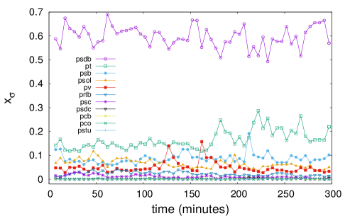
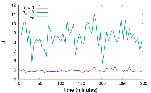
Refer to caption
Figure 1: Brazil General Elections 2014, q=11๐‘ž11q=11: time series of the user mean preferences, or normalized mean number of mentions, xฯƒโ€‹(t)subscript๐‘ฅ๐œŽ๐‘กx_{\sigma}(t). The acronyms stand for political parties names.
Refer to caption
Figure 2: Brazil General Elections 2014, q=11๐‘ž11q=11: coupling Jโ€‹(t)๐ฝ๐‘กJ(t) as solution of the inverse problem with (green) and without (purple) a uniform external field hqโ€‹(t)subscriptโ„Ž๐‘ž๐‘กh_{q}(t).
Refer to caption
Figure 3: Brazil General Elections 2014, q=11๐‘ž11q=11: macroscopic correlations from the data and from the MD and MFP models. An acronym in the horizontal axis indicates one of the q๐‘žq autocorrelations, while a pair of acronyms indicates one of the qโ€‹(qโˆ’1)/2๐‘ž๐‘ž12q(q-1)/2 connected correlation functions (for visual convenience, only a few are shown). For each model, Nโ€ฒsuperscript๐‘โ€ฒN^{\prime} represents the factor providing the effective number of messages Neโ€‹fโ€‹f=N/Nโ€ฒsubscript๐‘๐‘’๐‘“๐‘“๐‘superscript๐‘โ€ฒN_{eff}=N/N^{\prime} (see Sec. IVC)
Refer to caption
Figure 4: Brazil General Elections 2014 - Second Round, q=2๐‘ž2q=2: time series of the mean user preferences, or normalized mean number of mentions, xฯƒโ€‹(t)subscript๐‘ฅ๐œŽ๐‘กx_{\sigma}(t).
Refer to caption
Figure 5: Brazil General Elections 2014 - Second Round, q=2๐‘ž2q=2: macroscopic correlations (the first two on the left are autocorrelations). For each model, Nโ€ฒsuperscript๐‘โ€ฒN^{\prime} represents the factor providing the effective number of messages Neโ€‹fโ€‹f=N/Nโ€ฒsubscript๐‘๐‘’๐‘“๐‘“๐‘superscript๐‘โ€ฒN_{eff}=N/N^{\prime} (see Sec. IVC)
Refer to caption
Figure 6: Brazil General Elections 2014 - Second Round, q=2๐‘ž2q=2: coupling Jโ€‹(t)๐ฝ๐‘กJ(t) as solution of the inverse problem without external field.
Refer to caption
Figure 7: UK General Elections 2010, q=3๐‘ž3q=3: time series of the mean user preferences, or normalized mean number of mentions, xฯƒโ€‹(t)subscript๐‘ฅ๐œŽ๐‘กx_{\sigma}(t).
Refer to caption
Figure 8: UK General Elections 2010, q=3๐‘ž3q=3: coupling Jโ€‹(t)๐ฝ๐‘กJ(t) as solution of the inverse problem with (green) and without (purple) a uniform external field hqโ€‹(t)subscriptโ„Ž๐‘ž๐‘กh_{q}(t) (upper plot); residual error of the inverse problem, or cost function (bottom plot).
Refer to caption
Figure 9: UK General Elections 2010, q=3๐‘ž3q=3: macroscopic correlations from the data and from the MD and MFP models (the first three on the left are autocorrelations). For each model, Nโ€ฒsuperscript๐‘โ€ฒN^{\prime} represents the factor providing the effective number of messages Neโ€‹fโ€‹f=N/Nโ€ฒsubscript๐‘๐‘’๐‘“๐‘“๐‘superscript๐‘โ€ฒN_{eff}=N/N^{\prime} (see Sec. IVC)
Refer to caption
Figure 10: Spanish General Elections 2016, q=4๐‘ž4q=4: time series of the mean user preferences, or normalized mean number of mentions, xฯƒโ€‹(t)subscript๐‘ฅ๐œŽ๐‘กx_{\sigma}(t).
Refer to caption
Figure 11: Spanish General Elections 2016, q=4๐‘ž4q=4: coupling Jโ€‹(t)๐ฝ๐‘กJ(t) as solution of the inverse problem with (green) and without (purple) a uniform external field hqโ€‹(t)subscriptโ„Ž๐‘ž๐‘กh_{q}(t).
Refer to caption
Figure 12: Spanish General Elections 2016, q=4๐‘ž4q=4: residual error of the inverse problem, or cost function.
Refer to caption
Figure 13: Indian Election 2014, q=2+๐‘žlimit-from2q=2+sentiment: time series of two mean user preferences, or normalized mean number of mentions, x1โ€‹(t)subscript๐‘ฅ1๐‘กx_{1}(t) and x2โ€‹(t)subscript๐‘ฅ2๐‘กx_{2}(t), and a normalized sentiment seen as a further user x3โ€‹(t)subscript๐‘ฅ3๐‘กx_{3}(t).
Refer to caption
Figure 14: Indian Election, q=2+๐‘žlimit-from2q=2+ sentiment: coupling Jโ€‹(t)๐ฝ๐‘กJ(t) as solution of the inverse problem without external field.

5 Conclusions

Advanced Big Data technologies can allow to track efficiently the political orientations of a large number of Twitter users (order 105superscript10510^{5} or more) on the base of a massive number of Twitts (order 106superscript10610^{6} or more). Electoral events provide then an attractive benchmark to test the prediction power of such big polls. In the electoral events where a stationary condition applies, and the network of users can be considered as self organized, the system of Twitts can be mapped toward two simple models: MD and MFP. In both cases, the correlations decay as 1/Neโ€‹fโ€‹f1subscript๐‘๐‘’๐‘“๐‘“1/N_{eff}, Neโ€‹fโ€‹fsubscript๐‘๐‘’๐‘“๐‘“N_{eff} being a small fraction of the mean number of Twitts, and the discrimination between the two models can be easily done by looking at the formulas (23) and (56), respectively. However, only in the MD case polls can be reliable. In the MFP case, instead, the intrinsic symmetry among equally strong candidates, and the empirical observation that these systems lie close to their critical points, reveals that the winner in this kind of electoral events is rather the result of a large random fluctuation, preventing then the use of these Twitts for making predictions. The MD and MFP are the two simplest and somehow opposite effective models able to reproduce the observed statistics. The formal solution of the inverse problem shows that, richer models, which are generalized Potts models interpolating between the two, could in principle be used for getting better matchings and further insights. In such a desirable plan, however, the parameters involved in these models require the knowledge of the instantaneous activity of each Twitt, which constitute costly data (in fact, Twitter can release these data on customer demand). Furthermore, the solution of the corresponding inverse problem would require a massive analysis. At any rate, the empirical observation about the critical value of the coupling - a fact that we have observed in all the electoral events - deserves further investigations.

Acknowledgment

We thank Eiko Yoneki for letting us know the Ref. [6]. Work supported by PNPD/CAPES Grant N. 001/PPGFSC/2017.

References

References

  • [1] A. Tumasjan, T. O. Sprenger, P. G. Sandner, I. M. Welpe, โ€œPredicting Elections with Twitter: What 140 Characters Reveal about Political Sentimentโ€, Proceedings of the Fourth International AAAI Conference on Weblogs and Social Media, 178 (2010).
  • [2] Prabhsimran Singh, Ravinder Singh Sawhney, and Karanjeet Singh Kahlon, โ€œPredicting the Outcome of Spanish General Elections 2016 Using Twitter as a Toolโ€, in โ€œAdvanced Informatics for Computing Researchโ€, First International Conference, ICAICR, Jalandhar, India, (2017).
  • [3] A. Khatua, A. Khatua, K. Ghosh, N. Chaki, โ€œCan # Twitter_Trends Predict Election Results? Evidence from 2014 Indian General Electionโ€, 48th Hawaii International Conference on System Sciences (2015).
  • [4] N. Dwi Prasetyo and C. Hauff, โ€œTwitter-based Election Prediction in the Developing Worldโ€, HT โ€™15 Proceedings of the 26th ACM Conference on Hypertext & Social Media, 149 (2015).
  • [5] Murphy Choy, Michelle L.F. Cheong, Ma Nang Laik, Koo Ping Shung, โ€œA sentiment analysis of Singapore Presidential Election 2011 using Twitter data with census correctionโ€, arXiv:1108.5520 (2011).
  • [6] Antoine Boutet, Hyoungshick Kim, and Eiko Yoneki, โ€œWhatโ€™s in Twitter, I know what parties are popular and who you are supporting now!โ€, Soc. Netw. Anal. Min., DOI 10.1007/s13278-013-0120-1 (2013).
  • [7] http://g1.globo.com/politica/eleicoes/2014/apuracao-a-temperatura-no-twitter.html (2014).
  • [8] http://g1.globo.com/politica/eleicoes/2014/apuracao-2-turno-a-temperatura-no-twitter.html (2014).
  • [9] D. Gayo-Avello, โ€œA Balanced Survey on Election Prediction using Twitter Dataโ€, arXiv:1204.6441 (2012).
  • [10] Claudio Castellano, Santo Fortunato, and Vittorio Loreto, โ€œStatistical Physics of social dynamicsโ€, Rev. Mod. Phys. 81, 591 (2009).
  • [11] T. M. Liggett โ€œStochastic Interacting Systems: Contact, Voter and Exclusion Processesโ€ (New York: Springer), 1999.
  • [12] K. Sznajd-Weron, โ€œSznajd model and its applicationsโ€, Acta Physica Polonica B. 36(8), 2537 (2005).
  • [13] M. Nekovee, Y. Moreno, G. Bianconi, M. Marsili, โ€œTheory of rumour spreading in complex social networksโ€, Physica A 374 457 (2007).
  • [14] A. T. Bernardes, U. M. S. Costa, A. D. Araujo, D. Stauffer, โ€œDamage spreading, coarsening dynamics and distribution of political votes in Sznajd model on square latticeโ€, International Journal of Modern Physics C 12(2) 159 (2001).
  • [15] A. T, Bernardes, D. Stauffer, J. Kertรฉsz, โ€œElection results and the Sznajd model on Barabasi networkโ€, European Physical Journal B. 25 123 (2002).
  • [16] G. Travieso, L. F. Costa, โ€œSpread of opinions and proportional votingโ€, Phys. Rev. E 74 036112 (2006).
  • [17] S. Fortunato, C. Castellano, โ€œScaling and universality in proportional electionsโ€, Phy. Rev. Lett. 99 138701 (2007).
  • [18] A. Mondaini Calva~~a\tilde{\textrm{a}}o, N. Crokidakis, C. Anteneodo, โ€œStylized Facts in Brazilian Vote Distributionsโ€, PLoS ONE 10(9) e0137732 (2015).
  • [19] F. Y. Wu, Rev. Mod. Phys., 54, 235 (1982).
  • [20] R. Xiang, J. Neville, M. Rogati, โ€œModeling relationship strength in online social networksโ€, Proceedings of the 19th international conference on World wide web, 981 (2010).
  • [21] S. Aparicio, J. Villazoวน-Terrazas and G. ร€lvarez, โ€œA Model for Scale-Free Networks: Application to Twitterโ€, Entropy 17, 5848 (2015).
  • [22] M. Ostilli, E. Yoneki, I X. Y. Leung, Jose F. F. Mendes, P. Lio,ฬ€ J Crowcroft, S. Aparicio, J. Villazoวน-Terrazas and G. ร€lvarez, โ€œStatistical mechanics of rumour spreading in network communitiesโ€, Procedia Computer Science 1 2331 (2012).
  • [23] Juyong Park and M. E. J. Newman, โ€œStatistical mechanics of networksโ€, Phys. Rev. E 70, 066117 (2004).