Two-loop $N$-jettiness soft function for $pp\to 2j$ production

Abstract

We calculate the two-loop soft function for $pp\to jj$, $e^{+}e^{-}\to 4j$ or $ep\to 3j$ when the $N$-jettiness observable is measured. The result presented here makes up the necessary piece for realizing the full next-to-next-to-leading order predictions for these processes using the $N$-jettiness subtraction scheme.

I Introduction

The accumulation of the data set and the continuously increasing precision of the experimental analyses bring the physics program at the Large Hadron Collider (LHC) and other experiments the ability to search for new physics from the small deviations of the data from the Standard Model predictions. In order to fulfill such searches, the precision of the theoretical predictions from Quantum Chromodynamics (QCD) has to match the small experimental errors to reliably interpret the collider data. Currently, the only theoretical tool, with no known substitutes, enables us to make predictions for collider phenomenologies out of the first QCD principle is the perturbative calculation based on the systematic expansion of the strong coupling constant $\alpha_{s}$ or $\alpha_{s}L$ if large logarithmic correction $L$ is present. In recent years, tremendous efforts have been made in realizing the theoretical predictions for the physical processes at the colliders with a full control of the final state kinematics beyond the next-to-leading order (NLO) accuracy. On the fixed order side, significant progress has been made in the past few years, which includes achieving the fully differential gluon-gluon fusion Higgs ($H$) production Cieri:2018oms ; Dulat:2018bfe and the single jet production in deep-inelastic scattering Currie:2018fgr at next-to-next-to-next-to-leading order (N³LO) in $\alpha_{s}$ and the next-to-next-to-leading order (NNLO) calculations of the single inclusive jet or dijet productions Currie:2017eqf , $V/H+j$ processes Boughezal:2015dva ; Ridder:2015dxa ; Boughezal:2015ded ; Gehrmann-DeRidder:2017mvr ; Boughezal:2015dra ; Chen:2014gva ; Boughezal:2015aha , Higgs production through the vector boson fusion Cacciari:2015jma ; Cruz-Martinez:2018rod , single top Brucherseifer:2014ama ; Berger:2016oht and $t{\bar{t}}$ productions Czakon:2015owf ; Catani:2019iny at the LHC, the jet productions in deep-inelastic scattering Abelof:2016pby ; Currie:2017tpe , and the heavy flavor production in deep-inelastic neutrino scattering Berger:2016inr .

The rapid growth in the higher order predictions benefit from either the new higher loop calculations achieved or the theoretical schemes developed for dealing with the singularities in the real emissions. Recent achievements of the analytic two-loop five-point amplitude Abreu:2018aqd ; Chicherin:2018yne ; Chicherin:2018old highlight the current status of the loop calculations for the collider processes, and meanwhile new ideas are keeping on popping out Borowka:2018dsa ; Liu:2017jxz ; Liu:2018dmc ; Xu:2018eos . To handle the infrared (IR) singularities in the real corrections, various schemes have been proposed and successfully applied to the LHC phenomenology, such as the local subtraction schemes including the antenna subtraction GehrmannDeRidder:2005cm , the sector improved residue subtraction Czakon:2010td and the nested soft-collinear subtraction Caola:2017dug , as well as the physical observable based global schemes like the $q_{T}$-subtraction Catani:2007vq , inclusive jet mass subtraction Gao:2012ja and the $N$-jettiness subtraction Boughezal:2015dva ; Gaunt:2015pea . Although the global schemes are always criticized for the numerical instability, they have realized many interesting higher order predictions for the physical processes at the hadron colliders including the numerically most challenging Higgs production at N³LO Cieri:2018oms .

Among the local schemes, $N$-jettiness scheme is the known scheme being able to handle the IR singularities for generic jet processes at the hadron colliders. The scheme utilizes a threshold cut-off $\tau_{\rm cut}$ in the $N$-jettiness event shape $\tau$ Stewart:2010tn to distinguish between the NNLO $N$ jet (when $\tau<\tau_{\rm cut}$) and the NLO $N+1$ jet configurations ($\tau>\tau_{\rm cut}$). Below the $\tau_{\rm cut}$, a Soft-Collinear-Effective-Theory Bauer:2000ew ; Bauer:2000yr ; Bauer:2001ct ; Bauer:2001yt ; Bauer:2002nz approach based on the factorization theorem Stewart:2010tn

$$\mathrm{d}\sigma(\tau_{\rm cut})=B\,B\,{\rm Tr}[S\cdot H]\,\prod_{i=1}J_{i}+{\cal O}\left(\tau_{\rm cut}\right)\,,$$ (1)

is used to approximate the full QCD contribution. Here $B$ stands for the beam function due to the initial state energetic radiations while $J$’s are the jet functions for the final state collinear radiations. The hard function $H$ encodes the hard loop information. $S$ is the soft function for soft radiations. The trace is over the relevant color space. All the ingredients in the factorization theorem are universal except for the hard function $H$ which depends on the specific process under consideration. The difference between the factorization theorem and the full QCD is suppressed by power corrections in $\tau_{\rm cut}$, which have been studied extensively recently for the $0$-jettiness case Moult:2016fqy ; Boughezal:2016zws ; Moult:2017jsg ; Boughezal:2018mvf ; Ebert:2018lzn . The universal beam and the jet functions are all known analytically to two-loops Gaunt:2014xga ; Gaunt:2014cfa ; Becher:2006qw ; Becher:2010pd and recently some of them are even calculated at three-loop order Bruser:2018rad ; Banerjee:2018ozf ; Melnikov:2018jxb . As for the quark beam function, its NNLO longitudinal polarized counterpart is also known in the literature Boughezal:2017tdd . The calculation of the soft function is complicated by its explicit dependence on the full $N$-jettiness measure, therefore its analytic NNLO calculation is by far out of reach and people turn to numerical solutions. A generic framework was proposed in Boughezal:2015eha for calculating such soft functions with arbitrary numbers of jets and the $1$-jettiness soft functions in $pp$-collision were calculated using this scheme or similar approach for both the massless jet Boughezal:2015eha ; Campbell:2017hsw and the massive heavy flavor productions Li:2016tvb ; Li:2018tsq . However, at NNLO, the most general calculations can only be covered when one considers the $N$-jettiness soft function with four external hard legs, which is missing in the original calculations. In this manuscript, we present such calculation by extending the previously developed numerical method and show sufficient calculating details. We noticed a recent conference proceeding Bell:2018mkk on the $2$-jettiness soft function using pySecDec. Our work uses a different and independent approach which can serve as a cross check of the calculations.

The rest of this work is organized as follows. We discuss the numerical setups and the phase space parameterization in detail in Section II. In Section III, we present our numerical results for the $2$-jettiness observable in hardon-hadron collisions. Last we conclude in Section IV

II Computational Setup

In this section, we summarize the setups used in our calculation. We follow the general numerical framework proposed in Boughezal:2015eha , and show its capability in dealing with $N$-jettiness with four hard reference vectors in $pp\to jj$, $ep\to 3j$ and $0\to 4j$. We note that the calculations with four reference vectors go through all possible configurations in calculating any $N$-jettiness soft functions at NNLO. We clarify some of the computational details of this framework.

For simplicity, we stick to the hadronic $N$-jettiness definition which reads

$$\tau=\sum_{i}{\rm min}\left(n_{1}\cdot q_{i}\,,n_{2}\cdot q_{i}\,,\dots\,,n_{N}\cdot q_{i}\right)\,,$$ (2)

where $n_{i}$’s are the $N$ light-like hard reference vectors along the initial state hadronic beams or the final state jet axes and $q_{i}$’s are the four momentum of the soft radiations. We note that here all the hard vectors $n_{i}$’s are physical objects and are defined in $4$-dimension while the soft momentum $q_{i}$’s can potentially be un-resolvable and are therefore $d$-dimensional quantities, with $d=4-2\epsilon$ in the dimensional regularization. The soft function with $n$ real soft emissions then can be calculated by performing the phase space integration

$$S(\tau)=\prod^{n}_{i}\int\,\frac{\mathrm{d}^{d}q_{i}}{(2\pi)^{d-1}}\delta^{+}(q_{i}^{2})\,{\cal S}(\{q_{i}\})\,\Theta_{N,i}(\{q_{i}\})\,,$$ (3)

where we have introduced the $N$-jettiness measurement function

$$\Theta_{N,i}(\{q_{i}\})=\sum_{j=1}^{N}\delta(\tau-\sum_{i}^{n}n_{j_{i}}\cdot q_{i})\prod_{k_{i}\neq j_{i}}^{N-1}\theta(n_{k_{i}}\cdot q_{i}-n_{j_{i}}\cdot q_{i})\,,$$ (4)

and ${\cal S}$ is the soft current matrix element for the soft radiations which, up to NNLO, has been known for a long time Catani:1999ss ; Catani:2000pi . For $N$-jettiness with $3$ reference vectors , to NNLO, the soft current can be expressed in terms of a sum of dipole contributions, while starting from four reference vectors, like the case we study here, new triple-pole structure involving 3 eikonal lines arises which is induced by the one-loop soft current. The triple-pole contribution, which will be calculated later in this work, is the only remaining piece for calculating the $N$-jettiness soft function with arbitrary external eikonal lines at ${\cal O}(\alpha_{s}^{2})$. For completeness, we summarize the explicit form of the soft current ${\cal S}$ to ${\cal O}(\alpha_{s}^{2})$ in the Appendix V.1.

In order to compute the soft function numerically, the key step is to find a suitable momentum parameterization to allow us to write the phase space integration in the form of

$$\int_{0}^{1}\prod_{i}\mathrm{d}x_{i}\,x_{i}^{-1-a_{i}\epsilon}\,F(\{x_{i}\})=\int_{0}^{1}\prod_{i}\mathrm{d}x_{i}\,\left[-\frac{1}{a_{i}\,\epsilon}\delta(x_{i})+\left(\frac{1}{x_{i}}\right)_{+}+\dots\right]\,F(\{x_{i}\})\,,$$ (5)

which is ready for the Laurent expansion so as for us to identify all the $\epsilon$-poles and evaluate the coefficients of the poles numerically. We thus now turn to the discussion of the phase space parameterization for single and double real emissions with four reference directions, separately. We note that though we are focusing on the four reference vector case, the parameterization is general enough to be applicable directly to any $N$-jettiness computation at the NNLO. In all cases below, we utilize the Sudakov decomposition to write an arbitrary light-like four vector $k^{\mu}$ with respect to two of the reference vectors $n_{i}$ and $n_{j}$ as

$$k^{\mu}=\frac{n_{j}^{\mu}}{n_{ij}}k^{+}+\frac{n_{i}^{\mu}}{n_{ij}}k^{-}+k_{\perp}^{\mu}\,,\quad\quad{\rm\,denoted\,\,as}\quad k^{\mu}=(k^{+},k^{-},k_{\perp}^{i})\,,$$ (6)

with $k^{+}=n_{i}\cdot k$, $k^{-}=n_{j}\cdot k$ and $k_{\perp}\cdot n_{i}=k_{\perp}\cdot n_{j}=0$ and $|k_{\perp}|^{2}=\frac{2}{n_{ij}}k^{+}k^{-}$. Here we have introduced the notation $n_{ij}\equiv n_{i}\cdot n_{j}$.

II.1 single real emission phase space parameterization

With 4 reference vectors, $n_{i}$, $n_{j}$, $n_{k}$ and $n_{l}$, at hand, for one real emission with momentum $q_{1}^{\mu}$ for computing the NLO soft function or the NNLO real-virtual contribution, we can parameterize all the involved vectors with respect to $n_{i}$ and $n_{j}$, which are

$$n^{\mu}_{k}=(n_{k}^{+},n_{k}^{-},0,n_{k}^{\perp}\,;0)\,,$$

$$n^{\mu}_{l}=(n_{l}^{+},n_{l}^{-},n_{l}^{\perp}s_{\phi_{l}},n^{\perp}_{l}\,c_{\phi_{l}}\,;0)\,,$$

$$q_{1}^{\mu}=(q_{1}^{+},q_{1}^{-},q_{1}^{\perp}s_{\phi_{1}}c_{\alpha_{1}},q_{1}^{\perp}\,c_{\phi_{1}}\,;q_{1}^{\perp}s_{\phi_{1}}s_{\alpha_{1}}\,,0)\,,$$ (7)

where we have used the freedom to choose the azimuthal angle of the vector $n_{k}$ and the additional $\epsilon$-angles other than $\alpha_{1}$ to be $0$. Here $\alpha_{1}\,,\phi_{l}\,,\phi_{1}\in[0,\pi]$ with

$$c_{\phi_{l}}=\frac{n_{ik}n_{jl}+n_{il}n_{jk}-n_{ij}n_{kl}}{2\sqrt{n_{ik}n_{il}n_{jk}n_{jl}}}\,.$$ (8)

Here the non-zero $\phi_{l}$ makes $n_{k}$ and $n_{l}$ span the azimuthal plain and therefore $\alpha_{1}$ is necessary for parameterizing the $d$-dimensional momentum $q_{1}$, since $q_{1}$ in general lies outside the pain $n_{k}$ and $n_{l}$ belong to. We note that since the reference vectors $n_{i}$’s are physical, for arbitrary numbers of the reference vectors, their “$\perp$”-components will all be lying in one azimuthal plain, and thus Eq. (II.1) is the most general parameterization for computing the $N$-jettiness function with arbitrary $N$. For the processes similar to what we are considering here, the transverse components $n_{k}^{\perp}$ and $n_{l}^{\perp}$ have to align with each other ($\phi_{l}=0$ or $\pi$) due to the momentum conservation, therefore one can simplify the parameterization by setting $\alpha_{1}=0$ which reduces to the parameterization used in Boughezal:2015eha ; Campbell:2017hsw for computing $1$-jettiness.

Although in general $n_{i}$ and $n_{j}$ can be chosen arbitrarily for performing the Sudakov decomposition, in order to correctly isolate the $\epsilon$-poles, it is more useful to choose $n_{i}$ so that $n_{i}\cdot q$ contributes to $\tau$ as set by $\Theta_{N,i}$ while $n_{j}\cdot q$ appears as one of the singular poles in the denominator of the soft current matrix ${\cal S}$. With this parameterization, for non-zero $\alpha$, the phase space integration for single emission can be modified to

$$\int\frac{\mathrm{d}^{d}q_{1}}{(2\pi)^{d-1}}\,\delta^{+}(q_{1}^{2})F(q_{1})\delta(\tau-n_{i}\cdot q_{1})\theta(n_{j}\cdot q_{1}-n_{i}\cdot q_{1}) = \frac{\pi}{4}\,\left(\frac{2}{n_{ij}}\right)^{1-\epsilon}\,\left(\frac{1}{2\pi}\right)^{3-2\epsilon}\,\tau^{-1-2\epsilon}\,$$ (9)

$$\times\frac{2\pi^{-\epsilon}}{\Gamma(1-\epsilon)}\,\frac{1}{2}\int_{0}^{1}\,\mathrm{d}x_{1}\,\mathrm{d}x_{2}\,\mathrm{d}x_{3}\,x_{1}^{-1+\epsilon}\,\frac{-\epsilon}{x_{3}^{1+\epsilon}}\,\,\left[2^{2}s_{\phi_{1}}^{2}(1-x_{3})\right]^{-\epsilon}\,\left[\tau^{2}x_{1}^{-1}\right]\,\Big{[}F(x_{3})+F(1-x_{3})\Big{]}\,,$$

where we have made the variable changes

$$q_{1}^{-}=\frac{\tau}{x_{1}}\,,\quad c_{\phi_{1}}=\pi\,x_{2}\,,\quad c_{\alpha_{1}}=1-2x_{3}\,.$$ (10)

It can also be shown that for $\alpha_{1}=0$, one can further modify the phase space integration to make $\phi_{1}\in[0,2\pi]$ when taking into account the properties of the soft current and the $N$-jettiness observable, as has been done in Boughezal:2015eha .

Eq. (9) is our starting point for calculating the single emission contributions to the soft function numerically and we list in the Appendix V.2 all the final forms of the phase space integrations suitable for direct numerical evaluation of the one emission contributions.

II.2 double real emission phase space parameterization

Now we sketch the parameterization for the double real emission with momenta $q_{1}$ and $q_{2}$ at NNLO. We want to add on top of Eq. (II.1) the momentum $q_{2}$ parameterization, meanwhile require that the dot product $q_{1}^{\perp}\cdot q_{2}^{\perp}$ only relies on the azimuthal angle between these two vectors, so as to use the non-linear transformation Boughezal:2015eha in a later stage for the purpose of pole isolation. To find the particular parameterization of $q_{2}$, we first rotate Eq. (II.1) around the $n_{k^{\perp}}$ axis by $\alpha_{1}$ to eliminate the $\alpha_{1}$ dependence in $q_{1}^{\mu}$, then we rotate in the azimuthal plain by $\phi_{1}$ to align the $x$-axis with $q_{1}^{\perp}$ to further remove the dependence of $\phi_{1}$ in the parameterization of $q_{1}^{\mu}$. These rotational operations lead to the momentum representation

$$q_{1}^{\mu}=(q_{1}^{+}\,,q_{1}^{-}\,,0\,,q_{1}^{\perp};0)\,,$$

$$n_{k}^{\mu}=(n_{k}^{+}\,,n_{k}^{-}\,,-n_{k}^{\perp}s_{\phi_{1}}\,,n_{k}^{\perp}c_{\phi_{1}};0)\,,$$

$$n_{l}^{\mu}=(n_{l}^{+}\,,n_{l}^{-}\,,n_{l}^{\perp}s^{\alpha_{1}}_{\phi_{l}-\phi_{1}}\,,n_{l}^{\perp}\,c_{\phi_{l}-\phi_{1}}^{\alpha_{1}};-n_{l}^{\perp}s_{\phi_{l}}\,s_{\alpha_{1}},0)\,,$$ (11)

where we introduced the notation $c^{\alpha_{1}}_{\phi_{l}-\phi_{1}}\equiv c_{\phi_{l}}c_{\phi_{1}}+s_{\phi_{l}}s_{\phi_{1}}c_{\alpha_{1}}$. It is now straightforward to see that to satisfy our requirements, $q_{2}^{\mu}$ can be parameterized (in this frame after rotation) as

$$q_{2}^{\mu}=(q_{2}^{+}\,,q_{2}^{-}\,,q_{2}^{\perp}s_{\phi_{2}}c_{\alpha_{2}}\,,q_{2}^{\perp}c_{\phi_{2}};q_{2}^{\perp}s_{\phi_{2}}s_{\alpha_{2}}c_{\beta}\,,q_{2}^{\perp}s_{\phi_{2}}s_{\alpha_{2}}s_{\beta},0)\,,$$ (12)

so that $q^{\perp}_{1}\cdot q^{\perp}_{2}=-|q^{\perp}_{1}||q_{2}^{\perp}|\,c_{\phi_{2}}$. The $\beta$ angle here is necessary to guarantee that the $\epsilon$-components of $q_{1}$ and $q_{2}$ are not always aligned with each other. Due to the Lorenz invariance of the individual emission phase space measure, the rotational operations used to derive the parameterization of $q_{2}$ do not introduce any complexity to the Jacobian of the phase space integration. We also note that the parameterization derived here is the most general for computing the double real contributions to any $N$-jettiness soft functions. As for the processes we are interested in in this work, using the same momentum conservation for the single real emission case, one can set $\alpha_{1}$ and $\beta$ to $0$ to simplify the phase space integration.

Within this parameterization, the dot product $q_{1}\cdot q_{2}$ takes the form

$$q_{1}\cdot q_{2}=\frac{1}{n_{ij}}\left[q_{1}^{+}q_{2}^{-}+q_{1}^{-}q_{2}^{+}-2\sqrt{q_{1}^{+}q_{2}^{-}q_{1}^{-}q_{2}^{+}}c_{\phi_{2}}\right]\,,$$ (13)

which generates a linear singularity in the double real soft current if $q_{1}$ be collinear to $q_{2}$ is possible, which prevents us from extracting the $\epsilon$-poles using the Laurent expansion in Eq. (5). To extract the poles, the angle $c_{\phi_{2}}$ is further parameterized as $c_{\phi_{2}}=1-2\eta$, with the non-linear parameterization

$$\eta=\frac{\left(\sqrt{q_{1}^{+}q_{2}^{-}}-\sqrt{q_{1}^{-}q_{2}^{+}}\right)^{2}(1-x^{\prime})}{\left(\sqrt{q_{1}^{+}q_{2}^{-}}-\sqrt{q_{1}^{-}q_{2}^{+}}\right)^{2}+4\sqrt{q_{1}^{+}q_{2}^{-}q_{1}^{-}q_{2}^{+}}x^{\prime}}\,,\quad\quad x^{\prime}=\sin^{2}\left(\frac{\pi}{2}x\right)\,,$$ (14)

if the soft momentum $q_{1}$ and $q_{2}$ can be collinear to each other, and

$$\eta=x^{\prime}\,,\quad\quad x^{\prime}=\sin^{2}\left(\frac{\pi}{2}x\right)\,,$$ (15)

if $q_{1}$ and $q_{2}$ can no way be collinear as constrained by the jettiness measurement, for instance when $\tau=n_{i}\cdot q_{1}+n_{j}\cdot q_{2}$.

Last we comment on the choice of $n_{i}$ and $n_{j}$ in the Sudakov decomposition. The same logic follows the single emission case. The reference vectors $n_{i}$ and $n_{j}$ are chosen if $n_{i}\cdot q_{1}$ and $n_{j}\cdot q_{2}$ contribute to $\tau$, i.e. $\tau=n_{i}\cdot q_{1}+n_{j}\cdot q_{2}$. Otherwise, if both $n_{i}\cdot q_{1}$ and $n_{i}\cdot q_{2}$ contribute to the jettiness observable, then $n_{i}$ will be naturally picked as one reference axis for the decomposition, and for convenience, $n_{j}$ is chosen in the way that the double real soft current is singular as $n_{j}\cdot q_{1}\to 0$ and/or $n_{j}\cdot q_{2}\to 0$. Additional variable changes are needed to map all variables onto the regime $[0,1]$ suitable for doing the Laurent expansion. The mapping is standard in the sector decomposition calculations and has been detailed in Campbell:2017hsw ; Li:2018tsq . After the mapping, in the cases where one encounters the fractional power of the form $s^{-\frac{1}{2}+\epsilon}$ with $s\in[0,1]$, a further variable transform $s=\sin^{2}\left(\frac{\pi}{2}x\right)$, with $x\in[0,1]$, is then used.

III Numerical Results

In this section, we present our main results. We highlight our results using the $2$-jettiness soft function to ${\cal O}(\alpha_{s}^{2})$ in $pp\to jj$. Other processes such as $e^{+}e^{-}\to 4j$ can be easily obtained by changing properly the values of $\lambda_{ij}$ in Eq. (21), without doing any additional integrations. The $2$-jettiness soft function depends on four hard directions, which we denote as $n_{1}$, $n_{2}$, $n_{3}$ and $n_{4}$. We align $n_{1}$ and $n_{2}$ with the incoming beam axes in the $\pm z$-directions, and let $n_{3}$ and $n_{4}$ lie along the outgoing jet directions. For the purpose of presenting, though not at all required in our calculation, we let the incoming partons carry exactly the same energy in the collision and show the $2$-jettiness soft function as a function of $n_{13}$ and we present the results in the Laplacian space $\int_{0}^{\infty}\mathrm{d}\tau\,e^{-\tau\,z}\sigma(\tau)$.

We start from the NLO soft function. At NLO, the renormalized $2$-jettiness soft function can be written as a sum of dipole terms

$$S^{(1)}=\frac{\alpha_{s}}{4\pi}\sum_{i\neq j}T_{i}\cdot T_{j}\left(4C^{(1,-1)}_{ij}\tilde{L}^{2}\,+4C^{(1,0)}_{ij}\tilde{L}\,+\left[2C^{(1,1)}_{ij}+\frac{2}{3}\pi^{2}C^{(1,-1)}_{ij}\right]\right)\equiv\sum_{i\neq j}T_{i}\cdot T_{j}S_{ij}^{(1)}\,,\quad$$ (16)

where $C_{ij}^{(1,i)}$ are the coefficients of the $\epsilon^{i}$-poles returned by our calculation using the method for single emission as sketched before. The coefficients of the logarithmic terms $\tilde{L}^{2}$ and $\tilde{L}$ can be predicted by solving the renormalization group equation (RGE) of the soft function and therefore serve as checks of our numerical approach.

In fig. 1, we show the NLO coefficients of the $\tilde{L}^{n}$ ($n=2,1,0$) terms for dipole $S_{12}^{(1)}$ and $S_{13}^{(1)}$ as functions of $n_{13}$. These are the only independent terms in the special kinematics we have chosen.

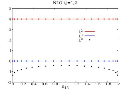
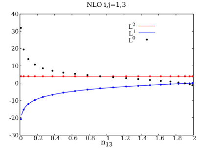
Figure 1: Coefficients of the $\tilde{L}^{n}$ terms for the ${\cal O}(\alpha_{s})$ $2$-jettiness soft function in $pp\to jj$ production, normalized to $\frac{\alpha_{s}}{4\pi}T_{i}\cdot T_{j}$.

In both cases, we have normalized the results to $\frac{\alpha_{s}}{4\pi}$. The red, blue and black dots represent the coefficients for $\tilde{L}^{2}$, $\tilde{L}^{1}$ and $\tilde{L}^{0}$ from our numerical set-ups, respectively. The solid lines are obtained by solving the RGE analytically. We see perfect agreements between the analytic results and our numerical predictions, which implies the validity of the computational framework at this order.

At NNLO, other than the abelian terms which can be obtained by exponentiate the NLO results, the soft function receives non-abelian contributions from the $q{\bar{q}}$-emission, the $gg$-emission, the real-virtual corrections and the renormalization. The real-virtual corrections can be further broke down to the dipole and the triple-pole contributions, and the rest are of the dipole forms. The summation of all the dipole contributions can be organized by the color factors $C_{A}$ and $N_{F}T_{R}$, while the triple-pole real-virtual corrections can be massaged into one single color term $f_{abc}T^{a}_{1}T^{b}_{2}T^{c}_{3}$ with the help of the color charge conservation $\sum T_{i}=0$. The final results of the NNLO soft function can therefore be written as

$$S^{(2)} = \frac{1}{4}\sum_{i\neq j,k\neq l}\{T_{i}\cdot T_{j},T_{k}\cdot T_{l}\}\,S^{(1)}_{ij}S^{(1)}_{kl}$$ (17)

$$+\left(\frac{\alpha_{s}}{4\pi}\right)^{2}\,\left(\sum_{i\neq j}T_{i}\cdot T_{j}\left[C_{A}S_{ij}^{(2),C_{A}}+N_{F}T_{R}S_{ij}^{(2),N_{F}}\right]+f_{abc}T_{1}^{a}T_{2}^{b}T_{3}^{c}\,S_{123}^{(2)}\right)\,,$$

where all the NNLO dipoles $S_{ij}^{(2)}$ and triple-pole $S_{123}^{(2)}$ in the non-abelian terms can be written as a series in terms of the logarithms $\tilde{L}$. And once again, all the coefficients of those logarithmic terms $\tilde{L}^{n}$ with $n=3,2,1$ can be predicted by RGE with the knowledge of the full NLO results obtained before.

The coefficients of the $N_{F}T_{R}$ terms for the dipoles $S_{12}^{(2)}$ and $S_{13}^{(2)}$ are shown in fig. 2, which include the contributions from the $q{\bar{q}}$ emission and the $N_{F}$ term in the renormalization.

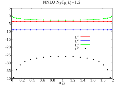
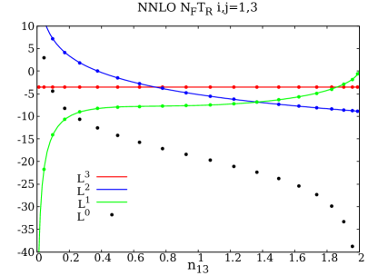
Figure 2: Coefficients of the $\tilde{L}^{n}$ with $n=3,2,1,0$ in $S_{12}^{(2),N_{F}}$ (left panel) and $S_{13}^{(2),N_{F}}$ (right panel).

.

Perfect agreements are observed between the numerical calculations of the $\tilde{L}^{n}$ coefficients for $n=3,2,1$ as shown in colored dots and the RGE predictions in solid lines, which validates not only the NNLO computations of the $N_{F}$ contributions but also the correctness of the non-logarithmic term in the NLO calculations. The NNLO non-logarithmic prediction (in black dots) displayed here is not presented in the original NNLO $N$-jettiness soft paper Boughezal:2015eha and is one of our main results of this work. We note that the NNLO results here and below are also presented in a conference proceeding Bell:2018mkk in a different way with a different approach.

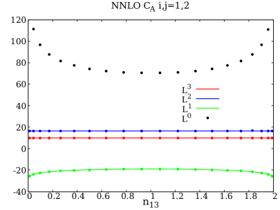
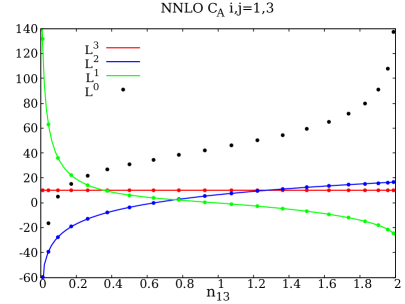
Figure 3: Coefficients of the $\tilde{L}^{n}$ with $n=3,2,1,0$ in $S_{12}^{(2),C_{A}}$ (left panel) and $S_{13}^{(2),C_{A}}$ (right panel).

.

Same situation happens to the $C_{A}$ term, as displayed in fig. 3, in which we also compared $\tilde{L}^{n}$ coefficients from the numerical calculation against the results from the RGE to find no difference. The non-logarithmic coefficients are represented by the black dots.

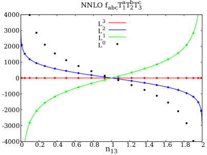
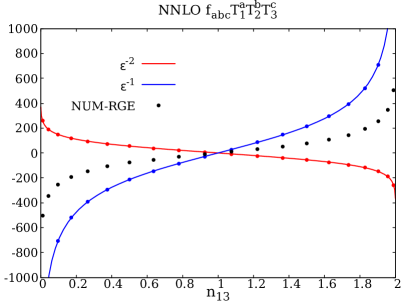
Figure 4: Coefficients of the $\tilde{L}^{n}$ with $n=3,2,1,0$ in $S_{123}^{(2)}$ (left panel) and the $\epsilon$-pole terms (right panel).

.

Last we give the prediction for the triple-pole term $S_{123}^{(2)}$, which arises firstly for four hard reference directions. Just like the dipole contributions, the logarithms in the triple-pole are still predictable from the RGE. The analytic predictions are once again found to agree with our numerical results, as clearly seen in the left panel of fig. 4. Other than that, we also compare the $\epsilon$-pole terms without the $\tilde{L}$’s from our numerical calculations with the ones predicted by the RGEs and find satisfactory agreements. The result for the non-logarithmic term (left panel in fig. 4) as well as the term entirely unpredictable from RGE (right panel, normalized further to $-2\pi$) are indicated in black dots, which finalizes all the NNLO contributions to the $2$-jettiness for the $pp\to jj$ process.

IV Conclusions

In this work, we present the calculation of the $N$-jettiness soft function with four hard reference directions using the computational framework proposed in Boughezal:2015eha using the approach of sector decomposition. We generalize the parameterizations used for the $1$-jettiness calculation to the arbitrary $N$-jettiness case. We specifically calculated the NNLO $N$-jettiness soft function with four external hard legs, where the last new piece at this order, the triple-pole configuration, first arises. We managed to isolate all the singularities from the soft function integrands and reduce the computation to a set of numerical integrals which are ready to evaluate. We check the numerically computed logarithmic terms in the soft function against the predictions from the RGEs and found perfect agreements. The non-logarithmic terms which can not be obtained through the known RGEs are calculated directly in this work. We expect the result obtained in this manuscript to find its quick applications in both the fixed NNLO calculations and achieving the parton shower matching Alioli:2013hqa for the relevant processes.

V Acknowledgments

This work is supported by the National Natural Science Foundation of China under Grant No. 11775023 and the Fundamental Research Funds for the Central Universities. S.J. is supported by the BNU JingShi Undergraduate Fellowship.

Appendix

V.1 soft current

For completeness, we list all the soft current matrix elements here, which were first derived in the seminal works Catani:1999ss and Catani:2000pi by Catani and Grazzini.

The NLO soft current with one soft emission $q$ is given by

$${\cal S}^{(1)}=-(4\pi\alpha_{s}\mu^{2\epsilon})\times 2\times\sum_{i\neq j}T_{i}\cdot T_{j}\,{\cal S}^{(1)}_{ij}(q)\,,$$ (18)

with the NLO dipole given by

$${\cal S}^{(1)}_{ij}(q)=\frac{n_{ij}}{2\,n_{i}\cdot q\,n_{j}\cdot q}\,.$$ (19)

The NNLO real-virtual correction can be written as the sum of the dipole ${\cal S}^{(2)}_{RV,dipole}$ and triple-pole ${\cal S}^{(2)}_{RV,tri.}$ contributions, with the dipole contribution be

$${\cal S}^{(2)}_{RV,dipole}=\frac{(4\pi\alpha_{s}\,\mu^{2\epsilon})^{2}}{4\pi^{2}}\,\times\frac{(4\pi)^{\epsilon}}{\epsilon^{2}}\,\frac{\Gamma^{4}(1-\epsilon)\,\Gamma^{3}(1+\epsilon)}{\Gamma^{2}(1-2\epsilon)\,\Gamma(1+2\epsilon)}\,\times\,C_{A}\,\,\sum_{i\neq j}T_{i}\cdot T_{j}\,\left[{\cal S}^{(1)}_{ij}(q)\right]^{1+\epsilon}\,,$$ (20)

and the triple-pole term

$${\cal S}^{(2)}_{RV,tri.} = \frac{(4\pi\alpha_{s}\mu^{2\epsilon})^{2}}{4\pi^{2}}\times\frac{(4\pi)^{\epsilon}}{\epsilon^{2}}\,\frac{\Gamma^{3}(1-\epsilon)\Gamma^{2}(1+\epsilon)}{\Gamma(1-2\epsilon)}\,2\sin(\pi\epsilon)$$ (21)

$$\times\sum_{i\neq j\neq k}\,f_{abc}T_{k}^{a}\,T_{i}^{b}\,T_{j}^{c}\,\,\left(\lambda_{ij}-\lambda_{iq}-\lambda_{jq}\right)\,\,{\cal S}_{ki}(q)\left[{\cal S}_{ij}(q)\right]^{\epsilon}\,\,,$$

where $\lambda_{ij}=1$ if $i$ and $j$ are both incoming or outgoing, otherwise $\lambda_{ij}=0$.

The NNLO real-real emission is given by

$${\cal S}_{q{\bar{q}}}^{(2)}=-\frac{1}{2}(4\pi\alpha_{s}\mu^{2\epsilon})^{2}\,T_{R}N_{F}\sum_{i\neq j}T_{i}\cdot T_{j}\,{\cal J}_{ij}\,,$$ (22)

from the $q{\bar{q}}$ emission. To get this form we have used the color charge conservation $\sum_{i}T_{i}=0$. Here

$${\cal J}_{ij}={\cal I}_{ii}+{\cal I}_{jj}-2{\cal I}_{ij}\,,$$ (23)

and

$${\cal I}_{ij}=-\frac{2n_{ij}\,q_{1}\cdot q_{2}+\,n_{i}\cdot(q_{1}-q_{2})\,n_{j}\cdot(q_{1}-q_{2})}{2(q_{1}\cdot q_{2})^{2}\,\,n_{i}\cdot(q_{1}+q_{2})n_{j}\cdot(q_{1}+q_{2})}\,,$$ (24)

where $q_{1}$ and $q_{2}$ are the momentum carried by the real emissions. We denote the term proportional to $2\,n_{ij}\,q_{1}\cdot q_{2}$ as ${\cal I}_{ij}^{\rm II}$ and the rest ${\cal I}_{ij}^{\rm I}$.

And the $gg$ emission gives the non-abelian contribution

$${\cal S}_{gg,non-abe.}^{(2)}=-\frac{1}{2}\,\left(4\pi\alpha_{s}\mu^{2\epsilon}\right)^{2}\,C_{A}\,\sum_{i\neq j}\,T_{i}\cdot T_{j}\,{\cal T}_{ij}\,,$$ (25)

with

$${\cal T}_{ij}=2{\cal S}_{ij}-{\cal S}_{ii}-{\cal S}_{jj}\,,$$ (26)

where

$${\cal S}_{ij}={\cal S}_{ij}^{\rm s.o.}-\frac{1}{2}\,\frac{n_{i}\cdot q_{1}\,n_{j}\cdot q_{2}+n_{i}\cdot q_{2}\,n_{j}\cdot q_{1}}{n_{i}\cdot(q_{1}+q_{2})\,n_{j}\cdot(q_{1}+q_{2})}\,{\cal S}_{ij}^{\rm s.o.}+(1-\epsilon)\,{\cal I}_{ij}^{\rm I}+2\,{\cal I}_{ij}^{\rm II}\,,$$ (27)

and the current in the strongly ordering limit

$${\cal S}_{ij}^{\rm s.o.} = \frac{n_{ij}}{q_{1}\cdot q_{2}}\,\left(\frac{1}{n_{i}\cdot q_{1}\,n_{j}\cdot q_{2}}+\frac{1}{n_{j}\cdot q_{1}\,n_{i}\cdot q_{2}}\right)-\frac{n_{ij}^{2}}{n_{i}\cdot q_{1}\,n_{i}\cdot q_{2}\,n_{j}\cdot q_{1}\,n_{j}\cdot q_{2}}\,.$$ (28)

The abelian piece for the $gg$ double real emission is

$${\cal S}_{gg,abelian}^{(2)}=4\times(4\pi\alpha_{s}\mu^{2\epsilon})^{2}\times\frac{1}{2}\sum_{i\neq j,k\neq l}\{T_{i}\cdot T_{j}\,,T_{k}\cdot T_{l}\}{\cal S}_{ij}^{(1)}(q_{1})\,{\cal S}_{kl}^{(1)}(q_{2})\,.$$ (29)

V.2 numerical integrations for single emission

Here we list all final numerical integrations for evaluate single emission contributions. We note again that though we only show the $N$-jettiness with four hard directions $n_{i}$, $n_{j}$, $n_{k}$ and $n_{l}$, the parameterization here presented here is general enough for any $N$-jettiness soft functions. To extend to the case with more reference vectors, one simply insert more $\theta$ functions originated from the $N$-jettiness measurements. We use the notation $q||n_{i}$ to denote the separation of $q$ and $n_{i}$ is the smallest and thus $\tau=n_{i}\cdot q$.

V.2.1 final forms for numerical integration at NLO

At NLO, the contribution can be written as a sum of dipoles. We assume that the soft momentum $q$ is emitted from dipole $ij$. For the integrations shown below, we have extracted out an overall factor $-16\pi^{2}\left(\frac{\alpha_{s}}{2\pi}\right)\left(\frac{e^{\gamma_{E}}}{4\pi}\right)^{\epsilon}T_{i}\cdot T_{j}$.

• case 1: $q_{1}\parallel n_{i}$.

  For $q_{1}\parallel n_{i}$, the final form suitable for numerical integration is

  $$I^{i,{(1)}}_{ij} = \frac{\pi}{4}\left(\frac{n_{ij}}{2}\right)^{\epsilon}\left(\frac{1}{2\pi}\right)^{3-2\epsilon}\tau^{-1-2\epsilon}\frac{2\pi^{-\epsilon}}{\Gamma(1-\epsilon)}\frac{1}{2}\int_{0}^{1}\mathrm{d}x_{1}\mathrm{d}x_{2}\mathrm{d}x_{3}\,x_{1}^{-1+\epsilon}\frac{-\epsilon}{x_{3}^{1+\epsilon}}\left[2^{2}s_{\phi_{1}}^{2}(1-x_{3})\right]^{-\epsilon}$$ (30)

  $$\times\Big{[}F^{ij}_{i}(x_{3})+F^{ij}_{i}(1-x_{3})\Big{]}\,,$$

  where we have defined

  $$F^{ij}_{i}(x_{3})=\theta\big{(}A_{ij,k}(x_{1},c_{\phi_{1}})-x_{1}\big{)}\theta\big{(}A_{ij,l}(x_{1},c^{\alpha_{1}}_{\phi_{l}-\phi_{1}})-x_{1}\big{)}\,,$$ (31)

  and

  $$A_{ij,k}(x,c_{\phi})=\frac{n_{ik}}{n_{ij}}+\frac{n_{jk}}{n_{ij}}x-\sqrt{\frac{2x}{n_{ij}}}n_{k}^{\perp}c_{\phi}\,.$$ (32)

  As for the case in which $q_{1}\parallel n_{j}$, the result can be obtained by switching $i$ and $j$ in Eq. (30).

• case 2: $q_{1}\parallel n_{k}$.

  While for $q_{1}\parallel n_{k}$, we choose $n_{k}$ and $n_{i}$ to be the reference vectors, to have $q_{1}^{+}=n_{k}\cdot q_{1},q_{1}^{-}=n_{i}\cdot q_{1}$. Following the same variable changes shown in Eq. (10), we get the final form for the numerical evaluation

  $$I^{k,{(1)}}_{ij} = \frac{\pi}{4}\frac{n_{ij}}{n_{ik}}\left(\frac{n_{ik}}{2}\right)^{\epsilon}\left(\frac{1}{2\pi}\right)^{3-2\epsilon}\tau^{-1-2\epsilon}\frac{2\pi^{-\epsilon}}{\Gamma(1-\epsilon)}\frac{1}{2}\int_{0}^{1}\mathrm{d}x_{1}\mathrm{d}x_{2}\mathrm{d}x_{3}\,x_{1}^{\epsilon}\frac{-\epsilon}{x_{3}^{1+\epsilon}}\frac{\left[2^{2}s_{\phi_{1}}^{2}(1-x_{3})\right]^{-\epsilon}}{A_{ki,j}(x_{1},c_{\phi_{1}})}$$ (33)

  $$\times\Big{[}F^{ij}_{k}(x_{3})+F^{ij}_{k}(1-x_{3})\Big{]}\,,$$

  where

  $$F^{ij}_{k}(x_{3})=\theta\big{(}A_{ki,j}(x_{1},c_{\phi_{1}})-x_{1}\big{)}\theta\big{(}A_{ki,l}(x_{1},c^{\alpha_{1}}_{\phi_{l}-\phi_{1}})-x_{1}\big{)}\,.$$ (34)

  Again, we can switch $k$ and $l$ to obtain the $q_{1}\parallel n_{l}$ contribution.

V.2.2 final forms for $2$-parton correlated real-virtual contribution

For the $2$-parton correlated real-virtual contribution, we have for our numerical evaluation

• case 1: $q_{1}\parallel n_{i}$.

  $$I^{i,{(2)}}_{ij,{\rm RV}} = \frac{\pi}{4}\left(\frac{n_{ij}}{2}\right)^{2\epsilon}\left(\frac{1}{2\pi}\right)^{3-2\epsilon}\tau^{-1-4\epsilon}\frac{2\pi^{-\epsilon}}{\Gamma(1-\epsilon)}\frac{1}{2}\int_{0}^{1}\mathrm{d}x_{1}\mathrm{d}x_{2}\mathrm{d}x_{3}\,x_{1}^{-1+2\epsilon}\frac{-\epsilon}{x_{3}^{1+\epsilon}}\left[2^{2}s_{\phi_{1}}^{2}(1-x_{3})\right]^{-\epsilon}$$ (35)

  $$\times\Big{[}F^{ij}_{i}(x_{3})+F^{ij}_{i}(1-x_{3})\Big{]}\,,$$

• case 2: $q_{1}\parallel n_{k}$.

  $$I^{k,{(2)}}_{ij,{\rm RV}} = \frac{\pi}{4}\frac{n_{ij}}{n_{ik}}\left(\frac{n_{ij}n_{ik}}{4}\right)^{\epsilon}\left(\frac{1}{2\pi}\right)^{3-2\epsilon}\tau^{-1-4\epsilon}\frac{2\pi^{-\epsilon}}{\Gamma(1-\epsilon)}\frac{1}{2}\int_{0}^{1}\mathrm{d}x_{1}\mathrm{d}x_{2}\mathrm{d}x_{3}\,x_{1}^{3\epsilon}\frac{-\epsilon}{x_{3}^{1+\epsilon}}\frac{\left[2^{2}s_{\phi_{1}}^{2}(1-x_{3})\right]^{-\epsilon}}{\Big{[}A_{ki,j}(x_{1},c_{\phi_{1}})\Big{]}^{1+\epsilon}}$$ (36)

  $$\times\Big{[}F^{ij}_{k}(x_{3})+F^{ij}_{k}(1-x_{3})\Big{]}\,.$$

Here we have normalized to

$$16\pi^{2}\left(\frac{\alpha_{s}}{2\pi}\right)^{2}\left(\frac{e^{\gamma_{E}}}{4\pi}\right)^{2\epsilon}\frac{(4\pi)^{\epsilon}}{\epsilon^{2}}\frac{\Gamma^{4}(1-\epsilon)\Gamma^{3}(1+\epsilon)}{\Gamma^{2}(1-2\epsilon)\Gamma(1+2\epsilon)}C_{A}T_{i}\cdot T_{j}\,.$$ (37)

The $q||n_{j}$ and $q||n_{l}$ cases can be easily obtained by switching properly the indices.

V.2.3 final forms for 3-parton correlated real-virtual contribution

Now we turn to the triple-pole case in the real-virtual correction, in which $3$-parton correlated emission contributes. This configuration first arises in this case with four external legs. We assume the soft emission is from triple-pole $ijk$. And we normalize our results to

$$32\pi^{2}\left(\frac{\alpha_{s}}{2\pi}\right)^{2}\left(\frac{e^{\gamma_{E}}}{4\pi}\right)^{2\epsilon}\frac{(4\pi)^{\epsilon}}{\epsilon^{2}}\frac{\Gamma^{3}(1-\epsilon)\Gamma^{2}(1+\epsilon)}{\Gamma(1-2\epsilon)}\sin(\pi\epsilon)f_{abc}T^{a}_{k}T^{b}_{i}T^{c}_{j}\left(\lambda_{ij}-\lambda_{iq}-\lambda_{jq}\right)\,.$$ (38)

• case 1: $q_{1}\parallel n_{i}$.

  $$I_{ijk}^{i,(2)} = \frac{\pi}{4}\frac{n_{ik}}{n_{ij}}\left(\frac{n_{ij}}{2}\right)^{2\epsilon}\left(\frac{1}{2\pi}\right)^{3-2\epsilon}\tau^{-1-4\epsilon}\frac{2\pi^{-\epsilon}}{\Gamma(1-\epsilon)}\frac{1}{2}\int_{0}^{1}\mathrm{d}x_{1}\mathrm{d}x_{2}\mathrm{d}x_{3}\,x_{1}^{-1+2\epsilon}\frac{-\epsilon}{x_{3}^{1+\epsilon}}\frac{\left[2^{2}s_{\phi_{1}}^{2}(1-x_{3})\right]^{-\epsilon}}{A_{ij,k}(x_{1},c_{\phi_{1}})}$$ (39)

  $$\times\Big{[}F^{ij}_{i}(x_{3})+F^{ij}_{i}(1-x_{3})\Big{]}\,,$$

  where $F^{ij}_{i}$ has been defined before.

• case 2: $q_{1}\parallel n_{j}$

  We let $q_{1}^{+}=n_{j}\cdot q_{1}$, $q_{1}^{-}=n_{i}\cdot q_{1}$ to find

  $$I_{ijk}^{j,(2)} = \frac{\pi}{4}\frac{n_{ik}}{n_{ij}}\left(\frac{n_{ij}}{2}\right)^{2\epsilon}\left(\frac{1}{2\pi}\right)^{3-2\epsilon}\tau^{-1-4\epsilon}\frac{2\pi^{-\epsilon}}{\Gamma(1-\epsilon)}\frac{1}{2}\int_{0}^{1}\mathrm{d}x_{1}\mathrm{d}x_{2}\mathrm{d}x_{3}\,x_{1}^{2\epsilon}\frac{-\epsilon}{x_{3}^{1+\epsilon}}\frac{\left[2^{2}s_{\phi_{1}}^{2}(1-x_{3})\right]^{-\epsilon}}{A_{ji,k}(x_{1},c_{\phi_{1}})}$$ (40)

  $$\times\Big{[}F^{ij}_{j}(x_{3})+F^{ij}_{j}(1-x_{3})\Big{]}\,.$$

• case 3: $q_{1}\parallel n_{k}$

  We let $q_{1}^{+}=n_{k}\cdot q_{1}$ and $q_{1}^{-}=n_{l}\cdot q_{1}$ to get

  $$I_{ijk}^{k,(2)} = \frac{\pi}{4}\frac{n_{ik}}{n_{kl}}\left(\frac{n_{ij}n_{kl}}{4}\right)^{\epsilon}\left(\frac{1}{2\pi}\right)^{3-2\epsilon}\tau^{-1-4\epsilon}\frac{2\pi^{-\epsilon}}{\Gamma(1-\epsilon)}\frac{1}{2}\int_{0}^{1}\mathrm{d}x_{1}\mathrm{d}x_{2}\mathrm{d}x_{3}\,x_{1}^{-1+3\epsilon}\frac{-\epsilon}{x_{3}^{1+\epsilon}}\frac{\left[2^{2}s_{\phi_{1}}^{2}(1-x_{3})\right]^{-\epsilon}}{\Big{[}A_{kl,i}(x_{1},c_{\phi_{1}})\Big{]}^{1+\epsilon}}$$ (41)

  $$\times\Big{[}F^{ij}_{k}(x_{3})+F^{ij}_{k}(1-x_{3})\Big{]}\,.$$

  Here we redefine $F^{ij}_{k}(x_{3})$ as

  $$F^{ij}_{k}(x_{3})=\left[\frac{1}{A_{kl,j}(x_{1},c^{\alpha_{1}}_{\phi_{j}-\phi_{1}})}\right]^{\epsilon}\theta\big{(}A_{kl,i}(x_{1},c_{\phi_{1}})-x_{1}\big{)}\theta\big{(}A_{kl,j}(x_{1},c^{\alpha_{1}}_{\phi_{j}-\phi_{1}})-x_{1}\big{)}\,.$$ (42)

• case 4: $q_{1}\parallel n_{l}$

  We let $q_{1}^{+}=n_{l}\cdot q_{1}$ and $q_{1}^{-}=n_{k}\cdot q_{1}$ to have

  $$I_{ijk}^{l,(2)} = \frac{\pi}{4}\frac{n_{ik}}{n_{kl}}\left(\frac{n_{ij}n_{kl}}{4}\right)^{\epsilon}\left(\frac{1}{2\pi}\right)^{3-2\epsilon}\tau^{-1-4\epsilon}\frac{2\pi^{-\epsilon}}{\Gamma(1-\epsilon)}\frac{1}{2}\int_{0}^{1}\mathrm{d}x_{1}\mathrm{d}x_{2}\mathrm{d}x_{3}\,x_{1}^{3\epsilon}\frac{-\epsilon}{x_{3}^{1+\epsilon}}\frac{\left[2^{2}s_{\phi_{1}}^{2}(1-x_{3})\right]^{-\epsilon}}{\Big{[}A_{lk,i}(x_{1},c_{\phi_{1}})\Big{]}^{1+\epsilon}}$$ (43)

  $$\times\Big{[}F^{ij}_{l}(x_{3})+F^{ij}_{l}(1-x_{3})\Big{]}\,,$$

  where

  $$F^{ij}_{l}(x_{3})=\left[\frac{1}{A_{lk,j}(x_{1},c^{\alpha_{1}}_{\phi_{j}-\phi_{1}})}\right]^{\epsilon}\theta\big{(}A_{lk,i}(x_{1},c_{\phi_{1}})-x_{1}\big{)}\theta\big{(}A_{lk,j}(x_{1},c^{\alpha_{1}}_{\phi_{j}-\phi_{1}})-x_{1}\big{)}\,.$$ (44)

References

- (1) L. Cieri, X. Chen, T. Gehrmann, E. W. N. Glover and A. Huss, arXiv:1807.11501 [hep-ph].
- (2) F. Dulat, B. Mistlberger and A. Pelloni, arXiv:1810.09462 [hep-ph].
- (3) J. Currie, T. Gehrmann, E. W. N. Glover, A. Huss, J. Niehues and A. Vogt, JHEP 1805, 209 (2018) doi:10.1007/JHEP05(2018)209 [arXiv:1803.09973 [hep-ph]].
- (4) J. Currie, A. Gehrmann-De Ridder, T. Gehrmann, E. W. N. Glover, A. Huss and J. Pires, Phys. Rev. Lett. 119, no. 15, 152001 (2017) doi:10.1103/PhysRevLett.119.152001 [arXiv:1705.10271 [hep-ph]].
- (5) R. Boughezal, C. Focke, X. Liu and F. Petriello, Phys. Rev. Lett. 115, no. 6, 062002 (2015) doi:10.1103/PhysRevLett.115.062002 [arXiv:1504.02131 [hep-ph]].
- (6) A. Gehrmann-De Ridder, T. Gehrmann, E. W. N. Glover, A. Huss and T. A. Morgan, Phys. Rev. Lett. 117, no. 2, 022001 (2016) doi:10.1103/PhysRevLett.117.022001 [arXiv:1507.02850 [hep-ph]].
- (7) R. Boughezal, J. M. Campbell, R. K. Ellis, C. Focke, W. T. Giele, X. Liu and F. Petriello, Phys. Rev. Lett. 116, no. 15, 152001 (2016) doi:10.1103/PhysRevLett.116.152001 [arXiv:1512.01291 [hep-ph]].
- (8) A. Gehrmann-De Ridder, T. Gehrmann, E. W. N. Glover, A. Huss and D. M. Walker, Phys. Rev. Lett. 120, no. 12, 122001 (2018) doi:10.1103/PhysRevLett.120.122001 [arXiv:1712.07543 [hep-ph]].
- (9) R. Boughezal, F. Caola, K. Melnikov, F. Petriello and M. Schulze, Phys. Rev. Lett. 115, no. 8, 082003 (2015) doi:10.1103/PhysRevLett.115.082003 [arXiv:1504.07922 [hep-ph]].
- (10) X. Chen, T. Gehrmann, E. W. N. Glover and M. Jaquier, Phys. Lett. B 740, 147 (2015) doi:10.1016/j.physletb.2014.11.021 [arXiv:1408.5325 [hep-ph]].
- (11) R. Boughezal, C. Focke, W. Giele, X. Liu and F. Petriello, Phys. Lett. B 748, 5 (2015) doi:10.1016/j.physletb.2015.06.055 [arXiv:1505.03893 [hep-ph]].
- (12) M. Cacciari, F. A. Dreyer, A. Karlberg, G. P. Salam and G. Zanderighi, Phys. Rev. Lett. 115, no. 8, 082002 (2015) Erratum: [Phys. Rev. Lett. 120, no. 13, 139901 (2018)] doi:10.1103/PhysRevLett.115.082002, 10.1103/PhysRevLett.120.139901 [arXiv:1506.02660 [hep-ph]].
- (13) J. Cruz-Martinez, T. Gehrmann, E. W. N. Glover and A. Huss, Phys. Lett. B 781, 672 (2018) doi:10.1016/j.physletb.2018.04.046 [arXiv:1802.02445 [hep-ph]].
- (14) M. Brucherseifer, F. Caola and K. Melnikov, Phys. Lett. B 736, 58 (2014) doi:10.1016/j.physletb.2014.06.075 [arXiv:1404.7116 [hep-ph]].
- (15) E. L. Berger, J. Gao, C.-P. Yuan and H. X. Zhu, Phys. Rev. D 94, no. 7, 071501 (2016) doi:10.1103/PhysRevD.94.071501 [arXiv:1606.08463 [hep-ph]].
- (16) M. Czakon, D. Heymes and A. Mitov, Phys. Rev. Lett. 116, no. 8, 082003 (2016) doi:10.1103/PhysRevLett.116.082003 [arXiv:1511.00549 [hep-ph]].
- (17) S. Catani, S. Devoto, M. Grazzini, S. Kallweit, J. Mazzitelli and H. Sargsyan, arXiv:1901.04005 [hep-ph].
- (18) G. Abelof, R. Boughezal, X. Liu and F. Petriello, Phys. Lett. B 763, 52 (2016) doi:10.1016/j.physletb.2016.10.022 [arXiv:1607.04921 [hep-ph]].
- (19) J. Currie, T. Gehrmann, A. Huss and J. Niehues, JHEP 1707, 018 (2017) doi:10.1007/JHEP07(2017)018 [arXiv:1703.05977 [hep-ph]].
- (20) E. L. Berger, J. Gao, C. S. Li, Z. L. Liu and H. X. Zhu, Phys. Rev. Lett. 116, no. 21, 212002 (2016) doi:10.1103/PhysRevLett.116.212002 [arXiv:1601.05430 [hep-ph]].
- (21) S. Abreu, L. J. Dixon, E. Herrmann, B. Page and M. Zeng, arXiv:1812.08941 [hep-th].
- (22) D. Chicherin, J. M. Henn, P. Wasser, T. Gehrmann, Y. Zhang and S. Zoia, arXiv:1812.11057 [hep-th].
- (23) D. Chicherin, T. Gehrmann, J. M. Henn, P. Wasser, Y. Zhang and S. Zoia, arXiv:1812.11160 [hep-ph].
- (24) S. Borowka, T. Gehrmann and D. Hulme, JHEP 1808, 111 (2018) doi:10.1007/JHEP08(2018)111 [arXiv:1804.06824 [hep-ph]].
- (25) X. Liu, Y. Q. Ma and C. Y. Wang, Phys. Lett. B 779, 353 (2018) doi:10.1016/j.physletb.2018.02.026 [arXiv:1711.09572 [hep-ph]].
- (26) X. Liu and Y. Q. Ma, arXiv:1801.10523 [hep-ph].
- (27) X. Xu and L. L. Yang, arXiv:1810.12002 [hep-ph].
- (28) R. Boughezal, X. Liu and F. Petriello, Phys. Rev. D 91, no. 9, 094035 (2015) doi:10.1103/PhysRevD.91.094035 [arXiv:1504.02540 [hep-ph]].
- (29) J. M. Campbell, R. K. Ellis, R. Mondini and C. Williams, Eur. Phys. J. C 78, no. 3, 234 (2018) doi:10.1140/epjc/s10052-018-5732-1 [arXiv:1711.09984 [hep-ph]].
- (30) H. T. Li and J. Wang, JHEP 1702, 002 (2017) doi:10.1007/JHEP02(2017)002 [arXiv:1611.02749 [hep-ph]].
- (31) H. T. Li and J. Wang, Phys. Lett. B 784, 397 (2018) doi:10.1016/j.physletb.2018.08.019 [arXiv:1804.06358 [hep-ph]].
- (32) G. Bell, B. Dehnadi, T. Mohrmann and R. Rahn, PoS LL 2018, 044 (2018) doi:10.22323/1.303.0044 [arXiv:1808.07427 [hep-ph]].
- (33) A. Gehrmann-De Ridder, T. Gehrmann and E. W. N. Glover, JHEP 0509, 056 (2005) doi:10.1088/1126-6708/2005/09/056 [hep-ph/0505111].
- (34) M. Czakon, Phys. Lett. B 693, 259 (2010) doi:10.1016/j.physletb.2010.08.036 [arXiv:1005.0274 [hep-ph]].
- (35) F. Caola, K. Melnikov and R. Röntsch, Eur. Phys. J. C 77, no. 4, 248 (2017) doi:10.1140/epjc/s10052-017-4774-0 [arXiv:1702.01352 [hep-ph]].
- (36) S. Catani and M. Grazzini, Phys. Rev. Lett. 98, 222002 (2007) doi:10.1103/PhysRevLett.98.222002 [hep-ph/0703012].
- (37) J. Gao, C. S. Li and H. X. Zhu, Phys. Rev. Lett. 110, no. 4, 042001 (2013) doi:10.1103/PhysRevLett.110.042001 [arXiv:1210.2808 [hep-ph]].
- (38) J. Gaunt, M. Stahlhofen, F. J. Tackmann and J. R. Walsh, JHEP 1509, 058 (2015) doi:10.1007/JHEP09(2015)058 [arXiv:1505.04794 [hep-ph]].
- (39) I. W. Stewart, F. J. Tackmann and W. J. Waalewijn, Phys. Rev. Lett. 105, 092002 (2010) [arXiv:1004.2489 [hep-ph]].
- (40) C. W. Bauer, S. Fleming and M. E. Luke, Phys. Rev. D 63, 014006 (2000) [hep-ph/0005275].
- (41) C. W. Bauer, S. Fleming, D. Pirjol, and I. W. Stewart, Phys. Rev. D63, 114020 (2001), hep-ph/0011336.
- (42) C. W. Bauer and I. W. Stewart, Phys. Lett. B 516, 134 (2001) [hep-ph/0107001].
- (43) C. W. Bauer, D. Pirjol, and I. W. Stewart, Phys. Rev. D65, 054022 (2002), hep-ph/0109045.
- (44) C. W. Bauer, S. Fleming, D. Pirjol, I. Z. Rothstein, and I. W. Stewart, Phys. Rev. D66, 014017 (2002), hep-ph/0202088.
- (45) I. Moult, L. Rothen, I. W. Stewart, F. J. Tackmann and H. X. Zhu, Phys. Rev. D 95, no. 7, 074023 (2017) doi:10.1103/PhysRevD.95.074023 [arXiv:1612.00450 [hep-ph]].
- (46) R. Boughezal, X. Liu and F. Petriello, JHEP 1703, 160 (2017) doi:10.1007/JHEP03(2017)160 [arXiv:1612.02911 [hep-ph]].
- (47) I. Moult, L. Rothen, I. W. Stewart, F. J. Tackmann and H. X. Zhu, Phys. Rev. D 97, no. 1, 014013 (2018) doi:10.1103/PhysRevD.97.014013 [arXiv:1710.03227 [hep-ph]].
- (48) R. Boughezal, A. Isgrò and F. Petriello, Phys. Rev. D 97, no. 7, 076006 (2018) doi:10.1103/PhysRevD.97.076006 [arXiv:1802.00456 [hep-ph]].
- (49) M. A. Ebert, I. Moult, I. W. Stewart, F. J. Tackmann, G. Vita and H. X. Zhu, JHEP 1812, 084 (2018) doi:10.1007/JHEP12(2018)084 [arXiv:1807.10764 [hep-ph]].
- (50) J. R. Gaunt, M. Stahlhofen and F. J. Tackmann, JHEP 1404, 113 (2014) [arXiv:1401.5478 [hep-ph]].
- (51) J. Gaunt, M. Stahlhofen and F. J. Tackmann, JHEP 1408, 020 (2014) [arXiv:1405.1044 [hep-ph]].
- (52) T. Becher and M. Neubert, Phys. Lett. B 637, 251 (2006) [hep-ph/0603140].
- (53) T. Becher and G. Bell, Phys. Lett. B 695, 252 (2011) [arXiv:1008.1936 [hep-ph]].
- (54) R. Brüser, Z. L. Liu and M. Stahlhofen, Phys. Rev. Lett. 121, no. 7, 072003 (2018) doi:10.1103/PhysRevLett.121.072003 [arXiv:1804.09722 [hep-ph]].
- (55) P. Banerjee, P. K. Dhani and V. Ravindran, Phys. Rev. D 98, no. 9, 094016 (2018) doi:10.1103/PhysRevD.98.094016 [arXiv:1805.02637 [hep-ph]].
- (56) K. Melnikov, R. Rietkerk, L. Tancredi and C. Wever, arXiv:1809.06300 [hep-ph].
- (57) R. Boughezal, F. Petriello, U. Schubert and H. Xing, Phys. Rev. D 96, no. 3, 034001 (2017) doi:10.1103/PhysRevD.96.034001 [arXiv:1704.05457 [hep-ph]].
- (58) S. Catani and M. Grazzini, Nucl. Phys. B 570, 287 (2000) [hep-ph/9908523].
- (59) S. Catani and M. Grazzini, Nucl. Phys. B 591, 435 (2000) [hep-ph/0007142].
- (60) S. Alioli, C. W. Bauer, C. Berggren, F. J. Tackmann, J. R. Walsh and S. Zuberi, JHEP 1406, 089 (2014) doi:10.1007/JHEP06(2014)089 [arXiv:1311.0286 [hep-ph]].