Symmetry and correlation effects on band structure explain the anomalous transport properties of $(111)$ LaAlO₃/SrTiO₃

Abstract

The interface between the two insulating oxides SrTiO₃ and LaAlO₃ gives rise to a two-dimensional electron system with intriguing transport phenomena, including superconductivity, which are controllable by a gate. Previous measurements on the $(001)$ interface have shown that the superconducting critical temperature, the Hall density, and the frequency of quantum oscillations, vary nonmonotonically and in a correlated fashion with the gate voltage. In this paper we experimentally demonstrate that the $(111)$ interface features a qualitatively distinct behavior, in which the frequency of Shubnikov-de Haas oscillations changes monotonically, while the variation of other properties is nonmonotonic albeit uncorrelated. We develop a theoretical model, incorporating the different symmetries of these interfaces as well as electronic-correlation-induced band competition. We show that the latter dominates at $(001)$, leading to similar nonmonotonicity in all observables, while the former is more important at $(111)$, giving rise to highly curved Fermi contours, and accounting for all its anomalous transport measurements.

Abstract

This set of supplemental materials provides additional details about our theoretical model and the analysis of transport data. Section I describes the constraints on the one-body matrix elements due to the crystal symmetries of the $(111)$ interface. Section II gives a detailed description of the interface model and the calculation of the conductance, along with results regarding the effect of accounting for additional layers. Finally, in Section III we present additional magnetotransport data along with the analysis.

Introduction.— The high-mobility two-dimensional electron system (2DES) at the interface of SrTiO₃ and LaAlO₃ Ohtomo and Hwang (2004) shows a variety of quantum transport phenomena Ben Shalom et al. (2010a); Caviglia et al. (2010); Ben Shalom et al. (2010b); Maniv et al. (2015); Trier et al. (2016), in addition to a rich phase diagram including magnetism Brinkman et al. (2007); Bert et al. (2011); Ron et al. (2014) and superconductivity Reyren et al. (2007); Caviglia et al. (2008); Bell et al. (2009) at low temperatures. The multi-orbital band structure of the system, which gives rise to this physics, has been the subject of many studies. The electronic structure of the interface has been probed via optical methods such as X-ray absorption spectroscopy Salluzzo et al. (2009); Pesquera et al. (2014) and angle resolved photo-emission spectroscopy Berner et al. (2013); Cancellieri et al. (2014) as well as through magnetotransport Joshua et al. (2012); Ruhman et al. (2014); Maniv et al. (2017, 2015); Smink et al. (2017), which were supplemented by density functional theory based ab-initio calculations Santander-Syro et al. (2011); Popović et al. (2008); Delugas et al. (2011); Hirayama et al. (2012); Zhong et al. (2013) and analytical studies Michaeli et al. (2012); Banerjee et al. (2013). Most studies concentrated on the $(001)$ interface, although a conducting 2DES can arise in other interfaces Herranz et al. (2012). This has changed recently with several works McKeown Walker et al. (2014); Rödel et al. (2014); Scheurer et al. (2017); Rout et al. (2017a, b); Mograbi et al. (2018); Davis et al. (2017); Monteiro et al. (2018); Boudjada et al. (2018); Davis et al. (2018); Xiao et al. (2011); Okamoto (2013); Okamoto and Xiao (2018); Doennig et al. (2013); Beltrán and Muñoz (2017); De Luca et al. (2018) indicating that the $(111)$ interface has a distinct electronic structure with novel properties.

To elucidate the electronic properties of $(111)$ LaAlO₃/SrTiO₃, we embarked on a combined experimental and theoretical study. Experimentally we focus on magnetotransport at the $(111)$ interface (Hall effect, quantum oscillations, and superconductivity), which shows surprising differences from the $(001)$ interface Maniv et al. (2015): In $(001)$ all these quantities are nonmonotonic and reach their maximum at roughly the same gate voltage, whereas at $(111)$ the quantum oscillations frequency is monotonic, and the peaks in the Hall density and superconducting transition temperature are well-separated. To understand these results, we calculate the correlation-induced band structure of the 2DES, taking into account the crystal structure and the change in symmetry from the bulk (octahedral) to the interface [triangular in $(111)$, square in $(001)$] Doennig et al. (2013); Beltrán and Muñoz (2017); De Luca et al. (2018). We elucidate the different behavior of the $(111)$ as compared to the $(001)$ interface: While the latter is dominated by interaction-induced population transfer, the former is governed by symmetry-induced Fermi contour shape. The resulting transport coefficients nicely follow the experimental data.

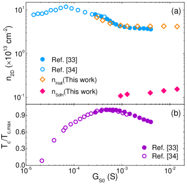
Figure 1: Gate dependence of transport parameters. (a) The sheet carrier density ($n_{\text{2D}}$) determined from low-field Hall measurements and quantum oscillations as a function of the zero field sheet conductance ($G_{\text{S0}}$). (b) Normalized superconducting critical temperature $T_{\text{c}}/T_{\text{c,max}}$ as a function of $G_{\text{S0}}$.

Transport measurements.— $14$ monolayer thick epitaxial thin film of LaAlO₃ were grown on atomically flat Ti-terminated SrTiO₃ $(111)$ substrate using the pulsed laser deposition technique in combination with reflection high energy electron diffraction. Details of the deposition procedure and substrate treatment are described in Ref. Rout et al. (2017a). Electrical transport measurements of the $80$ $\mu\text{m}\times 260$ $\mu\text{m}$ Hall bar, patterned along the [1$\bar{2}$1] direction using optical lithography Rout et al. (2017a), were performed by a four probe ac technique with a current of $50$ nA in a custom made ³He cryostat equipped with a $35$ T magnet.

We investigated magnetotransport at the $(111)$ interface under a perpendicular field to understand the behavior of the carrier density ($n_{\text{2D}}$) as a function of temperature ($T$) and gate voltage ($V_{\text{g}}$) in a back-gated device. $n_{\text{2D}}$ was extracted using both the Hall density [$n_{\text{Hall}}=(e{R_{\text{H}}})^{-1}$, where $R_{\text{H}}$ is the slope of the low-field Hall resistivity] and the Shubnikov-de Haas (SdH) oscillations (through the Onsager relation sup ) observed at higher magnetic fields. We also studied corresponding variation of the superconducting transition temperature. The back-gate was employed to control the carrier density and vary the sheet conductance ($G_{\text{S}}$). Since the gate response changes between different sample cool-downs and $V_{\text{g}}$ sweeps, we present the results in Fig. 1 as a function of the zero field conductance $G_{\text{S0}}$ Mograbi et al. (2018). The $V_{\text{g}}$ dependence can be found in sup .

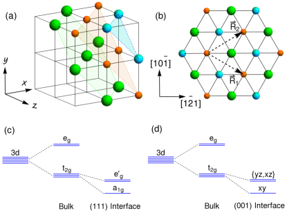
Figure 2: Crystal structure of the $(111)$ LaAlO₃/SrTiO₃ interface. (a) Three inequivalent layers of Ti atoms ($\text{green }\equiv\text{Ti}_{1}\text{, orange}\equiv\text{Ti}_{2}\text{, blue}\equiv\text{Ti}_{3}$) forming one unit cell at the $(111)$ interface of a cubic lattice. (b) Top view of the $(111)$ trilayer. $\vec{R}_{1,2}$ are the lattice vectors of the triangular lattice at the interface. (c),(d) Level structure of the Ti 3d-orbitals at the $(111)$ and $(001)$ interfaces, respectively. The bulk cubic structure leads to the splitting into t${}_{\text{2g}}$ and e${}_{\text{g}}$ orbitals. (c) The trigonal crystal symmetry at the $(111)$ interface leads to further splitting of t${}_{\text{2g}}$ into a${}_{\text{1g}}$ and e${}_{\text{g}}^{\prime}$ orbitals. (d) The in-plane crystal symmetry does not change at the $(001)$ interface but the surface confinement lifts the degeneracy.

Fig. 1(a) compares the variation of carrier density from the SdH analysis ($n_{\text{SdH}}$) and the Hall measurement ($n_{\text{Hall}}$) with the gate voltage ($V_{\text{g}}$), while Fig. 1(b) presents the corresponding dependence of the superconducting critical temperature ($T_{\text{c}}$). The observed variation and values of $n_{\text{Hall}}$ are consistent with our previous results on the $(111)$ interface Mograbi et al. (2018); Rout et al. (2017b) [also shown in Fig. 1(a)] and with other recent results Davis et al. (2017); Monteiro et al. (2018).

Curiously, we find that while $n_{\text{Hall}}$ and $T_{\text{c}}$ are non-monotonic functions of $V_{\text{g}}$, $n_{\text{SdH}}$ changes monotonically. Moreover, the peak in $n_{\text{Hall}}$ appears when quantum oscillations are not observable. These features are strikingly different from our previous measurements on the $(001)$ interface Maniv et al. (2015). In the latter case, $n_{\text{SdH}}$ also changes non-monotonically with $V_{\text{g}}$ and the maximal $n_{\text{SdH}}$, $n_{\text{Hall}}$, and $T_{\text{c}}$ appear at roughly the same gate voltage.

At both interfaces $n_{\text{SdH}}$ is much smaller than $n_{\text{Hall}}$. Since the SdH signal decays exponentially with inverse scattering time, this indicates the presence of two low-energy bands in the electronic structure with different mobilities. Therefore, both bands would contribute to $n_{\text{Hall}}$ but only the mobile one would be observable through the quantum oscillation measurements.

We note that the band structure of $(111)$ LaAlO₃/SrTiO₃ has recently been probed using Hall measurements Monteiro et al. (2018). However, the Hall coefficient receives contributions from all the bands and also depends on the corresponding scattering times, making it hard to decipher the band structure. The crucial new ingredient here is the quantum oscillations, which directly probe the population of the more mobile band, and demonstrate the qualitative difference between the $(111)$ and $(001)$ interfaces. These allow us to develop a complete and consistent theoretical picture for both interfaces, as we now turn to describe.

Theoretical Model.— We first consider the orbital character of the relevant levels at the two interfaces. Ab-initio studies Santander-Syro et al. (2011); Popović et al. (2008); Delugas et al. (2011) show that the low energy conduction bands in bulk SrTiO₃ are composed of the t${}_{\text{2g}}$ orbitals of the Ti atoms. These are degenerate in the bulk due to their cubic arrangement (the low temperature structural distortions are negligible for our purposes), which imparts octahedral symmetry to the band structure. However, the reduced symmetry at the interfaces can lift the degeneracy and modify the orbital character.

At the $(001)$ interface, Ti atoms form a square lattice, which does not modify the in-plane crystal-field. In combination with the confining potential, the degeneracy of the t${}_{\text{2g}}$ orbitals is lifted but the orbital character is not modified. Specifically, if the confinement is along the $z$ direction, then the $xy$ orbital is lowered in energy due to its higher effective mass in the confinement direction Santander-Syro et al. (2011) [Fig. 2(d)]. On the other hand, at the $(111)$ interface, Ti atoms form a stacked triangular lattice with three interlaced layers [Fig. 2(a),(b)]. This changes the bulk octahedral symmetry to triangular at the interface and introduces a new in-plane crystal field Khomskii (2014), which hybridizes the t${}_{\text{2g}}$ orbitals, forming $|a_{\text{1g}}\rangle=(|xy\rangle+|yz\rangle+|xz\rangle)/\sqrt{3}$ and $|e_{\text{g}\pm}^{\prime}\rangle=(|xy\rangle+\omega^{\pm 1}|yz\rangle+\omega^{\pm 2}|xz\rangle)/\sqrt{3}$ where $\omega=e^{2\pi i/3}$. Their splitting is sensitive to details of the interface. Here, we choose parameters such that a${}_{\text{1g}}$ is lower in energy [Fig. 2(c)], in accordance with recent XLD experiments De Luca et al. (2018) and DFT calculations Doennig et al. (2013); Beltrán and Muñoz (2017).

Next, we employ a tight-binding model with these orbitals on the first three inequivalent layers [Fig. 2(a)], keeping track of the separation and connectivity of sites on the different layers fnL . In the basis, $\{|a_{\text{1g}}\rangle,|e^{\prime}_{\text{g}+}\rangle,|e^{\prime}_{\text{g}-}\rangle\}\otimes\{|\text{Ti}_{1}\rangle,|\text{Ti}_{2}\rangle,|\text{Ti}_{3}\rangle\}\otimes\{|{\uparrow}\rangle,|{\downarrow}\rangle\}$, the hopping terms can be written as $18\times 18$ matrices given by

$$H^{(111)}_{\text{0}}(\vec{K})=\left(\begin{array}[]{ccc}A(\vec{K})&B(\vec{K})&B^{\dagger}(\vec{K})\\ B^{\dagger}(\vec{K})&A(\vec{K})&B(\vec{K})\\ B(\vec{K})&B^{\dagger}(\vec{K})&A(\vec{K})\end{array}\right)\otimes\mathcal{I}_{2},$$ (4)

where, the block matrices $A(\vec{K})$ and $B(\vec{K})$ are,

$$A(\vec{K}) =-\frac{(2t+t^{\prime})}{3}\left(\begin{array}[]{ccc}0&e^{-iK_{2}}f_{0}(\vec{K})&0\\ e^{iK_{2}}f_{0}(-\vec{K})&0&e^{-iK_{1}}f_{0}(\vec{K})\\ 0&e^{iK_{1}}f_{0}(-\vec{K})&0\end{array}\right)-\frac{t^{\prime\prime}}{3}\left(\begin{array}[]{ccc}2\epsilon_{0}(\vec{K})&0&f_{0}(-\vec{K})\\ 0&2\epsilon_{0}(\vec{K})&0\\ f_{0}(\vec{K})&0&2\epsilon_{0}(\vec{K})\end{array}\right),$$ (11)

$$B(\vec{K}) =\omega^{2}\frac{(t-t^{\prime})}{3}\left(\begin{array}[]{ccc}0&e^{-iK_{2}}f_{\omega}(\vec{K})&0\\ e^{iK_{2}}f_{\omega}(-\vec{K})&0&e^{-iK_{1}}f_{\omega}(\vec{K})\\ 0&e^{iK_{1}}f_{\omega}(-\vec{K})&0\end{array}\right)-\omega^{2}\frac{t^{\prime\prime}}{3}\left(\begin{array}[]{ccc}2\epsilon_{\omega}(\vec{K})&0&f_{\omega}(-\vec{K})\\ 0&2\epsilon_{\omega}(\vec{K})&0\\ f_{\omega}(\vec{K})&0&2\epsilon_{\omega}(\vec{K})\end{array}\right),$$ (18)

where, $t$ and $t^{\prime}$ are the light and heavy nearest neighbor hopping amplitudes while $t^{\prime\prime}$ is the next-nearest neighbor hopping. $f_{0}(\vec{K})=1+e^{iK_{1}}+e^{iK_{2}}$, $f_{\omega}(\vec{K})=1+\omega e^{iK_{1}}+\omega^{2}e^{iK_{2}}$, $\epsilon_{0}(\vec{K})=\cos(K_{1})+\cos(K_{2})+\cos(K_{1}-K_{2})$ and $\epsilon_{\omega}(\vec{K})=\cos(K_{1}-K_{2})+\omega\cos(K_{2})+\omega^{2}\cos(K_{1})$, where $K_{1,2}\in[-\pi,\pi]$, the two-dimensional Brillouin zone. The atomic spin-orbit coupling is an on-site term mixing the orbitals and spin states. Taking the spin quantization axis along the $(111)$ direction, the spin-orbit coupling is,

$$H^{(111)}_{\text{SO}}=\frac{\Delta_{\text{so}}}{2}\left(\begin{array}[]{ccc}0&-\sqrt{2}\sigma^{+}&\sqrt{2}\sigma^{-}\\ -\sqrt{2}\sigma^{-}&-\sigma_{z}&0\\ \sqrt{2}\sigma^{+}&0&\sigma_{z}\end{array}\right),$$ (22)

where $\sigma^{\pm}=(\sigma_{x}\pm i\sigma_{y})/2$, with $\sigma_{x,y,z}$ being the Pauli matrices. Additionally, the single-particle Hamiltonian includes the trigonal crystal-field $\Delta_{\text{cf}}$ (which lifts the degeneracy between the orbitals) and a linear confining potential $V_{\text{c}}$ (which lifts the layer degeneracy) sup .

Finally, correlation effects are incorporated through an on-site Hubbard term $\sum_{\text{r}}\sum_{\text{I}\neq\text{J}}Un_{\text{rI}}n_{\text{rJ}}$, which includes both inter-orbital and intra-orbital repulsion (assumed to be of equal strength in order to reduce the number of free parameters). The two-body term is then treated in the Hartree-Fock approximation. The mean-field ansatz is that the ground state is invariant under time-reversal and has the full symmetry of the (interface) crystal structure, i.e. the C_3v group at the $(111)$ interface (we have verified that tetragonal distortions etc. have a small effect on our results). Under this assumption, the Hubbard term reduces to a one-body term with four independent real parameters (per layer) — the occupancy of the three orbitals (which appear in the Hartree terms) and one spin-mixing average (Fock term) which renormalizes the spin-orbit interaction. We note that a state with the full crystal symmetry must have equal occupancy of the $xy$, $yz$ and $xz$ orbitals. Therefore, in terms of the original t${}_{\text{2g}}$ orbitals, there is only one independent Hartree term and three Fock terms.

The mean-field Hamiltonian is solved self-consistently, using $t=V_{\text{c}}=437.5$ meV, $t^{\prime}=t^{\prime\prime}=20$ meV, $\Delta_{\text{so}}=3$ meV, $\Delta_{\text{cf}}=2$ meV and $U=2$ eV. These parameter values are close to those employed previously for the $(001)$ interface Joshua et al. (2012); Ruhman et al. (2014); Maniv et al. (2015, 2017). Although surface reconstruction can lead to different parameters at the two interfaces, the qualitative behavior is not expected to change.

Theoretical Results.— Fig. 3 shows the results of the self-consistent calculation for the $(111)$ interface. Figs. 3(a),(b) show the dispersion of the two lowest energy bands at two different chemical potentials ($\mu$) and Figs. 3(c),(d) show the corresponding Fermi contours. For small values of $\mu$, only the lowest band is occupied. Close to the $\Gamma$ point, it mostly consists of the a${}_{\text{1g}}$ orbital. Away from $\Gamma$, the orbital character changes and becomes anisotropic. At larger $\mu$, the second band is also populated [Figs. 3(b),(d)]. For the range of $\mu$ relevant here, this band consists primarily of one of the e${}_{\text{g}}^{\prime}$ orbitals and remains almost parabolic. Crucially, Fig. 3(e) shows the monotonic variation of carrier density of the two bands as a function of $\mu$. The monotonic rise of the second band population agrees quite well with the SdH data [Fig. 1(a)], and supports our assumption that only this band gives rise to visible quantum oscillations, due to its higher mobility.

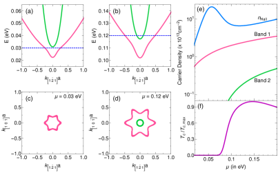
Figure 3: Results of the theoretical model for the $(111)$ interface. (a),(b) Band structure for two different chemical potentials $\mu$ before ($\mu$ = 0.03 eV) and after ($\mu$ = 0.12 eV) the second band starts getting occupied. The pink (green) line corresponds to band 1 (2), which is composed of a${}_{\text{1g}}$ (e${}_{\text{g}}^{\prime}$) orbitals close the $\Gamma$ point. The dashed blue line marks the Fermi energy. (c),(d) show the Fermi contours corresponding to the band structures in (a),(b) respectively. The outer surface (corresponding to band 1) is highly anisotropic at all $\mu$. (e) The carrier and Hall densities as a function of $\mu$. The carrier density is monotonic for both bands, while the Hall density is non-monotonic. The peak in $n_{\text{Hall}}$ occurs before the second band starts getting populated. This is in accordance with the experiment (Fig. 1) and indicates that it is due to the anisotropic shape of the lowest band. (f) Normalized superconducting critical temperature ($T_{\text{c}}/T_{\text{c,max}}$) as a function of $\mu$ within the single-band BCS model.

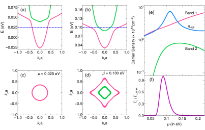
Figure 4: Results of the theoretical model at $(001)$ interface. (a),(b) Bandstructure for two different chemical potentials $\mu$ before ($\mu$ = 0.025 eV) and after ($\mu$ = 0.10 eV) the second band starts getting occupied. The pink (green) line corresponds to band 1 (2), which is composed of $xy$ (other t_2g) orbitals close to the $\Gamma$ point. The dashed blue line marks the Fermi energy. (c),(d) show the Fermi contours corresponding to the band structures in (a),(b) respectively. The outer surface (corresponding to band 1) is isotropic at low values of $\mu$. When the second band gets populated, the orbital character of the bands switches and the outer band becomes anisotropic. (e) The carrier and Hall densities as a function of $\mu$. The carrier density for second band is non-monotonic due to correlation-induced transfer of electrons from the lighter to heavier band. The Hall density is non-monotonic due to the anisotropy in the Fermi contour of the bands. (f) Normalized superconducting critical temperature ($T_{\text{c}}/T_{\text{c,max}}$) as a function of $\mu$ within the single-band BCS model.

Upon increasing gate voltage the measured $n_{\text{Hall}}$ [Fig. 1(a)] has a peak before the quantum oscillations are visible. This means that this observed non-monotonicity must arise from the lowest band by itself. This is an important difference between the $(001)$ and the $(111)$ interfaces that can be identified here because of our combination of SdH and Hall measurements. Figs. 3(c),(d) show that the first band is non-parabolic and consists of regions with both positive and negative curvature, throughout the range of relevant chemical potential. This implies that a wavepacket gliding around the constant energy surface will give both electron-like and hole-like contributions to the Hall conductivity. This is further complicated by the momentum-dependent orbital character of the band at large filling. Under these conditions, the standard Drude relation between inverse Hall coefficient and the carrier density of a single band $[n_{\text{b}}=(eR_{\text{H}})^{-1}]$ is no longer valid and $n_{\text{Hall}}$ can differ significantly from the actual band population. Similarly the two band model, often used to fit Hall data for oxide interfaces, is valid only in case of two isotropic bands with no orbital mixing and therefore is not directly applicable for $(111)$ LaAlO₃/SrTiO₃.

To properly account for these features we compute the longitudinal and Hall conductivity ($\sigma_{\text{L}}$ and $\sigma_{\text{H}}$) using general expressions derived from the Boltzmann equation assuming momentum dependent scattering times sup ; Ong (1991); Hurd (1972). Specifically, we fix the orbital lifetimes ($\tau_{\text{a}_{\text{1g}}}$ and $\tau_{\text{e}_{\text{g}\pm}^{\prime}}$) and assume the scattering time for $m$th band to be, $\tau_{m}(\vec{K})=\sum_{\sigma}\tau_{\text{a}_{\text{1g}}}|\psi_{m}(\text{a}_{\text{1g}},\sigma,\vec{K})|^{2}+\tau_{\text{e}_{\text{g}}^{\prime}}\big{(}|\psi_{m}(\text{e}_{\text{g}+}^{\prime},\sigma,\vec{K})|^{2}+|\psi_{m}(\text{e}_{\text{g}-}^{\prime},\sigma,\vec{K})|^{2}\big{)}$, where $\psi_{m}$ is the self-consistent wavefunction for the $m$th band. This allows $\tau_{m}(\vec{K})$ to trace the changes in orbital character along the Fermi contours. Here we choose $\tau_{\text{e}_{\text{g}}^{\prime}}=10\tau_{\text{a}_{\text{1g}}}$, so that the second band is more mobile. While $\sigma_{\text{L}}$ and $\sigma_{\text{H}}$ depend on the orbital lifetimes separately, and are thus harder to constrain by experimental data, $n_{\text{Hall}}$ ($\approx\sigma_{\text{L}}^{2}/\sigma_{\text{H}}$) depends only on the ratio of the lifetimes. Therefore we show the variation of $n_{\text{Hall}}$ as a function of $\mu$ in Fig. 3(e). The decent agreement of this theoretical result with experimental data from Fig. 1(a) implies that the experimental observations are a consequence of the shape and orbital character of the lowest band.

We note that the Fermi contours in Fig. 3(c),(d) are similar to those reported for the $(111)$ surface of SrTiO₃ Rödel et al. (2014). However, unlike the band structure in Fig. 3(a),(b) Ref. Rödel et al. (2014) did not observe any splitting between the two lowest bands. This difference stems from the change in order of a${}_{\text{1g}}$ and e${}_{\text{g}}^{\prime}$ bands between the SrTiO₃ surface and LaAlO₃/SrTiO₃ interface Doennig et al. (2013); Beltrán and Muñoz (2017); De Luca et al. (2018). In our model, this order is fixed by the sign of $\Delta_{\text{cf}}$, which we choose in accordance with Ref. De Luca et al. (2018). Using the opposite sign would provide a band structure similar to the one reported in Ref. Rödel et al. (2014).

Fig. 4 shows the results of a similar calculation for the $(001)$ interface using a closely related model Maniv et al. (2015, 2017). Figs. 3(e) and 4(e) markedly differ in the behavior of the carrier density of band 2 at the two interfaces: Here the population of band 2 ($n_{\mathrm{SdH}}$) is nonmonotonic, and the Hall density follows it [as opposed to monotonic SdH and maximal Hall number when band 2 is empty in $(111)$]. We stress that the nonmonotonic behavior of band 2 population at the $(001)$ interface [Fig. 4(e)] is not due to larger interaction terms (the three largest parameters, $U$, $t$, and $t^{\prime}$, were taken to be equal in both cases). Rather it occurs because at the $(001)$ interface the bands retain their original orbital characters ($xy$, $yz$ and $xz$), which have a large difference in effective mass in the interface plane. This generates a correlation-induced population transfer among the bands, because the total energy can be minimized by transferring electrons from the lighter to heavier band Maniv et al. (2015, 2017); Smink et al. (2017). Since band 2 changes from heavy to light with increasing $\mu$ [Fig. 4(a),(b)], it is first populated then depopulated. In contrast, at the $(111)$ interface, all three t${}_{\text{2g}}$ orbitals contribute equally to both bands, and thus the effective band masses are not different enough for correlations to induce population transfer. The nonmonotonic $n_{\mathrm{Hall}}$ in $(111)$ is rather the result of the greater Fermi contour curvature induced by the triangular symmetry, as compared to the square symmetry at $(001)$.

Finally, while our model does not account for the origin of superconductivity, we attempt to estimate the superconducting critical temperature for our band structure using the single-band BCS expression, $T_{\text{c}}=1.13T_{\theta}\exp(-\frac{1}{\rho_{2}V_{\text{BCS}}})$ Tinkham (2004). Here we assume that the mobile band 2 has a higher contribution to the superconductivity, and therefore use its density of states ($\rho_{2}$). $T_{\theta}$ is the Debye temperature of SrTiO₃ Burns (1980), and $V_{\mathrm{BCS}}$ is set so that $T_{\text{c}}$ matches the experimental value at the maximum. Figs. 3(f) and 4(f) show that we get good fits for the relative positions peaks in $T_{\text{c}}$ and $n_{\text{Hall}}$ with this simplistic model.

Conclusions.— We measured the variation of quantum oscillations frequency, Hall signal, and superconducting $T_{\text{c}}$ with gate voltage in $(111)$ LaAlO₃/SrTiO₃ and found it to be qualitatively different from the $(001)$ interface. Employing a tight-binding model with on-site correlations, we calculated the band structure at both interfaces and showed that the difference in the crystal structure leads to bands with different orbital character. In $(001)$ interface correlation-induced population transfer is the primary mechanism for the nonmonotonicity, while in $(111)$ it is the shape of the symmetry-induced Fermi contours. This sets the stage for future investigation of the effect of this peculiar band structure on the superconductivity, magnetism, and ferroelectricity in these and related interfaces.

Supplemental material for “Symmetry and correlation effects on band structure explain the anomalous transport properties of $(111)$ LaAlO₃/SrTiO₃”

S1 I.       Structure and Symmetry of the $(111)$ interface

As described in the main text, the low-energy conduction bands in bulk SrTiO₃ are composed of the t${}_{\text{2g}}$ orbitals of Ti, which form a cubic structure (neglecting the structure distortions at low temperatures). Fig. S1 shows that the projection of a cube into a plane normal to the $(111)$ direction is a stack of triangular lattices with 3 inequivalent sites (labelled as Ti_i). The new (in-plane) lattice vectors are

$$\vec{R}_{\text{1,2}} =\sqrt{2}a\left(\frac{\sqrt{3}}{2}\hat{X}\mp\frac{\hat{Y}}{2}\right),$$ (S1)

where $a$ is the lattice constant (of the cubic lattice) and $\hat{X},\hat{Y}$ are unit vectors along the $[1\bar{2}1],[10\bar{1}]$ directions, respectively. We also define $\hat{Z}$ as the $[111]$ direction. The change in crystal structure (from cubic to triangular) introduces a new (in-plane) crystal field at the interface, which lifts the degeneracy of the t${}_{\text{2g}}$ orbitals and mixes them to form,

$$|\text{a}_{\text{1g}}\rangle =\frac{1}{\sqrt{3}}\big{[}|xy\rangle+|yz\rangle+|xz\rangle\big{]},$$ (S2)

$$|\text{e}_{\text{g}+}^{\prime}\rangle =\frac{1}{\sqrt{3}}\big{[}|xy\rangle+\omega|yz\rangle+\omega^{2}|xz\rangle\big{]},$$ (S3)

$$|\text{e}_{\text{g}-}^{\prime}\rangle =\frac{1}{\sqrt{3}}\big{[}|xy\rangle+\omega^{-1}|yz\rangle+\omega^{-2}|xz\rangle\big{]},$$ (S4)

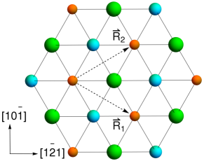
Figure S1: Projection of a cubic lattice onto the plane normal to the $(111)$ direction. A unit cell with 3 inequivalent sites (denoted by green $\equiv\text{Ti}_{1}$, orange $\equiv\text{Ti}_{2}$ and blue $\equiv\text{Ti}_{3}$) forms a triangular lattice stacked along the $\hat{Z}$ direction. $\vec{R}_{\text{1}}$ and $\vec{R}_{\text{2}}$ are the new (in-plane) lattice vectors for the triangular lattice.

where $\omega=e^{i\frac{2\pi}{3}}$ is the cubic root of unity. Below we describe how these orbitals behave under the symmetry transformations relevant to this system.

Spatial Symmetries

The triangular lattice formed by $\big{(}\vec{R}_{1},\vec{R}_{2}\big{)}$ is invariant under the C_3v group, which can be generated by two operators:

1. Rotation about $\hat{Z}$ by $\frac{2\pi}{3}$ : The $|\text{a}_{\text{1g}}\rangle$ orbital is invariant under this transformation, while the others pick up a phase,

$$|\text{e}_{\text{g}\pm}^{\prime}\rangle\rightarrow\omega^{\pm 2}|\text{e}_{\text{g}\pm}^{\prime}\rangle.$$ (S5)

Similarly, choosing $\hat{Z}$ as the spin quantization axis, the spin states transform as,

$$\{|{\uparrow}\rangle,|{\downarrow}\rangle\}\rightarrow\{-\omega|{\uparrow}\rangle,-\omega^{-1}|{\downarrow}\rangle\}.$$ (S6)

2. Reflection about $\hat{X}-\hat{Z}$ plane : Reflection can be thought of as inversion about the origin followed by a rotation of $\pi$ about $\hat{Y}$. Again, $|\text{a}_{\text{1g}}\rangle$ is invariant under such a reflection, while the other states transform into each other,

$$|\text{e}_{\text{g}\pm}^{\prime}\rangle\rightarrow\omega^{\pm 1}|\text{e}_{\text{g}\mp}^{\prime}\rangle.$$ (S7)

Similarly, the spin states are also exchanged,

$$\{|{\uparrow}\rangle,|{\downarrow}\rangle\}\rightarrow\{\omega^{-1}|{\downarrow}\rangle,-\omega|{\uparrow}\rangle\}.$$ (S8)

Time-Reversal

The time-reversal operator involves complex conjugation followed by a rotation of the spins by $\pi$ along some axis. We choose to rotate along $-\frac{\sqrt{3}}{2}\hat{X}-\frac{\hat{Y}}{2}$ so that the spin states transform (under time-reversal) as,

$$\{|{\uparrow}\rangle,|{\downarrow}\rangle\}\rightarrow\{|{\downarrow}\rangle,-|{\uparrow}\rangle\}.$$ (S9)

The orbital states are eigenstates of $\hat{L}_{Z}$ (angular momentum along $\hat{Z}$) and hence also transform under time-reversal. The a${}_{\text{1g}}$ corresponds to $m=0$ and is therefore invariant, while the others (corresponding to $m=\pm 1$) transform as,

$$|\text{e}_{\text{g}\pm}^{\prime}\rangle\rightarrow|\text{e}_{\text{g}\mp}^{\prime}\rangle.$$ (S10)

Constraints on one-body matrix elements

In this work, we assume that the final ground state of the system is invariant under translations (by $\vec{R}_{1,2}$), time-reversal and all the spatial symmetries of the crystal structure ($C_{3v}$). This invariance introduces some constraints on the (on-site) one-body matrix elements,

$$V_{\sigma\sigma^{\prime}}^{mm^{\prime}}(\vec{R},i)=\langle c^{\dagger}_{im\sigma}(\vec{R})c_{im^{\prime}\sigma^{\prime}}(\vec{R})\rangle,$$ (S11)

where $\vec{R}$ is the position of the unit cell, $i$ labels the different atoms (Ti_i) of the unit cell, $m,m^{\prime}$ are the on-site orbitals ($\text{a}_{\text{1g}},\text{e}_{\text{g}\pm}^{\prime}$) and $\sigma,\sigma^{\prime}$ are the spin states. We use these constraints to simplify the mean-field ansatz. Since the two-body term involved in our calculation is an on-site term, we do not need the constraints on other matrix elements.

Due to translation symmetry, the matrix elements are independent of $\vec{R}$ (but not of $i$). We note that the transformations considered here only mix states on a given site ($i$) of the unit cell, i.e., $i$ does not change under the symmetry operations described below.

1. Time-Reversal : For a system invariant under time-reversal ($\mathcal{T}$), the matrix elements must satisfy,

$$\langle\psi|\phi\rangle=\langle\tilde{\phi}|\tilde{\psi}\rangle=\langle\tilde{\psi}|\tilde{\phi}\rangle^{*},$$ (S12)

where $|\tilde{\psi}\rangle=\mathcal{T}|\psi\rangle$ and $|\tilde{\phi}\rangle=\mathcal{T}|\phi\rangle$. This implies that due to time-reversal symmetry,

$$V_{\sigma\sigma^{\prime}}^{mm^{\prime}}(i)=\pm V_{\tilde{\sigma}^{\prime}\tilde{\sigma}}^{\tilde{m}^{\prime}\tilde{m}}(i),$$ (S13)

where the $+$ ($-$) sign appears if $\sigma=\sigma^{\prime}$ (otherwise), $\tilde{\sigma}$ is the spin state opposite to $\sigma$ and $\tilde{m}$ is the orbital state related to $m$ as described in equation (S10). This means that the occupancies of several levels are related to each other,

$$V_{{\uparrow}{\uparrow}}^{\text{a}_{\text{1g}}\text{a}_{\text{1g}}}(i) =V_{{\downarrow}{\downarrow}}^{\text{a}_{\text{1g}}\text{a}_{\text{1g}}}(i)=N_{\text{a}_{\text{1g}}}(i),$$ (S14)

$$V_{{\uparrow}{\uparrow}}^{\text{e}_{\text{g}+}^{\prime}\text{e}_{\text{g}+}^{\prime}}(i) =V_{{\downarrow}{\downarrow}}^{\text{e}_{\text{g}-}^{\prime}\text{e}_{\text{g}-}^{\prime}}(i)=N_{\text{e}_{\text{g}+}^{\prime}}(i),$$ (S15)

$$V_{{\uparrow}{\uparrow}}^{\text{e}_{\text{g}-}^{\prime}\text{e}_{\text{g}-}^{\prime}}(i) =V_{{\downarrow}{\downarrow}}^{\text{e}_{\text{g}+}^{\prime}\text{e}_{\text{g}+}^{\prime}}(i)=N_{\text{e}_{\text{g}-}^{\prime}}(i).$$ (S16)

Additionally, the following matrix elements must necessarily vanish (for all $i$),

$$V_{{\uparrow}{\downarrow}}^{\text{a}_{\text{1g}}\text{a}_{\text{1g}}}=\, 0=V_{{\downarrow}{\uparrow}}^{\text{a}_{\text{1g}}\text{a}_{\text{1g}}},$$ (S17)

$$V_{{\uparrow}{\downarrow}}^{\text{e}_{\text{g}+}^{\prime}\text{e}_{\text{g}-}^{\prime}}=\, 0=V_{{\downarrow}{\uparrow}}^{\text{e}_{\text{g}+}^{\prime}\text{e}_{\text{g}-}^{\prime}},$$ (S18)

$$V_{{\uparrow}{\downarrow}}^{\text{e}_{\text{g}-}^{\prime}\text{e}_{\text{g}+}^{\prime}}=\, 0=V_{{\downarrow}{\uparrow}}^{\text{e}_{\text{g}-}^{\prime}\text{e}_{\text{g}+}^{\prime}}.$$ (S19)

2. Rotations : Using equations (S5) and (S6) we find that invariance under rotations forces yet more matrix elements to vanish (at all $i$),

$$V_{{\uparrow}{\downarrow}}^{\text{e}_{\text{g}s}^{\prime}\text{e}_{\text{g}s}^{\prime}}=\, 0=V_{{\downarrow}{\uparrow}}^{\text{e}_{\text{g}s}^{\prime}\text{e}_{\text{g}s}^{\prime}},$$ (S20)

$$V_{\sigma\sigma}^{\text{e}_{\text{g}+}^{\prime}\text{e}_{\text{g}-}^{\prime}}=\, 0=V_{\sigma\sigma}^{\text{e}_{\text{g}-}^{\prime}\text{e}_{\text{g}+}^{\prime}},$$ (S21)

$$V_{\sigma\sigma}^{\text{a}_{\text{1g}}\text{e}_{\text{g}s}^{\prime}}=\, 0=V_{\sigma\sigma}^{\text{e}_{\text{g}s}^{\prime}\text{a}_{\text{1g}}},$$ (S22)

$$V_{{\uparrow}{\downarrow}}^{\text{a}_{\text{1g}}\text{e}_{\text{g}-}^{\prime}}=\, 0=V_{{\uparrow}{\downarrow}}^{\text{e}_{\text{g}+}^{\prime}\text{a}_{\text{1g}}},$$ (S23)

$$V_{{\downarrow}{\uparrow}}^{\text{a}_{\text{1g}}\text{e}_{\text{g}+}^{\prime}}=\, 0=V_{{\downarrow}{\uparrow}}^{\text{e}_{\text{g}-}^{\prime}\text{a}_{\text{1g}}}.$$ (S24)

for all $s=\pm$ and $\sigma={\uparrow},{\downarrow}$.

3. Reflections : The only non-zero matrix elements with different spin states are related to each other through the following sequence of operations (again at all $i$),

$$V_{{\uparrow}{\downarrow}}^{\text{a}_{\text{1g}}\text{e}_{\text{g}+}^{\prime}} =-V_{{\uparrow}{\downarrow}}^{\text{e}_{\text{g}-}^{\prime}\text{a}_{\text{1g}}}\,\,\text{ by time-reversal invariance}$$

$$=-\big{(}V_{{\downarrow}{\uparrow}}^{\text{a}_{\text{1g}}\text{e}_{\text{g}-}^{\prime}}\big{)}^{*}\,\,\text{ by hermitian-conjugation}$$

$$=-\big{(}-V_{{\uparrow}{\downarrow}}^{\text{a}_{\text{1g}}\text{e}_{\text{g}+}^{\prime}}\big{)}^{*}\,\,\text{ due to reflection invariance}$$

$$=\big{(}V_{{\uparrow}{\downarrow}}^{\text{a}_{\text{1g}}\text{e}_{\text{g}+}^{\prime}}\big{)}^{*}.$$ (S25)

The last line implies that these matrix elements are all real. Then we define the only spin-mixing average allowed by symmetry as

$$N_{\text{SO}}(i)=V_{{\uparrow}{\downarrow}}^{\text{a}_{\text{1g}}\text{e}_{\text{g}+}^{\prime}}(i)=-V_{{\downarrow}{\uparrow}}^{\text{a}_{\text{1g}}\text{e}_{\text{g}-}^{\prime}}(i).$$ (S26)

Therefore, the crystal structure at the $(111)$ interface allows only four (real and independent) one-body matrix elements (per layer) : $N_{\text{a}_{\text{1g}}}(i)$, $N_{\text{e}_{\text{g}+}^{\prime}}(i)$, $N_{\text{e}_{\text{g}-}^{\prime}}(i)$, and $N_{\text{SO}}(i)$.

S2 II.       Hamiltonian and conductivity at the $(111)$ interface

As described above, the $(111)$ interface of SrTiO₃/LaAlO₃ has a triangular crystal structure with a complex unit cell (cf. Fig. S1). In order to correctly represent the connectivity of the different Ti atoms (in the underlying cubic lattice), we first write a Hamiltonian for the bulk and then adapt it to describe the interface.

Bulk Hamiltonian

In the bulk, we employ a tight-binding Hamiltonian based on a model of Refs. Bistritzer et al. (2011); Khalsa and MacDonald (2012). It can be written as $H_{\text{b}}(\vec{k})=H_{\text{0}}(\vec{k})+H_{\text{SO}}$, where $H_{\text{SO}}=\Delta_{\text{SO}}\vec{L}\cdot\vec{s}$ is the atomic spin-orbit (SO) coupling and $H_{\text{0}}(\vec{k})$ is the kinetic term composed of nearest-neighbor (NN) hopping.

We express $H_{\text{b}}$ in terms of the a${}_{\text{1g}}$ and e${}_{\text{g}\pm}^{\prime}$ orbitals and use $\hat{Z}$ as the spin-quantization axis on the trilayer triangular lattice (Fig. S1), which is equivalent to the cubic lattice. The three lattice vectors for this structure are $\vec{R}_{1,2}$ defined in Eq. (S1) and $\vec{R}_{3}=\sqrt{3}a\hat{Z}$. The three-dimensional Brillouin zone is defined by the reciprocal lattice vectors, $\vec{G}_{1,2}=\frac{\sqrt{2}}{\sqrt{3}a}\left(\frac{\hat{K}_{X}}{2}\mp\frac{\sqrt{3}}{2}\hat{K}_{Y}\right)$ and $\vec{G}_{3}=\frac{1}{\sqrt{3}a}\hat{K}_{Z}$. To avoid confusion, we denote the three-dimensional (bulk) momentum by $\vec{k}=(k_{1},k_{2},k_{3})$ and the two-dimensional surface momentum by $\vec{K}=(K_{1},K_{2})$, with $k_{a},K_{a}\in[-\pi,\pi]$. Labelling the three layers as $i=1,2,3$, we can write the NN term as an 18$\times$18 matrix in the basis, $\{|a_{\text{1g}}\rangle,|e^{\prime}_{\text{g}+}\rangle,|e^{\prime}_{\text{g}-}\rangle\}\otimes\{|\text{Ti}_{1}\rangle,|\text{Ti}_{2}\rangle,|\text{Ti}_{3}\rangle\}\otimes\{|{\uparrow}\rangle,|{\downarrow}\rangle\}$ as

$$H_{\text{0}}(\vec{k})=\left(\begin{array}[]{ccc}\tilde{A}_{2}(\vec{k})&\tilde{B}_{2}(\vec{k})&\tilde{B}_{2}^{\dagger}(\vec{k})\\ \tilde{B}_{2}^{\dagger}(\vec{k})&\tilde{A}_{2}(\vec{k})&\tilde{B}_{2}(\vec{k})\\ \tilde{B}_{2}(\vec{k})&\tilde{B}_{2}^{\dagger}(\vec{k})&\tilde{A}_{2}(\vec{k})\end{array}\right)\otimes\mathcal{I}_{2},$$ (S30)

where the block matrices $\tilde{A}_{2}(\vec{k})$ and $\tilde{B}_{2}(\vec{k})$ are,

$$\tilde{A}_{2}(\vec{k}) =-\frac{(2t+t^{\prime})}{3}\left(\begin{array}[]{ccc}0&e^{-ik_{2}}f_{0}(\vec{k})&e^{-ik_{3}}f_{0}(-\vec{k})\\ e^{ik_{2}}f_{0}(-\vec{k})&0&e^{-ik_{1}}f_{0}(\vec{k})\\ e^{ik_{3}}f_{0}(\vec{k})&e^{ik_{1}}f_{0}(-\vec{k})&0\end{array}\right),$$ (S34)

$$\tilde{B}_{2}(\vec{k}) =\omega^{2}\frac{(t-t^{\prime})}{3}\left(\begin{array}[]{ccc}0&e^{-ik_{2}}f_{\omega}(\vec{k})&e^{-ik_{3}}f_{\omega}(-\vec{k})\\ e^{ik_{2}}f_{\omega}(-\vec{k})&0&e^{-ik_{1}}f_{\omega}(\vec{k})\\ e^{ik_{3}}f_{\omega}(\vec{k})&e^{ik_{1}}f_{\omega}(-\vec{k})&0\end{array}\right),$$ (S38)

where $t$ and $t^{\prime}$ are the light and heavy NN hopping amplitudes, $f_{0}(\vec{k})=1+e^{ik_{1}}+e^{ik_{2}}$ and $f_{\omega}(\vec{k})=1+\omega e^{ik_{1}}+\omega^{2}e^{ik_{2}}$. The terms with $e^{ik_{3}}$ represent the NN terms connecting different trilayers, while the others represent kinetic hopping within the same trilayer.

While bulk SrTiO₃ is well described by $H_{\text{b}}$, previous works Joshua et al. (2012); Ruhman et al. (2014); Maniv et al. (2015, 2017); Xiao et al. (2011); Okamoto (2013); Okamoto and Xiao (2018) have found that the next-nearest-neighbor (NNN) hopping terms play an important role at the interface. The multi-orbital electronic structure of SrTiO₃ can give rise to many possible NNN terms. Here we use the one which is expected to be the largest Xiao et al. (2011). Using the same basis as for $H_{\text{0}}$,

$$H_{\text{NNN}}(\vec{k})=\left(\begin{array}[]{ccc}\tilde{A}_{3}(\vec{k})&\tilde{B}_{3}(\vec{k})&\tilde{B}_{3}^{\dagger}(\vec{k})\\ \tilde{B}_{3}^{\dagger}(\vec{k})&\tilde{A}_{3}(\vec{k})&\tilde{B}_{3}(\vec{k})\\ \tilde{B}_{3}(\vec{k})&\tilde{B}_{3}^{\dagger}(\vec{k})&\tilde{A}_{3}(\vec{k})\end{array}\right)\otimes\mathcal{I}_{2},$$ (S42)

where the block matrices $\tilde{A}_{3}(\vec{k})$ and $\tilde{B}_{3}(\vec{k})$ are,

$$\tilde{A}_{3}(\vec{k}) =-\frac{t^{\prime\prime}}{3}\left(\begin{array}[]{ccc}2\epsilon_{0}(\vec{k})&e^{-i(k_{3}+k_{2})}f_{0}(\vec{k})&f_{0}(-\vec{k})\\ e^{i(k_{3}+k_{2})}f_{0}(-\vec{k})&2\epsilon_{0}(\vec{k})&e^{-i(k_{3}+k_{1})}f_{0}(\vec{k})\\ f_{0}(\vec{k})&e^{i(k_{3}+k_{1})}f_{0}(-\vec{k})&2\epsilon_{0}(\vec{k})\end{array}\right),$$ (S46)

$$\tilde{B}_{3}(\vec{k}) =-\omega^{2}\frac{t^{\prime\prime}}{3}\left(\begin{array}[]{ccc}2\epsilon_{\omega}(\vec{k})&e^{-i(k_{3}+k_{2})}f_{\omega}(\vec{k})&f_{\omega}(-\vec{k})\\ e^{i(k_{3}+k_{2})}f_{\omega}(-\vec{k})&2\epsilon_{\omega}(\vec{k})&e^{-i(k_{3}+k_{1})}f_{\omega}(\vec{k})\\ f_{\omega}(\vec{k})&e^{i(k_{3}+k_{1})}f_{\omega}(-\vec{k})&2\epsilon_{\omega}(\vec{k})\end{array}\right),$$ (S50)

where $t^{\prime\prime}$ is the NNN hopping and $\epsilon_{0}(\vec{k})=\cos(k_{1})+\cos(k_{2})+\cos(k_{1}-k_{2})$ and $\epsilon_{\omega}(\vec{k})=\cos(k_{1}-k_{2})+\omega\cos(k_{2})+\omega^{2}\cos(k_{1})$. We note that the NNN term in Eq. (S42) is diagonal in the basis of $xy$, $yz$ and $xz$ orbitals. Therefore, at the $(001)$ interface it does not play an important role. In that case, a different term which mixes the orbitals is more important Joshua et al. (2012); Ruhman et al. (2014); Maniv et al. (2015, 2017) (even though it is smaller in amplitude).

Finally, the on-site atomic SO coupling is given by (in the basis $\{|a_{\text{1g}}\rangle,|e^{\prime}_{\text{g}+}\rangle,|e^{\prime}_{\text{g}-}\rangle\}\otimes\{|{\uparrow}\rangle,|{\downarrow}\rangle\}$),

$$H_{\text{SO}}=\frac{\Delta_{\text{so}}}{2}\left(\begin{array}[]{ccc}0&-\sqrt{2}\sigma^{+}&\sqrt{2}\sigma^{-}\\ -\sqrt{2}\sigma^{-}&-\sigma_{z}&0\\ \sqrt{2}\sigma^{+}&0&\sigma_{z}\end{array}\right),$$ (S54)

where $\sigma^{\pm}=\frac{1}{2}(\sigma_{x}\pm i\sigma_{y})$, and $\sigma_{x,y,z}$ are the Pauli matrices. The SO coupling splits the degeneracy of the t${}_{\text{2g}}$ orbitals and forms two sets of states with spin $\frac{3}{2}$ and $\frac{1}{2}$. This is because the t${}_{\text{2g}}$ orbitals form a $l=1$ multiplet when mixing with e${}_{\text{g}}$ orbitals is ignored Stamokostas and Fiete (2018). The sign of spin-orbit coupling ($\Delta_{\text{SO}}>0$) is chosen such that in the bulk, the spin-$\frac{3}{2}$ multiplet is lower in energy and the spin-$\frac{1}{2}$ is higher in energy. This is in accordance with ab-initio studies on the bulk of SrTiO₃ Zhong et al. (2013).

Interface Hamiltonian

At the $(111)$ interface we start with the bulk Hamiltonian $H_{\text{b}}+H_{\text{NNN}}$ defined above on a small number of layers along the $\hat{Z}$ direction. Now the system is periodic only in the $\hat{X}$-$\hat{Y}$ plane and the number of Ti atoms in a unit cell is the number of layers included in the calculation. As described in the main text, we only keep three layers in this work. In this case, $H_{\text{0}}+H_{\text{NNN}}$ reduce to the matrices defined in equations (1)$-$(3) of the main text. Below we will show that incorporating more layers does not modify our results in a significant way (cf. Fig. S2).

Now the spin-orbit term, being an on-site coupling, does not change at the interface. The confining potential at the interface is of course different on each layer since they are separated in the $\hat{Z}$ direction. Here we model confinement as a linearly increasing potential and denote its difference between two adjacent layers by $V_{\text{C}}$. In the basis $\{|\text{Ti}_{1}\rangle,|\text{Ti}_{2}\rangle,|\text{Ti}_{3}\rangle\}\otimes\{|{\uparrow}\rangle,|{\downarrow}\rangle\}$ it can be written as,

$$H_{\text{V}}=\left(\begin{array}[]{ccc}2V_{\text{C}}&0&0\\ 0&V_{\text{C}}&0\\ 0&0&0\end{array}\right)\otimes\mathcal{I}_{2}.$$ (S58)

As described in the main text, the change of symmetry at the $(111)$ interface gives rise to a new in-plane crystal field. In the basis $\{|a_{\text{1g}}\rangle,|e^{\prime}_{\text{g}+}\rangle,|e^{\prime}_{\text{g}-}\rangle\}\otimes\{|{\uparrow}\rangle,|{\downarrow}\rangle\}$ it is,

$$H_{\text{cf}}=\frac{\Delta_{\text{cf}}}{2}\left(\begin{array}[]{ccc}-2&0&0\\ 0&1&0\\ 0&0&1\end{array}\right)\otimes\mathcal{I}_{2}.$$ (S62)

Finally, we include correlation effects in the model by adding an on-site Hubbard interaction of the form,

$$\sum_{\text{r}}\sum_{\text{I}\neq\text{J}}Un_{\text{rI}}n_{\text{rJ}},$$ (S63)

where I,J denote both orbital and spin quantum numbers. For simplicity, we assume that the strength of intra-orbital and inter-orbital repulsion is equal. This reduces the number of free parameters in the problem but (as we have verified) does not affect the results in any substantial way. We treat the two-body term in the Hartree-Fock approximation assuming that the ground-state is invariant under time-reversal and the spatial symmetries of the interface (while some of the spatial symmetries are broken at the relevant temperature, we have checked that the corresponding modifications to the Hamiltonian and the results are rather small). As described in section I, under this ansatz there are only four independent real one-body averages (for each layer). Defining $N_{\pm}(i)=N_{\text{e}_{\text{g}+}^{\prime}}(i)\pm N_{\text{e}_{\text{g}-}^{\prime}}(i)$ and $N_{\text{T}}(i)=2\big{(}N_{\text{a}_{\text{1g}}}(i)+N_{+}(i)\big{)}$, the Hartree-Fock terms on $i^{\text{th}}$ layer are,

$$H_{\text{H}}(i) =U\big{[}N_{\text{T}}(i)\,\mathcal{I}_{6}+H_{\text{H1}}(i)+H_{\text{H2}}(i)\big{]},$$ (S64)

$$H_{\text{H1}}(i) =-\frac{1}{2}\left(\begin{array}[]{ccc}2N_{\text{a}_{\text{1g}}}(i)&0&0\\ 0&N_{+}(i)&0\\ 0&0&N_{+}(i)\end{array}\right)\otimes\mathcal{I}_{2},$$ (S68)

$$H_{\text{H2}}(i) =-\frac{1}{2}N_{-}(i)\left(\begin{array}[]{ccc}0&0&0\\ 0&\sigma_{z}&0\\ 0&0&-\sigma_{z}\end{array}\right),$$ (S72)

$$H_{\text{F}}(i) =-UN_{\text{SO}}(i)\left(\begin{array}[]{ccc}0&\sigma^{+}&-\sigma^{-}\\ \sigma^{-}&0&0\\ -\sigma^{+}&0&0\end{array}\right).$$ (S76)

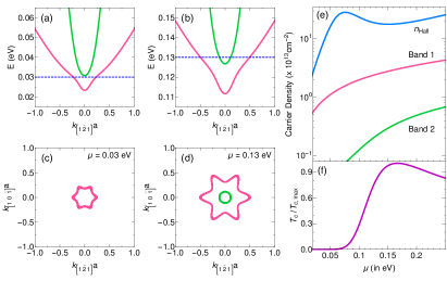
Figure S2: Band structure and transport coefficients at the $(111)$ LaAlO₃/SrTiO₃ interface. Six layers were included in the calculation with a confining potential $V_{\text{c}}=$ 100 meV, while other parameters were identical to those used for Fig. 3 of the main text. The changes in the behavior are insignificant.

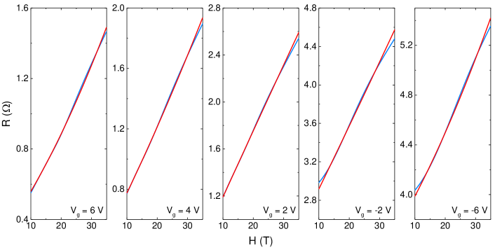
Figure S3: Perpendicular magnetoresistance (blue) at $T=$ 0.34 K for $V_{\text{g}}$ = 6, 4, 2, $-$2, and $-$6 V, together with fits to a quadratic ($a_{0}+a_{\text{1}}H+a_{\text{2}}H^{2}$) function (red).

Clearly, the Hartree-Fock terms renormalize the spin-orbit and crystal-field couplings separately on each layer. To simplify the calculations we further add an overall constant $\epsilon_{\mathcal{I}}$ to the Hamiltonian so that (at $U=0$) the minimum of the lowest band is around zero. For three layers and $t^{\prime\prime}\ll t,V_{c}$, $\epsilon_{\mathcal{I}}$ is

$$\frac{1}{2}\big{(}4t^{\prime\prime}+\Delta_{\text{SO}}-\Delta_{\text{cf}}\big{)}-V_{c}+\sqrt{V_{c}^{2}+2(2t+t^{\prime})^{2}}.$$ (S77)

Transport Coefficients

As explained in the main text, the band structure resulting from the self-consistent calculation of our model is far from isotropic. The six-fold symmetric constant energy surfaces have regions with both positive and negative curvature (Fig. 3(a),(b) of the main text). Therefore in the semi-classical picture, a wave-packet gliding along the Fermi contour (under the effect of a perpendicular magnetic field) would behave as an electron and as a hole at different momenta (different times). The often-employed Drude theory is not valid under these conditions and therefore we use more general expressions, derived from the Boltzmann equation Ong (1991); Hurd (1972), for the longitudinal ($\sigma_{\text{L}}$) and Hall ($\sigma_{\text{H}}$) conductivity,

$$\sigma_{L} =-e^{2}\sum_{m}\int_{BZ}\frac{d^{2}K}{(2\pi)^{2}}\big{(}\partial_{\mu}f[\epsilon_{m}(\vec{K})]\big{)}\tau_{m}(\vec{K})\frac{1}{2}\big{(}\big{[}v^{X}_{m}(\vec{K})\big{]}^{2}+\big{[}v^{Y}_{m}(\vec{K})\big{]}^{2}\big{)},$$ (S78)

$$\sigma_{H} =-e^{3}B\sum_{m}\int_{BZ}\frac{d^{2}K}{(2\pi)^{2}}\big{(}\partial_{\mu}f[\epsilon_{m}(\vec{K})]\big{)}\big{(}v^{X}_{m}(\vec{K})\tau_{m}(\vec{K})\big{)}\big{[}v^{Y}_{m}(\vec{K})\partial_{K_{X}}-v^{X}_{m}(\vec{K})\partial_{K_{Y}}\big{]}\big{(}v^{Y}_{m}(\vec{K})\tau_{m}(\vec{K})\big{)},$$ (S79)

where $m$ runs over the self-consistent bands, $\epsilon_{m}(\vec{K})$ is the energy of the $m$th band at momentum $\vec{K}$, $f[\epsilon_{m}(\vec{K})]$ is the corresponding Fermi-Dirac distribution, $v^{i}_{m}(\vec{K})=\partial_{K_{i}}\epsilon_{m}(\vec{K})$ is the corresponding $i$th component of the group velocity, and $\tau_{m}(\vec{K})$ is the corresponding momentum dependent scattering time. In this work we assume that the momentum dependence of the band lifetimes arises from the momentum-dependent orbital character of the bands. Thus, we define $\tau_{m}$ to be the weighted average of the orbital lifetimes,

$$\tau_{m}(\vec{K})=\sum_{\sigma} \tau_{\text{a}_{\text{1g}}}|\psi_{m}(\text{a}_{\text{1g}},\sigma,\vec{K})|^{2}+$$ (S80)

$$\tau_{\text{e}_{\text{g}}^{\prime}}\big{[}|\psi_{m}(\text{e}_{\text{g}+}^{\prime},\sigma,\vec{K})|^{2}+|\psi_{m}(\text{e}_{\text{g}-}^{\prime},\sigma,\vec{K})|^{2}\big{]}.$$

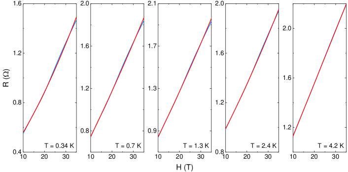
Figure S4: Perpendicular magnetoresistance (blue) at $V_{\text{g}}=$ 6 V for $T=$ 0.34, 0.7, 1.3, 2.4, and 4.2 K, together with fits to a quadratic ($a_{0}+a_{\text{1}}H+a_{\text{2}}H^{2}$) function (red).

This allows $\tau_{m}(k)$ to trace the change in orbital character along the Fermi contour. As discussed in the main text, experimental observations imply that the second band has a larger mobility than the first. Therefore we choose $\tau_{\text{e}_{\text{g}}^{\prime}}>\tau_{\text{a}_{\text{1g}}}$. We note that the orbital lifetimes are assumed to be independent of momentum and energy, which is unlikely to be true in the real material. However, as shown in Fig. 3(e), our results are in agreement with the basic features observed experimentally. Therefore, we believe that the essential physics is correctly captured by our model.

Incorporating Additional Layers

The interface model can be easily extended to include additional layers, since the connectivity of the new atoms is given by the $k_{3}$ dependent terms in $H_{\text{0}}+H_{\text{NNN}}$ [Eqs. (S27)$-$(S32)]. Fig. S2 shows the results of the self-consistent calculation with six layers with the parameters that were used for Fig. 3 of the main text, except for a smaller confining potential, which allows for larger mixing with the deeper layers. Nevertheless, the behavior remains essentially the same as in the three-layer case.

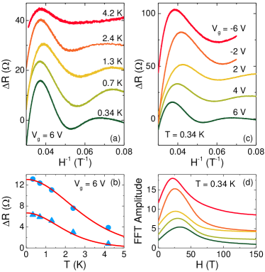
Figure S5: (a) $\Delta R$ as a function of $H^{-1}$ for $T=$ 0.34, 0.7, 1.3, 2.4, and 4.2 K at $V_{\text{g}}=$ 6 V. (b) The temperature dependence of $\Delta R$ at the first maxima and minima in (a). The red lines are the fits to Eq. (S81). (c) $\Delta R$ as a function of $H^{-1}$ for $V_{\text{g}}=$ 6, 4, 2, $-$2, and $-$6 V at $T=$ 0.34 K. (d) The FFT amplitude of $\Delta R$ presented in (c).

S3 III.       Analysis of the Experimental           Magnetotransport Data

We measure the modification of the device resistance ($R$) due to a perpendicular magnetic field ($H$) at $T=$ 340 mK for various $V_{\text{g}}$ (Fig. S3) and at $V_{\text{g}}=$ 6 V for various temperatures (Fig. S4). All the magnetoresistance (MR) measurements show a strong positive MR as reported previously Rout et al. (2017a). In order to extract the Shubnikov-de Haas (SdH) signal, we fit $R$($H$) to a second order polynomial in $H$, $a_{0}+a_{1}H+a_{2}H^{2}$ (See Figs. S3 and S4) and subtract the polynomial background from $R(H)$ to obtain $\Delta R$. The extracted oscillatory resistance $\Delta R$ is plotted in Fig. S5(a) for different temperatures at $V_{\text{g}}=$ 6 V, and in Fig. S5(c) for different $V_{\text{g}}$ at $T=$ 0.34 K. To further analyse $\Delta R$, we use the standard SdH expression Shoenberg (1984),

$${R_{\text{SdH}}}={R_{0}}{e^{-\alpha{T_{\text{D}}}/H}}\frac{{\alpha T/H}}{{\sinh(\alpha T/H)}}\sin(2\pi F/H),$$ (S81)

where $R_{0}$ is a constant pre-factor, $\alpha=2\pi{m^{*}}{k_{B}}/\hbar e$, $m^{*}$ is the cyclotron effective band mass, $T_{\text{D}}$ is the Dingle temperature, and $F$ is the frequency of the oscillation. The best fits to above expression for the oscillation amplitude for the first maxima and minima yield $m^{*}=$ 1.6 $\pm$ 0.1 $m_{\text{e}}$ ($m_{\text{e}}$ being the electron mass) and $T_{\text{D}}=$ 5.4 K corresponding to $V_{\text{g}}=$ 6 V [Fig. S5(b)]. By taking the fast Fourier transform (FFT) of $\Delta R$ for different $V_{\text{g}}$ [Fig. S5(d)], we determine the SdH frequency $F$ as the peak field, which is related to the cross-sectional area $A({\epsilon_{\text{F}}})$ of the 2D Fermi line through the Onsager relation,

$$F=\frac{\hbar}{2\pi e}A({\epsilon_{\text{F}}}).$$ (S82)

Figure S6: (a) The Hall resistance ($R_{\text{xy}}$) as a function of perpendicular magnetic field ($H$) for various $V_{\text{g}}$ at $T=$ 0.34 K. (b) $R_{\text{xy}}$ shifted by 30 $\Omega$ from each other for clarity. The black dashed lines are the linear fit to low field Hall data.

Irrespective of the shape of the Fermi contour, this gives the sheet carrier density of the band which contributes to the SdH oscillations as $n_{\text{SdH}}={N_{\text{v}}}{N_{\text{s}}}eF/h$, where $N_{\text{v}}$ and $N_{\text{s}}$ are the number of valleys and spin species respectively. Fig. 1(a) of the main text presents $n_{\text{SdH}}$ calculated for a single valley and $N_{\text{s}}=2$. Fig. S6 presents the low field Hall measurement performed on the sample at 0.34 K. For all $V_{\text{g}}$ we observe negative Hall slope, which implies the presence of electron-like charge carriers according to standard Drude model. We employed the Drude expressions to determine the Hall carrier density $n_{\text{Hall}}$ [$=(e|R_{\text{H}}|)^{-1}$, where $R_{\text{H}}$ is the Hall coefficient], which is presented in Fig. 1(a) of the main text.

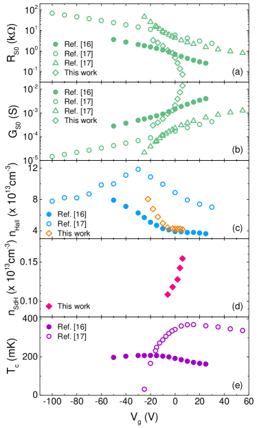
Figure S7: Gate dependence of (a) $R_{\text{S0}}$,(b) $G_{\text{S0}}$,(c) $n_{\text{Hall}}$, (d) $n_{\text{SdH}}$, and (e) $T_{\text{c}}$. We present the new data as well as our previous measurements on $(111)$ LaAlO₃/SrTiO₃ for comparison Rout et al. (2017b); Mograbi et al. (2018). Note that two independent measurements were carried out in Mograbi et al. (2018) to determine $n_{\text{Hall}}$ and $T_{\text{c}}$, which leads to two sets of $R_{\text{S0}}$ and $G_{\text{S0}}$ (as a function of $V_{\text{g}}$).

Figure S7 shows the dependence on gate voltage ($V_{\text{g}}$) of the sheet resistance ($R_{\text{S}}$), sheet conductance ($G_{\text{S0}}=1/R_{\text{S}}$), sheet carrier density determined from low-field Hall measurements ($n_{\text{Hall}}$) and from quantum oscillations ($n_{\text{SdH}}$) as well as the superconducting critical temperature ($T_{\text{c}}$). Fig. 1 of the main text presents $n_{\text{Hall}}$, $n_{\text{SdH}}$, and $T_{\text{c}}$ as a function of $G_{\text{S0}}$.

References

- Bistritzer et al. (2011) R. Bistritzer, G. Khalsa, and A. H. MacDonald, Phys. Rev. B 83, 115114 (2011).
- Khalsa and MacDonald (2012) G. Khalsa and A. H. MacDonald, Phys. Rev. B 86, 125121 (2012).
- Joshua et al. (2012) A. Joshua, S. Pecker, J. Ruhman, E. Altman, and S. Ilani, Nature Communications 3, 1129 (2012).
- Ruhman et al. (2014) J. Ruhman, A. Joshua, S. Ilani, and E. Altman, Phys. Rev. B 90, 125123 (2014).
- Maniv et al. (2015) E. Maniv, M. B. Shalom, A. Ron, M. Mograbi, A. Palevski, M. Goldstein, and Y. Dagan, Nature Communications 6, 8239 (2015).
- Maniv et al. (2017) E. Maniv, Y. Dagan, and M. Goldstein, MRS Advances 2, 1243 (2017).
- Xiao et al. (2011) D. Xiao, W. Zhu, Y. Ran, N. Nagaosa, and S. Okamoto, Nature Communications 2, 596 (2011).
- Okamoto (2013) S. Okamoto, Phys. Rev. Lett. 110, 066403 (2013).
- Okamoto and Xiao (2018) S. Okamoto and D. Xiao, Journal of the Physical Society of Japan 87, 041006 (2018).
- Stamokostas and Fiete (2018) G. L. Stamokostas and G. A. Fiete, Phys. Rev. B 97, 085150 (2018).
- Zhong et al. (2013) Z. Zhong, A. Tóth, and K. Held, Phys. Rev. B 87, 161102 (2013).
- Ong (1991) N. P. Ong, Phys. Rev. B 43, 193 (1991).
- Hurd (1972) C. M. Hurd, The Hall Effect in Metals and Alloys (Plenum Press, New York, 1972).
- Rout et al. (2017a) P. K. Rout, I. Agireen, E. Maniv, M. Goldstein, and Y. Dagan, Phys. Rev. B 95, 241107 (2017a).
- Shoenberg (1984) D. Shoenberg, Magnetic Oscillations in Metals (Cambridge University Press, Cambridge, 1984).
- Rout et al. (2017b) P. K. Rout, E. Maniv, and Y. Dagan, Phys. Rev. Lett. 119, 237002 (2017b).
- Mograbi et al. (2018) M. Mograbi, E. Maniv, P. K. Rout, D. Graf, J.-H. Park, and Y. Dagan, Phys. Rev. B 99, 094507 (2018).