Analysis of random non-autonomous logistic-type differential equations via the Karhunen-Loève expansion and the Random Variable Transformation technique

Abstract

This paper deals with the study, from a probabilistic point of view, of logistic-type differential equations with uncertainties. We assume that the initial condition is a random variable and the diffusion coefficient is a stochastic process. The main objective is to obtain the first probability density function, $f_{1}(p,t)$, of the solution stochastic process, $P(t,\omega)$. To achieve this goal, first the diffusion coefficient is represented via a truncation of order $N$ of the Karhunen-Loève expansion, and second, the Random Variable Transformation technique is applied. In this manner, approximations, say $f_{1}^{N}(p,t)$, of $f_{1}(p,t)$ are constructed. Afterwards, we rigorously prove that $f_{1}^{N}(p,t)\longrightarrow f_{1}(p,t)$ as $N\to\infty$ under mild conditions assumed on input data (initial condition and diffusion coefficient). Finally, three illustrative examples are shown.

1 Motivation and Preliminaries

The prominent role of the logistic differential equation to model problems in different settings as Biology (the dynamics of a population), Economics (the diffusion of a new technology or the growth of an economy), Engineering (the variation of physical properties subject to industrial processes), etc., has been extensively discussed and exhibited in numerous contributions (see for instance [1, 2, 3], [4, 5] and [6, 7], respectively). The logistic differential equation was first proposed by Pierre-François Verhulst, in his celebrated papers [8, 9], to overcome the shortcomings of Malthusian’s model to study the population growth. The main feature of Verhulst’s model versus Malthus’s one is the inclusion of a carrying capacity of the environment, say $M$, which restricts the total number of individuals because resources constrains. Assuming, without loss of generality that $M=1$, the classical logistic model is formulated via the following initial value problem (IVP)

$$\left.\begin{array}[]{lcl}p^{\prime}(t)&=&a(1-p(t))p(t),\\ p(t_{0})&=&p_{0},\end{array}\right\}\quad t>t_{0},\quad 0<p_{0}<1,$$

where $p_{0}$ and $p(t)$ denote the proportions of individuals at the time instants $t_{0}$ and $t>t_{0}$, respectively. This model has been thoroughly studied from different perspectives and using a number of mathematical techniques (see [10, 11], for example). For a fixed initial condition $p_{0}\in]0,1[$, the parameter $a>0$ stands for the reproductive parameter. This parameter depends upon complex variables including environmental factors (weather, food, etc.), genetic factors (birth and death rates, health, etc.), age and other influence factors whose nature is clearly random. Furthermore, the initial condition $p_{0}$ is often calculated via sampling techniques, thus involving randomness, because is not feasible to quantify its value in an exact manner. Hence, it is more realistic to consider that $p_{0}$ is a random variable (RV) rather than a deterministic value. These reasons have motivated the study of logistic-type differential equations with uncertainties both in the initial condition, $p_{0}$, and in the reproductive parameter, $a$. Research on the logistic differential equation with randomness has been conducted using mainly two approaches.

In the first one, uncertainty is introduced via stochastic processes (SPs) whose sample behaviour is very irregular (e.g., nowhere differentiability). This leads to the so-called Stochastic Differential Equations (SDEs). For example, if stochastic perturbations (or noise) are considered by means of a Wiener process like the Brownian motion, then the rigorous treatment of the corresponding SDE requires a special stochastic calculus whose cornerstone result is the Itô lemma [12, 13, 14]. SDEs are formally written via stochastic differentials but rigorously analysed using Riemann-Stieltjes and Itô type stochastic integrals. In this class of SDEs, input noise is limited to Gaussian pattern. Some interesting contributions addressing different formulations of the logistic model or its generalizations, based upon SDEs, include [15, 16, 17, 18].

The second approach consists of direct randomization of input parameters (initial/boundary conditions, forcing terms and/or coefficients) by assigning them suitable probability distributions. This allows to introduce a wider class of stochastic patterns, including the Gaussian one, to describe uncertainties. This leads to the area of Random Differential Equations (RDEs). The so-called Random Mean Square Calculus provides a powerful tool to rigorously tackle RDEs [19, 20]. The study of the logistic RDE, using the Mean Square Calculus and its generalizations, can be found for instance in [21, 22].

Additional approaches based upon SDEs/RDEs formulations to deal with the logistic differential with uncertainty are the moment closure technique [23] and fuzzy variables [24].

In all these contributions dealing with the logistic SDE/RDE, apart from obtaining the solution SP, say $P(t,\omega)$, a major goal is to determine its main statistical functions, namely, the mean function, $\mathbb{E}\left[P(t,\omega)\right]$, and the variance function, $\mathbb{V}\left[P(t,\omega)\right]$. However, a more ambitious target is the computation of its first probability density function (1-PDF), $f_{1}(p,t)$, since via its integration one can compute all the one-dimensional statistical moment functions,

$$\mathbb{E}[\left(P(t,\omega)\right)^{k}]=\int_{-\infty}^{\infty}p^{k}f_{1}(p,t)\,\mathrm{d}p,\quad k=1,2,\ldots,$$ (1)

and, in particular, the mean, $\mathbb{E}\left[P(t,\omega)\right]$, and the variance,

$$\mathbb{V}\left[P(t,\omega)\right]=\mathbb{E}[(P(t,\omega))^{2}]-\mathbb{E}^{2}[P(t,\omega)],$$ (2)

as well as the probability that the population lies in a set of specific interest, say $[p_{1},p_{2}]$,

$$\mathbb{P}\left[p_{1}\leq P(t,\omega)\leq p_{2}\right]=\int_{p_{1}}^{p_{2}}f_{1}(p,t)\,\mathrm{d}p.$$

On the one hand, and to the best of our knowledge, the computation of the 1-PDF of the solution SP of the logistic RDE has been addressed in the two following recent contributions [25, 26], but only in the case that coefficients do not depend on time, i.e., for the so-called random autonomous logistic differential equation. On the other hand, the authors have recently obtained the 1-PDF of the solution SP to the random non-autonomous first-order linear homogeneous differential equation by combing the Karhunen-Loève expansion and the Random Variable Transformation technique [27]. Aimed by this latter result, the goal of this paper is to extend the analysis performed in [27] to the random logistic differential equation assuming that the reproductive parameter is a time-dependent SP, instead of being a RV, and further assuming that the initial condition is a RV. In this manner, here we will deal with the general case from a probabilistic standpoint.

Specifically, we will consider the following random IVP

$$\left.\begin{array}[]{lcl}P^{\prime}(t,\omega)&=&A(t,\omega)(1-P(t,\omega))P(t,\omega),\\ P(t_{0},\omega)&=&P_{0}(\omega),\end{array}\right\}\quad t>t_{0}.$$ (3)

where $A(t,\omega)$ is a SP, $P_{0}(\omega)$ is a bounded absolutely continuous RV $P_{0}:\Omega\longrightarrow[p_{0,1},p_{0,2}]\subset]0,1[$ both satisfying certain hypotheses that will be specified later. These random inputs are defined on a common complete probability space $(\mathbb{P},\mathcal{F},\Omega)$.

Although in the biological setting, the reproductive coefficient in the logistic differential equation is naturally positive, for the sake of generality, in the subsequent analysis we will deal with the general case where $A(t,\omega)$ is not necessarily positive. In this manner, our study will be also valid in more general terms.

Therefore, the main goal of this paper is to compute the 1-PDF of the solution SP of the random IVP (3). To reach this objective, we will combine two important results, namely, the Karhunen-Loève expansion (KLE) and the Random Variable Transformation (RVT) method. The former result will be applied to represent the coefficient $A(t,\omega)$ via an expansion of a denumerable set of zero-mean, unit variance and uncorrelated RVs. By truncating, up to certain order $N$ the KLE of $A(t,\omega)$, we will then apply the RVT method to determine approximations, $f_{1}^{N}(p,t)$ to the exact 1-PDF $f_{1}(p,t)$, for each $(p,t)$ fixed. Afterwards, we will prove the convergence of $f_{1}^{N}(p,t)\longrightarrow f_{1}(p,t)$ as $N\to\infty$ assuming certain hypotheses on input data $P_{0}(\omega)$ and $A(t,\omega)$ that will be specified later on. For the sake of completeness, down below we state both the RVT technique as the KLE.

Theorem 1 (Random Variable Transformation technique)

[19] Let $\mathbf{X}(\omega)=\left(X_{1}(\omega),\ldots,X_{m}(\omega)\right)^{\mathsf{T}}$ and $\mathbf{Y}(\omega)=\left(Y_{1}(\omega),\ldots,Y_{m}(\omega)\right)^{\mathsf{T}}$ be two $m$-dimensional absolutely continuous random vectors defined on a complete probability space $(\Omega,\mathfrak{F},\mathbb{P})$. Let $\mathbf{r}:\mathbb{R}^{m}\rightarrow\mathbb{R}^{m}$ be a one-to-one deterministic transformation of $\mathbf{X}(\omega)$ into $\mathbf{Y}(\omega)$, i.e., $\mathbf{Y}(\omega)=\mathbf{r}(\mathbf{X}(\omega))$, $\omega\in\Omega$. Assume that $\mathbf{r}$ is a continuous mapping and has continuous partial derivatives with respect to each component $x_{i}$, $1\leq i\leq m$. Then, if $f_{\mathbf{x}}(x_{1},\ldots,x_{m})$ denotes the joint probability density function of the vector $\mathbf{X}(\omega)$, and $\mathbf{s}=\mathbf{r}^{-1}=(s_{1}(y_{1},\ldots,y_{m}),\ldots,s_{m}(y_{1},\ldots,y_{m}))$ represents the inverse mapping of $\mathbf{r}=(r_{1}(x_{1},\ldots,x_{m}),\ldots,r_{m}(x_{1},\ldots,x_{m}))$, the joint probability density function of the random vector $\mathbf{Y}(\omega)$ is given by

$$f_{\mathbf{Y}}(y_{1},\ldots,y_{m})=f_{\mathbf{X}}\left(s_{1}(y_{1},\ldots,y_{m}),\ldots,s_{m}(y_{1},\ldots,y_{m})\right)\left|\mathcal{J}_{m}\right|,$$

where $\left|\mathcal{J}_{m}\right|$, which is assumed to be different from zero, denotes the absolute value of the Jacobian defined by the following determinant

$$\mathcal{J}_{m}=\det\left[\begin{array}[]{ccc}\displaystyle\frac{\partial s_{1}(y_{1},\ldots,y_{m})}{\partial y_{1}}&\cdots&\displaystyle\frac{\partial s_{m}(y_{1},\ldots,y_{m})}{\partial y_{1}}\\ \vdots&\ddots&\vdots\\ \displaystyle\frac{\partial s_{1}(y_{1},\ldots,y_{m})}{\partial y_{m}}&\cdots&\displaystyle\frac{\partial s_{m}(y_{1},\ldots,y_{m})}{\partial y_{m}}\\ \end{array}\right]\,.$$

It is worthy highlighting that in the context of RDEs, the RVT technique has been successfully applied to determine the 1-PDF of the solution stochastic process of relevant problems, formulated via RDEs, that appear in different areas [28, 29, 30, 31].

Theorem 2 ($\mathrm{L}^{2}$ convergence of Karhunen-Loève)

[32, p. 202] Consider a mean square integrable continuous time stochastic process $X\equiv\{X(t,\omega):t\in\mathcal{T},\omega\in\Omega\}$, i.e., $X\in\mathrm{L}^{2}(\Omega,\mathrm{L}^{2}(\mathcal{T}))$ being $\mu_{X}(t)$ and $c_{X}(s,t)$ its mean and covariance functions, respectively. Then,

$$X(t,\omega)=\mu_{X}(t)+\sum_{j=1}^{\infty}\sqrt{\nu_{j}}\,\phi_{j}(t)\,\xi_{j}(\omega),\quad\omega\in\Omega,$$ (4)

where, this sum converges in $\mathrm{L}^{2}(\Omega,\mathrm{L}^{2}(\mathcal{T}))$,

$$\xi_{j}(\omega):=\frac{1}{\sqrt{\nu_{j}}}\left<X(t,\omega)-\mu_{X}(t),\phi_{j}(t)\right>_{\mathrm{L}^{2}(\mathcal{T})},$$

$\{(\nu_{j},\phi_{j}(t)):j\geq 1\}$ denote, respectively, the eigenvalues with $\nu_{1}\geq\nu_{2}\geq\cdots\geq 0$ and eigenfunctions of the following integral operator $\mathfrak{C}$

$$(\mathfrak{C}f)(t):=\int_{\mathcal{T}}c_{X}(s,t)f(s)\,\mathrm{d}s,\quad f\in\mathrm{L}^{2}(\mathcal{T}),$$

associated to the covariance function $c_{X}(s,t)$. RVs $\xi_{j}(\omega)$ have zero mean ($\mathbb{E}[\xi_{j}(\omega)]=0$), unit variance ($\mathbb{V}[\xi_{j}(\omega)]=1$) and are pairwise uncorrelated ($\mathbb{E}[\xi_{j}(\omega)\xi_{k}(\omega)]=\delta_{jk}$). Furthermore, if $X(t,\omega)$ is Gaussian, then $\xi_{j}(\omega)\sim\mathrm{N}(0,1)$ are independent and identically distributed.

The space $(\mathrm{L}^{2}(\Omega,\mathrm{L}^{2}(\mathcal{T})),\left\|\cdot\right\|_{\mathrm{L}^{2}(\Omega,\mathrm{L}^{2}(\mathcal{T}))})$ introduced in Th.  2 corresponds to the set of square integrable SPs, $X(t,\omega)$, defined in a set $\mathcal{T}\subset\mathbb{R}$, i.e., $\int_{\mathcal{T}}\mathbb{E}\left[|X(t,\omega)|^{2}\right]\mathrm{d}t<\infty$ (see [32]) with the norm

$$\left\|X(t,\omega)\right\|_{\mathrm{L}^{2}(\Omega,\mathrm{L}^{2}(\mathcal{T}))}=\left(\int_{\mathcal{T}}\mathbb{E}\left[|X(t,\omega)|^{2}\right]\mathrm{d}t\right)^{1/2}<\infty.$$ (5)

We finish this section by stating two results that will be used in the last example of Section 3.

Proposition 1

([33, Th. 8, p. 92]) Let $\{\xi_{i}(\omega):1\leq i\leq N\}$ be independent real random variables defined in a common probability space $(\Omega,\mathcal{F},\mathbb{P})$. Let $f_{i}:\Omega\longrightarrow\mathbb{R}$, $1\leq i\leq N$, be Borel measurable functions. Then, $\{f_{i}(\xi_{i}(\omega)):1\leq i\leq N\}$ are independent random variables.

Proposition 2

([34, p. 21]) Let $\xi(\omega)$ be a random variable defined in a probability space $(\Omega,\mathcal{F},\mathbb{P})$ such that $\mathbb{E}[\xi(\omega)]=0$ and $\mathbb{P}[\{\omega:\alpha\leq\xi(\omega)\leq\beta]=1$. Then,

$$\mathbb{E}\left[\operatorname{e}^{\lambda\xi(\omega)}\right]\leq\operatorname{e}^{\frac{\lambda^{2}(\beta-\alpha)^{2}}{8}},\quad\lambda\in\mathbb{R}.$$

For notational convenience, throughout this paper the exponential function will be written by $\operatorname{e}^{x}$ or $\exp(x)$, interchangeably.

2 Main result: Computing the 1-PDF of the solution stochastic process

This section is firstly addressed to construct approximations, $f_{1}^{N}(p,t)$, of the 1-PDF, $f_{1}(p,t)$, of the solution SP, $P(t,\omega)$, to the random non-autonomous IVP (3), and secondly, to prove that these approximations are convergent, i.e. $f_{1}^{N}(p,t)\longrightarrow f_{1}(p,t)$ as $N\to\infty$, assuming mild conditions on the random inputs $P_{0}(\omega)$ and $A(t,\omega)$.

As the construction of the aforementioned approximation and the proof of its convergence follows a rather technical process, for the sake of clarity we first present an overview of the main ideas that that will be applied to achieve these two goals.

Regarding the construction of the approximation, first we will consider the formal randomization of solution, $P(t,\omega)$, of the logistic model (see below expression (6)), which depends on the stochastic process $A(t)$. Second, we will represent $P(t,\omega)$ in terms of the KLE of $A(t,\omega)$ (see expression (7)). Next, we will truncate this KLE, say $A_{N}(t)$, so that we will obtain a formal approximation, $P_{N}(t,\omega)$, of the solution stochastic process $P(t,\omega)$ (see expression (8)). Then we will apply the RVT method, stated in Th. 1, to obtain the 1-PDF, $f_{1}^{N}(p,t)$, of $P_{N}(t,\omega)$ (see expression (9)). To legitimate this approach, we will assume two hypotheses, that will be denoted by H1 and H2. As we will comment later on, H1 allows us to assure that $P(t,\omega)$ is well defined from a probabilistic standpoint, while H2 guarantees the initial condition, $P_{0}(\omega)$, and the random variables involved in the KLE (see Th. 2), say $(\xi_{1}(\omega),\ldots,\xi_{N}(\omega)):=\boldsymbol{\xi}_{N}(\omega)$, possess respective PDFs. Additionally, all these RVs are assumed to be independent which is a natural assumption in our stochastic setting.

To proof that $f_{1}^{N}(p,t)\longrightarrow f_{1}(p,t)$ as $N\to\infty$, we will apply the classical Cauchy condition assuming two further hypotheses H3 and H4. Hypothesis H3 assumes that the PDF of the initial condition, $f_{P_{0}}(p_{0})$, is Lipschitz. As usual, this assumption permits transferring the behaviour of the increment in the range of $f_{P_{0}}$, that appears when the Cauchy condition is applied, in terms of the information of its domain which involves random variables $P_{0}(\omega)$ and $\xi_{i}(\omega)$, $1\leq i\leq N$. This strategy allows us to take advantage of hypothesis H4 which is related to the growth of the moment-generating function of the KLE of the integral stochastic process $K_{N}(t,\boldsymbol{\xi}_{N}(\omega))\int_{t_{0}}^{t}A_{N}(s,\omega)\,\mathrm{d}s$ (see (10)).

After following the approach previously described, we will summarize our conclusions in a theorem (see Theorem 3).

Hereinafter, we will assume that $t\in\mathcal{T}=[t_{0},T]$, $T>t_{0}$. Motivated by its deterministic counterpart, it is easy to check that a formal solution SP of random IVP (3) is given by

$$P(t,\omega)=\frac{1}{1+\exp{\left(\int_{t_{0}}^{t}-A(s,\omega)\,\mathrm{d}s\right)}\left(-1+\frac{1}{P_{0}(\omega)}\right)},\quad t\in\mathcal{T},\,\,\omega\in\Omega.$$ (6)

We will assume that both random inputs satisfy the following hypothesis:

$$\textbf{H1}:P_{0}:\Omega\longrightarrow[p_{0,1},p_{0,2}]\subset]0,1[\,\,\text{and}\,\,\,A(t,\omega)\in\mathrm{L}^{2}(\Omega,\mathrm{L}^{2}(\mathcal{T})).$$

Remark 1

Notice that the first part of this hypothesis guarantees that the denominator of $P(t,\omega)$ is nonzero with probability 1, thus $P(t,\omega)$ is well-defined almost everywhere (a.e.) regardless the sign of $A(t,\omega)$. Moreover, from (6) it is clear that $P(t,\omega)\neq 0$ a.e. Thus, $P(t,\omega)\in]0,1[$ for all $t\in[t_{0},T]$ and $\omega\in\Omega$ a.e.

On the one hand, notice that as we are assuming the initial condition is bounded, then it is a second-order RV, i.e. $\mathbb{E}[(P_{0}(\omega))^{2}]<+\infty$ (hence having finite variance) and as the time interval $\mathcal{T}$ is closed and bounded, then $P_{0}(\omega)\in\mathrm{L}^{2}(\Omega,\mathrm{L}^{2}(\mathcal{T}))$. On the other hand, since $A(t,\omega)\in\mathrm{L}^{2}(\Omega,\mathrm{L}^{2}(\mathcal{T}))$, it can be represented via the KLE given in (4). Then, the formal solution SP, given in (3), can be written as

$$P(t,\omega)=\displaystyle\frac{1}{1+\exp\left(-\displaystyle\int_{t_{0}}^{t}\left(\mu_{A}(t)+\sum_{j=1}^{\infty}\sqrt{\nu_{j}}\,\phi_{j}(t)\,\xi_{j}(\omega)\right)\,\mathrm{d}s\right)\left(-1+\dfrac{1}{P_{0}(\omega)}\right)},\quad t\in\mathcal{T},\,\,\omega\in\Omega.$$ (7)

Now, we will use this fact together with the RVT technique to construct the approximations $f_{1}^{N}(p,t)$. With this aim, let us consider the truncation of order $N$ of the KLE to $A(t,\omega)$

$$A_{N}(t,\omega)=\mu_{A}(t)+\sum_{j=1}^{N}\sqrt{\nu_{j}}\,\phi_{j}(t)\,\xi_{j}(\omega).$$

Thus, according to (7), the following formal approximation of the truncated solution SP is obtained

$$P_{N}(t,\omega)=\frac{1}{1+\exp\left(\displaystyle-\int_{t_{0}}^{t}\left(\mu_{A}(s)+\sum_{j=1}^{N}\sqrt{\nu_{j}}\,\phi_{j}(s)\,\xi_{j}(\omega)\right)\mathrm{d}s\right)\left(\displaystyle-1+\frac{1}{P_{0}(\omega)}\right)}.$$ (8)

Now, in order to apply the RVT technique, we will assume the following hypothesis

$$\textbf{H2}:\begin{array}[]{cc}P_{0}(\omega),\xi_{i}(\omega),\,\,1\leq i\leq N,\,\,\text{are absolutely continuous RVs.}\\ P_{0}(\omega),\,\,\,\boldsymbol{\xi}_{N}(\omega)=(\xi_{1}(\omega),\dots,\xi_{N}(\omega))\,\,\text{are independent}\\ \text{with PDFs}\,\,f_{P_{0}}(p_{0})\,\,\text{and}\,\,f_{\boldsymbol{\xi}_{N}}(\xi_{1},\dots,\xi_{N}),\,\,\text{respectively}.\end{array}$$

Then, we define the following one-to-one transformation $\mathbf{r}:\mathbb{R}^{N+1}\longrightarrow\mathbb{R}^{N+1}$ componentwise

$$\begin{array}[]{ccccl}y_{1}&=&r_{1}(p_{0},\xi_{1},\dots,\xi_{N})&=&\left(1+\exp\left(\displaystyle-\int_{t_{0}}^{t}\left(\mu_{A}(s)+\sum_{j=1}^{N}\sqrt{\nu_{j}}\,\phi_{j}(s)\,\xi_{j}\right)\mathrm{d}s\right)\left(\displaystyle-1+\frac{1}{p_{0}}\right)\right)^{-1},\\ \\ y_{2}&=&r_{2}(p_{0},\xi_{1},\dots,\xi_{N})&=&\xi_{1},\\ \vdots&&\vdots\\ y_{N+1}&=&r_{N+1}(p_{0},\xi_{1},\dots,\xi_{N})&=&\xi_{N}.\end{array}$$

The inverse of mapping $\mathbf{r}$ is $\mathbf{s}:\mathbb{R}^{N+1}\longrightarrow\mathbb{R}^{N+1}$, whose components are

$$\begin{array}[]{ccccl}p_{0}&=&s_{1}(y_{1},\dots,y_{N+1})&=&\displaystyle\frac{y_{1}\exp\left(\displaystyle-\int_{t_{0}}^{t}\left(\mu_{A}(s)+\sum_{j=1}^{N}\sqrt{\nu_{j}}\,\phi_{j}(s)\,y_{j+1}\right)\mathrm{d}s\right)}{1+y_{1}\left(-1+\exp\left(\displaystyle-\int_{t_{0}}^{t}\left(\mu_{A}(s)+\sum_{j=1}^{N}\sqrt{\nu_{j}}\,\phi_{j}(s)\,y_{j+1}\right)\mathrm{d}s\right)\right)},\\ \\ \xi_{1}&=&s_{2}(y_{1},\dots,y_{N+1})&=&y_{2},\\ \vdots&&\vdots&&\vdots\\ \xi_{N}&=&s_{N+1}(y_{1},\dots,y_{N+1})&=&y_{N+1}.\end{array}$$

Moreover, the absolute value of the Jacobian of the inverse mapping $\mathbf{s}$ is nonzero since

$$\left|J\right|=\left|\frac{\partial s_{1}}{\partial y_{1}}\right|=\frac{\exp\left(\displaystyle-\int_{t_{0}}^{t}\left(\mu_{A}(s)+\sum_{j=1}^{N}\sqrt{\nu_{j}}\,\phi_{j}(s)\,y_{j+1}\right)\mathrm{d}s\right)}{\left(1+y_{1}\left(-1+\exp\left(\displaystyle-\int_{t_{0}}^{t}\left(\mu_{A}(s)+\sum_{j=1}^{N}\sqrt{\nu_{j}}\,\phi_{j}(s)\,y_{j+1}\right)\mathrm{d}s\right)\right)\right)^{2}}\neq 0.$$

Therefore, applying Th. 1, the PDF of the random vector $(Y_{1}(\omega),\dots,Y_{N+1}(\omega))$ is given by

$$\begin{array}[]{lcl}f_{Y_{1},\dots,Y_{N+1}}(y_{1},\dots,y_{N+1})&=&\displaystyle f_{P_{0}}\left(\frac{y_{1}\exp\left(\displaystyle-\int_{t_{0}}^{t}\left(\mu_{A}(s)+\sum_{j=1}^{N}\sqrt{\nu_{j}}\,\phi_{j}(s)\,y_{j+1}\right)\mathrm{d}s\right)}{1+y_{1}\left(-1+\exp\left(\displaystyle-\int_{t_{0}}^{t}\left(\mu_{A}(s)+\sum_{j=1}^{N}\sqrt{\nu_{j}}\,\phi_{j}(s)\,y_{j+1}\right)\mathrm{d}s\right)\right)}\right)\\ \\ &&\times f_{\boldsymbol{\xi}_{N}}\left(y_{2},\dots,y_{N+1}\right)\\ \\ &&\times\displaystyle\frac{\exp\left(\displaystyle-\int_{t_{0}}^{t}\left(\mu_{A}(s)+\sum_{j=1}^{N}\sqrt{\nu_{j}}\,\phi_{j}(s)\,y_{j+1}\right)\mathrm{d}s\right)}{\left(1+y_{1}\left(-1+\exp\left(\displaystyle-\int_{t_{0}}^{t}\left(\mu_{A}(s)+\sum_{j=1}^{N}\sqrt{\nu_{j}}\,\phi_{j}(s)\,y_{j+1}\right)\mathrm{d}s\right)\right)\right)^{2}}.\end{array}$$

Finally, marginalizing with respect to the random vector $(Y_{2}(\omega),\dots,Y_{N+1}(\omega))=\boldsymbol{\xi}_{N}(\omega)$ and taking $t\geq t_{0}$ arbitrary, we obtain the following explicit expression of the 1-PDF of the truncated solution SP, $P_{N}(t,\omega)$,

$$\begin{array}[]{lcl}f_{1}^{N}(p,t)&=&\displaystyle\int_{\mathbb{R}^{N}}f_{P_{0}}\left(\frac{p\exp\left(\displaystyle-\int_{t_{0}}^{t}\left(\mu_{A}(s)+\sum_{j=1}^{N}\sqrt{\nu_{j}}\,\phi_{j}(s)\,\xi_{j}\right)\mathrm{d}s\right)}{1+p\left(-1+\exp\left(\displaystyle-\int_{t_{0}}^{t}\left[\mu_{A}(s)+\sum_{j=1}^{N}\sqrt{\nu_{j}}\,\phi_{j}(s)\,\xi_{j}\right]\mathrm{d}s\right)\right)}\right)\\ \\ &&\times\displaystyle f_{\boldsymbol{\xi}_{N}}\left(\xi_{1},\dots,\xi_{N}\right)\\ \\ &&\times\displaystyle\frac{\exp\left(\displaystyle-\int_{t_{0}}^{t}\left(\mu_{A}(s)+\sum_{j=1}^{N}\sqrt{\nu_{j}}\,\phi_{j}(s)\,\xi_{j}\right)\mathrm{d}s\right)}{\left(1+p\left(-1+\exp\left(\displaystyle-\int_{t_{0}}^{t}\left(\mu_{A}(s)+\sum_{j=1}^{N}\sqrt{\nu_{j}}\,\phi_{j}(s)\,\xi_{j}\right)\mathrm{d}s\right)\right)\right)^{2}}\mathrm{d}\xi_{N}\cdots\mathrm{d}\xi_{1}.\end{array}$$ (9)

In our subsequent analysis, we will provide conditions in order to guarantee the following convergence

$$\lim_{N\to+\infty}f_{1}^{N}(p,t)=f_{1}(p,t),\quad\forall(p,t)\in\mathcal{J}\times[t_{0},T]\,\text{fixed, being}\,\,\mathcal{J}\subset]0,1[\,\,\text{bounded}.$$

Hereinafter, $\hat{p}$ will denote a lower bound of $\mathcal{J}$, i.e., $\hat{p}\in]0,1[$ such that $\hat{p}<p$ for all $p\in\mathcal{J}$. We will prove this convergence by applying the Cauchy condition, i.e., for $\epsilon>0$ fixed, there exist $n_{0}$ (independent of $(p,t)$), such as

$$\left|f_{1}^{N}(p,t)-f_{1}^{M}(p,t)\right|<\epsilon,\quad\forall(p,t)\in\mathcal{J}\times[t_{0},T]\,\text{fixed, being}\,\,\mathcal{J}\subset]0,1[\,\,\text{bounded},\,\,\forall N,M\geq n_{0}.$$

In order to simplify notation, henceforth we will denote

$$K_{N}(t,\boldsymbol{\xi}_{N}(\omega))=\int_{t_{0}}^{t}\left(\mu_{A}(s)+\sum_{j=1}^{N}\sqrt{\nu_{j}}\,\phi_{j}(s)\,\xi_{j}(\omega)\right)\mathrm{d}s.$$ (10)

Thus, expression (9) can be rewritten as

$$f_{1}^{N}(p,t)=\displaystyle\int_{\mathbb{R}^{N}}f_{P_{0}}\left(\frac{p\operatorname{e}^{-K_{N}(t,\boldsymbol{\xi}_{N})}}{1+p\left(-1+\operatorname{e}^{-K_{N}(t,\boldsymbol{\xi}_{N})}\right)}\right)\frac{\operatorname{e}^{-K_{N}(t,\boldsymbol{\xi}_{N})}}{\left(1+p\left(-1+\operatorname{e}^{-K_{N}(t,\boldsymbol{\xi}_{N})}\right)\right)^{2}}f_{\boldsymbol{\xi}_{N}}(\xi_{1},\dots,\xi_{N})\mathrm{d}\xi_{N}\cdots\mathrm{d}\xi_{1}.$$ (11)

Throughout the proof the Steps (I)-(III) will be done. For the sake of clarify, we legitimate these steps later on. Let $(p,t)\in\mathcal{J}\times[t_{0},T]$ fixed, being $\mathcal{J}\subset]0,1[$ bounded, and without loss of generality, take $N>M$. Then,

$$\begin{array}[]{l}\left|f_{1}^{N}(p,t)-f_{1}^{M}(p,t)\right|\\ \\ =\left|\displaystyle\int_{\mathbb{R}^{N}}f_{P_{0}}\left(\frac{p\operatorname{e}^{-K_{N}(t,\boldsymbol{\xi}_{N})}}{1+p\left(-1+\operatorname{e}^{-K_{N}(t,\boldsymbol{\xi}_{N})}\right)}\right)\frac{\operatorname{e}^{-K_{N}(t,\boldsymbol{\xi}_{N})}}{\left(1+p\left(-1+\operatorname{e}^{-K_{N}(t,\boldsymbol{\xi}_{N})}\right)\right)^{2}}f_{\boldsymbol{\xi}_{N}}(\xi_{1},\dots,\xi_{N})\mathrm{d}\xi_{N}\cdots\mathrm{d}\xi_{1}\right.\\ \\ \quad\left.\displaystyle-\int_{\mathbb{R}^{M}}f_{P_{0}}\left(\frac{p\operatorname{e}^{-K_{M}(t,\boldsymbol{\xi}_{M})}}{1+p\left(-1+\operatorname{e}^{-K_{M}(t,\boldsymbol{\xi}_{M})}\right)}\right)\frac{\operatorname{e}^{-K_{M}(t,\boldsymbol{\xi}_{M})}}{\left(1+p\left(-1+\operatorname{e}^{-K_{M}(t,\boldsymbol{\xi}_{M})}\right)\right)^{2}}f_{\boldsymbol{\xi}_{M}}(\xi_{1},\dots,\xi_{M})\mathrm{d}\xi_{M}\cdots\mathrm{d}\xi_{1}\right|\\ \\ \displaystyle\stackrel{{\scriptstyle(\mathrm{I})}}{{=}}\left|\int_{\mathbb{R}^{N}}\left[f_{P_{0}}\left(\frac{p\operatorname{e}^{-K_{N}(t,\boldsymbol{\xi}_{N})}}{1+p\left(-1+\operatorname{e}^{-K_{N}(t,\boldsymbol{\xi}_{N})}\right)}\right)\frac{\operatorname{e}^{-K_{N}(t,\boldsymbol{\xi}_{N})}}{\left(1+p\left(-1+\operatorname{e}^{-K_{N}(t,\boldsymbol{\xi}_{N})}\right)\right)^{2}}\right.\right.\\ \\ \qquad\displaystyle\left.\left.-f_{P_{0}}\left(\frac{p\operatorname{e}^{-K_{M}(t,\boldsymbol{\xi}_{M})}}{1+p\left(-1+\operatorname{e}^{-K_{M}(t,\boldsymbol{\xi}_{M})}\right)}\right)\frac{\operatorname{e}^{-K_{M}(t,\boldsymbol{\xi}_{M})}}{\left(1+p\left(-1+\operatorname{e}^{-K_{M}(t,\boldsymbol{\xi}_{M})}\right)\right)^{2}}\right]f_{\boldsymbol{\xi}_{N}}(\xi_{1},\dots,\xi_{N})\mathrm{d}\xi_{N}\cdots\mathrm{d}\xi_{1}\right|\\ \\ \displaystyle\leq\int_{\mathbb{R}^{N}}\left|\left[f_{P_{0}}\left(\frac{p\operatorname{e}^{-K_{N}(t,\boldsymbol{\xi}_{N})}}{1+p\left(-1+\operatorname{e}^{-K_{N}(t,\boldsymbol{\xi}_{N})}\right)}\right)\frac{\operatorname{e}^{-K_{N}(t,\boldsymbol{\xi}_{N})}}{\left(1+p\left(-1+\operatorname{e}^{-K_{N}(t,\boldsymbol{\xi}_{N})}\right)\right)^{2}}\right.\right.\\ \\ \qquad\displaystyle-f_{P_{0}}\left(\frac{p\operatorname{e}^{-K_{N}(t,\boldsymbol{\xi}_{N})}}{1+p\left(-1+\operatorname{e}^{-K_{N}(t,\boldsymbol{\xi}_{N})}\right)}\right)\frac{\operatorname{e}^{-K_{M}(t,\boldsymbol{\xi}_{M})}}{\left(1+p\left(-1+\operatorname{e}^{-K_{M}(t,\boldsymbol{\xi}_{M})}\right)\right)^{2}}\\ \\ \qquad\displaystyle+f_{P_{0}}\left(\frac{p\operatorname{e}^{-K_{N}(t,\boldsymbol{\xi}_{N})}}{1+p\left(-1+\operatorname{e}^{-K_{N}(t,\boldsymbol{\xi}_{N})}\right)}\right)\frac{\operatorname{e}^{-K_{M}(t,\boldsymbol{\xi}_{M})}}{\left(1+p\left(-1+\operatorname{e}^{-K_{M}(t,\boldsymbol{\xi}_{M})}\right)\right)^{2}}\\ \\ \qquad\displaystyle\left.\left.-f_{P_{0}}\left(\frac{p\operatorname{e}^{-K_{M}(t,\boldsymbol{\xi}_{M})}}{1+p\left(-1+\operatorname{e}^{-K_{M}(t,\boldsymbol{\xi}_{M})}\right)}\right)\frac{\operatorname{e}^{-K_{M}(t,\boldsymbol{\xi}_{M})}}{\left(1+p\left(-1+\operatorname{e}^{-K_{M}(t,\boldsymbol{\xi}_{M})}\right)\right)^{2}}\right]\right|f_{\boldsymbol{\xi}_{N}}(\xi_{1},\dots,\xi_{N})\mathrm{d}\xi_{N}\cdots\mathrm{d}\xi_{1}\\ \\ \displaystyle\leq\int_{\mathbb{R}^{N}}\left[\underbrace{f_{P_{0}}\left(\frac{p\operatorname{e}^{-K_{N}(t,\boldsymbol{\xi}_{N})}}{1+p\left(-1+\operatorname{e}^{-K_{N}(t,\boldsymbol{\xi}_{N})}\right)}\right)}_{(1)}\underbrace{\left|\frac{\operatorname{e}^{-K_{N}(t,\boldsymbol{\xi}_{N})}}{\left(1+p\left(-1+\operatorname{e}^{-K_{N}(t,\boldsymbol{\xi}_{N})}\right)\right)^{2}}-\frac{\operatorname{e}^{-K_{M}(t,\boldsymbol{\xi}_{M})}}{\left(1+p\left(-1+\operatorname{e}^{-K_{M}(t,\boldsymbol{\xi}_{M})}\right)\right)^{2}}\right|}_{(2)}\right.\end{array}$$

$$\begin{array}[]{l}\displaystyle+\left.\underbrace{\left|f_{P_{0}}\left(\frac{p\operatorname{e}^{-K_{N}(t,\boldsymbol{\xi}_{N})}}{1+p\left(-1+\operatorname{e}^{-K_{N}(t,\boldsymbol{\xi}_{N})}\right)}\right)-f_{P_{0}}\left(\frac{p\operatorname{e}^{-K_{M}(t,\boldsymbol{\xi}_{M})}}{1+p\left(-1+\operatorname{e}^{-K_{M}(t,\boldsymbol{\xi}_{M})}\right)}\right)\right|}_{(3)}\underbrace{\frac{\operatorname{e}^{-K_{M}(t,\boldsymbol{\xi}_{M})}}{\left(1+p\left(-1+\operatorname{e}^{-K_{M}(t,\boldsymbol{\xi}_{M})}\right)\right)^{2}}}_{(4)}\right]f_{\boldsymbol{\xi}_{N}}(\xi_{1},\dots,\xi_{N})\mathrm{d}\xi_{N}\cdots\mathrm{d}\xi_{1}\\ \\ \displaystyle\stackrel{{\scriptstyle(\mathrm{II})}}{{<}}\int_{\mathbb{R}^{N}}\left[\left(L_{f_{P_{0}}}(1+p_{0,1})+F_{0}\right)C_{g}|K_{N}(t,\boldsymbol{\xi}_{N})-K_{M}(t,\boldsymbol{\xi}_{M})|\right.\\ \\ \displaystyle\quad\left.+L_{f_{P_{0}}}C_{h}|K_{N}(t,\boldsymbol{\xi}_{N})-K_{M}(t,\boldsymbol{\xi}_{M})|\frac{\operatorname{e}^{K_{M}(t,\boldsymbol{\xi}_{M})}}{\hat{p}^{2}}\right]f_{\boldsymbol{\xi}_{N}}(\xi_{1},\dots,\xi_{N})\mathrm{d}\xi_{N}\dots\mathrm{d}\xi_{1}\\ \\ \displaystyle=\left(L_{f_{P_{0}}}(1+p_{0,1})+F_{0}\right)C_{g}\mathbb{E}\left[|K_{N}(t,\boldsymbol{\xi}_{N}(\omega))-K_{M}(t,\boldsymbol{\xi}_{M}(\omega))|\right]\\ \\ \displaystyle\quad+\frac{L_{f_{P_{0}}}C_{h}}{\hat{p}^{2}}\mathbb{E}\left[|K_{N}(t,\boldsymbol{\xi}_{N}(\omega))-K_{M}(t,\boldsymbol{\xi}_{M}(\omega))|\operatorname{e}^{K_{M}(t,\boldsymbol{\xi}_{M}(\omega))}\right]\\ \\ \displaystyle\leq\left(L_{f_{P_{0}}}(1+p_{0,1})+F_{0}\right)C_{g}\mathbb{E}\left[|K_{N}(t,\boldsymbol{\xi}_{N}(\omega))-K_{M}(t,\boldsymbol{\xi}_{M}(\omega))|^{2}\right]^{1/2}\\ \\ \displaystyle\quad+\frac{L_{f_{P_{0}}}C_{h}}{\hat{p}^{2}}\mathbb{E}\left[|K_{N}(t,\boldsymbol{\xi}_{N}(\omega))-K_{M}(t,\boldsymbol{\xi}_{M}(\omega))|^{2}\right]^{1/2}\mathbb{E}\left[\operatorname{e}^{2K_{M}(t,\boldsymbol{\xi}_{M}(\omega))}\right]^{1/2}\\ \\ \displaystyle=\left(\left(L_{f_{P_{0}}}(1+p_{0,1})+F_{0}\right)C_{g}+\frac{L_{f_{P_{0}}}C_{h}}{\hat{p}^{2}}\mathbb{E}\left[\operatorname{e}^{2K_{M}(t,\boldsymbol{\xi}_{M}(\omega))}\right]^{1/2}\right)\mathbb{E}\left[|K_{N}(t,\boldsymbol{\xi}_{N}(\omega))-K_{M}(t,\boldsymbol{\xi}_{M}(\omega))|^{2}\right]^{1/2}\\ \\ \stackrel{{\scriptstyle(\mathrm{III})}}{{\leq}}\alpha\,\mathbb{E}\left[|K_{N}(t,\boldsymbol{\xi}_{N}(\omega))-K_{M}(t,\boldsymbol{\xi}_{M}(\omega))|^{2}\right]^{1/2}.\end{array}$$

Notice that in the last steps (penultimate equality and inequality), we have applied the definition of the expectation and the Cauchy–Schwarz inequality for expectations, respectively.

Now, we justify the above Steps (I)-(III):
Step (I): As $N>M$, here we have used that the PDF $f_{1}^{M}(p,t)$ can be expressed in terms of PDF $f_{1}^{N}(p,t)$, by marginalizing this latter function with respect to $\xi_{M+1}(\omega),\ldots,\xi_{N}(\omega)$, that is by introducing the corresponding $N-M$-fold integration.
Step (II): The following hypothesis will be assumed to legitimate bounds of this step.

$$\textbf{H3}:\begin{array}[]{c}f_{P_{0}}(p_{0})\,\,\text{is Lipschitz continuous in its domain, i.e.,}\\ \exists\,L_{f_{P_{0}}}>0:\,|f_{P_{0}}(p^{*})-f_{P_{0}}(p^{**})|\leq L_{f_{P_{0}}}|p^{*}-p^{**}|,\quad\forall p^{*},p^{**}\in[p_{0,1},p_{0,2}]\subset]0,1[.\end{array}$$

Using this assumption, we get the bound corresponding to term (1). Let $F_{0}=f_{P_{0}}(p_{0,1})$, by hypothesis H3:

$$\begin{array}[]{lcl}\displaystyle f_{P_{0}}\left(\frac{p\operatorname{e}^{-K_{N}(t,\boldsymbol{\xi}_{N})}}{1+p\left(-1+\operatorname{e}^{-K_{N}(t,\boldsymbol{\xi}_{N})}\right)}\right)&\leq&\displaystyle\left|f_{P_{0}}\left(\frac{p\operatorname{e}^{-K_{N}(t,\boldsymbol{\xi}_{N})}}{1+p\left(-1+\operatorname{e}^{-K_{N}(t,\boldsymbol{\xi}_{N})}\right)}\right)-f_{P_{0}}(p_{0,1})\right|+f_{P_{0}}(p_{0,1})\\ \\ \displaystyle&\leq&\displaystyle L_{f_{P_{0}}}\left|\frac{p\operatorname{e}^{-K_{N}(t,\boldsymbol{\xi}_{N})}}{1+p\left(-1+\operatorname{e}^{-K_{N}(t,\boldsymbol{\xi}_{N})}\right)}-p_{0,1}\right|+F_{0}\\ \\ \displaystyle&\leq&\displaystyle L_{f_{P_{0}}}\left(\left|\frac{p\operatorname{e}^{-K_{N}(t,\boldsymbol{\xi}_{N})}}{1+p\left(-1+\operatorname{e}^{-K_{N}(t,\boldsymbol{\xi}_{N})}\right)}\right|+p_{0,1}\right)+F_{0}\\ \\ &<&\displaystyle L_{f_{P_{0}}}(1+p_{0,1})+F_{0}.\end{array}$$

Observe that in the last inequality we have used Remark 1.

Now, we will bound term (2). With this end the mean value theorem (MVT) will be applied. Let $p\in\mathcal{J}$ be arbitrary but fixed, being $\mathcal{J}\subset]0,1[$ bounded and let us define the auxiliary function

$$g(z)=\frac{\operatorname{e}^{-z}}{(1+p(-1+\operatorname{e}^{-z}))^{2}},\quad z\in\mathbb{R}.$$

Remark 2

We prove that $1+p(-1+\operatorname{e}^{-z})\neq 0$ for all $z\in\mathbb{R}$. Let us reasoning by contradiction. Assume that $1+p(-1+\operatorname{e}^{-z})=0$. The case $z=0$ obviously leads to contradiction. $1+p(-1+\operatorname{e}^{-z})=0$ if and only if $p=\frac{\operatorname{e}^{z}}{\operatorname{e}^{z}-1}$. But, if $z>0$ then $\frac{\operatorname{e}^{z}}{\operatorname{e}^{z}-1}\geq 1$, while if $z<0$ then $\frac{\operatorname{e}^{z}}{\operatorname{e}^{z}-1}<0$. So, both cases lead to contradiction too, since $p\in]0,1[$.

Notice that, by Remark 2 the function $g(z)$ is well-defined. Its derivative $g^{\prime}(z)$ is given by

$$g^{\prime}(z)=-\frac{\operatorname{e}^{z}(\operatorname{e}^{z}(-1+p)+p)}{(\operatorname{e}^{z}(-1+p)-p)^{3}},\quad z\in\mathbb{R}.$$

The function $g^{\prime}(z)$ is bounded for every $p\in\mathcal{J}$, being $\mathcal{J}\subset]0,1[$ bounded:

• By Remark 2 we can assure that $(\operatorname{e}^{z}(-1+p)-p)\neq 0$ (just multiplying $1+p(-1+\operatorname{e}^{-z})\neq 0$ by $-\operatorname{e}^{z}$). Thus $g^{\prime}(z)$ is well-defined for all $z\in\mathbb{R}$.

• Moreover, using L’Hôpital rule, it is easy to check that: $\displaystyle\lim_{z\to\pm\infty}g^{\prime}(z)=0$.

Therefore, $\forall z\in\mathbb{R}$, $\exists C_{g}(p)>0$ such that $|g^{\prime}(z)|\leq C_{g}(p)\leq\sup_{p\in\mathcal{J}}{\{C_{g}(p)\}}=C_{g}$. By applying the MVT there exists $\delta_{g}\in]\min\{K_{N}(t,\boldsymbol{\xi}_{N}),K_{M}(t,\boldsymbol{\xi}_{M})\},\max\{K_{N}(t,\boldsymbol{\xi}_{N}),K_{M}(t,\boldsymbol{\xi}_{M})\}[$ such that

$$\begin{array}[]{lcl}\displaystyle\left|\frac{\operatorname{e}^{-K_{N}(t,\boldsymbol{\xi}_{N})}}{\left(1+p\left(-1+\operatorname{e}^{-K_{N}(t,\boldsymbol{\xi}_{N})}\right)\right)^{2}}-\frac{\operatorname{e}^{-K_{M}(t,\boldsymbol{\xi}_{M})}}{\left(1+p\left(-1+\operatorname{e}^{-K_{M}(t,\boldsymbol{\xi}_{M})}\right)\right)^{2}}\right|&=&|g^{\prime}(\delta_{g})||K_{N}(t,\boldsymbol{\xi}_{N})-K_{M}(t,\boldsymbol{\xi}_{M})|\\ \\ &\leq&C_{g}|K_{N}(t,\boldsymbol{\xi}_{N})-K_{M}(t,\boldsymbol{\xi}_{M})|.\end{array}$$

To bound the expression (3), the same argument exhibited to obtain the bound (2) can be applied. In this case, we apply the MVT to the auxiliary function

$$h(z)=\frac{p\operatorname{e}^{-z}}{1+p(-1+\operatorname{e}^{-z})},\quad z\in\mathbb{R},$$

whose derivative is also bounded, $|h^{\prime}(z)|\leq C_{h}$. Therefore, by Hypothesis H3 and the MVT, it is guaranteed the existence of $\delta_{h}\in]\min\{K_{N}(t,\boldsymbol{\xi}_{N}),K_{M}(t,\boldsymbol{\xi}_{M})\},\max\{K_{N}(t,\boldsymbol{\xi}_{N}),K_{M}(t,\boldsymbol{\xi}_{M})\}[,$ such that

$$\begin{array}[]{l}\displaystyle\left|f_{P_{0}}\left(\frac{p\operatorname{e}^{-K_{N}(t,\boldsymbol{\xi}_{N})}}{1+p\left(-1+\operatorname{e}^{-K_{N}(t,\boldsymbol{\xi}_{N})}\right)}\right)-f_{P_{0}}\left(\frac{p\operatorname{e}^{-K_{M}(t,\boldsymbol{\xi}_{M})}}{1+p\left(-1+\operatorname{e}^{-K_{M}(t,\boldsymbol{\xi}_{M})}\right)}\right)\right|\\ \\ \displaystyle\leq L_{f_{P_{0}}}\left|\frac{p\operatorname{e}^{-K_{N}(t,\boldsymbol{\xi}_{N})}}{1+p\left(-1+\operatorname{e}^{-K_{N}(t,\boldsymbol{\xi}_{N})}\right)}-\frac{p\operatorname{e}^{-K_{M}(t,\boldsymbol{\xi}_{M})}}{1+p\left(-1+\operatorname{e}^{-K_{M}(t,\boldsymbol{\xi}_{M})}\right)}\right|\\ \\ =L_{f_{P_{0}}}|h^{\prime}(\delta_{h})||K_{N}(t,\boldsymbol{\xi}_{N})-K_{M}(t,\boldsymbol{\xi}_{M})|\leq L_{f_{P_{0}}}C_{h}|K_{N}(t,\boldsymbol{\xi}_{N})-K_{M}(t,\boldsymbol{\xi}_{M})|.\end{array}$$

Finally to bound the term (4), as

$$0<\frac{p\operatorname{e}^{-K_{M}(t,\boldsymbol{\xi}_{M})}}{1+p(-1+\operatorname{e}^{-K_{M}(t,\boldsymbol{\xi}_{M})})}<1\quad\text{and}\quad\hat{p}<p,$$

(recall that $\hat{p}<p$ for all $p\in\mathcal{J}$ bounded), then

$$\frac{\operatorname{e}^{-K_{M}(t,\boldsymbol{\xi}_{M})}}{\left(1+p\left(-1+\operatorname{e}^{-K_{M}(t,\boldsymbol{\xi}_{M})}\right)\right)^{2}}=\left(\frac{p\operatorname{e}^{-K_{M}(t,\boldsymbol{\xi}_{M})}}{1+p(-1+\operatorname{e}^{-K_{M}(t,\boldsymbol{\xi}_{M})})}\right)^{2}\frac{\operatorname{e}^{K_{M}(t,\boldsymbol{\xi}_{M})}}{p^{2}}<\frac{\operatorname{e}^{K_{M}(t,\boldsymbol{\xi}_{M})}}{\hat{p}^{2}}.$$

Step (III): In this step of the proof, we assume the following hypothesis

$$\textbf{H4}:\begin{array}[]{c}A(t,\omega)\,\,\text{admits a Karhunen-Lo\`{e}ve expansion of type \eqref{KLEX} such that:}\\ \exists\,C>0:\mathbb{E}\left[\operatorname{e}^{2K_{N}(t,\boldsymbol{\xi}_{N}(\omega))}\right]\leq C,\,\,\text{for all positive integer}\,\,N.\end{array}$$

Then, denoting

$$\alpha=\left(\left(L_{f_{P_{0}}}(1+p_{0,1})+F_{0}\right)C_{g}+\frac{L_{f_{P_{0}}}C_{h}}{\hat{p}^{2}}C^{1/2}\right)>0,$$

the right part of the inequality in the Step (III) is obtained.

Summarizing, under hypotheses H1–H4 we have proved that

$$\left|f_{1}^{N}(p,t)-f_{1}^{M}(p,t)\right|<\alpha\,\mathbb{E}\left[|K_{N}(t,\boldsymbol{\xi}_{N}(\omega))-K_{M}(t,\boldsymbol{\xi}_{M}(\omega))|^{2}\right]^{1/2}.$$

Finally, following the same argument than in [27], that is using Cauchy–Schwarz inequality for integrals, one gets

$$\mathbb{E}\left[\left|K_{N}(t,\boldsymbol{\xi}_{N}(\omega))-K_{M}(t,\boldsymbol{\xi}_{M}(\omega))\right|^{2}\right]\leq(T-t_{0})\left(\left\|A_{N}(t,\omega)-A_{M}(t,\omega)\right\|_{\mathrm{L}^{2}(\Omega,\mathrm{L}^{2}([t_{0},T]))}\right)^{2},$$

and as a consequence of mean square convergence of KLE to $A(t,\omega)$, one obtains

$$\left|f_{1}^{N}(p,t)-f_{1}^{M}(p,t)\right|<\alpha\,\sqrt{T-t_{0}}\left(\left\|A_{N}(t,\omega)-A_{M}(t,\omega)\right\|_{\mathrm{L}^{2}(\Omega,\mathrm{L}^{2}([t_{0},T]))}\right)\xrightarrow[N,M\to+\infty]{}0.$$

Summarizing, the following result has been established:

Theorem 3

Under hypotheses H1–H4, the sequence $\{f^{N}_{1}(p,t):N\geq 1\}$ of 1-PDFs, defined by (11), converges for every $(p,t)\in\mathcal{J}\times[t_{0},T]$, for all $\mathcal{J}\subset\mathbb{R}$ bounded, to the exact 1-PDF, $f_{1}(p,t)$, of the solution SP of random IVP (3).

3 Numerical examples

This section is devoted to illustrate the theoretical findings previously obtained through three numerical examples. In these examples, we will compute approximations to the 1-PDF, $f_{1}(p,t)$, of the solution SP of the random IVP (3) via $f_{1}^{N}(p,t)$, given in (11), for different probability distributions of the initial condition, $P_{0}(\omega)$, and different SPs for the diffusion coefficient, $A(t,\omega)$. In the first example, the standard Wiener process, also termed Browninan motion, will play the role of $A(t,\omega)$, since, in such a case, an exact solution to IVP (3) is available, and then we can check graphic and numerically the accuracy of the approximations, $f_{1}^{N}(p,t)$, for different orders of truncation $N$. Thus, Example 1 is a test example. In the second and third examples, exact solutions are not available. In these two latter cases, we illustrate convergence of approximations of the 1-PDF by means of appropriate graphical representations and also calculating some measure errors that involve two consecutive approximations, namely, $f_{1}^{N}(p,t)$ and $f_{1}^{N-1}(p,t)$. Afterwards, approximations of the mean and variance of the solution SP, $P(t,\omega)$, will be computed in the three examples using the following expressions

$$\mathbb{E}\left[\left(P_{N}(t,\omega)\right)\right]=\int_{-\infty}^{\infty}pf_{1}^{N}(p,t)\,\mathrm{d}p\,,\quad\mathbb{V}\left[\left(P_{N}(t,\omega)\right)\right]=\int_{-\infty}^{\infty}p^{2}f_{1}^{N}(p,t)\,\mathrm{d}p-(\mathbb{E}\left[\left(P_{N}(t,\omega)\right)\right])^{2},$$ (12)

where $P_{N}(t,\omega)$ is defined in (8). Finally, we will assess the accuracy of these approximations (the mean and the variance) via appropriate error measures that will be introduced in the examples.

Example 1

Let us consider the random IVP (3) on the time interval $\mathcal{T}=[t_{0},T]=[0,1.5]$. We choose as initial condition $P_{0}(\omega)$ a Beta RV with parameters $7$ and $10$ truncated on the interval $[0.1,0.9]$, $P_{0}(\omega)\sim\text{Be}_{[0.1,0.9]}(7;10)$ and, as the diffusion coefficient $A(t,\omega)$, the standard Wiener process, $W(t,\omega)$, whose mean and covariance functions are given by $\mu_{W}(t)=0$, $t\in\mathcal{T}$ and $c_{W}(s,t)=\min(s,t)$, $\forall(s,t)\in\mathcal{T}\times\mathcal{T}$, respectively. The KLE of the standard Wiener process is given by (4) with $\xi_{j}(\omega)$ pairwise uncorrelated standard Gaussian RVs, $\xi_{j}(\omega)\sim\text{N}(0;1)$, and being

$$\nu_{j}=\frac{4T^{2}}{(2j-1)^{2}\pi^{2}},\quad\phi_{j}(t)=\sqrt{\frac{2}{T}}\sin\left(\frac{(2j-1)\pi t}{2T}\right),\quad j=1,2,\dots$$

the corresponding eigenvalues and eigenfunctions, respectively, [32, p. 206]. We will choose $P_{0}(\omega)$ so that is independent of the random vector $\boldsymbol{\xi}_{N}=(\xi_{1}(\omega),\ldots,\xi_{N}(\omega))$, for $N$ arbitrary but fixed.

Let us check that hypotheses H1–H4 of Th. 3 hold. Since $P_{0}(\omega)\sim\text{Be}_{[0.1,0.9]}(7;10)$, then first part of hypothesis H1 is clearly satisfied taking $p_{0,1}=0.1$ and $p_{0,2}=0.9$. To check the second part, it is enough to observe that $\int_{t_{0}}^{T}\mathbb{E}[(W(t,\omega))^{2}]\,\mathrm{d}t=\int_{t_{0}}^{T}t\,\mathrm{d}t=\frac{T^{2}}{2}-\frac{t_{0}^{2}}{2}=1.125<\infty$. The hypothesis H2 holds because the choice we have made for initial condition, $P_{0}(\omega)$, and random vector $\boldsymbol{\xi}_{N}(\omega)$. It is straightforward to check that the first derivative of the PDF of $P_{0}(\omega)\sim\text{Be}_{[0.1,0.9]}(7;10)$ is bounded over the domain $[0.1,0.9]$, thus $f_{P_{0}}(p_{0})$ is Lipschitz on $[0.1,0.9]$. This justifies hypothesis H3. Finally, following the same reasoning exhibited in [27, Remark 2], it is checked that hypothesis H4 fulfils.

Thus according to (11), the 1-PDF of the approximate solution SP, $P_{N}(t,\omega)$, is given by

$$f_{1}^{N}(p,t)=\int_{\mathbb{R}^{N}}f_{P_{0}}\left(\frac{p\operatorname{e}^{-\sum_{j=1}^{N}h_{j}(t)\xi_{j}}}{1+p(-1+\operatorname{e}^{-\sum_{j=1}^{N}h_{j}(t)\xi_{j}})}\right)\frac{\prod_{j=1}^{N}f_{\xi_{j}}(\xi_{j})\operatorname{e}^{-h_{j}(t)\xi_{j}}}{\left(1+p\left(-1+\operatorname{e}^{-\sum_{j=1}^{N}h_{j}(t)\xi_{j}}\right)\right)^{2}}\mathrm{d}\xi_{N}\cdots\mathrm{d}\xi_{1},$$ (13)

where $f_{\xi_{j}}(\xi_{j})$ denotes the PDF of $\xi_{j}(\omega)$ for each $j:1\leq j\leq N$ and

$$h_{j}(t)=\left(\frac{2T}{(2j-1)\pi}\right)^{2}\sqrt{\frac{2}{T}}\left(1-\cos\left(\frac{(2j-1)\pi t}{2T}\right)\right).$$ (14)

So far we have obtained the approximations $f_{1}^{N}(p,t)$ to the exact 1-PDF, $f_{1}(p,t)$, of the solution SP of the random IVP (3). Now, we will determine an explicit expression to $f_{1}(p,t)$. To this goal, let us recall that $\int_{0}^{t}W(s,\omega)\mathrm{d}s\sim\text{N}\left(0;\sqrt{\frac{t^{3}}{3}}\right)$, [19, p. 105], hence $\int_{0}^{t}W(s,\omega)\mathrm{d}s\stackrel{{\scriptstyle[}}{{]}}{\text{d}}{=}\sqrt{\frac{t^{3}}{3}}Z(\omega)$, $Z(\omega)\sim\text{N}(0;1)$. Taking into account that the solution SP of the random IVP (3) is expressed in terms of this stochastic integral (see (6) with $A(t,\omega)=W(t)$) and, by applying the RVT technique (see Th. 1), it is straightforwardly to check that

$$f_{1}(p,t)=\int_{\mathbb{R}}f_{P_{0}}\left(\frac{1}{1+\exp\left(\sqrt{\frac{t^{3}}{3}}z\left(-1+\frac{1}{p}\right)\right)}\right)f_{Z}(z)\frac{\exp\left(\sqrt{\frac{t^{3}}{3}}z\right)}{\left(p+\exp\left(\sqrt{\frac{t^{3}}{3}}z\right)(1-p)\right)^{2}}\mathrm{d}z$$ (15)

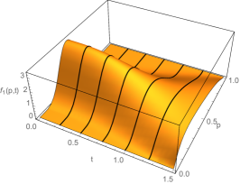
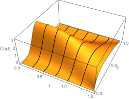
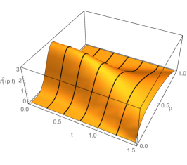
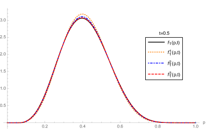
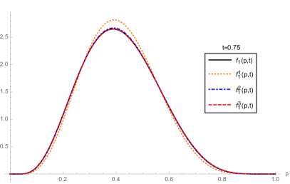
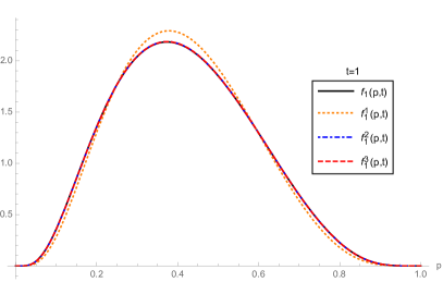
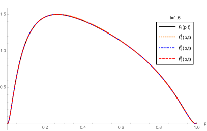
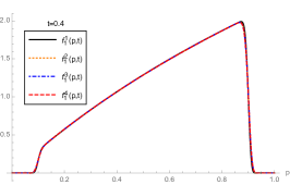
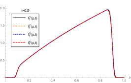
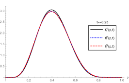
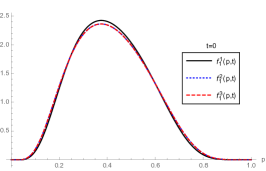
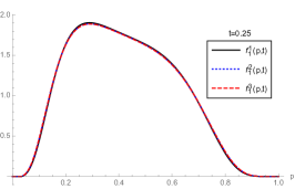
In Figure 1, we show the 1-PDF, $f_{1}(p,t)$, given by (15) of the exact solution SP (7) together with the 1-PDFs, $f_{1}^{N}(p,t)$, given by (13)–(14) corresponding to the approximate solution SP (8) with $N\in\{1,2\}$. We can observe that these approximations $f_{1}^{N}(p,t)$ clearly converge to $f_{1}(p,t)$, even for small values of the order of truncation $N$. For the sake of clarity, in Figure 2 we have plotted the exact 1-PDF, $f_{1}(p,t)$, and the approximate 1-PDFs, $f_{1}^{N}(p,t)$, for $N\in\{1,2,3\}$ at different time instants, $t\in\{0.50,0.75,1.00,1.50\}$. Again, we can observe fast convergence of $f_{1}^{N}(p,t)$ to $f_{1}(p,t)$. In order to better assess this convergence, in Table 1 we have collected the total probabilistic error defined in (16). From these figures we can observe that for $t$ fixed, the error $e_{N}^{\text{PDF}}(t)$ decreases as $N$ increases, as expected.

$$e_{N}^{\text{PDF}}(t)=\int_{0}^{1}\left|f_{1}(p,t)-f_{1}^{N}(p,t)\right|\mathrm{d}p.$$ (16)

Figure 1: Example 1. Left: 1-PDF, $f_{1}(p,t)$, of the exact solution SP given by (15). Center: 1-PDF, $f_{1}^{N}(p,t)$, of the approximate solution given by (13)–(14) with $N=1$. Right: 1-PDF, $f_{1}^{N}(p,t)$, of the approximate solution given by (13)–(14) with $N=2$.

Figure 2: Example 1. Plots of the 1-PDF, $f_{1}(p,t)$, of the exact solution SP given by (15) and the truncations, $f_{1}^{N}(x,t)$, given by (13)–(14) with $N=1,2,3$ for different values of $t$. Left-up: $t=0.50$, Rigth-up: $t=0.75$. Left-down: $t=1.00$. Right-down: $t=1.50$.

$e_{N}^{\text{PDF}}(t)$	$N=1$	$N=2$	$N=3$
$t=0.50$	0.037418	0.013544	0.003149
$t=0.75$	0.059518	0.006964	0.000652
$t=1.00$	0.048595	0.001153	0.000987
$t=1.50$	0.005737	0.000789	0.000648

Table 1: Error measure $e_{N}^{\text{PDF}}(t)$, defined by (16), for different time instants, $t\in\{0.50,0.75,1.00,1.50\}$, and truncation orders $N\in\{1,2,3\}$, in the context of Example 1.

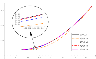
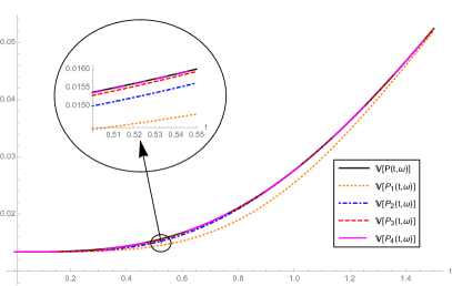
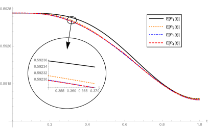
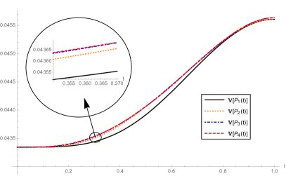
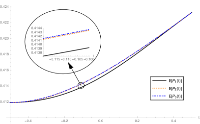
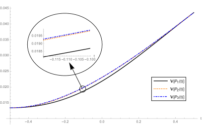
We complete the numerical study by computing the approximations of the mean and the variance functions using (12) and (13)–(14) with $N\in\{1,2,3,4\}$. In Figure 3, we have plotted these approximations together with the exact mean and variance functions obtained via (1), with $k=1,2$, and (2), where $f_{1}(p,t)$ is given by (15). To assess the quality of these approximations, we have computed the total error of the mean and the variance using the following expressions

$$e_{N}^{\mathbb{E}}=\int_{t_{0}}^{T}\left|\mathbb{E}[P(t,\omega)]-\mathbb{E}[P_{N}(t,\omega)]\right|\mathrm{d}t,\qquad e_{N}^{\mathbb{V}}=\int_{t_{0}}^{T}\left|\mathbb{V}[P(t,\omega)]-\mathbb{V}[P_{N}(t,\omega)]\right|\mathrm{d}t.$$ (17)

In Table 2, we show the values of errors $e_{N}^{\mathbb{E}}$ and $e_{N}^{\mathbb{V}}$ for $N\in\{1,2,3,4\}$. From these figures we can observe that both errors decreases as $N$ increases, thus showing fully agreement with the graphical representation shown in Figure 3.

Figure 3: Example 1. Left: Exact mean, $\mathbb{E}[P(t,\omega)]$, of the solution SP and its approximations using truncations of order $N\in\{1,2,3,4\}$ ($\mathbb{E}[P_{i}(t,\omega)]$, $i=1,2,3,4$). Right: Exact variance ($\mathbb{V}[P(t,\omega)]$) of the solution and its approximations using truncations of order $N\in\{1,2,3,4\}$ ($\mathbb{V}[P_{i}(t,\omega)]$, $i=1,2,3,4$).

Error	$N=1$	$N=2$	$N=3$	$N=4$
Mean $e_{N}^{\mathbb{E}}$	0.000659	0.000085	0.000029	0.000009
Variance $e_{N}^{\mathbb{V}}$	0.001756	0.000225	0.000077	0.000035

Table 2: Values of errors $e_{N}^{\mathbb{E}}$ and $e_{N}^{\mathbb{V}}$ for the mean and variance, respectively, given by (17) using different orders of truncation $N\in\{1,2,3,4\}$, in the context of Example 1.

Example 2

Now we will consider the random IVP (3) on the time interval $\mathcal{T}=[t_{0},T]=[0,1]$. We assume that the initial condition $P_{0}(\omega)$ has a truncated Exponential distribution on the interval $[0.1,0.9]$ and with parameter $\lambda=10$, i.e. $P_{0}(\omega)\sim\text{Exp}_{[0.1,0.9]}(10)$. For the diffusion coefficient, $A(t,\omega)$, we will choose the Brownian Bridge [32, p. 193–195]. This SP, say $X(t,\omega)$, is defined in terms of the Wiener SP as $X(t,\omega)=W(t,\omega)-tW(1,\omega)$, having zero-mean, $\mu_{X}(t)=0$, and correlation function

$$c_{X}(s,t)=\min(s,t)-st,\quad(s,t)\in\mathcal{T}\times\mathcal{T}.$$

In [32, p. 204], it is shown that the KLE of the Brownian Bridge is given by (4) being $\xi_{j}(\omega)\sim\text{N}(0,1)$ pairwise uncorrelated RVs and

$$\nu_{j}=\frac{1}{\pi^{2}j^{2}},\quad\phi_{j}(t)=\sqrt{2}\sin(j\pi t),\quad t\in\mathcal{T},j=1,2,\ldots.$$

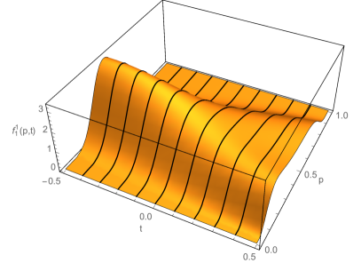
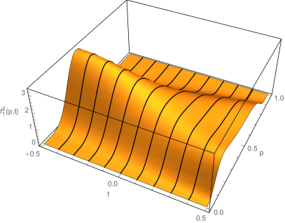
We will choose the random initial condition, $P_{0}(\omega)$, so that is independent of the random vector $\boldsymbol{\xi}_{N}(\omega)=(\xi_{1}(\omega),\ldots,\xi_{N}(\omega))$, for $N$ arbitrary but fixed. Analogously to Example 1, it can be checked that hypotheses H1–H4 fulfil. Therefore, according to (11), the 1-PDF of the approximate solution SP, $P_{N}(t,\omega)$, is given by

$$f_{1}^{N}(p,t)=\int_{\mathbb{R}^{N}}f_{P_{0}}\left(\frac{p\prod_{j=1}^{N}\operatorname{e}^{-h^{*}_{j}(t)\xi_{j}}}{1+p\left(-1+\prod_{j=1}^{N}\operatorname{e}^{-h^{*}_{j}(t)\xi_{j}}\right)}\right)\frac{\prod_{j=1}^{N}\operatorname{e}^{-h^{*}_{j}(t)\xi_{j}}f_{\xi_{j}}(\xi_{j})}{\left(1+p\left(-1+\prod_{j=1}^{N}\operatorname{e}^{-h^{*}_{j}(t)\xi_{j}}\right)\right)^{2}}\mathrm{d}\xi_{N}\dots\mathrm{d}\xi_{1},$$ (18)

where

$$h^{*}_{j}(t)=\frac{\sqrt{2}}{(\pi j)^{2}}(1-\cos(j\pi t)).$$ (19)

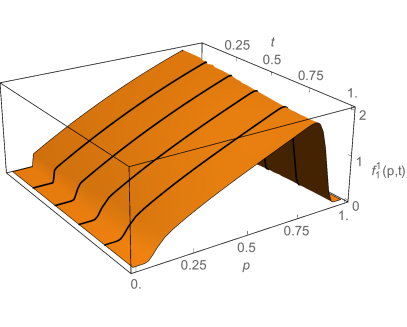
In Figure 4, we show the surface corresponding to the 1-PDF, $f_{1}^{N}(p,t)$, given in (18)–(19) for $N=1$ and $N=2$. We can observe that both approximations are very similar, then showing convergence. For the sake of clarity, in Figure 5, we have represented the 1-PDF, $f_{1}^{N}(p,t)$, at different fixed time instants $t\in\{0.25,0.40,0.50\}$, and increasing the order of truncation $N\in\{1,2,3,4\}$. From these graphical representations, we clearly observe fast convergence on the whole domain. To illustrate numerically this convergence, in Table 3 we show the total difference between two consecutive approximations, $f_{1}^{N}(p,t)$ and $f_{1}^{N-1}(p,t)$, at the time instants previously indicated, using the following error formula

$$\hat{e}_{N}^{PDF}(t)=\int_{0}^{1}\left|f_{1}^{N}(p,t)-f_{1}^{N-1}(p,t)\right|\mathrm{d}p,\quad N=2,3,\ldots.$$ (20)

From figures in Table 3 we can observe that for $t$ fixed, the error $\hat{e}_{N}^{PDF}(t)$ decreases as $N$ increases.

Figure 4: Example 2. Surfaces of the 1-PDF, $f_{1}^{N}(p,t)$, given in (18)–(19) for $N=1$ (Left) and $N=2$ (Right).

Figure 5: Example 2. Curves of the 1-PDF, $f_{1}^{N}(p,t)$, given in (18)–(19) at three different time instants $t=0.25$ (Left), $t=0.40$ (Center) and $t=0.50$ (Right) using, in each case, different orders of truncations $N\in\{1,2,3,4\}$.

$\hat{e}_{N}^{\text{PDF}}(t)$	$N=2$	$N=3$	$N=4$
$t=0.25$	0.002382	0.001275	0.000604
$t=0.40$	0.004166	0.000746	0.000252
$t=0.50$	0.003935	0.000471	0.000306

Table 3: Error measure $\hat{e}_{N}^{\text{PDF}}(t)$ defined by (20) at different time instants, $t\in\{0.25,0.40,0.50\}$, and different orders of truncation $N\in\{2,3,4\}$, in the context of Example 2.

Finally, we take advantage of the approximations, $f_{1}^{N}(p,t)$, of the 1-PDF of the solution SP to compute approximations of the mean, $\mathbb{E}[P_{N}(t,\omega)]$, and the variance, $\mathbb{V}[P_{N}(t,\omega)]$, for different orders of truncation $N\in\{1,2,3,4\}$. These approximations have been plotted in Figure 6. In Table 4, we show the values of the following error measure between consecutive approximations of the mean and the variance on the whole time interval.

$$\hat{e}_{N}^{\mathbb{E}}=\int_{0}^{1}\left|\mathbb{E}[P_{N}(t,\omega)]-\mathbb{E}[P_{N-1}(t,\omega)]\right|\mathrm{d}t,\qquad\hat{e}_{N}^{\mathbb{V}}=\int_{0}^{1}\left|\mathbb{V}[P_{N}(t,\omega)]-\mathbb{V}[P_{N-1}(t,\omega)]\right|\mathrm{d}t.$$ (21)

Figure 6: Example 2. Left: Approximations of the mean, $\mathbb{E}[P_{N}(t,\omega)]$. Right: Approximations of the variance, $\mathbb{V}[P_{N}(t,\omega)]$. In both cases we have taken the following orders of truncations $N\in\{1,2,3,4\}$.

Error	$N=2$	$N=3$	$N=4$
Mean $\hat{e}_{N}^{\mathbb{E}}$	0.000027	0.000005	0.000002
Variance $\hat{e}_{N}^{\mathbb{V}}$	0.000053	0.000011	0.000004

Table 4: Values of errors $\hat{e}_{N}^{\mathbb{E}}$ and $\hat{e}_{N}^{\mathbb{V}}$ for the mean and variance, respectively, given by (21) using different orders of truncation $N\in\{2,3,4\}$, in the context of Example 2.

Example 3

We complete the numerical experiments considering the random IVP (3) on the time interval $\mathcal{T}=[t_{0},T]=[-a,a]$, with $a=0.5$. We assume that the initial condition $P_{0}(\omega)$ has a Beta distribution truncated to the interval $[0.1,0.9]$ and parameters $\alpha=7$ and $\beta=10$, i.e. $P_{0}(\omega)\sim\text{Be}_{[0.1,0.9]}(7;10)$. Regarding the diffusion coefficient, $A(t,\omega)$, and in order to apply our theoretical results, we only need to fix the information involved in its KLE (4), i.e., a family of zero-mean, unit variance and pairwise uncorrelated RVs, $\xi_{j}(\omega)$, the mean function, $\mu_{A}(t)$, and the covariance function, $c_{A}(s,t)$. Now we will choose:

• $\xi_{j}(\omega)$ independent and identically distributed uniform RVs, $\xi_{j}(\omega)\sim\text{Un}(-\sqrt{3},\sqrt{3})$. Thus, $\mathbb{E}[\xi_{j}(\omega)]=0$, $\mathbb{V}[\xi_{j}(\omega)]=1$ and $\mathbb{E}[\xi_{j}(\omega)\xi_{k}(\omega)]=0$, if $j\neq k$.

• Mean function: $\mu_{A}(t)=0$.

• Covariance function

  $$c_{A}(s,t)=\operatorname{e}^{-c|s-t|},\quad(s,t)\in\mathcal{T}\times\mathcal{T},$$

  where $c=1/b>0$, being $b>0$ the so-called correlation length.

According to [35, pp. 26–29], the eigenvalues $\nu_{j}$ and eigenfunctions $\phi_{j}$ of the covariance function $c_{A}(s,t)$ are given by

$$\begin{array}[]{ll}\displaystyle\nu_{j}=\frac{2c}{w_{j}^{2}+c^{2}},&\displaystyle\phi_{j}(t)=\frac{\cos(w_{j}t)}{\sqrt{a+\frac{\sin(2w_{j}a)}{2w_{j}}}},\quad j\text{ odd},\\ \\ \displaystyle\nu_{j}^{*}=\frac{2c}{\left(w_{j}^{*}\right)^{2}+c^{2}},&\displaystyle\phi_{j}^{*}(t)=\frac{\sin(w_{j}^{*}t)}{\sqrt{a-\frac{\sin(2w_{j}^{*}a)}{2w_{j}^{*}}}},\quad j\text{ even},\end{array}$$ (22)

where $w_{j}$, $w_{j}^{*}$ are the solutions of the following transcendental equations

$$\begin{array}[]{l}c-w_{j}\tan(w_{j}a)=0,\quad j\text{ odd},\\ \\ w_{j}^{*}+c\tan(w_{j}^{*}a)=0,\quad j\text{ even}.\end{array}$$

Therefore the diffusion SP, $A(t,\omega)$, is represented by the following KLE

$$A(t,\omega)=\sum_{j=1}^{\infty}\left(\sqrt{\nu_{2j-1}}\phi_{2j-1}(t)\xi_{2j-1}(\omega)+\sqrt{\nu_{2j}^{*}}\phi_{2j}^{*}(t)\xi_{2j}^{*}(\omega)\right).$$ (23)

In order to guarantee that hypothesis H2 fulfils, as in the two previous examples we will choose the initial condition $P_{0}(\omega)$ so that is independent of the random vector $\boldsymbol{\xi}_{N}(\omega)=(\xi_{1}(\omega),\ldots,\xi_{N}(\omega))$, for $N$ arbitrary, but fixed. Now we check that hypotheses H1, H3 and H4 hold. First part of hypothesis H1 is evident while the second part follows because $\int_{-a}^{a}\mathbb{E}[(A(t,\omega))^{2}]\,\mathrm{d}t=\int_{-a}^{a}c_{A}(t,t)\,\mathrm{d}t=\int_{-a}^{a}1\,\mathrm{d}t=2a<\infty$. Hypothesis H3 can be checked in a similar way as in Example 1. To verify that the hypothesis H4 holds, we will follow a similar reasoning to the one exhibited in [27, Remark 2], but now taking advantage of Prop. 2. First, let us observe that using (10) and the independence of $\xi_{1}(\omega),\ldots,\xi_{N}(\omega)$, for each $t\in[-a,a]$ and Prop. 1, one gets,

$$\begin{array}[]{ccl}\mathbb{E}[\operatorname{e}^{2K_{N}(t,\boldsymbol{\xi}(\omega))}]&=&\displaystyle\mathbb{E}\left[\exp\left(2\int_{-a}^{t}\left(\sum_{j=1}^{N}\left(\sqrt{\nu_{2j-1}}\,\phi_{2j-1}(s)\,\xi_{2j-1}(\omega)+\sqrt{\nu_{2j}^{\ast}}\,\phi_{2j}^{\ast}(s)\,\xi_{2j}^{\ast}(\omega)\right)\right)\mathrm{d}s\right)\right]\\ \\ &=&\displaystyle\prod_{j=1}^{N}\mathbb{E}\left[\exp\left(\lambda_{2j-1}(t)\,\xi_{2j-1}(\omega)\right)\right]\mathbb{E}\left[\exp\left(\lambda_{2j}^{\ast}(t)\,\xi_{2j}^{\ast}(\omega)\right)\right],\end{array}$$ (24)

where

$$\lambda_{2j-1}(t)=2\sqrt{\nu_{2j-1}}\int_{-a}^{t}\phi_{2j-1}(s)\,\mathrm{d}s,\quad\lambda_{2j}^{\ast}(t)=2\sqrt{\nu_{2j}^{\ast}}\int_{-a}^{t}\phi_{2j}^{\ast}(s)\,\mathrm{d}s.$$

Now, we apply Prop. 2 to each one of the expectations that appear in the last product in (24) (for the first factor we take $\lambda=\lambda_{2j-1}(t)$ and $\xi(\omega)=\xi_{2j-1}(\omega)$, for the second one, $\lambda=\lambda_{2j}^{\ast}(t)$ and $\xi(\omega)=\xi_{2j}^{\ast}(\omega)$, and $\alpha=-\sqrt{3}$ and $\beta=\sqrt{3}$). This yields

$$\begin{array}[]{ccl}\mathbb{E}[\operatorname{e}^{2K_{N}(t;\boldsymbol{\xi}(\omega))}]&\leq&\displaystyle\prod_{j=1}^{N}\exp\left(6\nu_{2j-1}\left(\int_{-a}^{t}\phi_{2j-1}(s)\,\mathrm{d}s\right)^{2}\right)\exp\left(6\nu_{2j}^{\ast}\left(\int_{-a}^{t}\phi_{2j}^{\ast}(s)\,\mathrm{d}s\right)^{2}\right)\\ \\ &=&\exp\left(\displaystyle 6\sum_{j=1}^{N}\left(\nu_{2j-1}\left(\int_{-a}^{t}\phi_{2j-1}(s)\,\mathrm{d}s\right)^{2}+\nu_{2j}^{\ast}\left(\int_{-a}^{t}\phi_{2j}^{\ast}(s)\,\mathrm{d}s\right)^{2}\right)\right)\end{array}$$ (25)

Now, we will apply the Cauchy-Schwarz inequality for integrals and the fact that $t\in[-a,a]$, then

$$\left(\int_{-a}^{t}\phi_{2j-1}(s)\,\mathrm{d}s\right)^{2}\leq(t+a)\int_{-a}^{t}\left(\phi_{2j-1}(s)\right)^{2}\mathrm{d}s\leq 2a\int_{-a}^{a}\left(\phi_{2j-1}(s)\right)^{2}\mathrm{d}s,$$

and analogously,

$$\left(\int_{-a}^{t}\phi_{2j}^{\ast}(s)\,\mathrm{d}s\right)^{2}\leq 2a\int_{-a}^{a}\left(\phi_{2j}^{\ast}(s)\right)^{2}\mathrm{d}s.$$

As a consequence, the inequality (25) becomes

$$\begin{array}[]{ccl}\mathbb{E}[\operatorname{e}^{2K_{N}(t;\boldsymbol{\xi}(\omega))}]&\leq&\exp\left(\displaystyle 12a\sum_{j=1}^{N}\left(\nu_{2j-1}\int_{-a}^{a}\left(\phi_{2j-1}(s)\right)^{2}\mathrm{d}s+\nu_{2j}^{\ast}\int_{-a}^{a}\left(\phi_{2j}^{\ast}(s)\right)^{2}\mathrm{d}s\right)\right)\\ \\ &=&\exp\left(\displaystyle 12a\left(\int_{-a}^{a}\sum_{j=1}^{N}\nu_{2j-1}\left(\phi_{2j-1}(s)\right)^{2}\mathrm{d}s+\int_{-a}^{a}\sum_{j=1}^{N}\nu_{2j}^{\ast}\left(\phi_{2j}^{\ast}(s)\right)^{2}\mathrm{d}s\right)\right)\\ \\ &\leq&\exp\left(\displaystyle 12a\int_{-a}^{a}\left(\sum_{j=1}^{\infty}\nu_{2j-1}\left(\phi_{2j-1}(s)\right)^{2}+\nu_{2j}^{\ast}\left(\phi_{2j}^{\ast}(s)\right)^{2}\right)\mathrm{d}s\right),\end{array}$$ (26)

where in the last step we have applied that $\nu_{2j-1}>0$ and $\nu_{2j}^{\ast}>0$ for every $j\geq 1$ (see (22)).

On the other hand, if we square the expression of $A(t;\omega)$ given in (23) and afterwards we take the expectation operator and use that $\mathbb{E}[\xi_{2j-1}(\omega)]=\mathbb{E}[\xi_{2j}^{\ast}(\omega)]=0$, $\mathbb{V}[\xi_{2j-1}(\omega)]=\mathbb{V}[\xi_{2j}^{\ast}(\omega)]=1$ and $\mathbb{E}[\xi_{j}(\omega)\xi_{k}(\omega)]=0$ if $j\neq k$, one obtains

$$\mathbb{E}[(A(t;\omega))^{2}]=\sum_{j=1}^{\infty}\left(\nu_{2j-1}\left(\phi_{2j-1}(t)\right)^{2}+\nu_{2j}^{\ast}\left(\phi_{2j}^{\ast}(t)\right)^{2}\right).$$

Integrating both sides and taking into account that $A(t,\omega)\in\mathrm{L}^{2}(\Omega,\mathrm{L}^{2}(\mathcal{T}))$, $\mathcal{T}=[-a,a]$ and using the norm defined in (5), one gets

$$\int_{-a}^{a}\sum_{j=1}^{\infty}\left(\nu_{2j-1}\left(\phi_{2j-1}(t)\right)^{2}+\nu_{2j}^{\ast}\left(\phi_{2j}^{\ast}(t)\right)^{2}\right)\,\mathrm{d}t=\int_{-a}^{a}\mathbb{E}[(A(t;\omega))^{2}]\,\mathrm{d}t=\left(\left\|A(t,\omega)\right\|_{\mathrm{L}^{2}(\Omega,\mathrm{L}^{2}([-a,a]))}\right)^{2}<\infty.$$

As a consequence, using this last conclusion in expression (26), one derives that $\mathbb{E}[\operatorname{e}^{2K_{N}(t;\boldsymbol{\xi}(\omega))}]<\infty$ for every $t\in[-a,a]$ and for all $N\geq 1$ positive integer. Therefore, the hypothesis H4 fulfils.

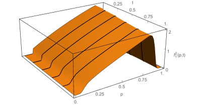
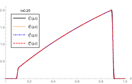
Now, we do not show the explicit algebraic expression of the approximations, $f_{1}^{N}(p,t)$, because it is somewhat cumbersome, but is clear that it could be calculated in the same manner we did in the two previous examples. In Figure 7, we show the surfaces corresponding to those approximations for $N=1$ and $N=2$. From these two plots, we can observe that both surfaces are very similar, then showing a fast convergence. In Figure 8, we show the approximations $f_{1}^{N}(p,t)$ at different time instants $t\in\{-0.25,0,0.25\}$ and using different orders of truncations $N\in\{1,2,3\}$. Again, we observe fast convergence in all these cases. We use an analogous measure to the one defined in (20), i.e.,

$$\hat{e}_{N}^{PDF}(t)=\int_{-0.5}^{0.5}\left|f_{1}^{N}(p,t)-f_{1}^{N-1}(p,t)\right|\mathrm{d}p,\quad N=2,3,\ldots,$$ (27)

to illustrate this convergence. In Table 5, we have collected figures of $\hat{e}_{N}^{\text{PDF}}(t)$ for the values of $t$ and $N$ previously indicated.

Figure 7: Example 3. Surfaces of the 1-PDF, $f_{1}^{N}(p,t)$, for $N=1$ (Left) and $N=2$ (Right).

Figure 8: Example 3. Curves of the 1-PDF, $f_{1}^{N}(p,t)$ at three different times $t=-0.25$ (Left), $t=0$ (Center) and $t=0.25$ (Right) using, in each case, different orders of truncations $N\in\{1,2,3\}$.

$\hat{e}_{N}^{\text{PDF}}(t)$	$N=2$	$N=3$
$t=-0.25$	0.022077	0.004105
$t=0$	0.029739	0.000044
$t=0.25$	0.009479	0.000975

Table 5: Error measure $\hat{e}_{N}^{\text{PDF}}(t)$ defined by (27) for different time instants, $t\in\{-0.25,0,0.25\}$, and truncation orders $N\in\{2,3\}$, in the context of Example 3.

We finally compute approximations of the mean, $\mathbb{E}[P_{N}(t,\omega)]$, and the variance, $\mathbb{V}[P_{N}(t,\omega)]$, for $N\in\{1,2,3,4\}$. These approximations have been represented in Figure 9. From these graphical representations we evince fast convergence of both statistical moments. In Table 6, we illustrate numerically this convergence by computing the total difference between consecutive approximations of the mean and variance on the whole time interval via the expressions given in (28).

$$\hat{e}_{N}^{\mathbb{E}}=\int_{-0.5}^{0.5}\left|\mathbb{E}[P_{N}(t,\omega)]-\mathbb{E}[P_{N-1}(t,\omega)]\right|\mathrm{d}t,\qquad\hat{e}_{N}^{\mathbb{V}}=\int_{-0.5}^{0.5}\left|\mathbb{V}[P_{N}(t,\omega)]-\mathbb{V}[P_{N-1}(t,\omega)]\right|\mathrm{d}t.$$ (28)

Figure 9: Example 3. Left: Approximations of the mean, $\mathbb{E}[P_{N}(t,\omega)]$. Right: Approximations of the variance, $\mathbb{V}[P_{N}(t,\omega)]$. In both cases we have taken the following orders of truncations $N\in\{1,2,3\}$.

Error	$N=2$	$N=3$
Mean $\hat{e}_{N}^{\mathbb{E}}$	0.000216	0.000016
Variance $\hat{e}_{N}^{\mathbb{V}}$	0.000575	0.000042

Table 6: Values of errors $\hat{e}_{N}^{\mathbb{E}}$ and $\hat{e}_{N}^{\mathbb{V}}$ for the mean and variance, respectively, given by (28) using different orders of truncation $N\in\{2,3\}$, in the context of Example 3.

4 Conclusions

In this paper we have studied a generalization of the random logistic differential equation consisting of assuming that the diffusion coefficient is a stochastic process and with a random initial condition. Under general hypotheses on random data, we have constructed approximations of the first probability density function of the solution stochastic process. The key tools for conducting our analysis have been the Random Variable Transformation method together with the Karhunen-Loève expansions. Our theoretical findings have been illustrated by means of several examples. To the best of our knowledge, it is first time that our approach is applied to a random non-autonomous nonlinear differential equation. We think that this contribution can be useful to study other important random nonlinear differential equations.

Conflict of Interest Statement

The authors declare that there is no conflict of interests regarding the publication of this article.

References

- [1] F. Guidi, L. Pezzolesi, S. Vanucci, Microbial dynamics during harmful dinoflagellate Ostreopsis cf. ovata growth: Bacterial succession and viral abundance pattern, Microbiology Open (2018) 1–15. doi:10.1002/mbo3.584.
- [2] L. Fu, Z. Wei, K. Hu, L. Hu, Y. Li, X. Chen, G. Yao, H. Zhang, Hydrogen sulfide inhibits the growth of Escherichia coli through oxidative damage, Journal of Microbiology (2018) 1–8. doi:10.1007/s12275-018-7537-1.
- [3] A. Fredrik, N. Andreas, N. Jan-Ake, Experimentally increased nest temperature affects body temperature, growth and apparent survival in blue tit nestlings, Journal of Avian Biology 49 (2) (2018) 1–14. doi:10.1111/jav.01620.
- [4] S. Shumska, Growth prospects of Ukrainian economy against the background of global trends, Economy and Forecasting 2017 (3) (2017) 7–30. doi:10.15407/eip2017.03.007.
- [5] A. Lotfi, A. Lotfi, K. Hu, W. E. Halal, Forecasting technology diffusion: a new generalisation of the logistic model, Technology Analysis & Strategic Management 26 (8) (2014) 943–957. doi:10.1080/09537325.2014.925105.
- [6] T. Maruyama, A. Kozawa, T. Saida, S. Naritsuka, S. Lijima, Low temperature growth of single-walled carbon nanotubes from Rh catalysts, Carbon 116 (2017) 128–132. doi:10.1016/j.carbon.2017.01.098.
- [7] G. Amato, High temperature growth of graphene from cobalt volume: Effect on structural properties, Materials 11 (2) (2018) 1–14. doi:10.3390/ma11020257.
- [8] P. F. Verhulst, Recherches mathématiques sur la loi d’accroissement de la population, Nouvelles mémoires de l’Academie Royale des Sciences et Belles-Lettres de Bruxelles 18 () (1845) 1–41. doi:{}.
- [9] P. F. Verhulst, Deuxième mémoire sur la loi d’accroissement de la population, Nouvelles mémoires de l’Academie Royale des Sciences et Belles-Lettres de Bruxelles 20 (1845) 1–32.
- [10] S. Islam, Y. Khan, N. Faraz, F. Austin, Numerical solution of logistic differential equation by using the Laplace decomposition method, World Applied Sciences 8 (9) (2010) 1100–1105.
- [11] S. Pamuk, The decomposition method for continuous populations models: single and interacting species, Applied Mathematics and Computation 163 (1) (2005) 79–88. doi:10.1016/j.amc.2003.10.052.
- [12] B. Øksendal, Stochastic Differential Equations: An Introduction with Applications, 6th Edition, Springer, New York, 2010.
- [13] P. Kloeden, E. Platen, Numerical Solution of Sstochastic Differential Equations, 3rd Edition, Vol. 23, Applications of Mathematics: Stochastic Modelling and Applied Probability, Springer, New York, 1999.
- [14] E. Allen, Modeling with Itô Stochastic Differential Equations, Springer, New York, 2007.
- [15] C. Braumann, Growth and extinction of populations in randomly varying environments, Computers & Mathematics with Applications 56 (3) (2008) 631–644. doi:10.1016/j.camwa.2008.01.006.
- [16] N. Brites, C. Braumann, Fisheries management in random environments: Comparison of harvesting policies for the logistic model, Fisheries Research 195 (2017) 238–246. doi:10.1016/j.fishres.2017.07.016.
- [17] L. Meng, W. Ke, On a stochastic logistic equation with impulsive perturbations, Computers & Mathematics with Applications 63 (12) (2012) 538–553. doi:10.1016/j.camwa.2011.11.003.
- [18] L. Meng, W. Ke, A note on stability of stochastic logistic equation, Applied Mathematics Letters 26 (6) (2013) 538–553. doi:10.1016/j.aml.2012.12.015.
- [19] T. T. Soong, Random Differential Equations in Science and Engineering, Academic Press, New York, 1973.
- [20] T. Neckel, F. Rupp, Random Differential Equations in Scientific Computing, De Gruyter, München, Germany, 2013.
- [21] J. C. Cortés, L. Jódar, L. Villafuerte, Random linear-quadratic mathematical models: Computing explicit solutions and applications, Computers & Mathematics with Applications 79 (7) (2009) 2016–2090. doi:10.1016/j.matcom.2008.11.008.
- [22] J. A. Licea, L. Villafuerte, B. M. Chen-Charpentier, Analytic and numerical solutions of a Riccati differential equation with random coefficients, Journal of Computational and Applied Mathematics 79 (7) (2013) 208–219. doi:10.1016/j..cam.2012.09.040.
- [23] I. Nasell, Moment closure and the stochastic logistic model, Journal of Theoretical Population Biology 63 (2003) 159–168. doi:10.1016/S0040-5809(02)00060-6.
- [24] M. S. Cecconello, F. A. Dorini, G. Haeser, On fuzzy uncertainties on the logistic equation, Fuzzy Sets and Systems (2017) 107–121. doi:10.1016/j.fss.2017.07.011.
- [25] F. A. Dorini, M. S. Cecconello, L. B. Dorini, On the logistic equation subject to uncertainties in the environmental carrying capacity and initial population density, Communcations Nonlinear Science and Numerical Simulation 33 (2016) 160–173. doi:10.1016/j.cnsns.2015.09.009.
- [26] F. A. Dorini, N. Bobko, L. B. Dorini, A note on the logistic equation subject to uncertainties in parameters, Computational and Applied Mathematics (2016) 1–11. doi:10.1007/s40314-016-0409-6.
- [27] J. C. Cortés, A. Navarro-Quiles, J. V. Romero, M. D. Roselló, Computing the probability density function of non-autonomous first-order linear homogeneous differential equations with uncertainty, Journal of Computational and Applied Mathematics 337 (2018) 190–208. doi:10.1016/j.cam.2018.01.015.
- [28] A. Hussein, M. M. Selim, Solution of the stochastic radiative transfer equation with Rayleigh scattering using RVT technique, Applied Mathematics and Computation 218 (13) (2012) 7193–7203. doi:10.1016/j.amc.2011.12.088.
- [29] H. Slama, N. A. El-Bedwhey, A. El-Depsy, M. M. Selim, Solution of the finite Milne problem in stochastic media with RVT Technique, The European Physical Journal Plus 132 (2017) 505. doi:10.1140/epjp/i2017-11763-6.
- [30] F. A. Dorini, M. M. C. Cunha, On the linear advection equation subject to random velocity fields, Mathematics and Computers in Simulation 82 (4) (2011) 679–690. doi:10.1016/j.matcom.2011.10.008.
- [31] L. T. Santos, F. A. Dorini, M. C. C. Cunha, The probability density function to the random linear transport equation, Applied Mathematics and Computation 216 (5) (2010) 1524–1530. doi:10.16/j.amc.2010.03.001.
- [32] G. Lord, C. Powell, T. Shardlow, An Introduction to Computational Stochastic PDEs, Cambridge Texts in Applied Mathematics, New York, 2014.
- [33] G. R. Grimmett, D. R. Stirzaker, Probability and Random Processes, Clarendon Press, Oxford, 2000.
- [34] P. Massart, Concentration Inequalities and Model Selection: École d’Étè de Probabilités de Saint-Flour XXXIII–2003, Lecture Notes in Mathematics, Springer, Berlin Heildeberg, 2007.
- [35] R. Ghanem, S. P.D., Stochastic Finite Elements: A Spectral Approach, 3rd Edition, Springer-Verlag, New York, 1991.