Proper orthogonal decomposition (POD) combined with hierarchical tensor approximation (HTA) in the context of uncertain parameters

Abstract

The evaluation of robustness and reliability of realistic structures in the presence of uncertainty involves costly numerical simulations with a very high number of evaluations. This motivates model order reduction techniques like the proper orthogonal decomposition. When only a few quantities are of interest an approximative mapping from the high-dimensional parameter space onto each quantity of interest is sufficient. Appropriate methods for this task are for instance the polynomial chaos expansion or low-rank tensor approximations.

In this work we focus on a non-linear neo-hookean deformation problem with the maximal deformation as our quantity of interest. POD and adaptive POD models of this problem are constructed and compared with respect to approximation quality and construction cost. Additionally, the adapative proper orthogonal decomposition (APOD) is introduced and compared to the regular POD. Building upon that, several hierarchical Tucker approximations (HTAs) are constructed from the reduced and unreduced models. A simple Monte Carlo method in combination with HTA and (A)POD is used to estimate the mean and variance of our quantity of interest. Furthermore, the HTA of the unreduced model is employed to find feasible snapshots for (A)POD.

1 Introduction

An engineering task like optimization of structures, materials or manufacturing processes as well as the evaluation of robustness or failure probability of a system frequently relies on processing vast amounts of data. In many cases, these data is generated from simulations, e.g. FEM, since real experiments are quite expensive and time consuming. In order to obtain accurate results a huge amount of degrees of freedom (dof) are needed, which leads to time consuming simulations.

In contrast to real experiments, there are many approaches to reduce the time needed for a simulation. A classical approach is the parallelization of the simulation. The success of this approach strongly depends on the scalability of the problem. If e.g a Monte Carlo (MC) simulation is performed, each sample may be computed in parallel. Therefore, the scalability is one. On the other side of the spectrum one finds e.g. time stepping methods, where each time step fully depends on the preceeding time step. Without special methods this computation is not scalable. Assuming a high scalability, the next barrier is the cost of operating millions of computing units. With around $1.7MW$ power usage the JUQUEEN supercomputer at the JSC provided $458.752$ cores. Depending on the problem this is not sufficient. Assume a system which is influenced by $10$ parameters, for each parameter we have $10$ options and the evaluation of the system for one parameter configuration takes $10$ hours. Then, computing all paramater configurations would take around $24.88$ years on the JUQUEEN, more than four times of the life span of the machine itself. This example illustrates the ubiquitous “curse of dimensionality” [6]. Thus eventually, using parallelization on supercomputers reaches its limits and other approaches have to be considered. One approach to tackle this curse is to reduce the computation time for one evaluation.

Reducing the computation time for one evaluation is achieved by model order reduction (MOR) techniques like the proper orthogonal decomposition (POD) [41, 30, 25], the proper generalized decomposition (PGD) [10], reduced basis (RB) [14] and the empirical interpolation method (EIM) [39]. PGD introduces different parameters as extra-coordinates [10]. More general are projection based MOR techniques like POD [8], load-dependent Ritz methods [28] and modal basis reduction [35], which differ in the projection matrix used. The empirical interpolation method is an extension of POD. EIM splits the operators in a linear and non-linear part. The linear part is treated by POD, the non-linear part by an additional subspace projection [4].

Even if one finds a sufficiently accurate reduced model and thereby reduces the computational time substantially, the curse of dimensionality remains. For $10$ parameters with $20$ options and an evaluation time of only $1$ millisecond, the parallelized evaluation of all parameters would still take $6912$ years. The only way to reduce this time is to reduce the number of evaluations. How this can be achieved, depends on the question posed.

In many situations, a simulation can be reduced to one or several characteristic values. In a production chain this could be the number of produced units per day. For the design of a CPU this could be the power usage per operation, and for the construction of a bridge this could be the maximal stress over the day. Often, this characteristic value is denoted as quantity of interest (QoI). Then, a task in practical design might be to find a parameter configuration which results into maximization or minimization of this QoI. Uncertainty quantification includes the computation of statistical moments or level sets of the QoI.

When a mapping from paramater space onto the QoI is given in a proper form, it becomes feasible to perform these tasks without the evaluation of every paramater combination. Let $p_{1},\ldots p_{d}$ be the $d$ parameters and imagine that the QoI $\varphi$ is well approximated by

$$\tilde{\varphi}\left(p_{1},\ldots,p_{d}\right)=\prod_{k=1}^{d}f_{k}(p_{k}).$$

In this fully separated form, the computation of the absolute maximum is reduced to finding the absolute maximum of the $d$ functions $\left\{f_{k}\right\}_{k\in\left\{1,\ldots,d\right\}}$. Similarly, under the assumption that the parameters are statistically independently distributed the computation of the mean reduces to the multiplication of the $d$ means of $\left\{f_{k}\right\}_{k\in\left\{1,\ldots,d\right\}}$. Obviously, in practice it is not always possible to find this particular form of separability. Nonetheless, many other forms of separability are found in various tensor formats, e.g., the Canonical Polyadic format [23], the Tucker format [12], the Tensor Train format [36] or the Hierarchical Tucker format [22, 19, 18]. This class is denoted as low-rank approximations. In [27, 21] very good overviews are found. These formats are actively researched and were already applied successfully to mitigate the curse of dimensionality in many situations, examples are [2, 32, 15, 33, 13, 11].

In this work methods from model order reduction and low rank approximations are investigated for a Neo Hookean model problem, which is presented in Sec. 2. From the class of MOR techniques, the novel adaptive proper orthogonal decomposition APOD is introduced in Sec. 4. The advantages of APOD over POD are worked out in Sec. 4.2. Especially in the case of additional geometric parameters the advantage is clearly shown in the numerical results. These numerical results also motivate the usage of low-rank approximations. From the latter class, the Hierachical Tucker approximation (HTA) is briefly introduced in Sec. 5. The HTA is applied to the model problem and the approximation quality is investigated in Sec. 6. A first idea to find synergies between HTA and APOD is established in Sec. 6.2. In that section a low approximation of the POD error is constructed, in order to find paramater configurations and thereby snapshots, which improve the POD model. The uncertainty quantification tasks performed in this work are motivated in Sec. 2.1. Finally, in Sec. 7 these tasks are performed with POD, APOD and HTA and thereby compare our methods. The paper is concluded with an outlook in Sec. 8.

2 Model problem

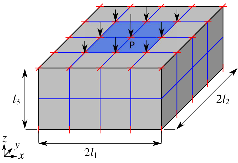
The model problem investigated here is a cube made of Neo-Hookean material undergoing large deformation. Geometry and boundary conditions are shown in Fig. 1 (c.f. [40]). Using the symmetry of the problem only a quarter of the cube is considered. In Tab. 1 the parameters of our main setup are found.

Figure 1: Cube under compression

Young’s module	$E$	$=90$	$\left[$\text{\,}\mathrm{N}\mathrm{/}\mathrm{m}\mathrm{m}\mathrm{{}^{2}}$\right]$
Poisson’s ratio	$\nu$	$=0.4999$
geometric dimensions	$l_{1},l_{2},l_{3}$	$=1$	$\left[$\text{\,}\mathrm{mm}$\right]$
Pressure	$F$	$=-320$	$\left[$\text{\,}\mathrm{N}\mathrm{/}\mathrm{m}\mathrm{m}\mathrm{{}^{2}}$\right]$

Table 1: Parameter configuration for the main precalculation.

To ensure a stable computation, the pressure is applied incrementally in time. 100 time steps are used until full loading is achieved For the computations itself the finite element analyse program FEAP[43] is used.

2.1 UQ for the Cube

Since the paper focuses on surrogate models for uncertainty quantification, cf. [42], as main application, our problem is extended, so that the parameters of our model problem lie in a range instead of having an assigned fixed value. Additionally, the units are omitted and the parameter ranges are set to

$$E\in\left[150,2000\right]\mbox{ and }l_{k}\in\left[0.95,1.05\right],\,k\in\left\{1,2,3\right\}.$$ (1)

For the remainder of the paper we will keep the boundaries for the geometric parameters constant, the Young’s modulus and the loading will change to save some computation time. To ease up notation in the following chapters, we also introduce the parameter space

$$\mathcal{S}=\left[0.95,1.05\right]^{3}\times\left[150,1000\right]$$ (2)

and take the liberty to enumerate our parameters

$$p_{k}=l_{k},\mbox{ for }k\in\left\{1,2,3\right\}\mbox{ and }p_{4}=E.$$ (3)

The problem of uncertainty quantification eases up, when only one scalar value is of interest. For our model problem the maximal deformation is chosen, which is measured in percentage of the initial height of the cube. This quantity of interest is denoted as $\varphi$. This leads us to the main task of this paper, which is to provide a mapping

$$\varphi:\mathcal{S}\to\mathbb{R},p\mapsto\varphi(p).$$ (4)

Once a mapping is found, it becomes feasible to estimate the first statistical moments of the quantity of interest, namely the mean and the variance, by means of a Monte Carlo method. Each parameter has a probability distribution, e.g. a uniform distribution over the range or a truncated normal distribution. We generate a finite discrete set $\mathcal{X}$ of random parameter configurations according to the respective distributions. Then, the sums

$$\mu=\frac{1}{|\mathcal{X}|}\sum_{p\in\mathcal{X}}\varphi(p)\mbox{ and }\sigma^{2}=\frac{1}{|\mathcal{X}|-1}\sum_{p\in\mathcal{X}}\left(\varphi(p)-\mu\right)^{2}$$ (5)

estimate the mean and the variance. Non-intrusive methods like multilevel Monte Carlo [16] or stochastic collocation [1] methods are superior to this method regarding the number of samples needed for an accurate estimation. But since the focus of this paper lies on the construction and investigation of reduction methods for the mapping (4) the standard Monte Carlo method is used throughout this paper. In the following chapters, the reduced models which provide this mapping are studied in detail. Then, then the resulting methods are employed for uncertainty quantification in Section 7.

3 Model reduction for the Neo Hooke equation

Model order reduction (MOR) in the context of FE means that the order of the model is reduced in order to save CPU time and memory [38]. For many applications this paves the way for indepth investigations of the problem at hand, because irrelevant parts of the model can be significantly reduced.

3.1 The problem

The discrete nonlinear equation system is obtained from a displacement-based finite element formulation

$$\mbox{\boldmath{$M$}}\ddot{\mbox{\boldmath{$U$}}}(t)+\mbox{\boldmath{$R$}}(\mbox{\boldmath{$U$}}(t))=\mbox{\boldmath{$P$}}(t),$$ (6)

where for static examples the $n\times 1$ nodal acceleration vector $\ddot{\mbox{\boldmath{$U$}}}(t)$ can be neglected. The $n\times n$ matrix $M$ represents the mass matrix and the $n\times 1$ vector $\mbox{\boldmath{$U$}}(t)$ the vector of nodal displacements. The external load is represented by the time-dependent $n\times 1$ vector $\mbox{\boldmath{$P$}}(t)$. With this assumption and Eq. (6) the residual vector $\mbox{\boldmath{$G$}}(\mbox{\boldmath{$U$}}(t))$ is defined as

$$\mbox{\boldmath{$G$}}(\mbox{\boldmath{$U$}}(t))\coloneqq\mbox{\boldmath{$R$}}(\mbox{\boldmath{$U$}}(t))-\mbox{\boldmath{$P$}}(t)=\mbox{$\bf 0$}.$$ (7)

The dependence on the time $t$ is from now on omitted in the notation. Commonly, the Newton-Raphson method is used to solve the nonlinear Equation (7).

3.2 Projection based MOR

One special kind of MOR is the projection based MOR, where the high dimensional equation system is projected to an equation system of smaller dimension $m$ [29]. This smaller equation system is solved and the solution is then projected back to the high dimensional space. Especially suitable is this procedure for problems, where the difference in displacement between time steps is well approximated by a linear combination of the basis $\mbox{\boldmath{$W$}}_{1},\ldots,\mbox{\boldmath{$W$}}_{m}$.

The dimension $m$ determines the accuracy and computational effort of the POD. With smaller $m$ the computational effort is reduced in exchange for accuracy. Usually, $m$ can be chosen to be much smaller than $n$, without substantial loss of accuracy.

Let $\Phi$ be the $n\times m$ projection matrix which serves for the projection from the $n$ dimensional space onto the $m$ dimensional space. Furthermore, let $\mbox{\boldmath{$U$}}_{\mathrm{red}}^{j}$ be the reduced $m\times 1$ displacement vector and

$$\mbox{\boldmath{$U$}}^{j}\approx\bar{\mbox{\boldmath{$U$}}}^{j}=\mbox{\boldmath{$\Phi$}}^{j}\;\mbox{\boldmath{$U$}}_{red}^{j}$$ (8)

be the unreduced $n\times 1$ displacement vector of the $j$th time step. Additionally, the tangential stiffness matrix $K$ can be projected as

$$\mbox{\boldmath{$K$}}_{T}(\mbox{\boldmath{$U$}}^{j})=\mbox{\boldmath{$\Phi$}}^{j}\mbox{\boldmath{$K$}}_{T}(\mbox{\boldmath{$U$}}_{red}^{j})\mbox{\boldmath{$\Phi$}}^{j~{}T}$$ (9)

where $\mbox{\boldmath{$K$}}_{T}(\mbox{\boldmath{$U$}}_{red}^{j})$ is the reduced tangential stiffness matrix. Applying Eq. (8) and Eq. (9) to the Taylor-Expansion Eq. (LABEL:eq:iterative_solution_alg) the dimension is reduced from $n$ to $m$:

$$\underbrace{\mbox{\boldmath{$\Phi$}}^{j~{}T}\mbox{\boldmath{$G$}}(\mbox{\boldmath{$\Phi$}}^{j}\mbox{\boldmath{$U$}}_{red,i}^{j})}_{\displaystyle{\mbox{\boldmath{$G$}}_{red}}}+\underbrace{\mbox{\boldmath{$\Phi$}}^{j~{}T}\mbox{\boldmath{$K$}}_{T}(\mbox{\boldmath{$\Phi$}}^{j}\mbox{\boldmath{$U$}}_{red,i}^{j})\mbox{\boldmath{$\Phi$}}^{j}}_{\displaystyle{\mbox{\boldmath{$K$}}_{t,red}}}\Delta\mbox{\boldmath{$U$}}_{red,i+1}^{j}=\mbox{$\bf 0$}.$$ (10)

The success of this procedure relies on the right choice of the $m$ dimensional space and thus respectively on the proper construction of the projection matrix $\Phi$. Alternative methods to construct the projection matrix are the modal basis reduction method [35] and the load-dependent Rith method [34, 29]. For the type of problems which are her of interest, the POD has been shown to be the most efficient [37].

3.3 Proper orthogonal decomposition (POD)

The proper orthogonal decomposition method (POD) is based on the singular value decomposition (SVD). It is mainly used in fields like turbulent flow, stochastics, image or signal analysis [9, 24]. In the field of mechanics [7, 26, 31] different approaches to employ POD were presented.

The POD is built upon “snapshots” which are the result of unreduced calculations. Thus, it is important to perform the unreduced calculations with parameter configurations which in the end represent the full behaviour of the system. Each time step of our precalculation results into a displacement vector $\mbox{\boldmath{$U$}}^{j}$ with the dimension $n\times 1$. These displacement vectors are gathered in the $n\times l$ snapshot matrix $\mbox{\boldmath{$D$}}=\left[\mbox{\boldmath{$U$}}^{1}~{}\mbox{\boldmath{$U$}}^{2}~{}...~{}\mbox{\boldmath{$U$}}^{l}\right]~{}\in\mathbb{R}^{n\times l}.$ The SVD $\mbox{\boldmath{$D$}}=\mbox{\boldmath{$W$}}\mbox{\boldmath{$\Sigma$}}\mbox{\boldmath{$V$}}^{T}=\sum_{k=1}^{l}\sigma^{k}\mbox{\boldmath{$W$}}^{k}\mbox{\boldmath{$V$}}^{k^{T}}$ is used to generate a suitable orthonormal basis where $\mbox{\boldmath{$W$}}=(\mbox{\boldmath{$W$}}^{1}~{}\mbox{\boldmath{$W$}}^{2}~{}...~{}\mbox{\boldmath{$W$}}^{l})~{}\in\mathbb{R}^{n\times l}$ and $\mbox{\boldmath{$V$}}=(\mbox{\boldmath{$V$}}^{1}~{}\mbox{\boldmath{$V$}}^{2}~{}...~{}\mbox{\boldmath{$V$}}^{n})~{}\in\mathbb{R}^{l\times n}$ are orthonormal matrices. $\Sigma$ is a diagonal matrix which contains the singular values ($\sigma^{k}$) which are always positive, ordered decreasingly. The projection matrix $\Phi$ can be obtained as

$$\mbox{\boldmath{$\Phi$}}=\left(\mbox{\boldmath{$W$}}^{1}~{}\mbox{\boldmath{$W$}}^{2}~{}...~{}\mbox{\boldmath{$W$}}^{m}\right)~{}~{}\in\mathbb{R}^{n\times m}.$$ (11)

The projection matrix $\Phi$ is used to solve the nonlinear Eq. (7) on a lower dimensional space.

4 Adaptive proper orthogonal decomposition (APOD)

When using POD, it is assumed that the solution lies in a linear space, spanned by the basis functions $\mbox{\boldmath{$W$}}^{1}\ldots\mbox{\boldmath{$W$}}^{m}$. Therefore, each linear combination of these basis functions is a possible solution. In general, all snapshots are used to construct the projection matrix $\Phi$. However, in particular in the context of non-linear behaviour, not all snapshots might be representative of the current deformation behaviour. This makes the POD inefficient, since more basis vectors than necessary are used [20].

It is imaginable that in each time step the respective solution would be matched better by a different but smaller basis. Thus, a simple principle to choose a proper subset of snapshots is introduced which are then employed in the construction of such a matched basis. We call this method adaptive proper orthogonal decomposition.

4.1 Principle

For geometrically nonlinear problems we suggest to introduce a projection matrix $\bar{\mbox{\boldmath{$\Phi$}}}$ which depends on the maximal current displacement $\bar{u}_{max}$. Investigating geometric nonlinear problems we propose to introduce a projection matrix $\bar{\mbox{\boldmath{$\Phi$}}}$ depending on the maximal current deformation $\bar{u}_{max}$, the bar represents the current time step and the maximum displacement is defined as

$$\bar{u}_{max}=\|\bar{\mbox{\boldmath{$U$}}}\|_{\infty}.$$ (12)

The snapshot vectors are sorted with respect to the maximum displacement

$$||\mbox{\boldmath{$U$}}^{1}||_{\infty}\leq||\mbox{\boldmath{$U$}}^{2}||_{\infty}\leq...\leq||\mbox{\boldmath{$U$}}^{l}||_{\infty}.$$ (13)

The current maximal displacement $u_{max}$ is compared with the maximal displacement of each of the snapshots $||\mbox{\boldmath{$U$}}^{1}||_{\infty}~{}...~{}||\mbox{\boldmath{$U$}}^{l}||_{\infty}$. The index of the snapshot, which fits the maximum displacement best is denoted as

$$b(\bar{u}_{max})=\underset{i\epsilon\{1,...,l\}}{\operatornamewithlimits{argmin}}~{}\left(|(||\mbox{\boldmath{$U$}}||_{\infty}-\bar{u}_{max})|\right).$$ (14)

The snapshots close to the current maximal displacement are chosen and it is expected that these snapshots represent the behaviour of the current state well. To ensure that the snapshots around the index $b$ are still in the range of available snapshots the index of the first taken snapshot is defined as

$$a=\max{\left[0;\min\left(l-o;b-\left\lfloor\frac{o}{2}\right\rfloor\right)\right]}$$ (15)

which ensures that the snapshots exist. The number of considered snapshots is called $o$. In [25] it is shown that

$$o=ms$$ (16)

is a good choice for $o$, where $s$ is the number of precalculations and $m$ the number of modes. In the case that

$$l-o<b-\left\lfloor\frac{o}{2}\right\rfloor$$

available snapshots do not lead to good results, we recommend to generate snapshots with larger deformations. After determining $a$ one can construct a suitable snapshot matrix

$$\bar{\mbox{\boldmath{$D$}}}=\left(\mbox{\boldmath{$U$}}^{a+1}~{}\mbox{\boldmath{$U$}}^{a+2}~{}...~{}\mbox{\boldmath{$U$}}^{a+o}\right)\in\mathbb{R}^{n\times m}$$ (17)

for the current timestep. With a singular value decomposition of the current snapshot matrix

$$\bar{\mbox{\boldmath{$D$}}}=\bar{\mbox{\boldmath{$\lambda$}}}\bar{\mbox{\boldmath{$\Sigma$}}}\bar{\mbox{\boldmath{$V$}}}^{T}=\sum_{k=1}^{l}\bar{\sigma}^{k}\bar{\mbox{\boldmath{$\lambda$}}}^{k}\bar{\mbox{\boldmath{$V$}}}^{k^{T}}$$ (18)

the projection matrix $\bar{\mbox{\boldmath{$\Phi$}}}$ for the current timestep is created as

$$\bar{\mbox{\boldmath{$\Phi$}}}=\left(\bar{\mbox{\boldmath{$\lambda$}}}^{1}~{}\bar{\mbox{\boldmath{$\lambda$}}}^{2}~{}...~{}\bar{\mbox{\boldmath{$\lambda$}}}^{m}\right),$$ (19)

where $\bar{\mbox{\boldmath{$\Sigma$}}}$ contains the singular values in decreasing order.

4.2 Numerical results

The parameters for the precalculation can be found in Tab. 1. In a first step a change of the Young’s modulus is considered for different number of modes. Therefore, all other parameters are the same as the precalculation found in Tab. 1. In the following different models will be compared. To do so a relative error between two models X and Y is introduced as

$$\epsilon_{\mathrm{X,Y}}=\frac{\varphi_{\mathrm{X}}-\varphi_{\mathrm{Y}}}{\varphi_{\mathrm{X}}}.$$ (20)

The result of the FEAP simulation is denoted as $\varphi_{\mathrm{full}}$ where phi is defined in Section 2 and serves here as a placeholder for our quantities of interest. The results of APOD and POD are denoted as $\varphi_{\mathrm{POD}}$ and $\varphi_{\mathrm{APOD}}$, respectively. The abbreviation (A)POD is used, if both APOD and POD are referred to. The error $\epsilon_{\mathrm{full,(A)POD}}$ is used to assess the accuracy of APOD and POD.

Figure 2: Comparison of the accuracy of POD and APOD for a variation of the Young’s modulus $E$. The number appending “POD” or “APOD” represents the number of used modes.

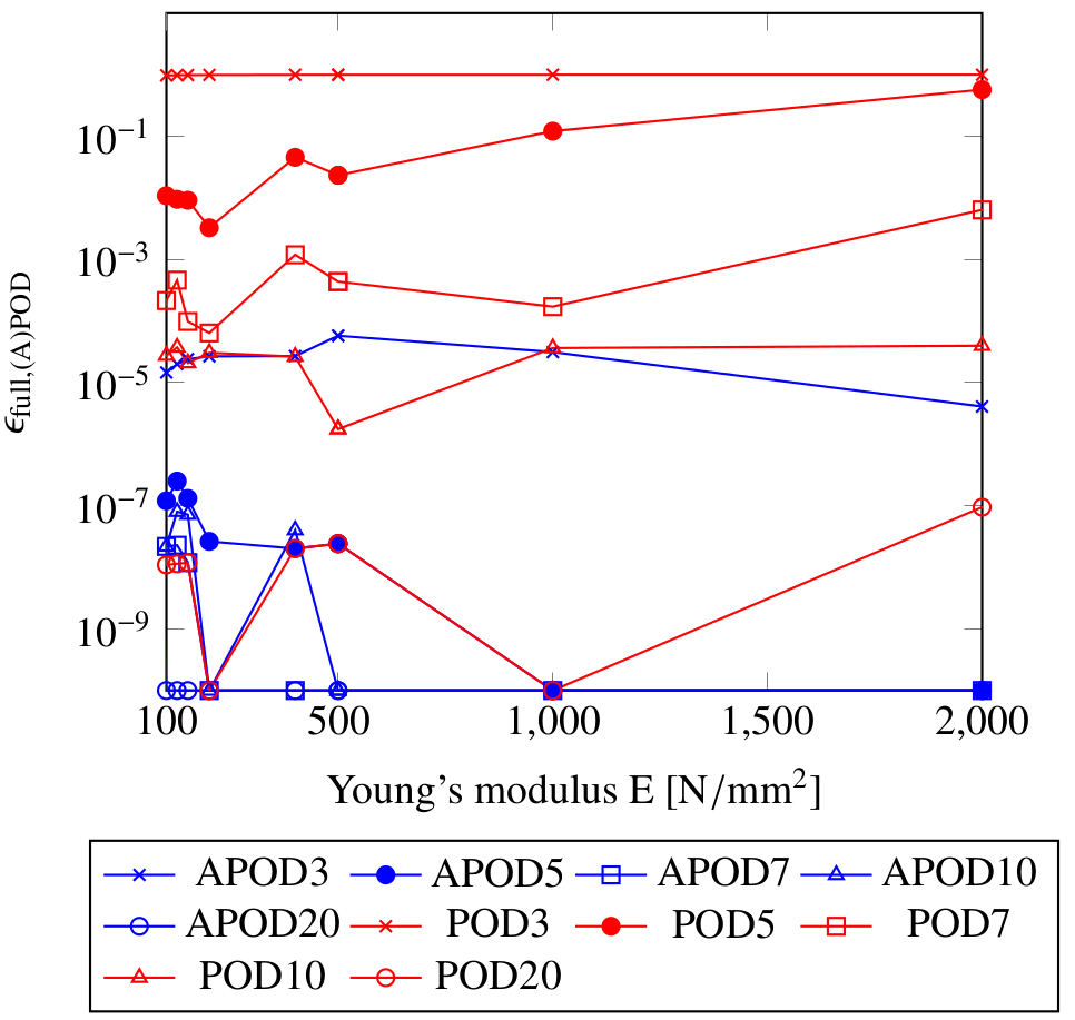
In Fig. 2 POD and APOD are compared. APOD with $m=3$ modes is denoted by “APOD3”, POD with $m=5$ modes is denoted by “POD5”. The other configurations are denoted accordingly. In this example it can be seen that the new APOD method with the same number of modes is for all cases significantly more accurate than the POD method, since the snapshots are carefully selected to fit the current situation in every time step. Figure 2 also shows that the APOD method with $m=3$ modes yields approximately the same accuracy as POD with $m=10$ modes. APOD is more expensive due to the fact that for each time step a singular value decomposition is computed. On the other hand, each singular value decomposition is much cheaper since $\dim{(\bar{\mbox{\boldmath{$D$}}})}\leq\dim{(\mbox{\boldmath{$D$}})}$. The comparison of the computational time $t_{\mathrm{POD}}$ for POD and the computational time $t_{\mathrm{APOD}}$ for APOD shows that the cost are almost equal for the same number of modes, with $t_{APOD}/t_{POD}\in\left[1.03,1.05\right]$. Comparing the computation times which yield approximately the same accuracy shows that with $t_{POD10}/t_{APOD3}\approx 1.63$ the POD requires 63% more computation time.

Figure 3: Comparison of the absolute $L2$ error

Figure 4: Comparison of the absolute QoI error

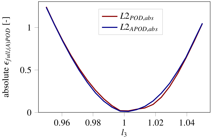
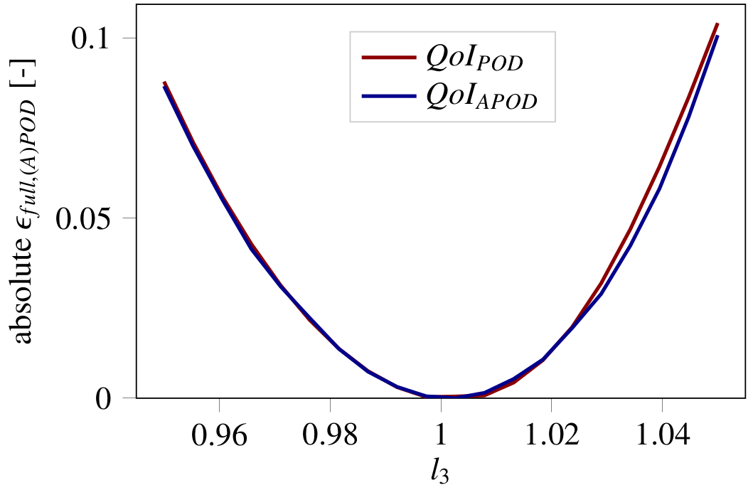
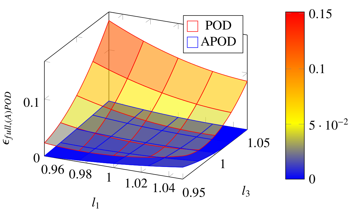
POD and APOD yields accurate results if the Young’s modulus is stiffer than the Young’s modulus of the precalculation. For our problem the dimensions of the cube are added as parameters. Each dimension varies between $l_{1},l_{2},l_{3}\in[0.95,1.05]$. In Fig. 3 and 4 two points are observed. First, both POD and APOD are not able to capture the influence of change in the dimensions with the precomputation at hand. Second, both measures reflect this. Whereas, the measure via the QoI is easier to compute. Thus, in the following we will focus on the error measurement using the QoI. To improve POD and APOD sensibly chosen precomputations are needed. Stiffer Young’s moduli do not provide additional information, since these are equivalent to the effect of weaker loading and softer material, which are already captured in the first time steps. For the dimensions the strongest effect on the quantity of interest is expected for the extremal values. Thus, the parameter configurations from Tab. 2 are taken for the precalculations.

Table 2: Material parameters and different sets of the precalculations

Material	Parameters	Pressure
Neo-Hookean	$E=200$\text{\,}\mathrm{N}\mathrm{/}\mathrm{m}\mathrm{m}\mathrm{{}^{2}}$$	$-0,320$\text{\,}\mathrm{N}\mathrm{/}\mathrm{m}\mathrm{m}\mathrm{{}^{2}}$$
	$\nu=0.4999$
Sets:
1.    $l_{1}=0.95,~{}l_{2}=0.95,~{}l_{3}=0.95$
2.    $l_{1}=1.05,~{}l_{2}=0.95,~{}l_{3}=0.95$
3.    $l_{1}=0.95,~{}l_{2}=1.05,~{}l_{3}=0.95$
4.    $l_{1}=0.95,~{}l_{2}=0.95,~{}l_{3}=1.05$

In Fig. 5 the results for the new precalculations are shown. The error $\epsilon_{\mathrm{full,(A)POD}}$ is plotted over the width $l_{1}$ and the height $l_{3}$ for $l_{2}=1.00$ and $E=200$. For all tested parameter configuration APOD has a higher accuracy.

$l_{2}=1$ is selected, since this choice is not covered by the precalculations directly. A variation of $l_{2}$ leads to similar results with the same set of snapshots.

Figure 5: Comparison of the accuracy of POD and APOD for uncertain parameters: $l_{2}=1.00$, $E=200$ and $10$ modes

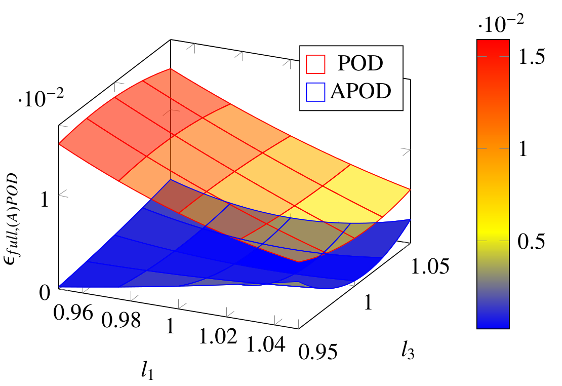
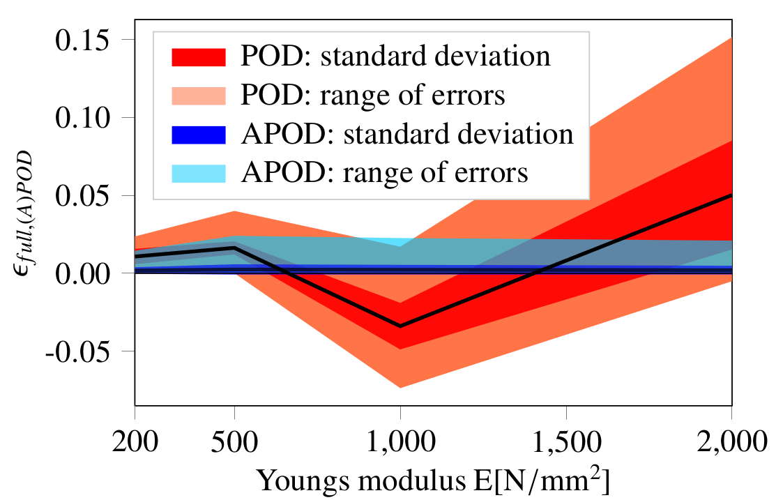
Raising Young’s modulus to a value of $E=2000\left[\frac{N}{mm^{2}}\right]$ leads to worse accuracy of POD. This is observed in Fig. 6. The error $\epsilon_{\mathrm{full,POD}}$ rises up to $15\%$, while the maximal error $\epsilon_{\mathrm{full,APOD}}$ stagnates at $2\%$. It is therefore interesting to investigate the accuracy of POD and APOD for a variation of Young’s modulus. In Fig. 8 this relation is presented. The modulus is fixed and the dimensions are covered by $1000$ samples. The ranges and the standard deviation of the errors $\epsilon_{\mathrm{full,POD}}$ and $\epsilon_{\mathrm{full,APOD}}$ are plotted. Both, range and standard deviation of $\epsilon_{\mathrm{full,APOD}}$ remain constantly smaller than the respective range and standard deviation of $\epsilon_{\mathrm{full,POD}}$.

Figure 6: Comparison of the accuracy of POD and APOD for uncertain parameters: $l_{2}=1.05$, $E=2000$ and 10 modes

Figure 7: Comparison of $\epsilon_{\mathrm{full,(A)POD}}$ for 1000 random samples.

Figure 8: Comparison of mean, deviation and range of errors for the range of uncertain parameters between POD and APOD

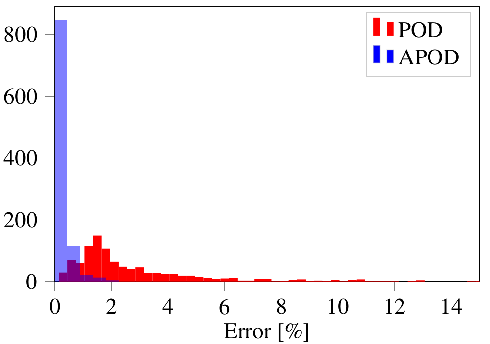
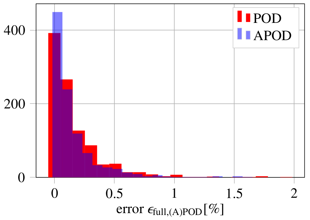
Comparing the classic POD with APOD shows that the APOD increases the accuracy of the calculation significantly with the same or a smaller number of modes. This becomes particularly clear in Fig. 7, where the error is measured for $1000$ random parameter configurations. It requires a singular value decomposition for each time step. However, each SVD is cheaper than the SVD for all snapshots at once. By using APOD the computation cost of $\varphi$ is reduced drastically.

Nonetheless, for accurate Monte Carlo simulations usually millions of samples are required, thus the reduction of computational cost is not sufficient. In the next chapters a more specialized method and the synergies with (A)POD are investigated.

5 Hierarchical tensor approximation (HTA)

One way to further reduce the complexity of the mapping from the high-dimensional parameter space to a manageable number of quantities of interest is the hierarchical Tucker decomposition [18, 22]. To introduce this decomposition in a simple way, we discretise the parameter space $\mathcal{S}$ on a tensorized grid, meaning that a finite number of points are taken for each parameter and every combination of these points are taken. For our purposes $N$ equidistant points in each parameter direction are sufficient. Therefore, we denote for the parameters $l_{i}$ and $E$ the variations

$$l_{i,k}=0.95+k\cdot\frac{0.1}{N-1}\;\text{and}\;E_{k}=100+k\cdot\frac{100}{N-1},$$

with $k\in\left\{0,\ldots,N-1\right\}$, and the resulting grid as $\mathcal{D}$. We describe the corresponding indice set $\mathcal{I}$ by

$$(i_{1},i_{2},i_{3},i_{4})\in\mathcal{I}=\mathcal{I}_{\left\{1\right\}}\times\mathcal{I}_{\left\{2\right\}}\times\mathcal{I}_{\left\{3\right\}}\times\mathcal{I}_{\left\{4\right\}}=\left\{0,1,\ldots,N-1\right\}^{4}.$$

Evaluating the mapping on this grid $\mathcal{D}$ yields a $4$-th order tensor array, where each entry $\Phi\left(i,j,k,l\right)$ is the maximal displacement for the parameter combination $(l_{1,i},l_{2,j},l_{3,k},E_{l})$. Analogously, we denote the tensor arrays $\Phi_{\mathrm{POD}}$ and $\Phi_{\mathrm{APOD}}$ which stem from the prediction given by POD and APOD, respectively.

For the HT decomposition of these tensor arrays each parameter is associated with a mode. For example the parameter $E$ is associated with the mode $\left\{4\right\}$ and the parameters $l_{1},l_{2}$ and $l_{3}$ with the modes $\left\{1\right\},\left\{2\right\}$ and $\left\{3\right\}$. We start with a set of modes $\left\{1,\ldots,d\right\}$. Then, this set of modes is split into $2$ subsets. The resulting subsets are recursively split until each subset only contains one mode. Thus, the resulting structure is a binary tree with sets of modes in every vertex. This structure is denoted as dimension tree $\mathcal{T}_{D}$, the root of this tree as $D=\left\{1,2,3,4\right\}$ and the set of leaves as $\mathcal{L}=\left\{\left\{1\right\},\left\{2\right\},\left\{3\right\},\left\{4\right\}\right\}$. In Figure 9 we find the dimension tree which is used throughout this paper. A dimension tree is a concept to describe the structure of a HT tensor. When describing an algorithm for the HT format, the dimension tree is used to navigate us through the different parts of the HT tensor.

The second concept needed is the matricisation of a tensor, which is just a reordering of the tensor entries into a matrix. The first two indices $(i_{1},i_{2})$ and the remaining two indices $(i_{3},i_{4})$ are renumbered lexicographically with a single index $i$ and a single index $j$, the matricisation of the tensor $A$ is denoted as

$$\mathcal{M}^{\left\{1,2\right\}}\left(A\right)_{i,j}\coloneqq A\left(i_{1},i_{2},i_{3},i_{4}\right).$$

For an accessible introduction to matricisations, see [19]. In the same way, by assigning one single index $i$ to a set of indices corresoponding to the respective modes in the dimension tree and another indice $j$ to the remaining indices of the tensor, the matricisations is constructed for each node in the dimension tree. Therefore, the matricisation $\mathcal{M}^{\left\{1,2,3,4\right\}}(A)$ is assigned to the root. This matrix consists of a single column, which contains all tensor entries. For the first leaf, the indice $i$ is associated with $(i_{1})$ and the indice $j$ with $(i_{2},i_{3},i_{4})$. This yields the matricisation $\mathcal{M}^{\left\{1\right\}}(A)$. In a way, this sets the first parameter in proportion to all remaining parameters. For example, if it holds

$$A(i_{1},i_{2},i_{3},i_{4})=c_{i_{1}},\quad\forall(i_{2},i_{3},i_{4})\in\mathcal{I},$$

the first parameter is unrelated to the rest. This leads to a rank $1$ matrix for the matricisation associated with this leaf. The rank is an indication on how strongly one parameter relates to the remaining parameter. With the association of the rank of a matricisation to the respective mode set $t\in\mathcal{T}_{D}$, it yields the definition of the hierarchical rank

$$\mathbf{k}=\left(k^{t}\right)_{t\in\mathcal{T}_{D}},\quad k^{t}\coloneqq\mathrm{rank}\left(\mathcal{M}^{t}\left(A\right)\right),\quad t\in\mathcal{T}_{D}.$$

The set of tensors with a certain hierarchical rank $\mathbf{k}$ is denoted as

$$\mathcal{H}_{\mathbf{k}}\coloneqq\left\{A\in\mathbb{R}^{\mathcal{I}}:\mathrm{rank}\left(\mathcal{M}_{t}\left(A\right)\right)\leq k_{t},t\in\mathcal{T}_{D}\right\}.$$

It is not to be expected that a tensor is included in $\mathcal{H}_{\mathbf{k}}$. Therefore, the goal is rather, to find an approximation $\tilde{A}\in\mathcal{H}_{\mathbf{k}}$ for a tensor $A$. In [18] an quasi-optimal algorithm was developed based on singular value decomposition (SVD). For the resulting tensor $A_{\mathcal{H}-\mathrm{SVD}}\in\mathcal{H}_{\mathbf{k}}$ applies

$$\|A-A_{\mathcal{H}-\mathrm{SVD}}\|_{2}\leq\sqrt{2d-3}\min_{A_{\mathrm{best}}\in\mathcal{H}_{\mathbf{k}}}\|A-A_{\mathrm{best}}\|_{2}.$$

The use of a SVD is expensive, in the sense that all entries of a matricisation are used. A data sparse method to find a low rank approximation of a matrix is the skeleton or cross approximation [17]. The basic idea is to only use a subset of rows and columns of the matrix. Let $M\in\mathbb{R}^{\mathcal{I}_{1}\times\mathcal{I}_{2}}$, $\mathcal{P}\subset\mathcal{I}_{1}$ and $\mathcal{Q}\subset\mathcal{I}_{2}$, then the cross approximation reads

$$\tilde{M}\coloneqq M|_{\mathcal{I}_{1}\times\mathcal{Q}}~{}S^{-1}~{}M|_{\mathcal{P}\times\mathcal{I}_{2}},$$

where $S$ is the submatrix that arises at the intersections of the chosen rows and columns. This method only employs the entries of the rows and columns, thus the computation of most of the entries in the matrix are spared. Finding those pivot sets $\mathcal{P}$ and $\mathcal{Q}$ is possible in an adaptive fashion, cf. [5], meaning that the algorithm proceeds until a cross approximation with a certain accuracy is found or until a certain rank is reached.

Figure 9: The arrangement of the stored data in a hierarchical tucker format.

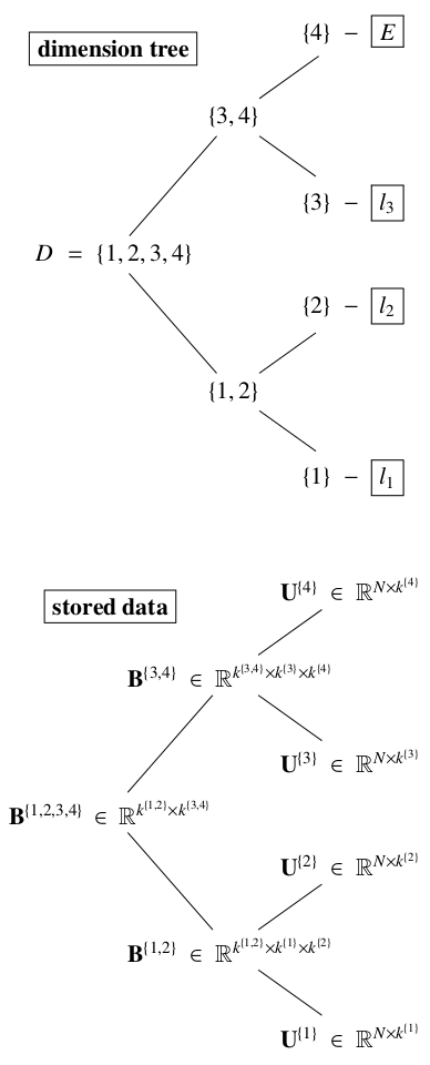
With help of this algorithm, a low rank approximation is found for each matricisation in the dimension tree. This yields column spaces for each node in $T_{D}$. The important columns $\left(U^{\left\{\mu\right\}}_{j}\right)_{j\in\left\{1,\ldots,k^{\mu}\right\}}$ found for the matricisations on the leafes are simply stored colum-wise in a matrix $\mathbf{U}^{\left\{\mu\right\}}$, with $\mu\in\left\{1,2,3,4\right\}$. We denote these as frames. One level higher, the important columns are found by the cross approximation method for a submatrix of $\mathcal{M}^{t}(A)$. But instead of storing these columns, we compute and store the coefficients $\left(\mathbf{B}^{t}\right)_{i,j,k}$, which approximate $U^{t}_{j}$ with linear combinations of kronecker products of the columns $U^{s_{1}}_{k}\otimes U^{s_{2}}_{l}$, with $\mathrm{sons}\left(t\right)=\left\{s_{1},s_{2}\right\}$. More precisely, these linear combinations read

$$\left(U^{t}\right)_{\cdot,j}=\sum_{j_{1}=1}^{k_{s_{1}}}\sum_{j_{2}=1}^{k_{s_{2}}}\left(\mathbf{B}^{t}\right)_{j,j_{1},j_{2}}\left(U^{s_{1}}\right)_{\cdot,j_{1}}\otimes\left(U^{s_{2}}\right)_{\cdot,j_{2}},\quad j\in\mathcal{I}^{t},$$ (21)

for all $t\in\mathcal{T}_{D}\setminus\mathcal{L}$. Each transfer tensor $\mathbf{B}$ is computed by a series of projections between linear spaces. In condensed form it reads

$$\left(\mathbf{B}^{t}\right)_{j,\cdot,\cdot}=S^{-1}_{s_{1}}\left(\mathcal{M}^{t}(A)\right)_{(\cdot,\cdot),j}S^{-1}_{s_{1}}.$$

With these transfer tensors $\mathbf{B}^{t}$, the frames and Eq. (21), it yields a low rank approximation for a tensor array, given that the ranks in each node are small. We denote this approximation in the following as hierarchical Tucker approximation (HTA) and the algorithm for finding the HTA as generalized cross approximation. We have some control over the construction by setting the size of the submatrices and by setting the accuracy or the maximal rank for each cross approximation. This method of constructing a HT tensor is elaborated in [3].

The transfer tensors and frames are the only data that is needed to be stored for an hierarchical tucker approximation. Let

$$k=\max_{t\in\mathcal{T}_{D}}k^{t},$$

then the upper bound reads $4\cdot N\cdot k+2k^{3}+k^{2}$ for the number of stored elements from Figure 9. For $N=100$ and $k=5$, it yields $2275$ elements compared to $10^{8}$ elements in a full tensor.

With Eq. (21) we have access to each entry of $U^{D}$ and therefore to each entry of the $\mathcal{H}$ tensor. For $(i_{1},i_{2},i_{3},i_{4})\in\mathcal{I}$ we pick the respective row $v^{\left\{k\right\}}\coloneqq\mathbf{U}_{i_{k},\cdot}$ and compute

$$\left(w^{\left\{1,2\right\}}\right)_{j}=\sum_{j_{1}=1}^{k^{\left\{1\right\}}}\sum_{j_{2}=1}^{k^{\left\{2\right\}}}\left(\mathbf{B}^{\left\{1,2\right\}}\right)_{j,j_{1},j_{2}}v^{\left\{1\right\}}_{j_{1}}v^{\left\{2\right\}}_{j_{2}}.$$

In the same fashion, we compute $w^{\left\{3,4\right\}}$. Finally, the entry is computed by

$$\mathcal{H}(i_{1},i_{2},i_{3},i_{4})=\sum_{j_{1}=1}^{k^{\left\{1,2\right\}}}\sum_{j_{2}=1}^{k^{\left\{3,4\right\}}}\left(\mathbf{B}^{\left\{1,2,3,4\right\}}\right)_{j_{1},j_{2}}w^{\left\{1,2\right\}}_{j_{1}}w^{\left\{3,4\right\}}_{j_{2}}.$$

Thus, this evaluation needs $2k+4$ matrix vector multiplications.

6 HTA for the cube under compression

Next, the mapping (4) is approximated by the means of HTA. For HTA an already available mapping is needed, e.g. $\varphi_{\mathrm{full}}$, which is deduced from a full FEAP simulation. Other choices are the reduced (A)POD models. The reduced mappings are denoted as $\varphi_{\mathrm{POD}}$ and $\varphi_{\mathrm{APOD}}$ and the respective approximating mappings in hierarchical Tucker format are denoted as $\varphi_{\mathcal{H}_{\mathrm{full}}},\varphi_{\mathcal{H}_{\mathrm{POD}}}$ and $\varphi_{\mathcal{H}_{\mathrm{APOD}}}$.

We employ the generalized cross approximation as briefly described in Chapter 5 with random matrices of size $8$ for all tensor arrays, as long as the matricisation allows it. If the number of rows or columns of the matricisation is smaller, the smaller number is used for the size of the respective random sub matrix. The cross approximation for each matricisation is then executed in an adaptive manner with a tolerance of $10^{-6}$ which means that the distance between the cross approximation and the actual matrix is less than $10^{-6}$ in each entry of the selected rows and columns. This is not a guarantee for accuracy but at least a well established heuristic.

For each tensor array $\Phi$ which is deduced from the mapping $\varphi$, we examine different resolutions of the parameter space and a different number of finite elements, namely $N\in\left\{4,8,16,32,64\right\}$ and $N_{\mathrm{FEM}}\in\left\{2^{3},4^{3},8^{3}\right\}$. To reduce computation time and to ensure the stability of the input for the HTA the loading is reduced by $80\%$. The range of the Young’s modulus is chosen to be in the range $\left[100,200\right]$.

	Construction time [s]			Used entries
sampling	mesh			mesh
rate	$2^{3}$	$4^{3}$	$8^{3}$	$2^{3}$	$4^{3}$	$8^{3}$
4	44	272	5866	167	161	169
8	84	552	11135	338	341	335
16	123	798	16266	496	488	496
32	186	1230	24673	750	752	752
64	313	2066	41549	1264	1264	1264

Table 3: Construction times of a HTA and the respective number of used entries.

The construction times are found for different numbers of samplings $N$ and $3$ different resolutions of the mesh are listed in Tab. 3. All computations were performed on a cluster with 2x Intel Xeon X5690 processors with 2x6 CPU cores with 3.47 GHz and 48GB RAM. Each column shows the same trend. The number of finite elements determines the magnitude of the computational time needed, where the sampling rate only changes the computational time in a sub-linear fashion. This is not a high price to pay, especially when compared to the number of used entries. Obviously, independently of the number of finite elements, the percentage of used entries of the tensor array drops rapidly with increasing sampling rate. This means that a higher resolution in the parameter space leads to a higher compression of the encapsulated information by the HTA. Around $10^{3}$ evaluations are needed for $N=64$, independently of the number of finite elements used. This indicates that the structure of the mapping $\phi$ is suitable for an approximation in a hierarchical Tucker format, stemming from simulations with different accuracies.

Figure 10: Estimated absolute HTA error $\delta_{\mathrm{full},\mathcal{H}_{\mathrm{full}}}$ from $100$ random parameters and $N_{\mathrm{FEM}}=8^{3}$.

6.1 Approximation quality

Figure 11: Distribution of all relative errors $\epsilon_{\mathrm{full},\mathcal{H}_{\mathrm{full}}}$. Estimated from $1000$ random parameters on the tensorized grid.

Figure 12: Distribution of all relative errors $\epsilon_{\mathrm{full},\mathrm{(A)POD}}$. Estimated from $1000$ random parameters on the tensorized grid.

Figure 13: Distribution of all relative errors $\epsilon_{\mathrm{APOD},\mathcal{H}_{\mathrm{(A)POD}}}$. Estimated from $1000$ random parameters on the tensorized grid.

Figure 14: Distribution of all relative errors $\epsilon_{\mathrm{full},\mathcal{H}_{\mathrm{APOD}}}$ . Estimated from $1000$ random parameters on the tensorized grid.

		std
	mean	deviation	max	min
	[%]	[%]	[%]	[%]
$\epsilon_{\mathrm{full,POD}}$	0.1641	0.2372	1.9854	-0.0519
$\epsilon_{\mathrm{full,APOD}}$	0.1543	0.2047	1.6533	-0.0173
$\epsilon_{\mathrm{POD},\mathcal{H}_{\mathrm{POD}}}$	0.0030	0.0189	0.1586	-0.0712
$\epsilon_{\mathrm{APOD},\mathcal{H}_{\mathrm{APOD}}}$	0.0012	0.1618	2.4481	-0.8481
$\epsilon_{\mathrm{full},\mathcal{H}_{\mathrm{full}}}$	0.0000	0.0002	0.0011	-0.0014
$\epsilon_{\mathrm{full},\mathcal{H}_{\mathrm{POD}}}$	0.1611	0.2316	2.0459	-0.0573
$\epsilon_{\mathrm{full},\mathcal{H}_{\mathrm{APOD}}}$	0.1555	0.2506	2.4506	-0.766

Table 4: Errors for different methods from $1000$ random parameters on the tensorized grid.

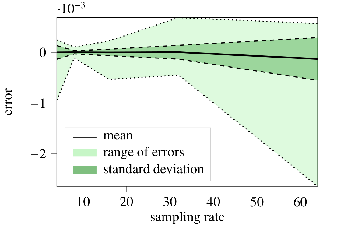
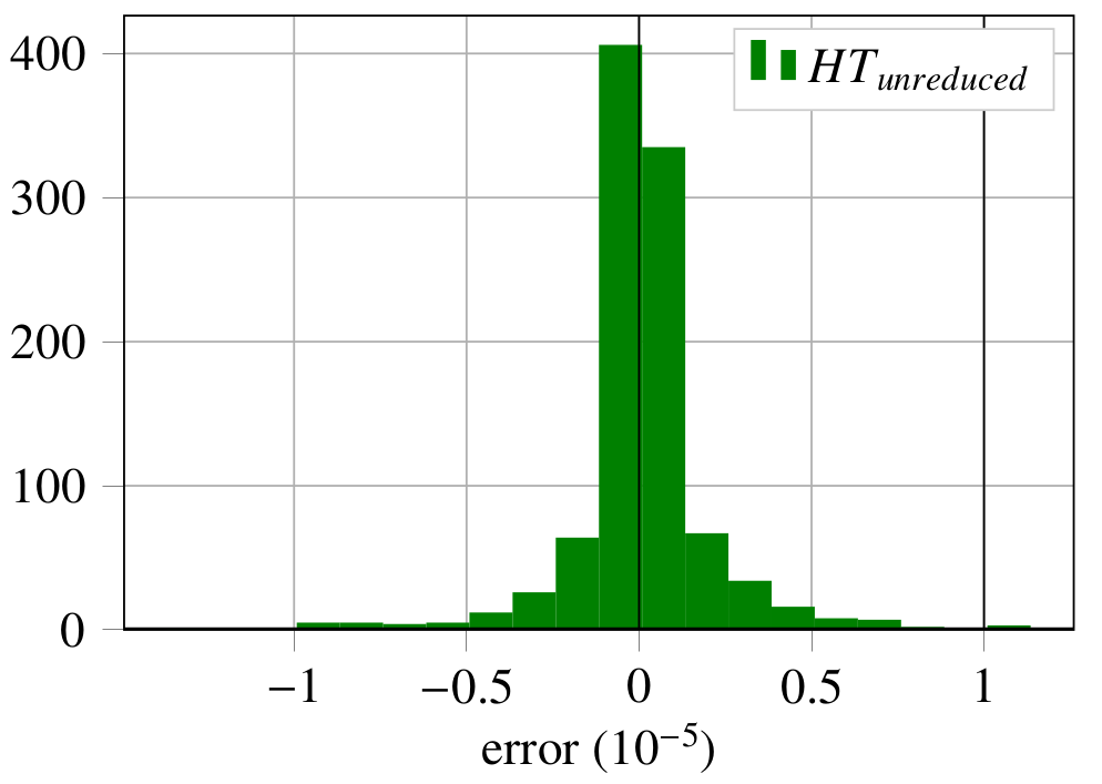
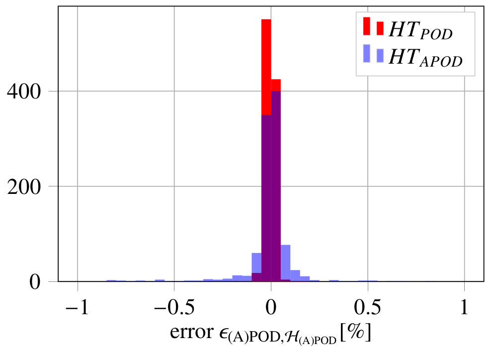
More interesting is the approximation quality of the HTA. To estimate the quality we examine the distributions of various errors. For each distribution $1000$ random parameter combinations $(l_{1},l_{2},l_{3},E)\in\mathcal{D}$ are used. In Fig. 10 the range of errors is plotted including the mean over the different sampling rates and $N_{\mathrm{FEM}}=8^{3}$. It is observed that the maximal error lies around the magnitude $10^{-4}$. In relation to the displacement, which lies between $20\%$ and $30\%$, the maximal error is six magnitudes smaller. Accordingly, it is observed in Fig. 11 that the maximal relative error

$$\epsilon_{\mathrm{full},\mathcal{H}_{\mathrm{full}}}(p)=\frac{\varphi_{\mathrm{full}}(p)-\varphi_{\mathcal{H}_{\mathrm{full}}}(p)}{\varphi_{\mathrm{full}}(p)}$$

is of magnitude $10^{-6}$ in most cases.

The next error observed is the relative error

$$\epsilon_{\mathrm{(A)POD}}(p)=\frac{\varphi_{\mathrm{(A)POD}}(p)-\mathcal{H}_{\mathrm{F}}(p)}{\varphi_{\mathrm{(A)POD}}(p)}.$$

Here, Fig. 13 shows that the maximal relative error is smaller than $0.15\%$, which is a satisfactory result for certain applications. It suggests that the reduced model produces a mapping, which is less suitable for this kind of low rank approximation. In comparison to the HTA of the unreduced model the error is $3$ orders of magnitude worse.

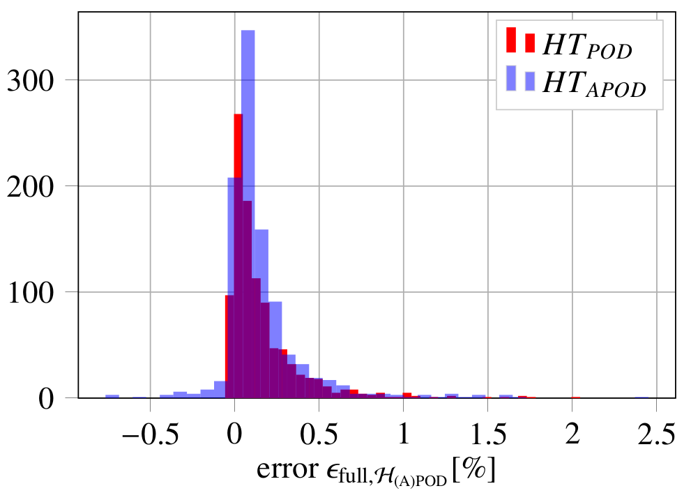
Whenthe HTA of a reduced model to approximate the mapping $\varphi_{\mathrm{F}}$ is used, the approximation errors of the reduced model and of the HTA are added. Empirically, this is observed with the relative error $\epsilon_{\mathrm{full},\mathcal{H}_{\mathrm{(A)POD}}}(p)$,which is found in Fig. 14. A majority of relative errors are smaller than $1\%$, which is still a sufficient approximation quality for some applications.

An overview of all relative errors is found in Table 4. APOD yields the better results, although it scatters more. Note that these errors were measured for a fifth of the loading. Therefore, the errors $\epsilon_{\mathrm{full,POD}}$ and $\epsilon_{\mathrm{full,APOD}}$ do not comply with the errors found in Sec. 4. With a fifth of the original loading the cube shows less pronounced non-linear behaviour. Therefore, to obtain the same error level, about the same number of modes are used for POD and APOD.

The HTA is seemingly better suited for POD than for APOD. If the HTA is constructed from (A)POD, the mean relative error to the unreduced model is just the sum of the means of $\epsilon_{\mathrm{POD},\mathcal{H}_{\mathrm{(A)POD}}}$ and $\epsilon_{\mathrm{full},\mathcal{H}_{\mathrm{(A)POD}}}$. The relative errors of HTA and the (A)POD approximation are two magnitudes apart from each other. Overall, it is feasible to surrogate $\varphi_{\mathrm{(A)POD}}$ with $\varphi_{\mathcal{H}_{\mathrm{(A)POD}}}$.

Of course, there is plenty of room for improvement and many angles to approach this insufficiency. It would be easily possible to increase the ranks of the HTA or the number of modes and snapshots of the POD. Both ideas would lead to an increase of computational cost, but the balance between these cost and the approximation quality is its own task for every application, where HTA and POD methods are used in combination.

Instead of constructing the approximation $\mathcal{H}_{\mathrm{(A)POD}}$ of the (A)POD model we will employ the HTA to improve the used snapshots and therefore the (A)POD model itself in the next chapter. This is to our knowledge the first attempt in literature.

6.2 Finding snapshots with HTA

In the previous chapters, the POD and APOD model was built upon snapshots, which were carefully chosen from an understanding of the model problem. Therefore, one question at hand is, if it is possible to improve the POD or APOD method, by finding better snapshots with the help of the HTA of the unreduced method. Since the approximation quality of HTA for the unreduced model has a high accuracy, the CPU time effort can be significantly reduced by using HTA instead of the full FE model.

One way to assess the approximation quality of the (A)POD model is the comparison to the unreduced FE model. With this measure at hand it is possible to find parameter configurations where the discrepancy between FE model and (A)POD model is especially large. New snapshots are then generated for this particular parameter configurations, thus reducing the discrepancy between FE and (A)POD model. One iteration of this procedure may be be written down as

• Build a (A)POD model $\varphi_{\mathrm{(A)POD},k}(p)$ from an initial set of snapshots $\mathcal{S}_{k}$

• Provide a measure $r:\mathcal{D}\to\mathbb{R}$ for the discrepancy between reduced and unreduced model

• Find $p^{*}=\underset{p\in\mathcal{D}}{\operatorname{argmax~{}}}|r(p)|$

• Generate the snapshots $\mathcal{S}(p^{*})$ and enrich the used set of snapshot $\mathcal{S}_{k+1}=\mathcal{S}_{k}\cup\mathcal{S}(p^{*})$

This step may be repeated until a fixed number of snapshots is found or a certain tolerance is reached. Step $3$ is especially expensive, since the parameter space may be high dimensional. Additionally, for an accurate measure of the discrepancy evaluations of the full model are needed. To mitigate these costs, we propose to use HTA as a surrogate model of the residual $r$ in each step. Therefore, let the residual be denoted as

$$r_{k}:\mathcal{D}\to\mathbb{R}:p\mapsto\varphi_{\mathcal{H}_{\mathrm{full}}}(p)-\varphi_{\mathrm{(A)POD},k}(p),$$ (22)

where $\varphi_{\mathrm{(A)POD},k}(p)$ denotes the $k$-th reduced model from a successively constructed set of models. Naturally, we start this series with $\varphi_{\mathrm{(A)POD},0}(p)\equiv 0$ which is equivalent to an empty set of snapshots $\mathcal{S}_{0}=\emptyset$ and implies $r_{0}(p)=\varphi_{\mathcal{H}_{\mathrm{full}}}(p)$. The main step is the third step which consists of the computation of $\max_{p\in\mathcal{D}}\left|r_{k}(p)\right|$.

The maximum is estimated by finding the maxima in alternating directions iteratively. Heuristically, in our case this gives a good estimation for the maximum. To improve the snapshot set it is not necessary to find the global maximum.

Once a maximum (global or local) is determined, this leads to a parameter configuration where the discrepancy between reduced and unreduced model is high. Exactly this parameter configuration is then used to generate a new set of snapshots $\mathcal{S}_{k+1}$, leading to $\varphi_{\mathrm{(A)POD},k+1}$. These steps are repeated iteratively until a certain tolerance is fulfilled or a maximum number of iterations is reached.

We perform this procedure for POD and APOD, with underlying a FE model with $4^{3}$ elements and use a HTA with a sampling rate of $64$ points per parameter. In our experiments this coarse FE model lead to very similar parameter configurations as a finer model. This strategy makes the procedure of this section feasible in practise to provide a sensible selection of snapshots for more accurate models.

In Tab. 5, the devolopment of the absolute maximum with each iteration is found. The decline of the residual is significant until it stagnates after the fifth iteration. This, most probably, leads back to the approximation error of the HTA for the residual $r_{k}$.

k	POD	APOD
0	34.628	34.6262
1	11.8444	1.52712e+08
2	0.145506	0.0933674
3	0.206719	0.178969
4	0.0496022	0.0337002
5	0.0352917	0.0618711

Table 5: The development of $\max_{p\in\mathcal{D}}\left|r_{k}(p)\right|$.

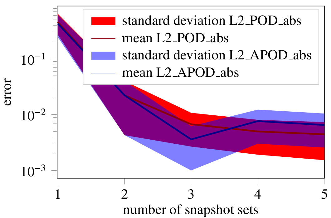
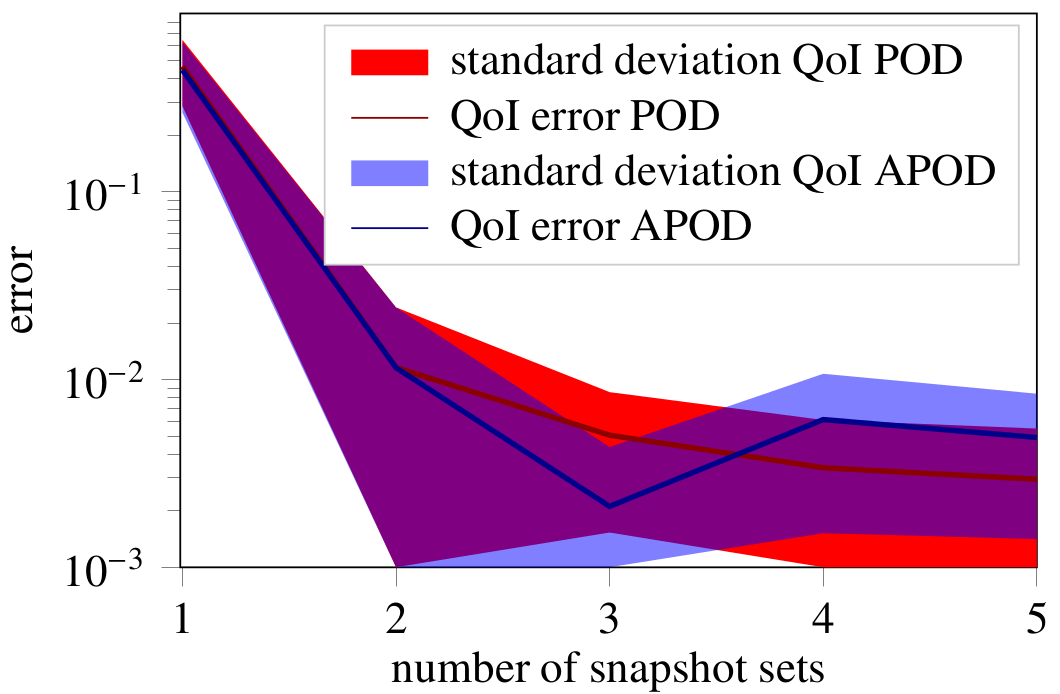
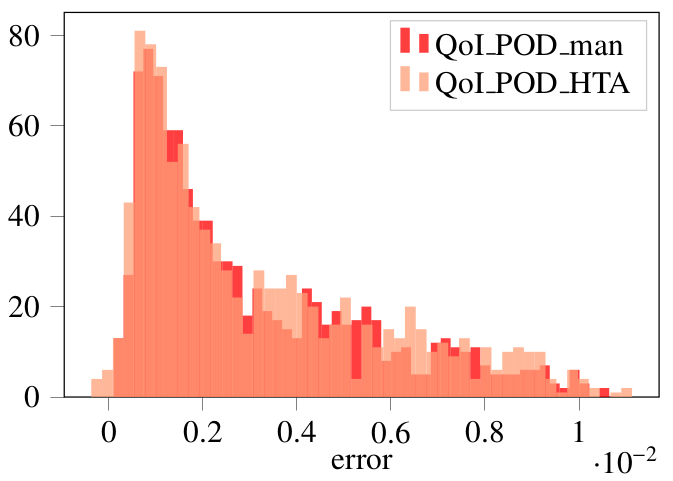
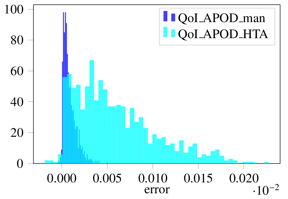
To compare these new models with the models in Sec. 4, we generate random parameters and compute the difference in the quantity of interest as one measurement for the quality of the reduced model, as well as the $L^{2}$ error as a second measurement. We observe in Fig. 15 and Fig. 16, that the whole procedure is working for both measurements. For APOD we find that there is a kink for both measurements. On the other hand, a comparison with the manually chosen snapshots in Fig. 18 shows, that the HTA chosen snapshots are significantly worse for APOD. One reason could be, that the interesting parameter configurations are found at the boundary of the parameter space, but the HTA lacks accuracy at the boundaries. The reason for this is the manner in which the HTA is constructed. Since the generalized cross approximation takes submatrices of the respective matricizations, the parameters on the boundary space are usually not hit upon. For this simple problem it is practicable to choose suitable snapshots. In more challenging situations this task becomes more difficult. In those cases, the procedure above could suggest parameter configurations for a set of quantities of interest, so that the choice of snapshots becomes feasible.

Figure 15: Development of the $L_{2}$-error between the full model and the (A)POD model with a successively enriched snapshot set.

Figure 16: Development of the QoI-error between the full model and the (A)POD model with a successively enriched snapshot set.

Figure 17: Distribution of the errors for two different POD models from $1000$ samples. With manually chosen snapshots and with systematically found snapshots using HTA.

Figure 18: Distribution of the errors for two different APOD models from $1000$ samples. With manually chosen snapshots and with systematically found snapshots using HTA.

Once a suitable reduced model is found, it may be used for a variety of application. Since the main application in this paper is uncertainty quantification in form of a Monte Carlo estimation of the mean and variance, we will discover in the following chapter how to perform this with the HTA.

7 Comparison - HTA and APOD

In this paper, three levels of modeling are considered. The first level is the FEM model, the second level is the POD model deduced from the FEM model and the third level is the low rank approximation in the hierarchical tensor format. Each level is in some sense more specialized and carries less information. E.g., the FEM model is able to deal with changes in the geometry, whereas POD is only able to deal with the changes covered by the snapshots. This effect is shown in Section 4, more precisely, in Fig. 3. The POD model provides the displacement in every node of the cube, thus most quantities of interest which depend on the displacement are easily computed. In contrast, the HTA is only suitable to approximate a single quantity of interest. Consequently, another HTA has to be established, if another quantity of interest has to be investigated. The advantage of this highly specialized approximation is the low cost of computation later on. Construction times, the time needed to evaluate $100$ random parameters as well as the convergence behaviour for the estimation of the mean and variance are analyzed and compared in the following (see Tab. 6).

	constr. time [$\text{\,}\mathrm{s}$]	$1000$ eval. [$\text{\,}\mathrm{s}$]
FEM	-	32722.4
POD	130.89	19869.7
APOD	130.89	22320.8
HTA of FEM	41497.5	0.245135
HTA of POD	25260.6	0.241672
HTA of APOD	28343.8	0.238908

Table 6: An overview of the computation times for construction and evaluation of (A)POD and HTA. With $8^{3}$ finite elements.

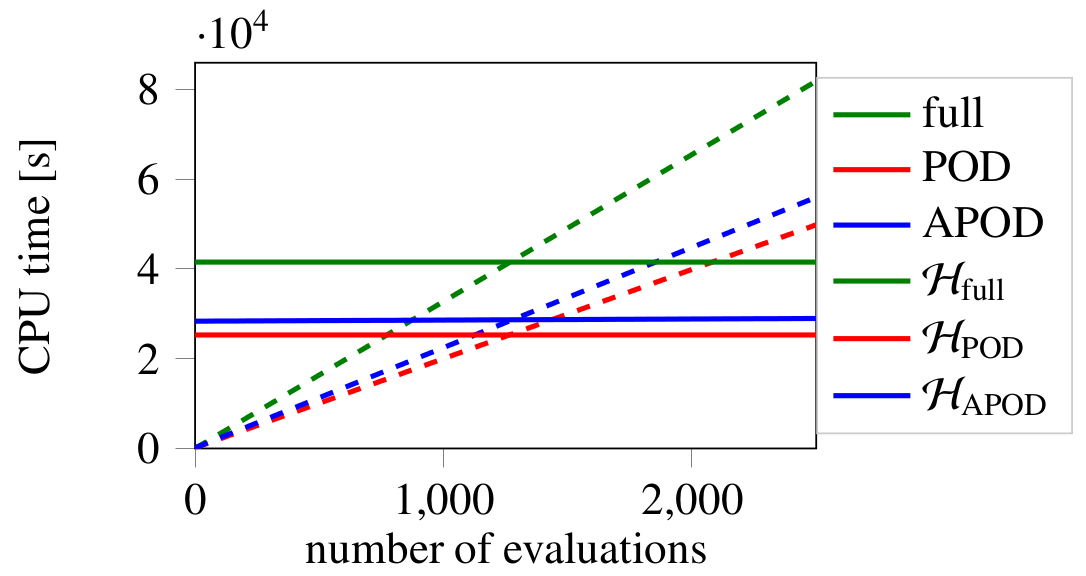
Naturally, the construction time of the unreduced FEM model is zero. The construction time of APOD and POD is relatively low, since only a handful of FE simulations are needed to generate the snapshots. For the construction of the HTA, around $10^{3}$ evaluations have to be carried out, therefore the construction time is very high in comparison, even if POD is used as basis. Note, that the times given in Tab. 6 are subject to fluctation, since the number of entries needed to construct a HTA depends on the random submatrices in the computation of the generalized cross approximation. Further, it has to be taken into account that for theevaluation of a POD or APOD model an iterative solver with an adaptive number of iteration steps is used. Yet, the orders of magnitude are consistent for all performed experiments.

The high construction times of HTA pay off, as it is seen for the cost of $100$ evaluations. In Fig. 19 the total CPU time is plotted over the number of evaluations. For instance for 1000 evaluations, the use of HTA does not really pay off, because the construction time for establishing the $\mathcal{H}-$Tensor is very high in comparison to the CPU time needed to comput the results of 500 evaluations. Already for 2500 evaluations, the picture has changed to the opposite. Please note that a number of 2500 evaluations is easily reached and in the context of uncertainty quantification a very small number of evaluations.

Figure 19: Comparison of the computational time over the number of evaluations

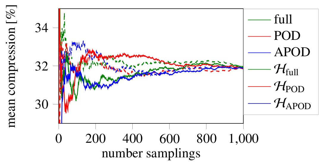
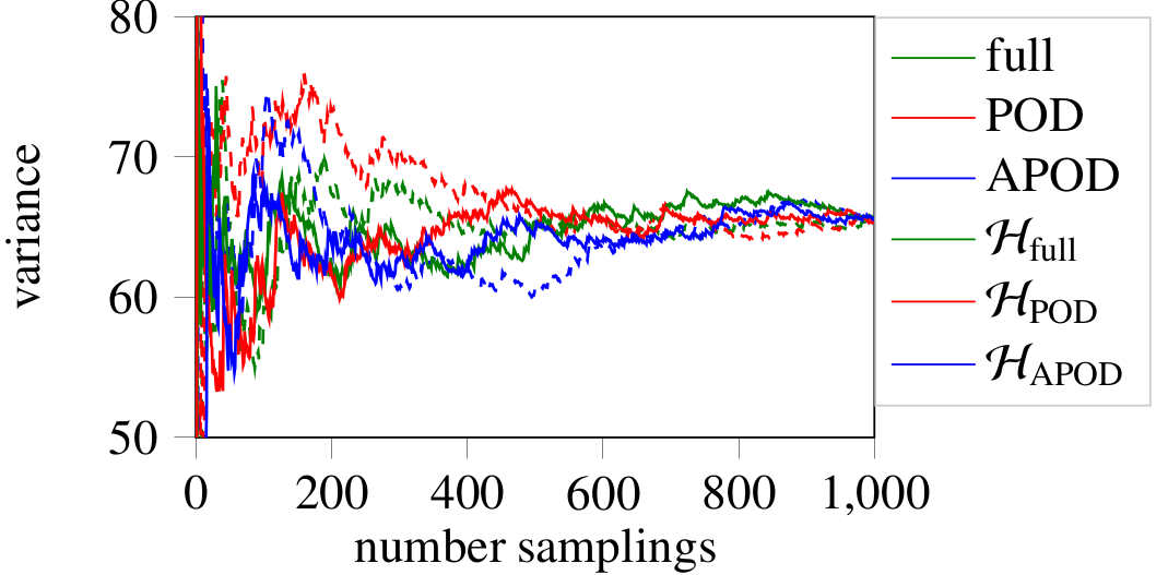
The mean and the variance of the maximal displacement are shown in Fig. 20 and Fig. 21, respectively For both, the mean and the variance, it can be observed that all models converge rapidly to a similar value. The differences of the mean values in Tab. 7 are in the same magnitude as the errors found in Tab. 4.

Figure 20: Convergence to the mean for all models up to $1000$ samplings.

Figure 21: Convergence to the variance for all models up to $1000$ samplings.

		std
	mean	deviation	max	min
	[%]	[%]	[%]	[%]
$\varphi_{\mathrm{full}}$	31.936	8.1107	50.6728	20.6467
$\varphi_{\mathrm{POD}}$	31.8818	8.0875	50.0193	20.6248
$\varphi_{\mathrm{APOD}}$	31.8853	8.0926	50.1861	20.6199
$\varphi_{\mathcal{H}_{\mathrm{full}}}$	31.936	8.1107	50.6727	20.6467
$\varphi_{\mathcal{H}_{\mathrm{POD}}}$	31.8828	8.088	50.0455	20.6186
$\varphi_{\mathcal{H}_{\mathrm{APOD}}}$	31.886	8.0967	50.1872	20.6196

Table 7: QoI for different methods from $1000$ random parameters on the tensorized grid.

8 Conclusion and Outlook

In this work three levels of modeling were presented. The original FE model which is here considered as full model was first reduced by (adaptive) proper orthogonal decomposition and then by low rank approximation in hierarchical tucker format. It should be emphasized that the procedure is applicable to arbitrarily geometrically and materially non-linear problems. The present paper is, however, restricted to Neo Hookean behaviour, where uncertainties in geometric and material parameters were investigated.

First of all, both model reduction methods were assessed with respect to their approximation quality. It was discovered that the accuracy of the A(POD) has to be improved by additional snapshots. An efficient procedure to find these additional snapshots by means of a novel combination of a greedy algorithm with HTA was developed. The accuracy obtained from the automatically chosen snapshots was compared with the result of the manually chosen snapshots. Obviously, the method is promising, in particular for complex examples where the manual choice of the snapshots is very difficult.

Beside the approximation quality, the construction and evaluation times of (A)POD and HTA were compared. The results indicate that using a low rank approximation of a (A)POD model is a viable combination of methods. Since the error $\epsilon_{\mathrm{(A)POD},\mathcal{H}_{\mathrm{(A)POD}}}$ is several magnitudes smaller than the error $\epsilon_{\mathrm{full},\mathrm{(A)POD}}$, the approximation $\varphi_{\mathcal{H}_{\mathrm{(A)POD}}}$ becomes a useful surrogate for $\varphi_{\mathrm{(A)POD}}$ which in turn is a surrogate for the full model. The relation between construction times of $\mathcal{H}_{\mathrm{(A)POD}}$ and $\mathcal{H}_{\mathrm{full}}$ is proportional to the relation of evaluation times of an (A)POD and a full simulation. Whereas the evaluation time of a low rank tensor is negligible in relation to one evaluation of the (A)POD model. For large scale problems both the relation of construction and evaluation times will improve significantly in favour of this strategy.

In the development of this work, many ideas for future work emerged. These ideas were excluded here, in order to focus on the relation between POD and HTA. With regard to modern methods in uncertainty quantification, like multi-level and quasi Monte Carlo methods, stochastic collocation and stochastic Galerkin methods, one idea would be to incorporate our reduced models. In terms of polymorphic uncertainty quantification, an attempt to incorporate fuzzy-stochastic numbers or other non-probabilistic methods could improve the representation of epistemic uncertainties.

9 References

References

- Babuška et al. [2007] Babuška, I., Nobile, F., Tempone, R., 2007. A stochastic collocation method for elliptic partial differential equations with random input data. SIAM Journal on Numerical Analysis 45 (3), 1005–1034.
- Ballani and Grasedyck [2015] Ballani, J., Grasedyck, L., 2015. Hierarchical tensor approximation of output quantities of parameter-dependent pdes. SIAM/ASA Journal on Uncertainty Quantification 3 (1), 852–872.
- Ballani et al. [2013] Ballani, J., Grasedyck, L., Kluge, M., 2013. Black box approximation of tensors in hierarchical tucker format. Linear algebra and its applications 438 (2), 639–657.
- Barrault et al. [2004] Barrault, M., Maday, Y., Nguyen, N. C., Patera, A. T., 2004. An ‘empirical interpolation’method: application to efficient reduced-basis discretization of partial differential equations. Comptes Rendus Mathematique 339 (9), 667–672.
- Bebendorf [2000] Bebendorf, M., 2000. Approximation of boundary element matrices. Numerische Mathematik 86 (4), 565–589.
- Bellman [2013] Bellman, R., 2013. Dynamic programming. Courier Corporation.
- Berkley et al. [2004] Berkley, J., Turkiyyah, G., Berg, D., Ganter, M., Weghorst, S., 2004. Real-time finite element modeling for surgery simulation: An application to virtual suturing. IEEE Transactions on visualization and computer graphics 10 (3), 314–325.
- Berkooz et al. [1993] Berkooz, G., Holmes, P., Lumley, J. L., 1993. The proper orthogonal decomposition in the analysis of turbulent flows. Annual review of fluid mechanics 25 (1), 539–575.
- Chatterjee [2000] Chatterjee, A., 2000. An introduction to the proper orthogonal decomposition. Current science, 808–817.
- Chinesta et al. [2011] Chinesta, F., Ladeveze, P., Cueto, E., 2011. A short review on model order reduction based on proper generalized decomposition. Archives of Computational Methods in Engineering 18 (4), 395.
- Corveleyn and Vandewalle [2017] Corveleyn, S., Vandewalle, S., 2017. Computation of the output of a function with fuzzy inputs based on a low-rank tensor approximation. Fuzzy Sets and Systems 310, 74–89.
- De Lathauwer et al. [2000] De Lathauwer, L., De Moor, B., Vandewalle, J., 2000. A multilinear singular value decomposition. SIAM journal on Matrix Analysis and Applications 21 (4), 1253–1278.
- Dolgov and Scheichl [2017] Dolgov, S., Scheichl, R., 2017. A hybrid alternating least squares–tt cross algorithm for parametric pdes. arXiv preprint arXiv:1707.04562.
- Eftang et al. [2011] Eftang, J. L., Knezevic, D. J., Patera, A. T., 2011. An hp certified reduced basis method for parametrized parabolic partial differential equations. Mathematical and Computer Modelling of Dynamical Systems 17 (4), 395–422.
- Espig et al. [2014] Espig, M., Hackbusch, W., Litvinenko, A., Matthies, H. G., Wähnert, P., 2014. Efficient low-rank approximation of the stochastic galerkin matrix in tensor formats. Computers & Mathematics with Applications 67 (4), 818–829.
- Giles [2013] Giles, M. B., 2013. Multilevel monte carlo methods. In: Monte Carlo and Quasi-Monte Carlo Methods 2012. Springer, pp. 83–103.
- Goreinov et al. [1997] Goreinov, S. A., Tyrtyshnikov, E. E., Zamarashkin, N. L., 1997. A theory of pseudoskeleton approximations. Linear algebra and its applications 261 (1-3), 1–21.
- Grasedyck [2010] Grasedyck, L., 2010. Hierarchical singular value decomposition of tensors. SIAM Journal on Matrix Analysis and Applications 31 (4), 2029–2054.
- Grasedyck and Hackbusch [2011] Grasedyck, L., Hackbusch, W., 2011. An introduction to hierarchical (h-) rank and tt-rank of tensors with examples. Computational Methods in Applied Mathematics Comput. Methods Appl. Math. 11 (3), 291–304.
- Haasdonk et al. [2011] Haasdonk, B., Dihlmann, M., Ohlberger, M., 2011. A training set and multiple bases generation approach for parameterized model reduction based on adaptive grids in parameter space. Mathematical and Computer Modelling of Dynamical Systems 17 (4), 423–442.
- Hackbusch [2012] Hackbusch, W., 2012. Tensor spaces and numerical tensor calculus. Vol. 42. Springer Science & Business Media.
- Hackbusch and Kühn [2009] Hackbusch, W., Kühn, S., 2009. A new scheme for the tensor representation. Journal of Fourier analysis and applications 15 (5), 706–722.
- Hitchcock [1927] Hitchcock, F. L., 1927. The expression of a tensor or a polyadic as a sum of products. Journal of Mathematics and Physics 6 (1-4), 164–189.
- Holmes [2012] Holmes, P., 2012. Turbulence, coherent structures, dynamical systems and symmetry. Cambridge university press.
- Kastian and Reese [2018] Kastian, S., Reese, S., 2018. An adaptive way of choosing significant snapshots for the proper orthogonal decomposition. submitted to IUTAM bookseries.
- Kerschen et al. [2005] Kerschen, G., Golinval, J.-c., Vakakis, A. F., Bergman, L. A., 2005. The method of proper orthogonal decomposition for dynamical characterization and order reduction of mechanical systems: an overview. Nonlinear dynamics 41 (1), 147–169.
- Kolda and Bader [2009] Kolda, T. G., Bader, B. W., 2009. Tensor decompositions and applications. SIAM review 51 (3), 455–500.
- Krysl et al. [2001a] Krysl, P., Lall, S., Marsden, J. E., 2001a. Dimensional model reduction in non-linear finite element dynamics of solids and structures. International Journal for numerical methods in engineering 51 (4), 479–504.
- Krysl et al. [2001b] Krysl, P., Lall, S., Marsden, J. E., 2001b. Dimensional model reduction in non-linear finite element dynamics of solids and structures. International Journal for numerical methods in engineering 51 (4), 479–504.
- Kunisch and Volkwein [2008] Kunisch, K., Volkwein, S., 2008. Proper orthogonal decomposition for optimality systems. ESAIM: Mathematical Modelling and Numerical Analysis 42 (1), 1–23.
- Lenaerts et al. [2001] Lenaerts, V., Kerschen, G., Golinval, J.-C., 2001. Proper orthogonal decomposition for model updating of non-linear mechanical systems. Mechanical Systems and Signal Processing 15 (1), 31–43.
- Litvinenko and Matthies [2012] Litvinenko, A., Matthies, H. G., 2012. Uncertainty quantification in numerical aerodynamic via low-rank response surface. PAMM 12 (1), 781–784.
- Matthies et al. [2016] Matthies, H. G., Zander, E., Rosić, B. V., Litvinenko, A., 2016. Parameter estimation via conditional expectation: a bayesian inversion. Advanced modeling and simulation in engineering sciences 3 (1), 24.
- Mollemans et al. [2005] Mollemans, W., Schutyser, F., Nadjmi, N., Suetens, P., 2005. Very fast soft tissue predictions with mass tensor model for maxillofacial surgery planning systems. In: International Congress Series. Vol. 1281. Elsevier, pp. 491–496.
- Nickell [1976] Nickell, R. E., 1976. Nonlinear dynamics by mode superposition. Computer Methods in Applied Mechanics and Engineering 7 (1), 107–129.
- Oseledets [2011] Oseledets, I. V., 2011. Tensor-train decomposition. SIAM Journal on Scientific Computing 33 (5), 2295–2317.
- Radermacher and Reese [2013] Radermacher, A., Reese, S., 2013. A comparison of projection-based model reduction concepts in the context of nonlinear biomechanics. Archive of Applied Mechanics 83 (8).
- Radermacher and Reese [2014] Radermacher, A., Reese, S., 2014. Model reduction in elastoplasticity: proper orthogonal decomposition combined with adaptive sub-structuring. Computational Mechanics 54 (3), 677–687.
- Radermacher and Reese [2016] Radermacher, A., Reese, S., 2016. Pod-based model reduction with empirical interpolation applied to nonlinear elasticity. International Journal for Numerical Methods in Engineering 107 (6), 477–495.
- Reese et al. [2000] Reese, S., Wriggers, P., Reddy, B., 2000. A new locking-free brick element technique for large deformation problems in elasticity. Computers & Structures 75 (3), 291–304.
- Sachs and Volkwein [2010] Sachs, E. W., Volkwein, S., 2010. Pod-galerkin approximations in pde-constrained optimization. GAMM-Mitteilungen 33 (2), 194–208.
- Smith [2013] Smith, R. C., 2013. Uncertainty quantification: theory, implementation, and applications. Vol. 12. Siam.
- Taylor [2000] Taylor, R. L., 2000. Feap-a finite element analysis program.