Networks with point like nonlinearities

Abstract

We study static nonlinear waves in networks described by a nonlinear Schrödinger equation with point-like nonlinearities on metric graphs. Explicit solutions fulfilling vertex boundary conditions are obtained. Spontaneous symmetry breaking caused by bifurcations is found.

I Introduction

Modelling wave and particle transports in branched structures is an important problem with applications in many subjects of contemporary physics, such as optics, condensed matters, complex molecules, polymers and fluid dynamics. Mathematical treatment of such problems is reduced to solving different partial differential equations (PDEs) on so-called metric graphs. These are set of one-dimensional bonds, with assigned lengths. The connection rule of the bonds is called topology of the graph and is described in terms of the adjacency matrix Uzy1 ; Exner15 . Linear and nonlinear wave equations on metric graphs attracted much attention recently and they are becoming a hot topic Hadi1 -Noja19 .

Solving wave equations on metric graphs requires imposing boundary conditions at the branching points (graph vertices). In case of linear wave equations, e.g., for linear Schrödinger equation the main requirement for such boundary conditions is that they should keep self-adjointness of the problem Kost , while for nonlinear PDEs one needs to use other fundamental conservation laws (e.g., energy, norm, momentum, charge, etc) for obtaining vertex boundary conditions Zarif ; Our1 ; KarimNLDE . Energy and norm conservation was used to derive vertex boundary conditions for the nonlinear Schrödinger equation (NLSE) on metric graphs in Zarif , where exact solutions were obtained and integrability of the problem was shown under certain constraints. In Our1 a similar study was done for the sine-Gordon equation on metric graphs. Soliton solutions of a nonlinear Dirac equation on metric graphs have been obtained in KarimNLDE . Static solitons in networks were studied in the Refs. Adami2011 -Adami16 by solving stationary nonlinear Schrödinger equations on metric graphs. Other wave equations on metric graphs have been studied recently in Karim2018 . Modelling nonlinear waves and solitons in branched structures and networks provides powerful tool for tunable wave, particle, heat and energy transport in different practically important systems, such as branched optical fibres, carbon nanotube networks, branched polymers and low-dimensional functional materials.

Here we consider a Schrödinger equation with point-like nonlinearity on metric graphs. NLSE with pointlike nonlinearity can be implemented in dual-core fiber Bragg gratings as well as in the ordinary fibers Malomed3 and Bose-Einstein condensates confined in double-well traps Malomed4 ; Malomed5 . A similar problem on a line with double-delta type nonlinearity was considered earlier in Malomed1 ; Malomed2 , where explicit solutions were derived. On the basis of numerical analysis, it was shown that symmetric states are stable up to a spontaneous symmetry breaking bifurcation point. From a fundamental viewpoint it would be interesting to see the difference between solutions of the problem on the line and networks, as the topology of a network may cause additional effects. Here, we use the methods of Malomed1 to obtain explicit solutions of our problem. Degenerate spontaneous symmetry breaking bifurcations are also obtained.

The paper is organized as follows. In the next section formulation of the problem for metric star graph and the derivation of the vertex boundary conditions are presented. In Section III we obtain exact analytical solutions of the problem and formulate constraints for integrability. Numerical results and analysis of bifurcation is also presented in this section. Finally, Section IV presents some concluding remarks.

II Vertex boundary conditions

Consider a metric star graph consisting of three semi-infinite bonds, $b_{1}\sim(-\infty;0),\,b_{3}\sim(0;+\infty),\,b_{3}\sim(0;+\infty)$ (see, Fig. 1).

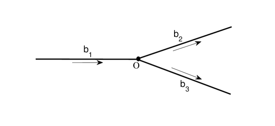
Figure 1: Metric star graph

On each bond of this graph the NLSE with variable nonlinearity coefficient, $g_{j}(x)$ can be written as

$$i\frac{\partial\psi_{j}}{\partial t}=-\frac{1}{2}\frac{\partial^{2}\psi_{j}}{\partial x^{2}}+g_{j}(x)|\psi_{j}|^{2}\psi_{j},$$ (1)

where $j=1,2,3$ denotes the bond number.

To solve Eq. (1), one needs to impose vertex boundary conditions (VBC), which can be derived, e.g., from norm and energy conservations laws. The norm and energy are given respectively by

$$N=\underset{j=1}{\overset{3}{\sum}}\underset{b_{j}}{\int}|\psi_{j}(x)|^{2}dx,$$ (2)

and

$$H=\frac{1}{2}\underset{j=1}{\overset{3}{\sum}}\underset{b_{j}}{\int}\left(\left|\frac{\partial\psi_{j}}{\partial x}\right|^{2}+g_{j}(x)|\psi_{j}|^{4}\right)dx.$$ (3)

From $\dot{N}=0$ and $\dot{H}=0$ and using $\psi_{1},\,\frac{\partial\psi_{1}}{\partial x}\to 0$ as $x\to-\infty$ and $\psi_{2,3},\,\frac{\partial\psi_{2,3}}{\partial x}\to 0$ as $x\to+\infty$, we obtain the following vertex boundary conditions (at $x=0$)

$${\bf Im}\left(\psi_{1}\frac{\partial\psi_{1}^{*}}{\partial x}\right)={\bf Im}\left(\psi_{2}\frac{\partial\psi_{2}^{*}}{\partial x}\right)+{\bf Im}\left(\psi_{3}\frac{\partial\psi_{3}^{*}}{\partial x}\right),$$ (4)

$${\bf Re}\left(\frac{\partial\psi_{1}}{\partial t}\frac{\partial\psi_{1}^{*}}{\partial x}\right)={\bf Re}\left(\frac{\partial\psi_{2}}{\partial t}\frac{\partial\psi_{2}^{*}}{\partial x}\right)+{\bf Re}\left(\frac{\partial\psi_{3}}{\partial t}\frac{\partial\psi_{3}^{*}}{\partial x}\right).$$ (5)

Thus both, energy and current conservation give rise to nonlinear vertex boundary conditions. However, the VBC given by Eqs. (4) and (5) can be fulfilled if the following two types of the linear relations at the vertices are imposed:
Type I:

$$\left\{\begin{array}[]{cc}\alpha_{1}\psi_{1}|_{x=0}=\alpha_{2}\psi_{2}|_{x=0}=\alpha_{3}\psi_{3}|_{x=0},\\ \left.\frac{1}{\alpha_{1}}\frac{\partial\psi_{1}}{\partial x}\right|_{x=0}=\left.\frac{1}{\alpha_{2}}\frac{\partial\psi_{2}}{\partial x}\right|_{x=0}+\left.\frac{1}{\alpha_{3}}\frac{\partial\psi_{3}}{\partial x}\right|_{x=0},\end{array}\right.$$ (8)

and
Type II

$$\left\{\begin{array}[]{cc}\frac{1}{\alpha_{1}}\psi_{1}|_{x=0}=\frac{1}{\alpha_{2}}\psi_{2}|_{x=2}+\frac{1}{\alpha_{3}}\psi_{3}|_{x=0},\\ \left.\alpha_{1}\frac{\partial\psi_{1}}{\partial x}\right|_{x=0}=\left.\alpha_{2}\frac{\partial\psi_{2}}{\partial x}\right|_{x=0}=\left.\alpha_{3}\frac{\partial\psi_{3}}{\partial x}\right|_{x=0},\end{array}\right.$$ (11)

where $\alpha_{1},\alpha_{2},\alpha_{3}$ are real constants which will be determined below. In the following we will focus on VBC of type I, as it looks more physical. In the next section we obtain exact analytical solutions of Eq. (1) for the VBCs given by Eq. (8) and derive a constraint which provides integrability of the problem.

III Exact solutions and bifurcations

Consider a localised nonlinearity given by

$$g_{j}(x)=-\frac{\beta_{j}}{a\sqrt{\pi}}\left[e^{-\frac{(x+c)^{2}}{a^{2}}}+e^{-\frac{(x-c)^{2}}{a^{2}}}.\right]$$

For this specific form of $g_{j}(x)$, space and time variables in Eq. (1) can be separated and for $a\to 0$ it can be reduced to the following form:

$$-\mu\phi_{j}+\frac{1}{2}\phi_{j}^{\prime\prime}+\beta_{j}\left(\delta(x+c)+\delta(x-c)\right)\phi_{j}^{3}=0.$$ (12)

The solution of Eq. (12) without the vertex boundary conditions can be written as Malomed1

$$\phi_{1}(x) =\left\{\begin{array}[]{ll}\frac{B_{1}}{\sqrt{\beta_{1}}}e^{\sqrt{2\mu}(x+c)},\quad x<-c,\\ \frac{A_{11}}{\sqrt{\beta_{1}}}e^{-\sqrt{2\mu}(x-c)}+\frac{A_{12}}{\sqrt{\beta_{1}}}e^{\sqrt{2\mu}(x+c)},\quad 0\geq x>-c,\end{array}\right.$$ (15)

$$\phi_{j}(x) =\left\{\begin{array}[]{ll}\frac{B_{j1}}{\sqrt{\beta_{j}}}e^{-\sqrt{2\mu}(x-c)}+\frac{B_{j2}}{\sqrt{\beta_{j}}}e^{\sqrt{2\mu}(x+c)},\quad 0\leq x<c,\\ \frac{A_{j}}{\sqrt{\beta_{j}}}e^{-\sqrt{2\mu}(x-c)},\quad x>c.\end{array}\right.,j=2,3.$$ (18)

Fulfilling the VBCs (8) by solutions (18) leads to

$$\frac{\alpha_{1}}{\sqrt{\beta_{1}}}(A_{11}+A_{12})=\frac{\alpha_{2}}{\sqrt{\beta_{2}}}(B_{21}+B_{22})=\frac{\alpha_{3}}{\sqrt{\beta_{3}}}(B_{31}+B_{32}),$$

$$\frac{1}{\alpha_{1}\sqrt{\beta_{1}}}(-A_{11}+A_{12})=\frac{1}{\alpha_{2}\sqrt{\beta_{2}}}(-B_{21}+B_{22})+\frac{1}{\alpha_{3}\sqrt{\beta_{3}}}(-B_{31}+B_{32}).$$ (19)

Choosing parameters $A$ and $B$ to fulfil the relations will yield

$$B_{j1}=A_{11},\quad A_{12}=A\cdot A_{11},\quad B_{j2}=A\cdot B_{j1},\,A\neq\pm 1\;\;j=2,3.$$

From the first equation of (19) we get

$$\frac{\alpha_{1}}{\alpha_{2,3}}=\frac{\sqrt{\beta_{1}}}{\sqrt{\beta_{2,3}}},$$

$$\frac{1}{\alpha_{1}\sqrt{\beta_{1}}}=\frac{1}{\alpha_{2}\sqrt{\beta_{2}}}+\frac{1}{\alpha_{3}\sqrt{\beta_{3}}}.$$

These equations lead to the constraint given by

$$\frac{1}{\beta}_{1}=\frac{1}{\beta}_{2}+\frac{1}{\beta}_{3}.$$ (20)

Furthermore, from the continuity of the solution $\phi_{j}(x)$ we have

$$B_{1}=A_{11}(e^{2\sqrt{2\mu}c}+A),\,A_{2,3}=A_{11}(A\cdot e^{2\sqrt{2\mu}c}+1).$$

For the jump $\Delta(\phi_{1}^{\prime})|_{x=-c}=-2\beta_{1}\left(\phi_{1}|_{x=-c}\right)^{3}$ we can find

$$A_{11}=\pm\sqrt{\frac{\sqrt{2\mu}e^{2\sqrt{2\mu}c}}{\left(e^{2\sqrt{2\mu}c}+A\right)^{3}}}.$$ (21)

For the jump $\Delta(\phi_{j}^{\prime})|_{x=c}=-2\beta_{j}\left(\phi_{j}|_{x=c}\right)^{3},\,j=2,3$ we can find

$$A_{11}=\pm\sqrt{\frac{\sqrt{2\mu}Ae^{2\sqrt{2\mu}c}}{\left(Ae^{2\sqrt{2\mu}c}+1\right)^{3}}}.$$ (22)

Equating (21) and (22) we have

$$A=\frac{e^{6\sqrt{2\mu}c}-3e^{2\sqrt{2\mu}c}\pm\sqrt{\left(3e^{2\sqrt{2\mu}c}-e^{6\sqrt{2\mu}c}\right)^{2}-4}}{2},$$ (23)

where $\mu\geq\frac{\ln^{2}2}{8c^{2}}$.

Similarly as the above, one can obtain solutions for the cases of one- and two nonlinear bonds. For the graph with two nonlinear bonds we have the following stationary NLSE on each bond $b_{j}$ ($b_{1}\sim(-\infty;0],\,b_{2,3}\sim[0;+\infty)$) of the star graph

$$-\mu\phi_{1}+\frac{1}{2}\phi_{1}^{\prime\prime}+\beta_{1}\delta(x+c)\phi_{1}^{3}=0,$$

$$-\mu\phi_{2}+\frac{1}{2}\phi_{2}^{\prime\prime}+\beta_{2}\delta(x-c)\phi_{2}^{3}=0,$$

$$-\mu\phi_{3}+\frac{1}{2}\phi_{3}^{\prime\prime}+\beta_{3}\delta(x+c)\phi_{3}^{3}=0,\,c>0.$$ (24)

Under the constraints given by Eq. (20) the solutions fulfilling the boundary conditions can be written as

$$\phi_{1}(x)=\left\{\begin{array}[]{cc}\frac{A}{\sqrt{\beta_{1}}}e^{\sqrt{2\mu}(x+c)},\text{at}\,x<-c,\\ \frac{A}{\sqrt{\beta_{1}}}e^{-\sqrt{2\mu}(x+c)},\text{at}\,0\geq x<-c,\end{array}\right.$$ (27)

$$\phi_{2}(x)=\left\{\begin{array}[]{cc}\frac{A}{\sqrt{\beta_{2}}}e^{\sqrt{2\mu}(x-c)},\text{at}\,0\leq x<c,\\ \frac{A}{\sqrt{\beta_{2}}}e^{-\sqrt{2\mu}(x-c)},\text{at}\,x>c,\end{array}\right.$$ (30)

$$\phi_{3}(x)=\frac{A}{\sqrt{\beta_{3}}}e^{-\sqrt{2\mu}(x+c)},\text{at}\,x\geq 0.$$ (31)

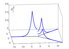
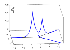
Figure 2: Two possible solutions are plotted. Here, $\beta_{1}=2/3$, $\beta_{2}=1$, and $\beta_{3}=2$ satisfying the condition for conserved norm and energy, and $\mu=0.1$. The solution in panel (a) is denoted by configuration $[1,1,1]$ and in panel (b) by $[1,1,0]$.

For a single nonlinear bond we have the solution

$$\phi_{1}(x)=\left\{\begin{array}[]{ll}\frac{B}{\sqrt{\beta_{1}}}e^{\sqrt{2\mu}(x+c)}\,{\rm at}\,x<-c,\\ \frac{A}{\sqrt{\beta_{1}}}e^{-\sqrt{2\mu}(x+c)}\,{\rm at}\,0\geq x>-c,\end{array}\right.$$ (34)

$$\phi_{2,3}(x)=\frac{A}{\sqrt{\beta_{2,3}}}e^{-\sqrt{2\mu}(x+c)}\,{\rm at}\,x\geq 0.$$ (35)

From the continuity of $\phi_{1}(x)$ at $x=-c$ we have

$$B=A.$$

One can find $A$ from the expression for the norm given by Eq. (2) :

$$A=\sqrt{\frac{2N\sqrt{2\mu}}{\left(\frac{1}{\beta_{2}}+\frac{1}{\beta_{3}}-\frac{1}{\beta_{1}}\right)e^{-2\sqrt{2\mu}c}+\frac{2}{\beta_{1}}}}.$$

The above analytical solution is obtained under the assumption that the constraint (20) is satisfied. In the following, we solve Eq. (12) numerically both for the case when the constraint in Eq. (20) is fulfilled and broken. The point nonlinearity in Eq. (12) is represented by the Gaussian function with $c=3$ and $a=0.1$. In the following, we only limit ourselves with positive solutions.

In Fig. 2, we plot two possible solutions for the case when the sum rule given by Eq. (20) is fulfilled. The first panel shows a solution when all the bonds are excited by the delta nonlinearity, while in the second one (b), only the first and the second bonds have point-like excitations. Using the configuration in the limit $\mu\to\infty$ as our code, we represent solutions in panels (a) and (b) as $[1,1,1]$ and $[1,1,0]$, respectively.

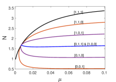
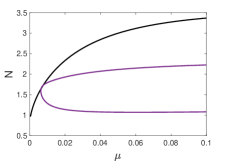
Figure 3: (a) Bifurcation diagram of solutions in Fig. 2. (b) The same diagram, but for $\beta_{j}=1$, $j=1,2,3.$

In Fig. 3, we present bifurcation diagrams of the solutions in Fig. 2. We obtain that the two configurations in Fig. 2 are connected with each other, with $[1,1,1]$ as the main branch and $[1,1,0]$ as a bifurcating solution through a pitchfork bifurcation with the configuration $[0,0,1]$. We therefore observe a spontaneous symmetry breaking bifurcation. It is particularly interesting to note that the bifurcation is quite degenerate in the sense that we obtain both a subcritical as well as a supercritical bifurcation emerging from the same point. We also obtain several other solutions bifurcating from the same bifurcation point, which are all indicated in Fig. 3.

We have considered a different case when all the nonlinearity coefficients are the same, i.e., without loss of nonlinearity $\beta_{j}=1$. In this case, the condition (20) is not satisfied. We plot the bifurcation diagram of the positive solutions in Fig. 3, where now we obtain that all the asymmetric solutions merge into two branches only, which bifurcate from the same point.

IV Conclusions

In this paper we obtained and analyzed exact solutions of NLSE on metric graphs with varying nonlinearity that has the form of a delta-well. Exact analytical solutions of the problem were obtained for different cases of point excitations, determined by the presence of a delta-well on different bonds. The constraint providing existence of such analytical solutions are derived in the form of simple sum, rule written in terms of the bond nonlinearity coefficients. Numerical solutions of the problem are also obtained both for integrable and non-integrable cases. Bifurcations of the solutions are studied in terms of chemical potential, using the numerical solutions $\mu$ using the numerical solutions. The model considered in this paper is relevant for different practically important problems such as BEC in branched traps, Bragg gratings in branched fibers, etc. Extension of the treatment to other graphs topologies is rather straightforward, provided the graphs contains arbitrary subgraph, which is connected to three or more outgoing semi-infinite bonds.

V Acknowledgements

This work is partially supported by a grant of the Ministry of Innovation Development of Uzbekistan (Ref. No. BF-2-022).

References

- (1) T. Kottos and U. Smilansky, Ann. Phys., 76 274 (1999).
- (2) P. Exner and H. Kovarik, Quantum waveguides. (Springer, 2015).
- (3) H. Susanto, S. van Gils, A. Doelman, and G. Derks, Physica C. 408, 579 (2004).
- (4) H. Susanto, S. van Gils, A. Doelman, and G. Derks, Phys. Rev. B 69, 212503 (2004).
- (5) T. Kottos and U. Smilansky, Ann. Phys., 76 274 (1999).
- (6) Z. Sobirov, D. Matrasulov, K. Sabirov, S. Sawada, and K. Nakamura, Phys. Rev. E 81 , 066602 (2010).
- (7) Z. Sobirov, D. Matrasulov, S. Sawada, and K. Nakamura, Phys.Rev.E 84, 026609 (2011).
- (8) R. Adami, C. Cacciapuoti, D. Finco, and D. Noja, Rev. Math. Phys. 23, 409 (2011).
- (9) R. Adami, C. Cacciapuoti, D. Finco, and D. Noja, Europhys. Lett. 100, 10003 (2012).
- (10) K.K.Sabirov, Z.A. Sobirov, D. Babajanov, and D.U. Matrasulov, Phys.Lett. A, 377, 860 (2013).
- (11) D. Noja, Philos. Trans. R. Soc. A 372, 20130002 (2014).
- (12) R. Adami, C. Cacciapuoti, D. Noja, J. Diff. Eq. 260, 7397 (2016).
- (13) J.-G Caputo , D. Dutykh, Phys. Rev. E 90, 022912 (2014).
- (14) H. Uecker, D. Grieser, Z. Sobirov, D. Babajanov and D. Matrasulov, Phys. Rev. E 91, 023209 (2015).
- (15) D. Noja, D. Pelinovsky, and G. Shaikhova, Nonlinearity 28, 2343 (2015)
- (16) Z. Sobirov, D. Babajanov, D. Matrasulov, K. Nakamura, and H. Uecker, EPL 115 , 50002 (2016).
- (17) A. Kairzhan, D.E. Pelinovsky, J. Phys. A: Math. Theor. 51, 095203 (2018).
- (18) K.K. Sabirov, S. Rakhmanov, D. Matrasulov and H. Susanto, Phys. Lett. A, 382, 1092 (2018).
- (19) K.K. Sabirov, D.B. Babajanov, D.U. Matrasulov and P.G. Kevrekidis, J. Phys. A: Math. Gen. 51 435203 (2018).
- (20) K.K. Sabirov, M. Akromov, Sh.R. Otajonov, D.U. Matrasulov, arXiv:1808.10751.
- (21) J. R. Yusupov, K. K. Sabirov, M. Ehrhardt, D. U. Matrasulov, ArXiv:1812.03736.
- (22) K.K. Sabirov, J. Yusupov, D. Jumanazarov, D. Matrasulov, Phys. Lett. A, 382, 2856 (2018).
- (23) D. Babajanov, H. Matyoqubov, D. Matrasulov, J. Chem. Phys., 149, 164908 (2018).
- (24) D. Noja, S. Rolando, S. Secchi, J. Diff. Eqn. 266, 147 (2019).
- (25) V. Kostrykin and R. Schrader J. Phys. A: Math. Gen. 32 595 (1999).
- (26) T. Mayteevarunyoo, B.A. Malomed, and G. Dong, Phys. Rev. A, 78, 053601 (2008).
- (27) V.A. Brazhnyi, B.A. Malomed, Phys. Rev. A, 83, 053844 (2011).
- (28) W. C. K. Mak, B. A. Malomed, and P. L. Chu, J. Opt. Soc. Am. B 15 1685 (1998).
- (29) A. Gubeskys and B. A. Malomed, Phys. Rev. A 75 063602 (2007).
- (30) M. Matuszewski, B. A. Malomed, and M. Trippenbach, Phys. Rev. A 75 063621 (2007).