Bounding the spectral gap for an elliptic eigenvalue problem with uniformly bounded stochastic coefficients

Abstract

A key quantity that occurs in the error analysis of several numerical methods for eigenvalue problems is the distance between the eigenvalue of interest and the next nearest eigenvalue. When we are interested in the smallest or fundamental eigenvalue, we call this the spectral or fundamental gap. In a recent manuscript [Gilbert et al., https://arxiv.org/abs/1808.02639], the current authors, together with Frances Kuo, studied an elliptic eigenvalue problem with homogeneous Dirichlet boundary conditions, and with coefficients that depend on an infinite number of uniformly distributed stochastic parameters. In this setting, the eigenvalues, and in turn the eigenvalue gap, also depend on the stochastic parameters. Hence, for a robust error analysis one needs to be able to bound the gap over all possible realisations of the parameters, and because the gap depends on infinitely-many random parameters, this is not trivial. This short note presents, in a simplified setting, an important result that was shown in the paper above. Namely, that, under certain decay assumptions on the coefficient, the spectral gap of such a random elliptic eigenvalue problem can be bounded away from 0, uniformly over the entire infinite-dimensional parameter space.

1 Introduction

Eigenvalue problems are useful for modelling many phenomena from applications in engineering and physics, e.g, structural mechanics, acoustic scattering, elastic membranes, criticality of neutron transport/diffusion and band gap calculations for photonic crystal fibres.

In this work, we consider the following eigenvalue problem

$$-\nabla\cdot\big{(}a({\bm{x}},{\bm{y}})\nabla u({\bm{x}},{\bm{y}})\big{)}\, =\,\lambda({\bm{y}})u({\bm{x}},{\bm{y}})\,,\quad \text{for }{\bm{x}}\in D,$$ (1.1)

$$u({\bm{x}},{\bm{y}})\, =\,0\,,\quad \text{for }{\bm{x}}\in\partial D\,,$$

where the derivatives are taken with respect to ${\bm{x}}$, and ${\bm{y}}=(y_{1},y_{2},\ldots)$ is a random, infinite-dimensional vector with independent uniformly distributed components $y_{j}\sim\mathrm{U}([-\tfrac{1}{2},\tfrac{1}{2}])$. We assume that the physical domain $D\subset\mathbb{R}^{d}$, for $d=1,2,3$, is bounded with Lipschitz boundary, and denote the stochastic/parameter domain by $U\coloneqq[-\tfrac{1}{2},\tfrac{1}{2}]^{\mathbb{N}}$.

In many uncertainty quantification (UQ) applications, the coefficient $a({\bm{x}},{\bm{y}})$ is given by a Karhunen–Loève expansion of a random field. Taking this as motivation, we assume that the coefficient is an affine map of ${\bm{y}}$, and satisfies

$$0\,<\,a({\bm{x}},{\bm{y}})\,=\,a_{0}({\bm{x}})+\sum_{j=1}^{\infty}y_{j}a_{j}({\bm{x}})\,<\,\infty\,,\quad\text{for all }x\in D,\ {\bm{y}}\in U.$$

Further assumptions on the coefficient will be given explicitly in Assumption A1 below.

If we ignore the ${\bm{y}}$ dependence, then (1.1) is a self-adjoint eigenvalue problem, which has been studied extensively in the literature, see, e.g., [7, 9]. In particular, it is well known that (1.1) has countably many eigenvalues

$$0\,<\,\lambda_{1}\,<\,\lambda_{2}\,\leq\,\lambda_{3}\,\leq\,\cdots\,,$$

and that the smallest eigenvalue is simple. However, in our setting the eigenvalues depend on ${\bm{y}}$: $\lambda_{k}=\lambda_{k}({\bm{y}})$, and since the parameter domain is infinite-dimensional, care must be taken when transferring classical results to our setting. In particular, although it is well known that in the unparametrised setting the spectral gap, $\lambda_{2}-\lambda_{1}$, is some fixed positive number, in our setting the spectral gap, $\lambda_{2}({\bm{y}})-\lambda_{1}({\bm{y}})$, is a function defined on an infinite-dimensional domain, which could be arbitrarily close to 0.

Our main result (see Theorem 3 for a full statement) is as follows. Assuming that the terms $a_{j}$ in the coefficient decay sufficiently fast (in a suitable norm), then there exists a $\delta>0$, independent of ${\bm{y}}$, such that the spectral gap of the eigenvalue problem (1.1) satisfies

$$\lambda_{2}({\bm{y}})-\lambda_{1}({\bm{y}})\,\geq\,\delta\,,\quad\text{for all }{\bm{y}}\in U\,.$$

As an example of the important role that the spectral gap plays in error analysis, consider the random elliptic eigenvalue problem from [8]. There, an algorithm using dimension truncation, Quasi–Monte Carlo (QMC) quadrature and finite element (FE) methods was used to approximate the expectation with respect to the stochastic parameters of the smallest eigenvalue. Throughout the error analysis the reciprocal of the spectral gap occurred in: 1) the bounds on the derivatives of the eigenvalues with respect to ${\bm{y}}$ (required for the QMC and dimension truncation error analysis); 2) the constants for the FE error; and 3) the convergence rate for the eigensolver (by Arnoldi iteration). In short, the entire error analysis in [8] fails unless the gap can be bounded from below uniformly in ${\bm{y}}$.

In the remainder of this section we frame (1.1) as a variational eigenvalue problem, introduce the function space setting and summarise some known properties of the eigenvalues. Then, in Section 2 we prove that the spectral gap is uniformly bounded. Finally, in Section 3 we perform a numerical experiment for a specific example of (1.1), and present results on the size of the gap over different realisations of the parameter generated by a QMC pointset.

1.1 Variational eigenvalue problems

It is often useful to study the eigenvalue problem (1.1) in its equivalent variational form. In this section we introduce the variational eigenvalue problem, then present some well known properties and tools that are required for our analysis.

First, we clarify the assumptions on the coefficient $a$ and our setting.

Assumption A 1.

1. The coefficient is of the form

   $$a({\bm{x}},{\bm{y}})\,=\,a_{0}({\bm{x}})+\sum_{j=1}^{\infty}y_{j}a_{j}({\bm{x}})\,,$$ (1.2)

   with $a_{j}\in L^{\infty}(D)$, for all $j\geq 0$.

2. There exists $0<a_{\min}<a_{\max}<\infty$ such that $a_{\min}\leq a({\bm{x}},{\bm{y}})\leq a_{\max}$, for all ${\bm{x}}\in D$, ${\bm{y}}\in U$.

3. For some $p\in(0,1)$,

   $$\sum_{j=1}^{\infty}\|a_{j}\|_{L^{\infty}}^{p}\,<\,\infty.$$

The last condition (Assumption 1.3) is the same as is required for the QMC and dimension truncation analysis for corresponding source problems (see [11]). Note that in that paper they also allow $p=1$, but with an extra condition on the size of the sum.

Also, the assumption from the Introduction that each $y_{j}$ is uniformly distributed is not a restriction, the important point is that each $y_{j}$ belongs to a bounded interval.

Let $V=H^{1}_{0}(D)$ equipped with the norm $\|v\|_{V}\coloneqq\|\nabla v\|_{L^{2}}$, and let $V^{*}$ denote the dual of $V$. We identify $L^{2}(D)$ with its dual, and denote the inner product on $L^{2}(D)$ by $\langle\cdot,\cdot\rangle$, which can be continuously extended to a duality pairing on $V\times V^{*}$, also denoted $\langle\cdot,\cdot\rangle$. Note that we have the following chain of compact embeddings $V\subset\subset L^{2}(D)\subset\subset V^{*}$. The parameter domain $U$ is equipped with the topology and metric of $\ell_{\infty}$.

Next, define the (parametric) symmetric bilinear form $\altmathcal{A}:U\times V\times V\to\mathbb{R}$ by

$$\altmathcal{A}({\bm{y}};w,v)\,\coloneqq\,\int_{D}a({\bm{x}},{\bm{y}})\nabla w({\bm{x}})\cdot\nabla v({\bm{x}})\,\,\mathrm{d}{\bm{x}}\,,$$

which is also an inner product on $V$.

In this setting, for each ${\bm{y}}\in U$, the variational eigenvalue problem equivalent to (1.1) is: Find $0\neq u({\bm{y}})\in V$ and $\lambda({\bm{y}})\in\mathbb{R}$ such that

$$\altmathcal{A}({\bm{y}};u({\bm{y}}),v) \,=\,\lambda({\bm{y}})\langle u({\bm{y}}),v\rangle,\quad\text{for all }v\in V\,,$$ (1.3)

$$\|u({\bm{y}})\|_{L^{2}} \,=\,1\,.$$

It follows from Assumption A1 that the bilinear form $\altmathcal{A}({\bm{y}})$ is coercive and bounded, uniformly in ${\bm{y}}$:

$$\altmathcal{A}({\bm{y}};v,v)\, \geq\,a_{\min}\|v\|_{V}^{2}\,,\quad \text{for all }v\in V\,,$$ and (1.4)

$$\altmathcal{A}({\bm{y}};w,v)\, \leq\,a_{\max}\|w\|_{V}\|v\|_{V}\,,\quad \text{for all }w,v\in V\,.$$ (1.5)

As a consequence, for each ${\bm{y}}$ we have a self-adjoint and coercive eigenvalue problem. Therefore, it is well known (see, e.g., [3, 9]) that (1.3) has a countable sequence of positive, real eigenvalues, which (counting multiplicities) we write as

$$0\,<\,\lambda_{1}({\bm{y}})\,\leq\,\lambda_{2}({\bm{y}})\,\leq\,\cdots\,,$$

and the corresponding eigenvectors are denoted by $u_{1}({\bm{y}}),u_{2}({\bm{y}}),\ldots\in V$.

The min-max principle [3, (8.36)]

$$\lambda_{k}({\bm{y}})\,=\,\min_{\begin{subarray}{c}V_{k}\subset V\\ \dim(V_{k})=k\end{subarray}}\max_{v\in V_{k}}\frac{\altmathcal{A}({\bm{y}};v,v)}{\langle v,v\rangle}\,,$$

allows us to bound each eigenvalue above and below independently of ${\bm{y}}$. Indeed, by (1.4) and (1.5) we have

$$a_{\min}\min_{\begin{subarray}{c}V_{k}\subset V\\ \dim(V_{k})=k\end{subarray}}\max_{v\in V_{k}}\frac{\langle\nabla v,\nabla v\rangle}{\langle v,v\rangle}\,\leq\,\lambda_{k}({\bm{y}})\,\leq\,a_{\max}\min_{\begin{subarray}{c}V_{k}\subset V\\ \dim(V_{k})=k\end{subarray}}\max_{v\in V_{k}}\frac{\langle\nabla v,\nabla v\rangle}{\langle v,v\rangle}\,.$$

Now, using the min-max properties of the $k$th eigenvalue of the Dirichlet Laplacian on $D$, which we denote by $\chi_{k}$, the bounds above simplify to

$$a_{\min}\chi_{k}\,\leq\,\lambda_{k}({\bm{y}})\,\leq\,a_{\max}\chi_{k}\,.$$ (1.6)

To consider our problem in the framework of Kato [10] for perturbations of linear operators, we introduce, for each ${\bm{y}}\in U$, the solution operator $T({\bm{y}}):V^{*}\rightarrow V$, which for $f\in V^{*}$ is defined by

$$\altmathcal{A}({\bm{y}};T({\bm{y}})f,v)\,=\,\langle f,v\rangle\quad\text{for all }v\in V\,.$$ (1.7)

Clearly, $\mu=1/\lambda$ is an eigenvalue of $T({\bm{y}})$ if and only if $\lambda$ is an eigenvalue of (1.3), and their eigenspaces coincide. Alternatively, we can consider the operator $T({\bm{y}}):L^{2}(D)\to L^{2}(D)$. In this case, $T({\bm{y}})$ is self-adjoint with respect to the $L^{2}$ inner product due to the symmetry of $\altmathcal{A}({\bm{y}})$; it is compact because $V\subset\subset L^{2}(D)$; and finally, it is bounded due to the Lax-Milgram theorem, which states that for each $f\in L^{2}(D)$ there is a unique $T({\bm{y}})f\in V$ satisfying (1.7), with

$$\|T({\bm{y}})f\|_{V}\,\leq\,\frac{1}{a_{\min}}\|f\|_{V^{*}}\,\leq\,\frac{1}{a_{\min}\sqrt{\chi_{1}}}\|f\|_{L^{2}}\,.$$ (1.8)

In the last inequality, we have used the Poincaré inequality:

$$\|v\|_{L^{2}}\,\leq\,\chi_{1}^{-1/2}\|v\|_{V}\,,\quad\text{for }v\in V\,,$$ (1.9)

and a standard duality argument. Note that we have expressed the Poincaré constant in terms of the smallest eigenvalue of the Dirichlet Laplacian on $D$, using again the min-max principle.

2 Bounding the spectral gap

The Krein-Rutman theorem guarantees that for every ${\bm{y}}$ the fundamental eigenvalue $\lambda_{1}({\bm{y}})$ is simple, see, e.g., [9, Theorems 1.2.5 and 1.2.6]. However, it does not provide any quantitative statements about the size of the spectral gap, $\lambda_{2}({\bm{y}})-\lambda_{1}({\bm{y}})$, for different parameter values ${\bm{y}}$. As discussed in the Introduction, when studying numerical methods for eigenvalue problems in a UQ setting (see, e.g., [8]) several areas of the error analysis require uniform positivity of this gap over all ${\bm{y}}\in U$. Here, we prove the required uniform positivity under the conditions of Assumption A1, in particular A1.3.

An explicit bound on the spectral gap can be obtained in slightly different settings or by assuming tighter restrictions on the coefficients. For example, for Schrödinger operators ($-\Delta+\mathcal{V}$) on $D$ with a weakly convex potential $\mathcal{V}$ and Dirichlet boundary conditions, [2] gives an explicit lower bound on the fundamental gap. Alternatively, using the upper and lower bounds on the eigenvalues (1.6), we can determine restrictions on $a_{\min}$ and $a_{\max}$ such that the gap is bounded away from 0. Explicitly, if the coefficient $a$ is such that $a_{\min}$ and $a_{\max}$ satisfy

$$\frac{a_{\min}}{a_{\max}}\,>\,\frac{\chi_{1}}{\chi_{2}}\,,$$ (2.1)

then, by (1.6), $\lambda_{2}({\bm{y}})-\lambda_{1}({\bm{y}})\geq a_{\min}\chi_{2}-a_{\max}\chi_{1}>0$. However, the condition (2.1) may prove to be too restrictive.

The general idea of our proof is to use the continuity of the eigenvalues to show that a non-zero minimum of the gap exists. A complication that arises in this strategy is that the parameter domain $U$ is not compact, so we cannot immediately conclude the existence of such a minumum; we know that $U$ cannot be compact in the topology of $\ell_{\infty}$ because it is the unit ball of $\ell_{\infty}$, and the unit ball of an infinite-dimensional Banach space is not compact. Our solution is based on the fact that although there are infinitely-many parameters, because of the decay of the terms in the coefficient (see Assumption A1.3), the contribution of a parameter $y_{j}$ decreases as $j$ increases. Specifically, we reparametrise (1.3) as an equivalent eigenvalue problem whose parameters do belong to a compact set.

The first step is the following elementary lemma, which shows that subsets of $\ell^{\infty}$ that are majorised by an $\ell^{q}$ sequence (for some $1<q<\infty$) are compact.

Lemma 1.

Let ${\bm{\alpha}}\in\ell^{q}$ for some $1<q<\infty$. The set $U({\bm{\alpha}})\subset\ell^{\infty}$ given by

$$U({\bm{\alpha}})\,\coloneqq\,\left\{{\bm{w}}\in\ell^{\infty}:|w_{j}|\leq\frac{1}{2}|\alpha_{j}|\right\}$$

is a compact subset of $\ell^{\infty}$.

Proof.

Since $\ell^{\infty}$ is a normed (and hence a metric) space, $U({\bm{\alpha}})$ is compact if and only if it is sequentially compact. To show sequential compactness of $U({\bm{\alpha}})$, take any sequence $\{{\bm{y}}^{(n)}\}_{n\geq 1}\subset U({\bm{\alpha}})$. Clearly, by definition of $U({\bm{\alpha}})$, each ${\bm{y}}^{(n)}\in\ell^{q}$ and moreover,

$$\|{\bm{y}}^{(n)}\|_{\ell^{q}}\,\leq\,\frac{1}{2}\|{\bm{\alpha}}\|_{\ell^{q}}\,<\,\infty\quad\text{for all }n\in\mathbb{N}\,.$$

So ${\bm{y}}^{(n)}$ is a bounded sequence in $\ell^{q}$. Since $q<\infty$, $\ell^{q}$ is a reflexive Banach space, and so by [4, Theorem 3.18] $\{{\bm{y}}^{(n)}\}_{n\geq 1}$ has a subsequence that converges weakly to a limit in $\ell^{q}$. We denote this limit by ${\bm{y}}^{*}$, and, with a slight abuse of notation, we denote the convergent subsequence again by $\{{\bm{y}}^{(n)}\}_{n\geq 1}$.

We now prove that ${\bm{y}}^{*}\in U({\bm{\alpha}})$ and that the weak convergence is in fact strong, i.e. we show ${\bm{y}}^{(n)}\rightarrow{\bm{y}}^{*}$ in $\ell^{\infty}$, as $n\rightarrow\infty$. For any $j\in\mathbb{N}$, consider the linear functional $f_{j}:\ell^{q}\rightarrow\mathbb{R}$ given by $f_{j}({\bm{w}})=w_{j}$, where $w_{j}$ denotes the $j$th element of the sequence ${\bm{w}}=(w_{j})_{j\geq 1}\in\ell^{q}$. Clearly, $f_{j}\in(\ell^{q})^{*}$ (the dual space) and using the weak convergence established above, it follows that

$$y_{j}^{(n)}\,=\,f_{j}({\bm{y}}^{(n)})\,\rightarrow\,f_{j}({\bm{y}}^{*})\,=\,y^{*}_{j}\quad\text{as }n\rightarrow\infty\,,\quad\text{for each fixed}\ \ j.$$

That is, we have componentwise convergence. Furthermore, since $|y_{j}^{(n)}|\leq\frac{1}{2}|\alpha_{j}|$ it follows that $|y_{j}^{*}|\leq\frac{1}{2}|\alpha_{j}|$ for each $j$, and hence ${\bm{y}}^{*}\in U({\bm{\alpha}})$.

Now, for any $J\in\mathbb{N}$ we can write

$$\|{\bm{y}}^{(n)}-{\bm{y}}^{*}\|_{\ell^{q}}^{q}\, =\,\sum_{j=1}^{J}|y_{j}^{(n)}-y_{j}^{*}|^{q}+\sum_{j=J+1}^{\infty}|y_{j}^{(n)}-y_{j}^{*}|^{q}$$

$$\leq\,J\max_{j=1,2,\ldots,J}|y_{j}^{(n)}-y_{j}^{*}|^{q}+\sum_{j=J+1}^{\infty}|\alpha_{j}|^{q}\,.$$ (2.2)

Let $\varepsilon>0$. Since ${\bm{\alpha}}\in\ell^{q}$, we can choose $J\in\mathbb{N}$ such that

$$\sum_{j=J+1}^{\infty}|{\alpha_{j}}|^{q}\,\leq\,\frac{\varepsilon^{q}}{2}\,,$$

and since ${\bm{y}}^{(n)}$ converges componentwise we can choose $K\in\mathbb{N}$ such that

$$|y_{j}^{(n)}-y_{j}^{*}|\,\leq\,(2J)^{-1/q}\varepsilon\quad\text{for all }j=1,2,\ldots,J\text{ and }n\geq K\,.$$

Thus, by (2) we have $\|{\bm{y}}^{(n)}-{\bm{y}}^{*}\|_{\ell^{q}}^{q}\leq\varepsilon^{q}$ for all $n\geq K$, and hence $\|{\bm{y}}^{(n)}-{\bm{y}}^{*}\|_{\ell^{q}}\rightarrow 0$ as $n\rightarrow\infty$. Because $\|{\bm{w}}\|_{\ell^{\infty}}\leq\|{\bm{w}}\|_{\ell^{q}}$ when ${\bm{w}}\in\ell^{q}$ and $1<q<\infty$, this also implies that ${\bm{y}}^{(n)}\rightarrow{\bm{y}}^{*}$ in $\ell^{\infty}$, completing the proof. ∎

A key property following from the perturbation theory of Kato [10] is that the eigenvalues $\lambda_{k}({\bm{y}})$ are continuous in ${\bm{y}}$, which for completeness is shown below in Proposition 2. First, recall that $T({\bm{y}})$ is the solution operator as defined in (1.7), and let $\Sigma(T({\bm{y}}))$ denote the spectrum of $T({\bm{y}})$.

Proposition 2.

Let Assumption A1 hold. Then the eigenvalues $\lambda_{1},\lambda_{2},\ldots$ are Lipschitz continuous in ${\bm{y}}$.

Proof.

We prove the result by establishing the continuity of the eigenvalues $\mu_{k}({\bm{y}})$ of $T({\bm{y}})$. Let ${\bm{y}}$, ${\bm{y}}^{\prime}\in U$ and consider the operators $T({\bm{y}}),T({\bm{y}}^{\prime}):L^{2}(D)\rightarrow L^{2}(D)$ as defined in (1.7). Since $T({\bm{y}})$, $T({\bm{y}}^{\prime})$ are bounded and self-adjoint with respect to $\langle\cdot,\cdot\rangle$, it follows from [10, V, §4.3 and Theorem 4.10] that we have the following notion of continuity of $\mu(\cdot)$ in terms of $T(\cdot)$

$$\sup_{\mu\in\Sigma(T({\bm{y}}))}\mathrm{dist}(\mu,\Sigma(T({\bm{y}}^{\prime})))\,\leq\,\|T({\bm{y}})-T({\bm{y}}^{\prime})\|_{L^{2}\rightarrow L^{2}}\,.$$ (2.3)

For an eigenvalue $\mu_{k}({\bm{y}})\in\Sigma(T({\bm{y}}))$, (2.3) implies that there exists a $\mu_{k^{\prime}}({\bm{y}}^{\prime})\in\Sigma(T({\bm{y}}^{\prime}))$ such that

$$|\mu_{k}({\bm{y}})-\mu_{k^{\prime}}({\bm{y}}^{\prime})|\,\leq\,\|T({\bm{y}})-T({\bm{y}}^{\prime})\|_{L^{2}\rightarrow L^{2}}\,.$$ (2.4)

Note that this means there exists an eigenvalue of $T({\bm{y}}^{\prime})$ close to $\mu_{k}({\bm{y}})$, but does not imply that the $k$th eigenvalue of $T({\bm{y}}^{\prime})$ is close to $\mu_{k}({\bm{y}})$, that is, in (2.4) $k$ is not necessarily equal to $k^{\prime}$. However, consider any $\mu_{k}({\bm{y}})$ and let $m$ denote its multiplicity. Since $m<\infty$, we can assume without loss of generality that the collection $\mu_{k}({\bm{y}})=\mu_{k+1}({\bm{y}})=\cdots=\mu_{k+m-1}({\bm{y}})$ is a finite system of eigenvalues in the sense of Kato. It then follows from the discussion in [10, IV, §3.5] that the eigenvalues in this system depend continuously on the operator with multiplicity preserved. This preservation of multiplicity is key to our argument, since it states that for $T({\bm{y}}^{\prime})$ sufficiently close to $T({\bm{y}})$ there are $m$ consecutive eigenvalues $\mu_{k^{\prime}}({\bm{y}}^{\prime}),\mu_{k^{\prime}+1}({\bm{y}}^{\prime}),\ldots,\mu_{k^{\prime}+m-1}({\bm{y}}^{\prime})\in\Sigma(T({\bm{y}}^{\prime}))$, no longer necessarily equal, that are close to $\mu_{k}({\bm{y}})$.

A simple argument then shows that each $\mu_{k}$ is continuous in the following sense

$$|\mu_{k}({\bm{y}})-\mu_{k}({\bm{y}}^{\prime})|\,\leq\,\|T({\bm{y}})-T({\bm{y}}^{\prime})\|_{L^{2}\rightarrow L^{2}}\,.$$ (2.5)

To see this, consider, for $k=1,2,\ldots$, the graphs of $\mu_{k}$ on $U$. Note that the separate graphs can touch (and in principle can even coincide over some subset of $U$), but by definition cannot cross (since at every point in $U$ the successive eigenvalues are nonincreasing); and by the preservation of multiplicity a graph cannot terminate and a finite set of graphs cannot change multiplicity at an interior point. Thus by (2.23) the ordered eigenvalues $\mu_{k}$ must be continuous for each $k\geq 1$ and satisfy (2.5).

It then follows from the relationship $\mu_{k}({\bm{y}})=1/\lambda_{k}({\bm{y}})$ along with the upper bound in (1.6) that we have a similar result for the eigenvalues $\lambda_{k}$ of (1.3):

$$\left|\lambda_{k}({\bm{y}})-\lambda_{k}({\bm{y}}^{\prime})\right|\,\leq\,(a_{\max}\chi_{k})^{2}\|T({\bm{y}})-T({\bm{y}}^{\prime})\|_{L^{2}\rightarrow L^{2}}\,.$$ (2.6)

All that remains is to bound the right hand side of (2.6) by $C_{\mathrm{Lip}}\|{\bm{y}}-{\bm{y}}^{\prime}\|_{\ell^{\infty}}$, with $C_{\mathrm{Lip}}>0$ independent of ${\bm{y}}$ and ${\bm{y}}^{\prime}$. To this end, note that since the right hand side of (1.7) is independent of ${\bm{y}}$ we have

$$\altmathcal{A}({\bm{y}};T({\bm{y}})f,v)\,=\,\altmathcal{A}({\bm{y}}^{\prime};T({\bm{y}}^{\prime})f,v)\quad\text{for all }f\in L^{2}(D),v\in V\,.$$

Rearranging and then expanding this gives

$$\altmathcal{A}\left({\bm{y}};\left(T({\bm{y}})-T({\bm{y}}^{\prime})\right)f,v\right))\, =\,\altmathcal{A}({\bm{y}}^{\prime};T({\bm{y}}^{\prime})f,v)-\altmathcal{A}({\bm{y}};T({\bm{y}}^{\prime})f,v)$$

$$=\,\int_{D}\left[a({\bm{x}},{\bm{y}}^{\prime})-a({\bm{x}},{\bm{y}})\right]\nabla[T({\bm{y}}^{\prime})f]({\bm{x}})\cdot\nabla v({\bm{x}})\,\,\mathrm{d}{\bm{x}}\,.$$

Letting $v=(T({\bm{y}})-T({\bm{y}}^{\prime}))f\in V$, the left hand side can be bounded from below using the coercivity (1.4) of $\altmathcal{A}({\bm{y}})$, and the right hand side can be bounded from above using the Cauchy-Schwarz inequality to give

$$a_{\min}\|(T({\bm{y}})-T({\bm{y}}^{\prime}))f\|_{V}^{2}\,\leq\,\|a({\bm{y}})-a({\bm{y}}^{\prime})\|_{L^{\infty}}\|T({\bm{y}}^{\prime})f\|_{V}\|(T({\bm{y}})-T({\bm{y}}^{\prime}))f\|_{V}\,.$$

Dividing by $a_{\min}\|(T({\bm{y}})-T({\bm{y}}^{\prime}))f\|_{V}$ and using the upper bound in (1.8) we have

$$\|(T({\bm{y}})-T({\bm{y}}^{\prime}))f\|_{V}\,\leq\,\frac{1}{a_{\min}^{2}\sqrt{\chi_{1}}}\|f\|_{L^{2}}\|a({\bm{y}})-a({\bm{y}}^{\prime})\|_{L^{\infty}}\,.$$

Then, applying the Poincaré inequality (1.9) to the left hand side and taking the supremum over $f\in L^{2}(D)$ with $\|f\|_{L^{2}}\leq 1$, in the operator norm we have

$$\|T({\bm{y}})-T({\bm{y}}^{\prime})\|_{L^{2}\rightarrow L^{2}}\,\leq\,\frac{1}{a_{\min}^{2}\chi_{1}}\|a({\bm{y}})-a({\bm{y}}^{\prime})\|_{L^{\infty}}\,.$$

Using this inequality as an upper bound for (2.6) we see that the eigenvalues inherit the continuity of the coefficient, and so

$$|\lambda_{k}({\bm{y}})-\lambda_{k}({\bm{y}}^{\prime})|\,\leq\,\frac{a_{\max}^{2}\chi_{k}^{2}}{a_{\min}^{2}\chi_{1}}\|a({\bm{y}})-a({\bm{y}}^{\prime})\|_{L^{\infty}}\,.$$ (2.7)

where the constant is clearly independent of ${\bm{y}}$ and ${\bm{y}}^{\prime}$.

Finally, to establish Lipschitz continuity with respect to ${\bm{y}}$, we recall Assumptions A1.1 and A1.3, expand the coefficients in (2.7) above and use the triangle inequality to give

$$|\lambda_{k}({\bm{y}})-\lambda_{k}({\bm{y}}^{\prime})|\,\leq\,\frac{a_{\max}^{2}\chi_{k}^{2}}{a_{\min}^{2}\chi_{1}}\sum_{j=1}^{\infty}|y_{j}-y_{j}^{\prime}|\|a_{j}\|_{L^{\infty}}\,\leq\,\frac{a_{\max}^{2}\chi_{k}^{2}}{a_{\min}^{2}\chi_{1}}\Bigg{(}\sum_{j=1}^{\infty}\|a_{j}\|_{L^{\infty}}\Bigg{)}\|{\bm{y}}-{\bm{y}}^{\prime}\|_{\ell^{\infty}}\,.$$

By Assumption 1 the sum is finite, and hence the eigenvalue $\lambda_{k}({\bm{y}})$ is Lipschitz in ${\bm{y}}$, with the constant clearly independent of ${\bm{y}}$. ∎

Now that we have shown Lipschitz continuity of the eigenvalues and identified suitable compact subsets, we can prove the main result of this paper: namely, that the spectral gap is bounded away from 0 uniformly in ${\bm{y}}$. The strategy of the proof is to rewrite the coefficient as

$$a({\bm{x}},{\bm{y}})\ =\ a_{0}({\bm{x}})\ +\ \sum_{j=1}^{\infty}\widetilde{y}_{j}\widetilde{a}_{j}({\bm{x}})\,,$$

with $\widetilde{y}_{j}=\alpha_{j}y_{j}$ and $\widetilde{a}_{j}({\bm{x}})=a_{j}({\bm{x}})/\alpha_{j}$, choosing ${\bm{\alpha}}\in\ell^{q}$ to decay slowly enough such that $\sum_{j=1}^{\infty}\|\widetilde{a}_{j}\|_{L^{\infty}}<\infty$ continues to hold. Then, using the intermediate result (2.7) from the proof of Proposition 2 we can show that the eigenvalues of the “reparametrised” problem are continuous in the new parameter $\widetilde{\bm{y}}$, which now ranges over the compact set $U({\bm{\alpha}})$. The required bound on the spectral gap is obtained by using the equivalence of the eigenvalues of the original and reparametrised problems.

Theorem 3.

Let Assumption A1 hold. Then there exists a $\delta>0$, independent of ${\bm{y}}$, such that

$$\lambda_{2}({\bm{y}})-\lambda_{1}({\bm{y}})\,\geq\,\delta\,.$$ (2.8)

Proof.

We can assume, without loss of generality, that $p>1/2$, because if Assumption A1.3 holds with exponent $p^{\prime}\leq 1/2$ then it also holds for all $p\in(p^{\prime},1)$. Consequently, set $\varepsilon=1-p\in(0,1/2)$ and consider the sequence ${\bm{\alpha}}$ defined by

$$\alpha_{j}\,=\,\|a_{j}\|^{\varepsilon}_{L^{\infty}}+1/j,\quad\text{for each}\ \ j\in\mathbb{N}.$$ (2.9)

Setting $q=p/\varepsilon=p/(1-p)\in(1,\infty)$, using Assumption A1.3 and the triangle inequality, it is easy to see that ${\bm{\alpha}}\in\ell^{q}$. Moreover, the inclusion of $1/j$ in (2.9) ensures that $\alpha_{j}\not=0$, for all $j\geq 1$. Hence, from now on, for ${\bm{w}}=(w_{j})_{j=1}^{\infty}\in\ell^{\infty}$, we can define the sequences ${\bm{\alpha}}{\bm{w}}=(\alpha_{j}w_{j})_{j=1}^{\infty}$ and ${\bm{w}}/{\bm{\alpha}}=(w_{j}/\alpha_{j})_{j=1}^{\infty}$. Then, recalling the definition of $U({\bm{\alpha}})$ in Lemma 1, it is easy to see that$\widetilde{\bm{y}}\in U({\bm{\alpha}})$ if and only if $\widetilde{\bm{y}}/{\bm{\alpha}}\in U$, and moreover, ${\bm{y}}\in U$ if and only if ${\bm{\alpha}}{\bm{y}}\in U({\bm{\alpha}})$.

Now for ${\bm{x}}\in D$ and $\widetilde{\bm{y}}\in U({\bm{\alpha}})$, we define

$$\widetilde{a}({\bm{x}},\widetilde{\bm{y}})=a_{0}({\bm{x}})+\sum_{j=1}^{\infty}\widetilde{y}_{j}\frac{a_{j}({\bm{x}})}{\alpha_{j}}\,,$$

from which it is easily seen that

$$\widetilde{a}({\bm{x}},\widetilde{\bm{y}})=a({\bm{x}},\widetilde{\bm{y}}/{\bm{\alpha}})\,.$$ (2.10)

Then we set

$$\widetilde{\altmathcal{A}}(\widetilde{{\bm{y}}};w,v)\,\coloneqq\,\int_{D}\widetilde{a}({\bm{x}},\widetilde{{\bm{y}}})\nabla w({\bm{x}}).\nabla v({\bm{x}})\,\,\mathrm{d}{\bm{x}}\quad\text{for }w,v\in V\,,$$

and we consider the following reparametrised eigenvalue problem: Find $\widetilde{\lambda}(\widetilde{{\bm{y}}})\in\mathbb{R}$ and $0\neq\widetilde{u}(\widetilde{{\bm{y}}})\in V$ such that

$$\widetilde{\altmathcal{A}}(\widetilde{{\bm{y}}};\widetilde{u}(\widetilde{{\bm{y}}}),v)\, =\,\widetilde{\lambda}_{k}(\widetilde{{\bm{y}}})\langle\widetilde{u}(\widetilde{{\bm{y}}}),v\rangle\quad\text{for all }v\in V\,,$$

$$\|\widetilde{u}(\widetilde{{\bm{y}}})\|_{L^{2}}\, =\,1\,.$$ (2.11)

Note that because we have equality between the original and reparametrised coefficients (2.10), for each ${\bm{y}}\in U$, and corresponding $\widetilde{\bm{y}}={\bm{\alpha}}{\bm{y}}\in U({\bm{\alpha}})$, (2.10) implies that there is equality between eigenvalues $\lambda_{k}({\bm{y}})$ of (1.3) and $\widetilde{\lambda}_{k}(\widetilde{\bm{y}})$ of the reparametrised eigenvalue problem (2)

$$\lambda_{k}({\bm{y}})\,=\,\widetilde{\lambda}_{k}(\widetilde{\bm{y}})\quad\text{for }k\in\mathbb{N}\,,$$ (2.12)

and their eigenspaces coincide.

Moreover, for an eigenvalue $\widetilde{\lambda}_{k}(\widetilde{\bm{y}})$ of (2), using (2.12) in the inequality (2.7) we have

$$|\widetilde{\lambda}_{k}(\widetilde{{\bm{y}}})-\widetilde{\lambda}_{k}(\widetilde{{\bm{y}}}^{\prime})|\,\leq\,\frac{a_{\max}^{2}\chi_{k}^{2}}{a_{\min}^{2}\chi_{1}}\|a(\widetilde{\bm{y}}/{\bm{\alpha}})-a(\widetilde{\bm{y}}/{\bm{\alpha}})\|_{L^{\infty}}\,,$$

which after expanding the coefficient and using the triangle inequality becomes

$$|\widetilde{\lambda}_{k}(\widetilde{{\bm{y}}})-\widetilde{\lambda}_{k}(\widetilde{{\bm{y}}}^{\prime})|\,\leq\,\Bigg{(}\underbrace{\frac{a_{\max}^{2}\chi_{k}^{2}}{a_{\min}^{2}\chi_{1}}\sum_{j=1}^{\infty}\frac{1}{\alpha_{j}}\|a_{j}\|_{L^{\infty}}}_{\widetilde{C}_{\mathrm{Lip}}}\Bigg{)}\|\widetilde{\bm{y}}-\widetilde{\bm{y}}^{\prime}\|_{\ell^{\infty}}\,,$$

where $\widetilde{C}_{\mathrm{Lip}}$ is clearly independent of $\widetilde{\bm{y}}$ and $\widetilde{\bm{y}}^{\prime}$. Now by (2.9) together with Assumption A1, we have

$$\sum_{j=1}^{\infty}\frac{\|a_{j}\|_{L^{\infty}}}{\alpha_{j}}\ \leq\ \sum_{j=1}^{\infty}\|a_{j}\|_{L^{\infty}}^{1-\varepsilon}\ =\ \sum_{j=1}^{\infty}\|a_{j}\|_{L^{\infty}}^{p}<\ \infty\,.$$

Thus, $\widetilde{C}_{\mathrm{Lip}}<\infty$ and hence the reparametrised eigenvalues are continuous on $U({\bm{\alpha}})$.

It immediately follows that the spectral gap $\widetilde{\lambda}_{2}(\widetilde{{\bm{y}}})-\widetilde{\lambda}_{1}(\widetilde{{\bm{y}}})$ is also continuous on $U({\bm{\alpha}})$, which by Lemma 1 is a compact subset of $\ell^{\infty}$. Therefore, the non-zero minimum is attained giving that the spectral gap $\widetilde{\lambda}_{2}(\widetilde{{\bm{y}}})-\widetilde{\lambda}_{1}(\widetilde{{\bm{y}}})$ is uniformly positive. Finally, because there is equality between the original and reparametrised eigenvalues (2.12) the result holds for the original problem over all ${\bm{y}}\in U$. ∎

The paper [8] proves a similar result to Theorem 3 in a more general setting, the same strategy is used there also.

3 Numerical results

For our numerical results, we consider the 1-dimensional domain $D=(0,1)$, and let the basis functions that define the coefficient in (1.2) be given by

$$a_{j}(x)\,=\,\begin{cases}a_{0}&\text{for }j=0,\\[5.69054pt] \displaystyle\frac{c_{0}}{j^{2}}\sin(j\pi x)\,,&\text{for }j=1,2,\ldots,s,\\[5.69054pt] 0&\text{for }j>s,\end{cases}$$ (3.1)

where $a_{0}>0$ and $c_{0}\in\mathbb{R}$ will determine the values of $a_{\min}$ and $a_{\max}$. Note that the stochastic dimension is here fixed at $s=100$. Since multiplying the coefficient by any constant factor will simply rescale the eigenvalues by that same factor, without loss of generality we can henceforth set $a_{0}=1$ and vary $c_{0}$.

For a coefficient (1.2) given by the basis functions (3.1), we can obtain a formula for the bounds $a_{\min}$, $a_{\max}$ as follows

$$a_{\min}\,=\,1-\frac{c_{0}}{2}\sum_{j=1}^{s}\frac{1}{j^{2}}\,=\,1-0.81c_{0}\,,$$

$$a_{\max}\,=\,1+\frac{c_{0}}{2}\sum_{j=1}^{s}\frac{1}{j^{2}}\,=\,1+0.81c_{0}\,.$$

We remark that these bounds are not sharp.

We also consider the so-called log-normal coefficient:

$$a(x,{\bm{y}})=a_{*}+\exp\Bigg{(}\sum_{j=1}^{s}\Phi^{-1}(y_{j}+\tfrac{1}{2})a_{j}(x)\Bigg{)}\,,$$ (3.2)

where $a_{*}\geq 0$, $a_{j}$ are as in (3.1), and $\Phi^{-1}$ is the inverse of the normal cumulative distribution function. In this way each $\Phi^{-1}(y_{j}+\tfrac{1}{2})\sim\altmathcal{N}(0,1)$. Since $\Phi^{-1}$ maps $[0,1]$ to $\mathbb{R}$, the coefficient (3.2) is unbounded, and although it is positive ($a_{\min}=a_{*}$), for $a_{*}=0$ it could be arbitrarily close to 0. So in this case Assumption 1.2 does not hold, our compactness argument fails and we have no theoretical prediction.

To approximate the eigenvalue problem in space we use piecewise linear finite elements on a uniform mesh, with a meshwidth of $h=1/64$. Numerical tests for different meshwidths ($h=1/8$ to $h=1/128$) produced qualitatively the same results.

The purpose of this section is to provide supporting evidence that for the problem above the gap remains bounded. We do this in a brute force manner by studying the minimum of the gap over a large number of parameter realisations. The parameter realisations are generated by a QMC point set; specifically, a base-2 embedded lattice rule (see [5]) with up to $2^{20}$ points and a single random shift. To generate the points we use the generating vector exod2_base2_m20_CKN from [12]. We choose QMC points as the test set because they can be shown to be well-distributed in high dimensions, see e.g. [5, 6]. The goal is not to find the minimum, but to provide evidence that as more and more of the parameter domain is searched (which corresponds to more realisations), the minimum of the gap over all realisations approaches a constant value.

The results are given in Figures 1–5, where in each figure we plot the minimum of the gap against the number of realisations $N$ (blue circles) and an estimate (see the next paragraph) of the distance between the estimated minimum and the true minimum (black triangles), along with a least-squares fit to $\alpha N^{-\beta}$ (dashed red line) of this estimate. Each data point corresponds to a doubling of the number of QMC points: $N=1,2,4,\ldots,2^{20}$, and the axes are in loglog scale.

Letting $\delta_{N}$ denote the approximate minimum over the first $N$ realisations, we estimate the distance to the true minimum by

$$\delta_{N}-\min_{{\bm{y}}\in U}\big{(}\lambda_{2}({\bm{y}})-\lambda_{1}({\bm{y}})\big{)}\,\approx\,\delta_{N}-\delta_{N^{*}}\,,$$

where $\delta_{N^{*}}$ corresponds to the most accurate estimate of the minimum, with $N^{*}=2^{20}$. The purpose of including such an estimate of the distance to the true minimum is to demonstrate that not only does the minimum of the gap appear to plateau, but that the differences also decay like a power of $N$.

First we consider the affine coefficient in (1.2). The three different choices of $c_{0}$ are: in Figure 1 $c_{0}=1$, which gives $a_{\min}=0.18$ and $a_{\max}=1.82$; in Figure 2 $c_{0}=1.223$, which gives $a_{\min}=2\times 10^{-4}$ and $a_{\max}=2$; and in Figure 3 $c_{0}=0.5$, which gives $a_{\min}=0.59$ and $a_{\max}=1.41$. Then, in Figure 4 we plot the log-normal coefficient (3.2) with $a_{\min}=a_{*}=0$ and $c_{0}=1$, and in Figure 5 we plot the lognormal coefficient with $a_{\min}=a_{*}=0.18$ and $c_{0}=1$.

For each different choice of the affine coefficient (1.2) (Figures 1, 2, 3), the minimum value of the gap appears to plateau and approach a nonzero minimum. The minimum of the gap seems fairly insensitive to changes in $c_{0}$. However, in Figures 4 and 5 for the log-normal coefficient (which, we recall is not covered by the theory of the current work) the results are inconclusive. It appears that the gap tends to 0 in the case of a true lognormal coefficient ($a_{*}=0$, Figure 4), and that it is bounded away from 0 for the “regularised” lognormal coefficient with $a_{*}=0.18$ in Figure 5. However, in Figure 4 the smallest computed value of the gap is close to 1, and it is possible that it will plateau for a denser set of QMC points. Also, in Figure 5 the plateau is not as clearly developed in as in Figures 1–3. It remains an open question if the gap can be bounded in the case of the lognormal coefficient (3.2), and whether $a_{*}$ needs to be strictly positive.

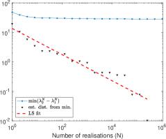
Figure 1: Estimate of the minimum of the spectral gap and estimate of the distance to the true minimum: affine coefficient (1.2) with $a_{0}=c_{0}=1$, $a_{\min}=0.18$, $a_{\max}=1.82$.

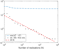
Figure 2: Estimate of the minimum of the spectral gap and estimate of the distance to the true minimum: affine coefficient (1.2) with $a_{0}=1$, $c_{0}=1.223$, $a_{\min}=2\times 10^{-4}$, $a_{\max}=2$.

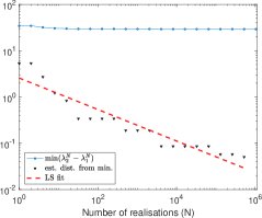
Figure 3: Estimate of the minimum of the spectral gap and estimate of the distance to the true minimum: affine coefficient (1.2) with $a_{0}=1$, $c_{0}=0.5$, $a_{\min}=0.59$, $a_{\max}=1.41$.

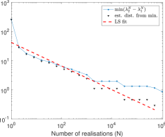
Figure 4: Estimate of the minimum of the spectral gap and estimate of the distance to the true minimum: log-normal coefficient (3.2) with $a_{\min}=a_{*}=0$ and $c_{0}=1$.

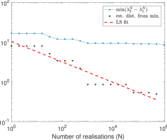
Figure 5: Estimate of the minimum of the spectral gap and estimate of the distance to the true minimum: log-normal coefficient (3.2) with $a_{\min}=a_{*}=0.18$ and $c_{0}=1$.

4 Conclusion

The spectral gap is an important quantity that occurs throughout several areas of the numerical analysis of eigenvalue problems, and in this work we proved that, under certain conditions on the coefficient, the spectral gap of a random elliptic eigenvalue problem is uniformly bounded from below. In all of our numerical experiments the results strongly suggest that the minimum of the gap approaches a nonzero constant value. The only exception is the lognormal coefficient, which is not covered by our theory.

References

- [1] R. Andreev and Ch. Schwab. Sparse tensor approximation of parametric eigenvalue problems. In I. G. Graham et al, editor, Numerical Analysis of Multiscale Problems, Lecture Notes in Computational Science and Engineering, 203–241. Springer-Verlag, Berlin Heidelberg, Germany, 2012.
- [2] B. Andrews and J. Clutterbuck. Proof of the fundamental gap conjecture. J. Amer. Math. Soc. 24, 899–916, 2011.
- [3] I. Babuška and J. Osborn. Eigenvalue problems. In P. G. Ciarlet and J. L. Lions, editors, Handbook of Numerical Analysis, Volume 2: Finite Element Methods (Part 1), 641–787. Elsevier Science, Amsterdam, The Netherlands, 1991.
- [4] H. Brezis, Functional Analysis, Sobolev Spaces and Partial Differential Equations. Universitext, Springer, New York, 2011.
- [5] R. Cools, F. Y. Kuo and D. Nuyens, Constructing embedded lattice rules for multivariate integration. SIAM J. Sci. Comp., 28, 2162–2188, 2006.
- [6] J. Dick, F. Y. Kuo, and I. H. Sloan. High-dimensional integration: The quasi-Monte Carlo way. Acta Numerica, 22, 133–288, 2013.
- [7] N. Dunford and J. T. Schwartz, Linear Operators, Part II: Spectral Theory, Self Adjoint Operators in Hilbert Space. Interscience Publishers, New York London, 1963.
- [8] A. D. Gilbert, I. G. Graham, F. Y. Kuo, R. Scheichl and I. H. Sloan, Analysis of quasi-Monte Carlo Methods for elliptic eigenvalue problems with stochastic coefficients. Submitted, arXiv: https://arxiv.org/abs/1808.02639, 2018.
- [9] A. Henrot. Extremum Problems for Eigenvalues of Elliptic Operators. Birkhäuser Verlag, Basel, Switzerland, 2006.
- [10] T. Kato. Perturbation Theory for Linear Operators. Springer-Verlag, Berlin Heidelberg, Germany, 1984.
- [11] F. Y. Kuo, Ch. Schwab, and I. H. Sloan. Quasi-Monte Carlo finite element methods for a class of elliptic partial differential equations with random coefficients. SIAM J. Numer. Anal., 50, 3351–3374, 2012.
- [12] D. Nuyens, https://people.cs.kuleuven.be/~dirk.nuyens/qmc-generators/, accessed November 2, 2018.