A Minimalistic Approach to Segregation
in Robot Swarms

Abstract

We present a decentralized algorithm to achieve segregation into an arbitrary number of groups with swarms of autonomous robots. The distinguishing feature of our approach is in the minimalistic assumptions on which it is based. Specifically, we assume that (i) Each robot is equipped with a ternary sensor capable of detecting the presence of a single nearby robot, and, if that robot is present, whether or not it belongs to the same group as the sensing robot; (ii) The robots move according to a differential drive model; and (iii) The structure of the control system is purely reactive, and it maps directly the sensor readings to the wheel speeds with a simple ‘if’ statement. We present a thorough analysis of the parameter space that enables this behavior to emerge, along with conditions for guaranteed convergence and a study of non-ideal aspects in the robot design.

I Introduction

Group formation is one of the most fundamental mechanisms a robot swarm must exhibit [1]. Group formation can occur in several forms to satisfy different requirements. Segregation is a particular type of group formation in which the focus is on creating local aggregates of robots that share a common property. Segregation can be seen as a precursor to object sorting, task allocation, or self-assembly. For example, swarms may need to split into arbitrary groups to diffuse and search different areas, or segregate by skill or capability in order to form useful heterogeneous teams.

Segregation is an example of the broader class of spatially organizing behaviors, whose purpose is to impose a structure in the environment (e.g., object clustering [2], collective construction [3]) or in the distribution of the robots (e.g., aggregation [4], pattern formation [5], self-assembly [6]).

A recent line of research in spatially organizing behaviors focuses on the minimal assumptions a swarm of robots must fulfill in order to perform the task. Johnson and Brown [7] and Brown et al. [8] characterized the set of possible behaviors that can be obtained using primordial control strategies based on a simple ‘if/then/else’ structure, binary sensors, and differential-drive robots. Gauci et al. provided the specific conditions for the emergence of aggregation [9] and object clustering [2], while St.-Onge et al. [10] studied the emergence of circular formations. While more efficient control strategies have been proposed to achieve these behaviors, studying the minimal assumptions required for their emergence is an important step towards principled ‘swarm engineering’ practices. In addition, these minimal behaviors might offer last-resort solutions in case of sensor failures in remote environments such as in planetary exploration missions.

This paper furthers this line of inquiry by studying the minimal assumptions for $N$-class segregation to emerge from local, decentralized interactions among robots. The term ‘$N$-class’ refers to the creation of $N$ spatially distinct groups. We show that, for segregation to emerge, it is sufficient to equip an ‘if/then/else’, differential drive robot with a ternary sensor. This sensor detects the presence of a robot in range. When a robot is detected, the sensor can distinguish whether it is a kin, i.e., it belongs to the same group as the sensing robot, or a non-kin, i.e., it belongs to a different group. When multiple robots are in range, the sensor returns information on the closest one of them.

The main contributions of this paper are (i) A study of the parameter space that enables the emergence of $N$-class segregation; (ii) A study of why convergence is guaranteed for the best parameter choice found; and (iii) An analysis of the robustness of the algorithm to non-idealities in the robot design.

II Related Work

Segregation is a common behavior in nature, and it can be observed across scales. For example, cell segregation is a basic building block of embryogeneis in tissue generation processes [11, 12]; while social insects, such as ants, organize their brood into ring-like structures [13].

In robotics, segregation is a problem that has not received considerable attention. The main methods that have been proposed so far are based on some variation of the artificial potential approach [14], which assumes that the robots can detect each other and estimate relative distance vectors.

Groß et al. [15] proposed an algorithm inspired by the Brazil Nut effect, in which the robots form regular layers simulating gravity by sharing a common direction. This study was later extended to work on e-pucks robots [16]. To simulate gravity, this approach requires the robots to share a common target vector, which can be obtained through centralized controllers or a distributed consensus algorithm.

Kumar et al. [17] introduced the concept of “differential potential”, whereby two robots experience a different artificial potential depending on their being part of the same class or not. The convergence of this approach is guaranteed for two classes, but when more classes are employed local minima prevent segregation from emerging.

Santos et al. [18] took inspiration from [17] to devise an approach based on the Differential Adhesion Hypothesis, which states that kin cells tend to adhere stronger than non-kin cells. Hower, one limitation is the assumption that the robots have global knowledge about the positions of other robots.

To the best of our knowledge, this paper is the first to propose a segregation algorithm that is not based on global information nor on communication and sensing of multiple neighbors.

III Methodology

III-A Problem Formulation

Motion model. We consider a set of robots executing the same controller in a two-dimensional, obstacle-free environment. The robots are equipped with two wheels for which $[v_{\text{left}},v_{\text{right}}]$ denote their normalized linear speeds. By ‘normalized’ we mean that the speed values are in the range $[-1,1]$. Using normalized speeds allows us to reason in a general way over the specific speeds attainable by any robot. To transform from normalized speeds $[v_{\text{left}},v_{\text{right}}]$ into actual speeds $[V_{\text{left}},V_{\text{right}}]$, we introduce a parameter $V_{\text{max}}$ that denotes the maximum linear speed possible with a specific robot and define

$$V_{\text{left}} =V_{\text{max}}v_{\text{left}}$$ (1)

$$V_{\text{right}} =V_{\text{max}}v_{\text{right}}.$$ (2)

The robots’ motion is modeled by the well-known differential-drive equations [19]

$$x(t) =\frac{l}{2}\frac{V_{\text{right}}+V_{\text{left}}}{V_{\text{right}}-V_{\text{left}}}\sin\left(\frac{V_{\text{right}}-V_{\text{left}}}{l}t\right)$$ (3)

$$y(t) =-\frac{l}{2}\frac{V_{\text{right}}+V_{\text{left}}}{V_{\text{right}}-V_{\text{left}}}\cos\left(\frac{V_{\text{right}}-V_{\text{left}}}{l}t\right)$$

$$\theta(t) =\frac{V_{\text{right}}-V_{\text{left}}}{l}t$$

where $t$ is time, $[\,x\;y\;\theta\,]^{T}$ is the pose of the robot, and $l$ is the distance between the wheels.

Figure 1: A diagram of the ternary sensor in which classes are depicted as colors. The left red robot detects a kin robot, so its sensor returns 1. The middle red robot detects a blue robot, so its sensor returns 2. The right robot detects no robot, so its sensor returns 0.

if $S=0$ then

     set wheel speeds to $v_{\text{left}}^{S=0}$, $v_{\text{right}}^{S=0}$

else if $S=1$ then

     set wheel speeds to $v_{\text{left}}^{S=1}$, $v_{\text{right}}^{S=1}$

else

     set wheel speeds to $v_{\text{left}}^{S=2}$, $v_{\text{right}}^{S=2}$

end if

Algorithm 1 The segregation control algorithm.

Sensor model. The robots are also equipped with a ternary sensor that is able to detect the presence of nearby robots and their “kinness”. Two robots are kin if they belong to the same class (denoted by color in our experiments); they are non-kin otherwise. The sensor is assumed to have infinite range (we consider non-infinite range in Sec. VI-D). As depicted in Fig. 1, the sensor returns a reading $S=0$ when no robot is detected, $S=1$ when a kin robot is detected, and $S=2$ when a non-kin robot is detected. We allow for any number of classes, but the sensor need not distinguish between different non-kin classes—it only detects whether a nearby robot belongs to the same class or not.

Control logic. The control logic followed by the robots is formalized in Alg. 1. It is a simple ‘if/then/else’ structure, which maps the sensor readings $S$ directly into normalized wheel speeds $[\,v_{\text{left}}\;v_{\text{right}}\,]$. The latter are the parameters whose value we intend to study, and they can be encoded as a six-dimensional vector

$$[\,v_{\text{left}}^{S=0}\;v_{\text{right}}^{S=0}\;v_{\text{left}}^{S=1}\;v_{\text{right}}^{S=1}\;v_{\text{left}}^{S=2}\;v_{\text{right}}^{S=2}\;\,].$$

Objective. The objective of our study is to find the values of the speed parameters for which the robots group into clusters, such that all the robots of the same class are packed into one cluster with no non-kin robots.

III-B Simulation Environment and Robots

Simulation platform. We utilized the ARGoS multi-robot simulator [20] to search for controller parameters and evaluate them. ARGoS offers accurate models for several differential-drive robots, such as the foot-bot [21], the Khepera IV, and the Kilobot [22].

Robot platform. For the simulated experiments we opted to use the foot-bot, because of the possibility to utilize its range-and-bearing communication system as a base for the ternary sensor. The advantage of using the range-and-bearing system is that its model is simple and, as a consequence, a large number of simulations could be completed in a short time. The range-and-bearing system allows two robots to exchange messages when they are in direct line-of-sight; upon receiving a message, a robot can also estimate the relative position of the sender. This sensor, in principle, receives messages from all the nearby robots. To simulate the ternary sensor, our robot controller kept the message of the closest robot. The message payload was an integer that encoded the id of the group to which the sender belonged. The range-and-bearing sensor is simulated through ray casting. This allowed us to assume that the sensor reading is infinitely thin, a choice that simplifies the mathematical analysis presented in Sec. V. However, in practical applications, the sensor can be expected to cast a cone-shaped sensory range with non-zero aperture angle. We explore the performance effect of various angles in Sec. VI-C.

III-C Grid Search

Trial setup. In order to exhaustively search the space of possible controllers, we conducted a grid search of the 6-dimensional parameter space. Due to limited computational resources, we were only able to search with a resolution of $7$ values per parameter, which means in total we evaluated $7^{6}=117,649$ parameter sets. For each parameter set, we tested 38 different initial configurations, with 100 simulated seconds for each trial. These initial configurations consisted of uniformly random placement, clusters, and lines of robots distributed throughout the environment. We chose to include some structured configurations (clusters and lines) because we discovered that they affected significantly the performance with respect to uniform random configurations. Hence, by explicitly evaluating diverse initial configurations, we could better estimate the best parameter values in the general case. Examples of these starting configurations can be seen in our supplementary videos: https://goo.gl/z8UAuB.

Clusters. To define our cost function, we first establish the notion of ‘cluster’, intuitively defined as an island of connected kin robots. Denoting with $r$ the radius of the body of a robot, and defining $\mathbf{p}_{i}(t)=[\,x_{i}(t)\;y_{i}(t)\,]$ as the $x$ and $y$ coordinates of the robot at time $t$, we consider any two kin robots to be connected if

$$\lVert\mathbf{p}_{i}(t)-\mathbf{p}_{j}(t)\rVert\leq 2r+\epsilon\qquad(i\neq j,\epsilon\in\mathbb{R}^{+}).$$

In our experiments, we set $\epsilon=$5\text{\,}\mathrm{cm}$$. We find clusters by first constructing an adjacency matrix and then performing a depth-first search. Since we are interested in segregating the robots in $N$ classes, the final result of a trial is expected to be a set of $N$ distinct clusters composed of kin robots.

Cost function. To measure the difference between the ideal, perfectly segregated result and any configuration achieved by the robots over time, we first calculate, for every class $i$, the number of robots in the largest cluster $c_{i}(t)$ formed by robots of class $i$. Since, in principle, different classes might involve different numbers of robots, in our cost function we employ the ratio

$$\gamma_{i}(t)=-\frac{c_{i}(t)}{C_{i}}$$

This ratio should be maximized, so the negative sign assigns larger clusters a lower, more negative, cost. Here $C_{i}$ is the number of robots that belongs to class $i$. At each time step, the cost is

$$\gamma(t)=\frac{1}{N}\sum_{i=1}^{N}\gamma_{i}(t)$$

Our complete cost function is then

$$c_{\text{total}}=\sum_{t=0}^{T-1}t\gamma(t)$$ (4)

in which we denote the total trial time (100 seconds) with $T$. The effect of multiplying $\gamma_{i}(t)$ by $t$ is to highlight the emergence of clusters as the trial time proceeds: we cannot expect large clusters to be present at the beginning of a trial, but good parameter settings should grow (and maintain) clusters over time. In our experiments, we found that $c_{\text{total}}$ correctly assigns cost in most scenarios, thus fitting well our analysis purposes. However, this cost function considers a straight line of robots to be a cluster, and as such it might not be ideal for scenarios in which the clusters are required to be tight.

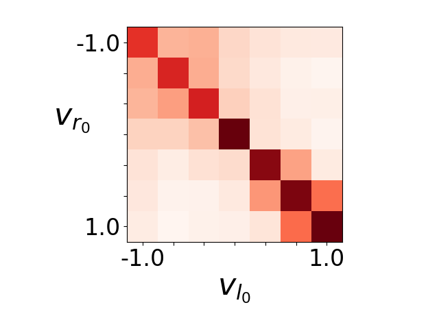
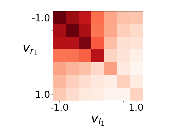
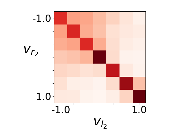
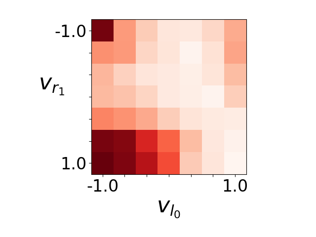
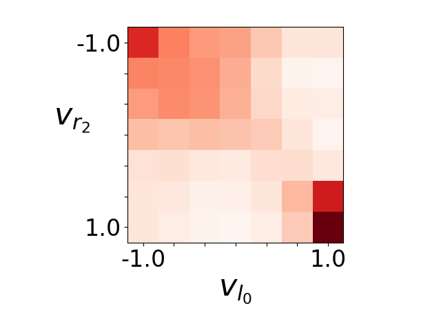
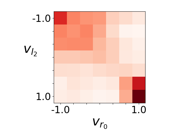
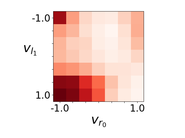
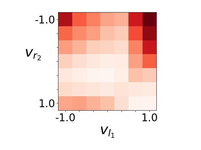
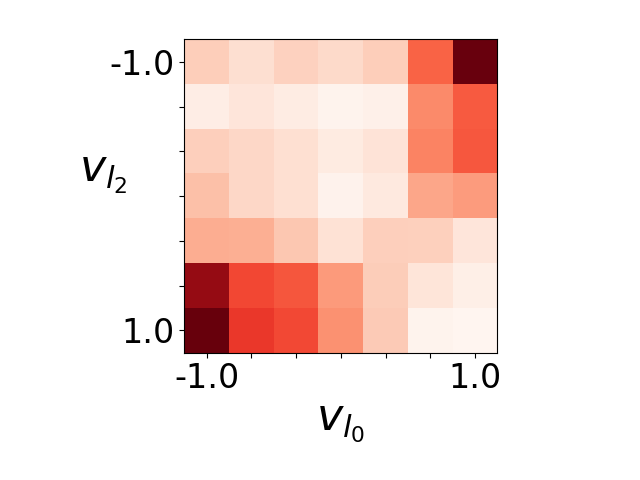
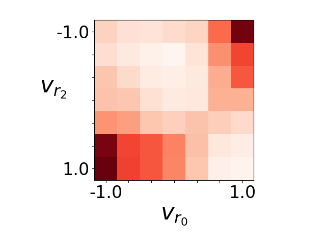
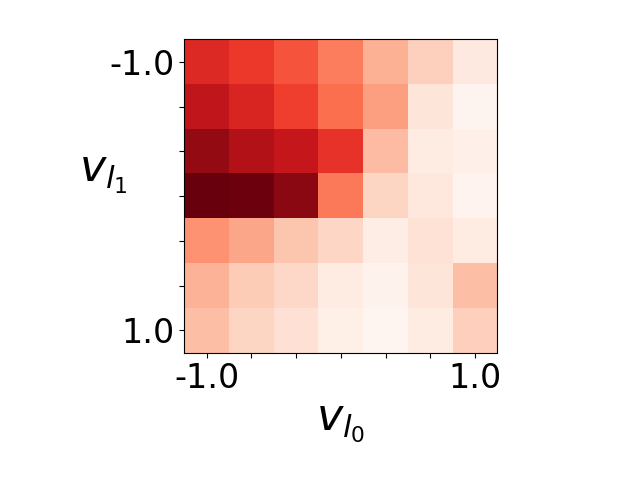
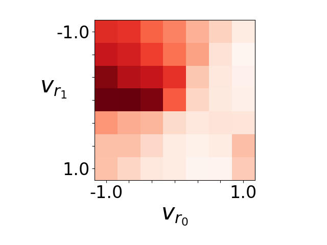
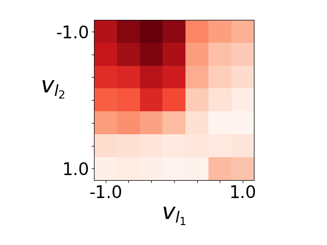
Figure 2: Heatmaps that relate relevant pairs of wheel speeds.

IV The Emergent Behavior

Visualizing grid search. The results of grid search are reported in Fig. 2. Because the search space is six-dimensional, we chose to visualize it by plotting every pair of parameters against each other. For example, we consider how the cost changes as $v_{\text{left}}^{S=0}$ and $v_{\text{right}}^{S=0}$ change. As an example of reading these plots, we can tell from the plot of $v_{\text{left}}^{S=1}$ and $v_{\text{right}}^{S=1}$ that there were no good controllers where the left and right wheel speeds were equal and negative (dark squares in the upper left), and that the best controllers had slightly unequal values close to 1 (lightest squares in the bottom left). These plots also convey the presence of sharp discontinuities where performance changes dramatically.

The emergent behavior. After running the grid search, the parameters with the lowest mean cost across all 38 configurations was

$$[1,-\nicefrac{{2}}{{3}},\nicefrac{{1}}{{3}},1,1,0].$$ (C)

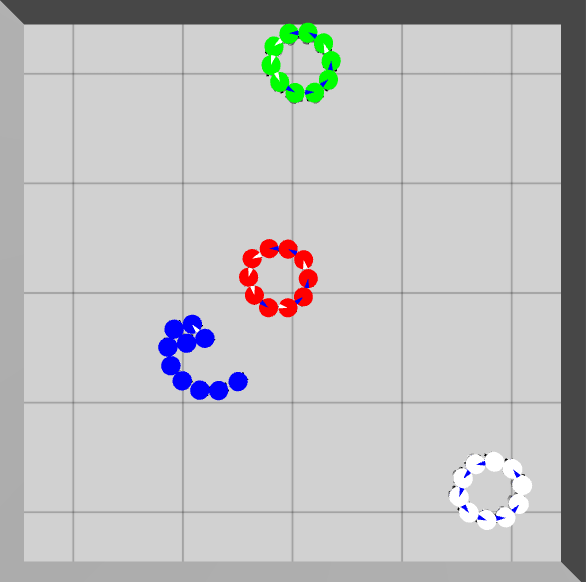
Figure 3: The segregation behavior found by grid search consists in the formation of homogeneous rings or spiraling structures that keep spinning over time. The rings tend to grow over time, disband, and reform.

The resulting behavior is for a robot to turn away from kin, but turn the opposite way when the robot sees nothing or non-kin. This behavior amounts to robots zig-zagging in a line towards their kin. As discussed in [10], when multiple robots execute this zig-zag behavior, spinning rings are formed. The remarkable aspect, in our case, is that spinning rings of kin robots emerge, eventually segregating the swarm in homogeneous groups. An example of this phenomenon as observed in simulated experiments is reported in Fig. 3. We also noted that occasionally the robots form spinning spiral shapes, which can also be seen in Fig. 3.

Interesting phenomena. It is important to note that, although we originally hoped that segregated clusters would be tightly packed, none of the top scoring parameters according to our cost function form tightly packed clusters. There are parameters which achieve tightly packed segregation, but they do so extremely slowly, and therefore our cost function correctly penalized them heavily for being too slow to be useful. In addition, we observed that the spinning rings formed by the robots tended to expand over time, disband into smaller structures, and eventually reappear. In addition, if a ring is disturbed by non-kin robots passing through it, the ring is disrupted but it eventually reforms. The growing and self-repairing dynamics is compatible with the findings in the work of St.-Onge et al. [10], in which ring formation is decomposed in four simpler behavioral traits: scouting, chaining, looping, and merging. This segregation behavior follows the same phases, and it constitutes a further example of structured space-time coordination arising from minimalistic assumptions on the capabilities of the robot. To better appreciate the dynamics of this behavior, we invite the interested reader to watch the videos at https://goo.gl/z8UAuB.

V Behavior Analysis

Using the parameter settings (C) as a basis, we now analyze the emerging behavior with the purpose of explaining how and why it emerges. In particular, we discuss the conditions under which segregation is guaranteed.

In the proofs, we employ the well-known equations that govern the instantaneous radius of curvature $R$ and rotation speed $\omega$ of the path followed a differential-drive robot with $l$ denoting the interwheel distance [19]:

$$R =\frac{l}{2}\frac{V_{\text{right}}+V_{\text{left}}}{V_{\text{right}}-V_{\text{left}}}=\frac{l}{2}\frac{v_{\text{right}}+v_{\text{left}}}{v_{\text{right}}-v_{\text{left}}}$$ (5)

$$\omega =\frac{V_{\text{right}}-V_{\text{left}}}{l}=\frac{V_{\text{max}}(v_{\text{right}}-v_{\text{left}})}{l}.$$

Theorem 1 (Scouting)

When a robot $i$ does not detect a kin, it turns clockwise until it finds one.

Proof:

The proof derives from the observation of the speeds in (C). When $S=0$ (no robot detected) and $S=2$ (non-kin detected), the left wheel speed is larger than the right one, producing a circular clockwise motion. Conversely, when $S=1$ (a kin is detected), the right wheel speed is larger than the left one, and the robot turns counterclockwise. ∎

Figure 4: A diagram for the geometry of motion towards kin robots. The red circle ($\mathbf{p}_{j}$) depicts the detected kin neighbor; the blue circle indicates the robot whose motion is being modeled ($\mathbf{p}_{i}$); the dashed green arc is the path followed by the robot, up to the limit point $\mathbf{q}_{i}$. Beyond the latter point, the blue robot ceases to move closer to the red robot.

Lemma 1 (Motion towards kin when kin detected)

A robot moves towards a kin robot if

$$V_{\text{max}}\Delta t\leq 3l\tan^{-1}\left[\frac{\sqrt{3}r}{l}\right].$$ (S1)

Proof:

When a robot encounters a kin, it picks the speeds $v_{\text{left}}^{S=1}=\nicefrac{{1}}{{3}}$ and $v_{\text{right}}^{S=1}=1$. This corresponds to a path that arcs counterclockwise, as reported in the diagram of Fig. 4. We indicate the position of the moving robot as $\mathbf{p}_{i}$ and the position of the kin as $\mathbf{p}_{j}$. For robot $i$ to move towards $j$, its trajectory path must be an arc that does not move past a limit point $\mathbf{q}_{i}$ because, beyond this point, the distance between $i$ and $j$ would increase. We can express this condition as

$$|\omega|\Delta t\leq\bar{\theta}$$

where $\bar{\theta}$ is the angle of the arc connecting $\mathbf{p}_{i}$ and $\mathbf{q}_{i}$.

Reasoning on the triangle formed by $\mathbf{p}_{i}$, $\mathbf{p}_{j}$ and the ICC, we can calculate

$$\bar{\theta}=2\tan^{-1}\frac{D}{|R|}$$ (6)

where we defined $D=\lVert\mathbf{p}_{i}-\mathbf{p}_{j}\rVert$. The right hand side of this inequality monotonically increases with $D$, hence to find the most strict condition we need to consider the smallest value of $D$ possible. This value corresponds to the situation in which $i$ and $j$ are tangent to each other; in this case, $D=\sqrt{3}r$, where $r$ indicates the robot radius (assumed identical for both robots). Using (5) with the values of $v_{\text{left}}^{S=1}$ and $v_{\text{right}}^{S=1}$, we obtain:

$$R =\frac{l}{2}\frac{1+\nicefrac{{1}}{{3}}}{1-\nicefrac{{1}}{{3}}}=l$$

$$\omega =\frac{V_{\text{max}}(1-\nicefrac{{1}}{{3}})}{l}=\frac{2}{3}\frac{V_{\text{max}}}{l}.$$

Plugging these expressions in (6), we obtain the statement. ∎

Lemma 2 (Motion towards kin when nothing detected)

Assume that a robot $i$ saw a kin $j$ at time $t-1$, has performed one step with $v_{\text{left}}^{S=1}$ and $v_{\text{right}}^{S=1}$, and at time $t$ it detects no robot. Robot $i$ moves towards the kin robot if

$$V_{\text{max}}\Delta t\leq\frac{6}{5}l\tan^{-1}\left[\frac{10\sqrt{3}r}{l}\right].$$ (S0)

Proof:

This proof follows the same reasoning as in Lemma 1 with the wheel speeds $v_{\text{left}}^{S=0}=1$ and $v_{\text{right}}^{S=0}=-\nicefrac{{2}}{{3}}$. ∎

Lemma 3 (Motion towards kin when non-kin detected)

Assume that a robot $i$ saw a kin $j$ at time $t-1$, has performed one step with $v_{\text{left}}^{S=1}$ and $v_{\text{right}}^{S=1}$, and at time $t$ it detects a non-kin. Robot $i$ moves towards the kin robot if

$$V_{\text{max}}\Delta t\leq 2l\tan^{-1}\left[\frac{2\sqrt{3}r}{l}\right].$$ (S2)

Proof:

This proof follows the same reasoning as in Lemma 1 with the wheel speeds $v_{\text{left}}^{S=2}=1$ and $v_{\text{right}}^{S=2}=0$. ∎

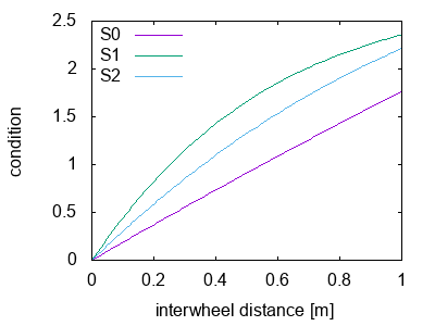
Figure 5: A graphical proof that (S0) is the strictest condition. The graph relates the length of the interwheel distance to the value of the conditions, for a constant value of the robot body radius.

.

Theorem 2 (Chaining)

A robot $i$ eventually follows a kin $j$ if (S0) holds.

Proof:

Because of Theorem 1, a robot that has not detected a kin rotates clockwise until it finds one. After this, the robot turns counterclockwise and, if (S1) holds, it steps closer to the kin. When the robot cannot detect the kin anymore it turns clockwise. If both (S0) and (S2) hold, then it is guaranteed robot $i$ moves closer to the kin. Eventually robot $i$ will see the kin again, and the cycle continues. This reasoning can be repeated for any pair of robots, and a chain self-sustains if the three conditions are satisfied at the same time. This occurs when the strictest among them holds. As shown graphically in Fig. 5, the strictest condition is (S0). ∎

Theorem 3 (Looping)

A chain of kin robots eventually forms a loop.

Proof:

When a chain is formed, the robot in front either detects a kin, in which case it follows it (thus growing the chain); or it does not detect a kin, in which case it moves clockwise until it detects one of the kin robots that follow it in the chain. Since every robot behind the front robot performs the chaining behavior, this results in the chain looping on itself until the tail is reached and the loop is closed. ∎

VI Experimental Results

VI-A Scalability Study

In this experiment we investigate how the segregation behavior scales with the number of classes and the number of robots in the environment. We varied the number of classes from 1 to 25 and ran 100 trials with robots uniformly randomly distributed.

Fixed number of robots per class. We studied the case in which every class has 10 robots. The results of this are plotted in Fig. 6. We observe that the cost increases with the number of classes. This occurs because, as the number of classes increases, the density of the robots increases too. Hence, line-of-sight occlusions between robots are more likely, navigation is more difficult, and the clusters do not have a chance to coalesce.

Fixed total number of robots. We considered the scenario in which a fixed number of robots is split into an increasing number of classes. We set the number of robots to 100, so with 25 classes 4 robots were still assigned to each class. As reported in Fig. 7, the cost is high for small numbers of classes but its value decreases fast and eventually oscillates lightly. The initial high cost is due to the fact that, with 100 robots to divided among few classes, it is difficult for every robot to join the same cluster. The clusters, instead, tend to form large islands of kins. As the number of classes increases, we conjecture that the oscillations are an artifact of the random initial conditions of each experiment.

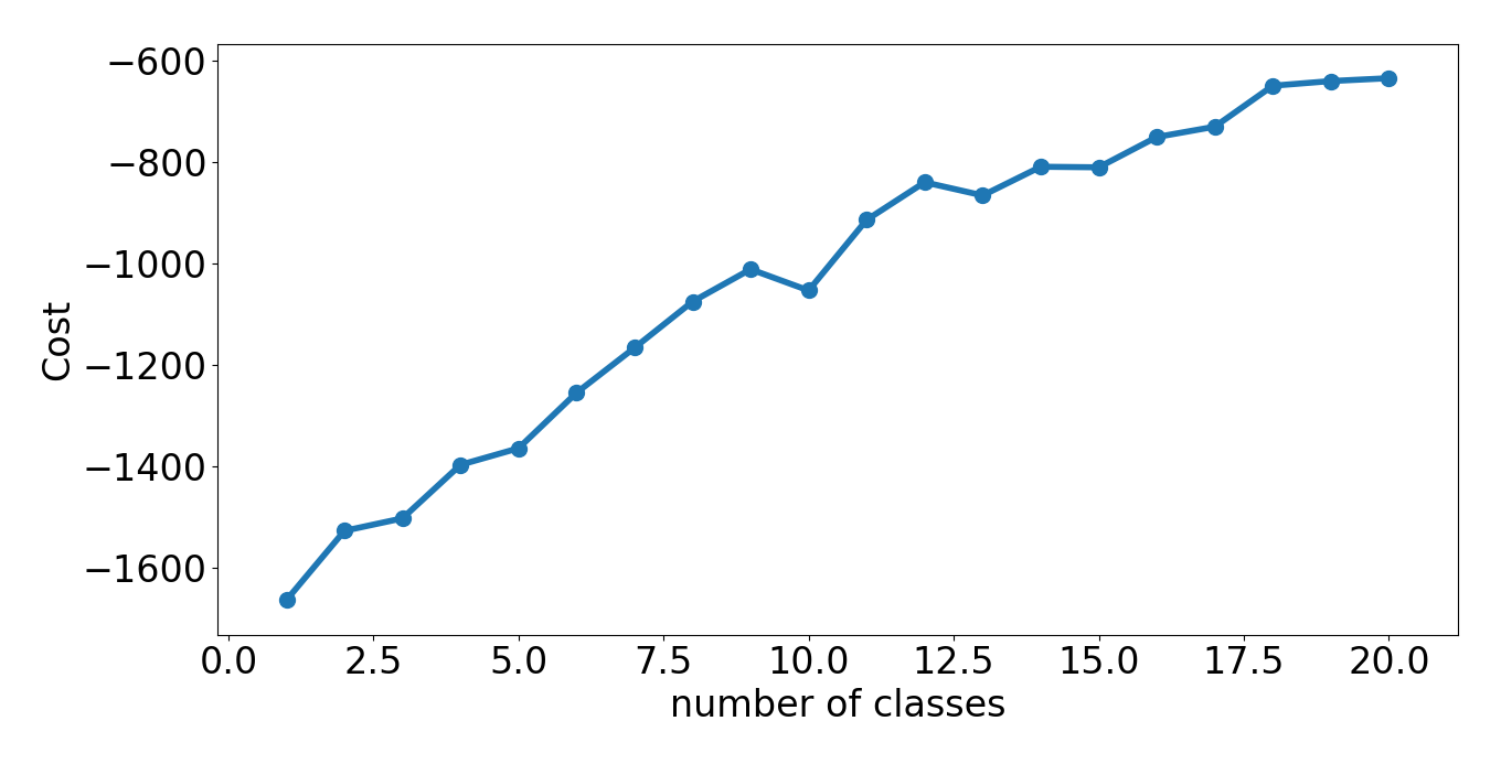
Figure 6: The average cost over 100 trials with $N$ classes, 10 robots per class.

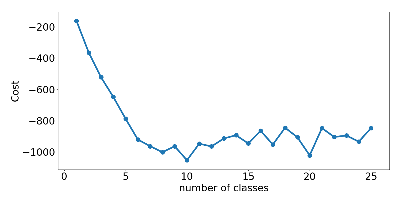
Figure 7: The average cost over 100 trials with 100 robots divided into $N$ classes.

VI-B The Effect of Implementation Details of the Sensor

We observed that the implementation details of the sensor have a significant effect on the behavior of the controller.

Initially, our method for determining sensor state from the simulated range-and-bearing system was to consider all the robots within some small angle in front of the robot and pick the closest one. This is very similar to what would be provided by a real-world camera that uses colored skirts on each robot and picks the largest blob as the robot to be detected. This sensor implementation works well and was used in the grid search experiments. However, we found later that, if the robots instead always prefer to react to kin over non-kin, larger rings form more quickly and robustly. For example, if there are two robots within the field of view of a robot’s sensor and the non-kin robot is closer, the robot would ignore it and execute the $S=1$ logic, which drives the robot towards the farther kin robot. Exploring exactly which of the various implementation details have what effect on cost is left for future work.

VI-C The Effect of the Beam Angle

On a real robot, there must be some finite beam angle to the theoretically line-of-sight sensor. We ran 100 trials in simulation with uniformly random initial distributions of 40 robots with various beam angles. Fig. 8 shows the results, along with a diagram showing how we define beam angle. The best beam angle we tested was $15\mathrm{°}$, and angles smaller or larger became progressively worse. We found that at lower beam angles, it was possible for a robot to become stuck in groups of two or three, and the robots spent all their time looking at each other instead of peeking around them to find kin. At larger angles, we suspect the behavior fails because larger beam angles cause the rings to enlarge faster, which in turn causes the rings to be so large that they are not considered a cluster anymore by our cost function.

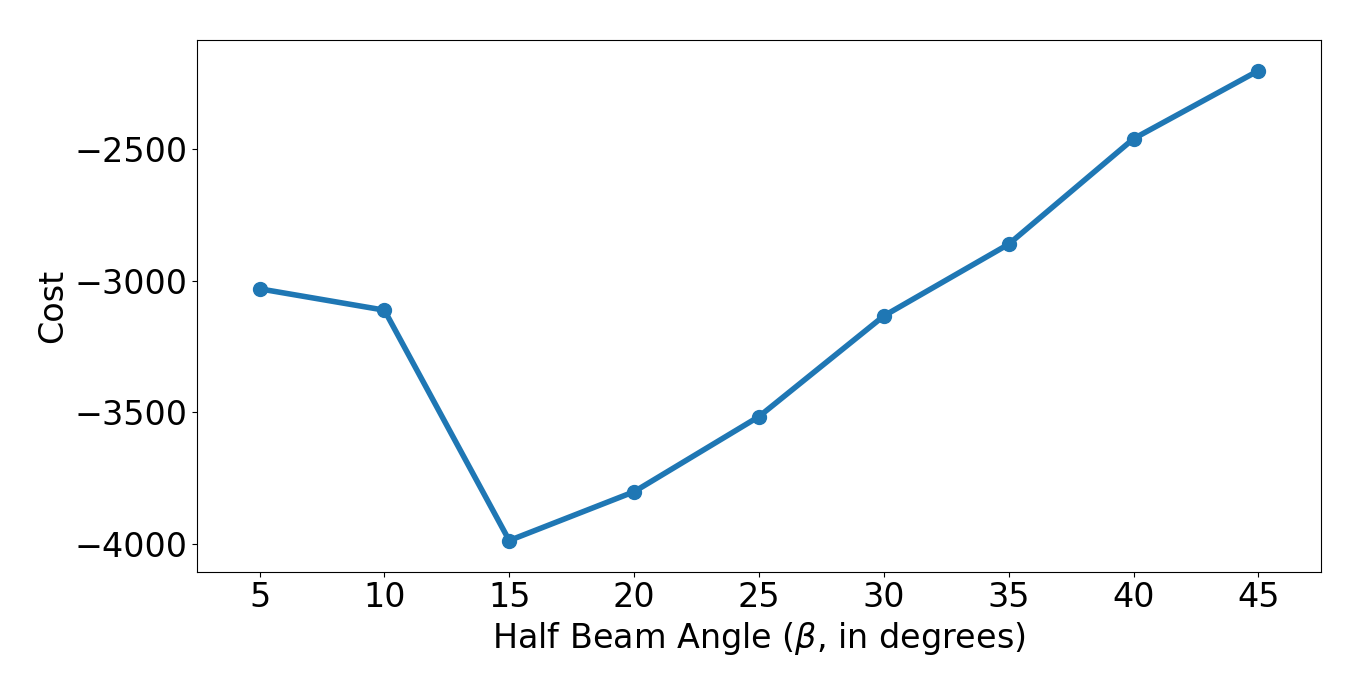
Figure 8: A $15\mathrm{°}$ degree half beam angle is best for segregation. Lower cost is better.

VI-D The Effect of Beam Length

We consider what happens if the theoretically infinite-range sensor has finite range. We use $15\mathrm{°}$ half beam angle and the same experimental setup as with the beam angle experiments. We consider the maximum range of the sensor as the diagonal length of the square in which the robot are initially distributed. In all our experiments, this square was $5\text{\,}\mathrm{m}$ on each side, so we consider a range of $7.07\text{\,}\mathrm{m}$ to be effectively unlimited. We report the costs for beam ranges as a fraction of this maximum range. As shown in Fig. 9, a beam range of 35% of the theoretical maximum performs just as well as an infinite sensor. Below this, the performance degrades. However, even a beam range of 7% of the maximum is more effective than zero range at segregation.

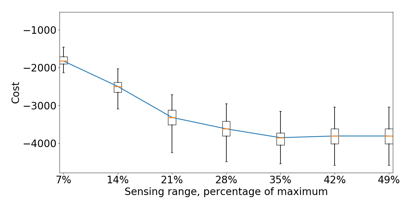
Figure 9: Segregation is robust to small sensor beam ranges. The performance at 35% of maximum range is indistinguishable from infinite range.

VII Conclusion

In this paper, we show how robots with only a ternary sensor and a controller which maps sensor readings to wheel speeds is capable of $N$-class segregation. This controller is invariant to the number of classes, and using the best found parameters we are able to construct formal guarantees on the emergent behavior. We performed a grid search to learn about the full parameter space, and we investigated the effect of sensor implementation details and the number of robots and classes on performance. Our findings indicate that robust segregation with non-ideal sensors in reality is possible, although not guaranteed.

References

- [1] M. Brambilla, E. Ferrante, M. Birattari, and M. Dorigo, “Swarm robotics: A review from the swarm engineering perspective,” Swarm Intelligence, vol. 7, no. 1, pp. 1–41, 2013.
- [2] M. Gauci, J. Chen, W. Li, T. J. Dodd, and R. Groß “Clustering Objects with Robots That Do Not Compute,” in Proceedings of the 2014 International Conference on Autonomous Agents and Multi-agent Systems, ser. AAMAS ’14. Richland, SC: International Foundation for Autonomous Agents and Multiagent Systems, 2014, pp. 421–428. [Online]. Available: http://dl.acm.org/citation.cfm?id=2615731.2615800
- [3] A. Bolger, M. Faulkner, D. Stein, L. White, and D. Rus, “Experiments in decentralized robot construction with tool delivery and assembly robots,” in 2010 IEEE/RSJ Int. Conf. on Intelligent Robots and Systems (IROS 2010). IEEE Press, 2010, pp. 5085–5092.
- [4] N. E. Shlyakhov, I. V. Vatamaniuk, and A. L. Ronzhin, “Survey of Methods and Algorithms of Robot Swarm Aggregation,” Journal of Physics: Conference Series, vol. 803, p. 012146, Jan. 2017. [Online]. Available: http://stacks.iop.org/1742-6596/803/i=1/a=012146?key=crossref.a3ceb0f2b8113f73c39aa6e56ddeeb8a
- [5] C. Pinciroli, A. Gasparri, E. Garone, and G. Beltrame, “Decentralized progressive shape formation with robot swarms,” in 13th International Symposium on Distributed Autonomous Robotic Systems (DARS2016), ser. Springer Proceedings in Advanced Robotics. Springer, November 2016, pp. 433–445.
- [6] R. Groß and M. Dorigo, “Self-assembly at the macroscopic scale,” Proceedings of the IEEE, vol. 96, no. 9, pp. 1490–1508, 2008.
- [7] M. Johnson and D. Brown, “Evolving and Controlling Perimeter, Rendezvous, and Foraging Behaviors in a Computation-Free Robot Swarm,” in Proceedings of the 9th EAI International Conference on Bio-inspired Information and Communications Technologies (Formerly BIONETICS), ser. BICT’15. ICST, Brussels, Belgium, Belgium: ICST (Institute for Computer Sciences, Social-Informatics and Telecommunications Engineering), 2016, pp. 311–314. [Online]. Available: http://dx.doi.org/10.4108/eai.3-12-2015.2262390
- [8] D. S. Brown, R. Turner, O. Hennigh, and S. Loscalzo, “Discovery and Exploration of Novel Swarm Behaviors Given Limited Robot Capabilities,” in Distributed Autonomous Robotic Systems, ser. Springer Proceedings in Advanced Robotics. Springer, Cham, 2018, pp. 447–460. [Online]. Available: https://link.springer.com.ezproxy.wpi.edu/chapter/10.1007/978-3-319-73008-0_31
- [9] M. Gauci, J. Chen, T. J. Dodd, and R. Groß “Evolving Aggregation Behaviors in Multi-Robot Systems with Binary Sensors,” in Distributed Autonomous Robotic Systems, ser. Springer Tracts in Advanced Robotics. Springer, Berlin, Heidelberg, 2014, pp. 355–367. [Online]. Available: https://link.springer.com/chapter/10.1007/978-3-642-55146-8_25
- [10] D. St-Onge, C. Pinciroli, and G. Beltrame, “Circle formation with computation-free robots shows emergent behavioral structure,” in Proceedings of the IEEE/RSJ International Conference on Intelligent Robots and Systems (IROS 2018). Madrid, Spain: IEEE Press, October 2018, in press.
- [11] E. Batlle and D. G. Wilkinson, “Molecular Mechanisms of Cell Segregation and Boundary Formation in Development and Tumorigenesis,” Cold Spring Harbor Perspectives in Biology, vol. 4, no. 1, p. a008227, Jan. 2012. [Online]. Available: http://cshperspectives.cshlp.org/content/4/1/a008227
- [12] M. S. Steinberg, “Reconstruction of tissues by dissociated cells,” Science, vol. 141, pp. 401–408, 1963.
- [13] N. N. Franks and A. Sendova-Franks, “Brood sorting by ants: distributing the workload over the work-surface,” Behavioral Ecology and Sociobiology, vol. 30, no. 2, pp. 109–123, 1992.
- [14] W. M. Spears, D. F. Spears, J. C. Hamann, and R. Heil, “Distributed, Physics-Based Control of Swarms of Vehicles,” Autonomous Robots, vol. 17, no. 2/3, pp. 137–162, Sep. 2004.
- [15] R. Groß S. Magnenat, and F. Mondada, “Segregation in swarms of mobile robots based on the Brazil nut effect,” in 2009 IEEE/RSJ International Conference on Intelligent Robots and Systems, Oct. 2009, pp. 4349–4356.
- [16] J. Chen, M. Gauci, M. J. Price, and G. R, “Segregation in swarms of e-puck robots based on the brazil nut effect,” in Proc. of the 11th Int. Conf. on Auton. Agents and Multi-agent Syst., 2012, pp. 163–170.
- [17] M. Kumar, D. P. Garg, and V. Kumar, “Segregation of Heterogeneous Units in a Swarm of Robotic Agents,” IEEE Transactions on Automatic Control, vol. 55, no. 3, pp. 743–748, Mar. 2010.
- [18] V. G. Santos, L. C. A. Pimenta, and L. Chaimowicz, “Segregation of multiple heterogeneous units in a robotic swarm,” in 2014 IEEE International Conference on Robotics and Automation (ICRA), May 2014, pp. 1112–1117.
- [19] G. Dudek and M. Jenkin, Computational Principles of Mobile Robotics, 2nd ed. Cambridge University Press, 2010.
- [20] C. Pinciroli, V. Trianni, R. O’Grady, G. Pini, A. Brutschy, M. Brambilla, N. Mathews, E. Ferrante, G. D. Caro, F. Ducatelle, M. Birattari, L. M. Gambardella, and M. Dorigo, “ARGoS: a Modular, Parallel, Multi-Engine Simulator for Multi-Robot Systems,” Swarm Intelligence, vol. 6, no. 4, pp. 271–295, 2012.
- [21] M. Bonani, V. Longchamp, S. Magnenat, P. Rétornaz, D. Burnier, G. Roulet, F. Vaussard, H. Bleuler, and F. Mondada, “The marXbot, a miniature mobile robot opening new perspectives for the collective-robotic research,” in Proceedings of the IEEE/RSJ International Conference on Intelligent Robots and Systems (IROS). Piscataway, NJ: IEEE Press, 2010, pp. 4187–4193.
- [22] M. Rubenstein, C. Ahler, and R. Nagpal, “Kilobot: A low cost scalable robot system for collective behaviors,” 2012 IEEE International Conference on Robotics and Automation, pp. 3293–3298, May 2012.