MgNet: A Unified Framework
of Multigrid and Convolutional Neural Network
Abstract
We develop a unified model, known as MgNet, that simultaneously recovers some convolutional neural networks (CNN) for image classification and multigrid (MG) methods for solving discretized partial differential equations (PDEs). This model is based on close connections that we have observed and uncovered between the CNN and MG methodologies. For example, pooling operation and feature extraction in CNN correspond directly to restriction operation and iterative smoothers in MG, respectively. As the solution space is often the dual of the data space in PDEs, the analogous concept of feature space and data space (which are dual to each other) is introduced in CNN. With such connections and new concept in the unified model, the function of various convolution operations and pooling used in CNN can be better understood. As a result, modified CNN models (with fewer weights and hyperparameters) are developed that exhibit competitive and sometimes better performance in comparison with existing CNN models when applied to both CIFAR-10 and CIFAR-100 data sets.
1 Introduction
This paper is devoted to the study of convolutional neural networks (CNN) lecun1998gradient; krizhevsky2012imagenet; goodfellow2017deep in machine learning by exploring their relationship with multigrid methods for numerically solving partial differential equation xu1992iterative; xu2002method; hackbusch2013multi. CNN has been successfully applied in many areas, especially computer vision lecun2015deep. Important examples of CNN include the LeNet-5 model of LeCun et al. in 1998 lecun1998gradient, the AlexNet of Hinton et el in 2012 krizhevsky2012imagenet, Residual Network (ResNet) of K. He et al. in 2015 he2016deep and other variants of CNN in simonyan2014very; szegedy2015going; huang2017densely. Given the great success of CNN models, it is of both theoretical and practical interest to understand why and how CNN works.
In 1990s, the mathematical analysis of DNN mainly focus on the approximation properties for DNN and CNN models. The first approximation results for DNN are obtained for a feedforward neural network with a single hidden layer separately in hornik1989multilayer and cybenko1989approximation. From 1989 to 1999, many results about the so-called expressive power of single hidden neural networks are derived barron1993universal; ellacott1994aspects; pinkus1999approximation. In recent, many new DNN structure with ReLU nair2010rectified activation function have been studied in connection with: wavelets shaham2018provable, finite element he2018relu, sparse grid montanelli2017deep and polynomial expansion e2018exponential. By using a connection of CNN and DNN that a convolution with large enough kernel can recover any linear mapping, zhou2018universality presents an approximate result with convergence rate by deep CNNs for functions in the Sobolev space with , see also most recent result of siegel2019approximation.
These function approximation theories for deep learning, are far from being adequate to explain why deep neural network, especially for CNN, works and to understand the efficiency of some successful models such as ResNet. One goal of this paper is to offer some mathematical insights into CNN by using ideas from multigrid methods and by developing a theoretical framework for these two methodologies from different fields. Furthermore, such insight is used to develop more efficient CNN models.
In the existing deep learning literature, ideas and techniques from multigrid methods have been used for the development of efficient deep neural networks. As a prominent example, the ResNet and iResNet developed in he2016deep; he2016identity, are motivated in part by the hierarchical use of “residuals” in multigrid methods as mentioned by the authors. As another example, in ronneberger2015u; milletari2016v, a CNN model with almost the same structure as the V-cycle multigrid is proposed to deal with volumetric medical image segmentation and biomedical image segmentation. More recently, multi-resolution images have been used as the input into the neural network in haber2017learning. ke2016multigrid use different net works to deal with multi-resolution images separately with a CNN to glue them together.
A dynamic system viewpoint has also been explored in many papers such as haber2017learning; e2017a; lu2018beyond to understand the iterative structure in ResNet type models such as the iResNet model in he2016identity:
| (1.1) |
Such an idea is further explored by li2017a to use some flow model to interpret the date flow in ResNet as the solution of transport equation following the characteristic line. chang2017multi proposes a multi-level training algorithm for the ResNet model by training a shallow model first and then prolongating its parameters to train a deeper model. lu2018beyond uses the idea of time discretization in dynamic systems to interpret PloyNet zhang2017polynet, FractalNet larsson2016fractalnet and RevNet gomez2017reversible as different time discretization schemes. Then they propose the LM-ResNet based on the idea of linear multi-step schemes in numerical ODEs with a stochastic learning strategy. long2018pde1; long2018pde2 construct the PDE-Net models to learn PDE model from data connecting discrete differential operators and convolutions.
In a different direction, new multigrid methods for numerical PDEs can be motivated by deep learning. For example, in katrutsa2017deep a Deep Multigrid Method is proposed where the restriction and prolongation matrices with a given sparsity pattern are trained by minimizing the Frobenius norm of a large power of the multigrid error propagation matrix with a sampling technique similar to what is used in machine learning. In hsieh2018learning, a linear U-net structure is proposed as a solver for linear PDEs on the regular mesh.
In this paper, we explore the connection between multigrid and convolutional neural networks, in several directions. First of all, we view the multi-scale of images used in CNN as piecewise (bi-)linear functions as used in multigrid methods, and we relate the pooling operation in CNN with the restriction operation in multigrid.
To examine further connections between CNN and multigrid, we introduce the so-called data and feature space for CNN, which is analogous to the function space and its duality in the theory of multigrid methods xu2017algebraic. With this new concept for CNN, we propose the data-feature mapping model in every grid as
| (1.2) |
where belongs to the data space and belongs to the feature space. The feature extraction process can then be obtained through an iterative procedure for solving the above system, namely
| (1.3) |
with . The above iterative scheme (1.3) can be interpreted as both the feature extraction step in ResNet type models and the smoothing step in multigrid method.
Using the above observations and new concepts, we develop a unified framework, called MgNet, that simultaneously recovers some convolutional neural networks and multigrid methods. Furthermore, we establish connections between several ResNet type models using the MgNet framework. We provide improvements/generalizations of several ResNet type models that are as competitive as and sometimes more efficient than existing models, as demonstrated by numerically experiments for both CIFAR-10 and CIFAR-100 krizhevsky2009learning.
The remaining sections are organized as follows. In § 2, we introduce some notation and preliminary results in supervised learning especially for image classification problem. In § 3, we present the idea that we need to distinguish the data and feature space in CNN models and introduce some related mappings. In § 4, we explore the structures and operators when we consider images as (bi-)linear functions in multilevel grids. In § 5, we introduce multigrid by splitting it into two phases. In § LABEL:sec:mgnet, we give an abstract form of MgNet as a framework for multigrid and convolutional neural network with details. In § LABEL:sec:CNNs, we introduce some classical CNN structures with rigorous mathematical definition. In § LABEL:sec:relation, we construct some relations and connections between MgNet and classic models. In § LABEL:sec:numerics, we present some numerical results to show the efficiency of MgNet. In § LABEL:sec:conclusion we give concluding remarks.
2 Supervised learning on image classification
We consider a basic machine learning problem for classifying a collection of images into distinctive classes. As an example, we consider a two-dimensional image which is usually represented by a tensor
Here
| (2.1) |
A typical supervised machine learning problem begins with a data set (training data)
with
and is the label for data , with as the probability for in classes .
Roughly speaking, a supervised learning problem can be thought as data fitting problem in a high dimensional space . Namely, we need to find a mapping
such that, for a given ,
| (2.2) |
if is in class , for . For the general setting above, we use a probatilistic model for understanding the output as a discrete distribution on , with as the probability for in the class , namely
| (2.3) |
At last, we finish our model with a simple strategy to choose
| (2.4) |
as the label for a test data , which ideally is close to (2.2). The remaining key issue is the construction of the classification mapping .
The main step in the construction of is to construct a nonlinear mapping
| (2.5) |
with
| (2.6) |
To be consistent with the notation for CNN which will be described below, here the subscript refers to the number of coarsening girds in CNN. Roughly speaking, the map plays two roles. The first role is to conduct a dimensionality reduction, namely
The second role is to map a complicated set of data into a set of data that are linearly separable. As a result, the simple logistic regression procedure can be applied.
The first step in a logistic regression is to introduce a linear mapping:
as
| (2.7) |
where , .
We then use the soft-max function.
| (2.8) |
to obtain a logistic regression model
| (2.9) |
By combining the nonlinear mapping in (2.5) and the logistic regression (2.9), we obtain the following classifier:
| (2.10) |
Given the model (2.10), we finish the training phase with solving the next optimization problem:
| (2.11) |
where Here is a loss function that measures the predicted result and the real label . In logistic regression, the following cross-entropy loss function is often used
3 Data space, feature space and relevant mappings
Given a data
| (3.1) |
where is called the spatial dimension and is the channel dimension.
For the given data in (3.1), we look for some feature vector, denoted by , associated with :
| (3.2) |
We make an assumption that the data and feature are related by a mapping (which can be either linear or nonlinear)
| (3.3) |
so that
| (3.4) |
A mapping
is called a feature extractor if and
| (3.5) |
is such that .
The data-feature relationship (3.4) or (3.5) is not unique. Different relationships give rise to different features. We can view the data-feature relationship given in (3.4) as a model that we propose. Here the mapping , which can be either linear or nonlinear, is unknown and needs to be trained.
We point out that the data space and feature space may have different numbers of channels.
3.1 A special linear mapping: convolution
One important class of linear mapping is the so-called convolution:
that can be defined by
| (3.6) |
where is a matrix with all elements being , and for
| (3.7) |
The coefficients in (3.7) constitute a kernel matrix
| (3.8) |
where is often taken as small integers. Here padding means how to choose when is out of or . Those next three choices are often used
| (3.9) |
if
| (3.10) |
Here means the remainder when is divided by .
The operation (3.12) is also called a convolution with stride 1. More generally, given an integer , a convolution with stride for is defined as:
| (3.13) |
Here denotes the smallest integer that greater than . In CNN, we often take .
3.2 Some linear and nonlinear mappings and extractors
A data-feature map and feacture extractor can be either linear or nonlinear. The nonlinearity can be obtained from appropriate application of an activation function
| (3.14) |
In this paper, we mainly consider a special activation function, known as the rectified linear unit (ReLU), which is defined by
| (3.15) |
By applying the function to each component, we can extend this
| (3.16) |
A linear data-feature mapping can simply given by a convolution as in (3.7):
| (3.17) |
A nonlinear mapping can be given by compositions of convolution and activation functions:
| (3.18) |
and
| (3.19) |
Here , and are all appropriate convolution mappings.
3.3 Iterative feature extraction schemes
One key idea in this paper is that we consider different iterative processes to approximately solve (3.4) and relate them to many existing popular CNN models. Here, let us assume that the feature-data mapping (3.4) is given as a linear form (3.17). We next propose some iterative schemes to solve (3.4) for an appropriately chosen .
-
•
Residual correction method,
(3.20) Here can be chosen as linear like or nonlinear like (3.19). The reason why is taken the nonlinear form as in (3.19) will be discussed later based on our main discovery about the relationship between MgNet and iResNet as discussed in § LABEL:sec:CNNs and § LABEL:sec:relation. We refer to xu1992iterative for more discussion on iterative schemes in the form of (3.20).
-
•
Semi-iterative method for accelerating the residual correction iterative scheme,
(3.21) where and . Letting the residual for , the following iterative scheme for is implied by (3.21)
(3.22) because of the linearity of . This scheme is analogous to the DenseNet huang2017densely which will be discussed more in § LABEL:sec:CNNs and below. More discussion on semi-iterative method for linear system can be found in hackbusch1994iterative; golub2012matrix.
-
•
Chebyshev semi-iterative method,
(3.23) The above scheme can be obtained from the above semi-iterative form by applying the Chebyshev polynomial theory hackbusch1994iterative; golub2012matrix. Similar to the previous case, considering the iterative form of the residual , (3.23) implies that
(3.24) This scheme corresponds to the LM-ResNet in lu2018beyond which was obtained as a linear multi-step scheme for some underlying ODEs.
4 Piecewise (bi-)linear functions on multilevel grids
An image can be viewed as a function on a grid. Images with different resolutions can then be viewed as functions on grids of different sizes. The use of such multiple-grids is a main technique used in the standard multigrid method for solving discretized partial differential equations xu1992iterative; xu2002method, and it can also be interpreted as a main ingredient used in convolutional neural networks (CNN).
Without loss of generality, for simplicity, we assume that the initial grid, , is of size
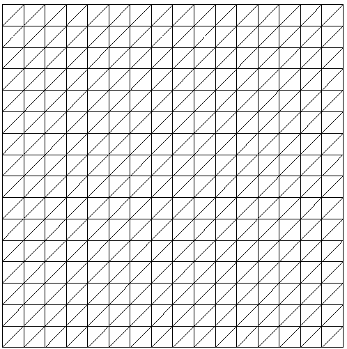
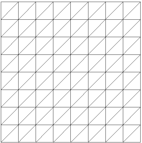
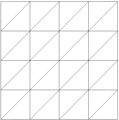
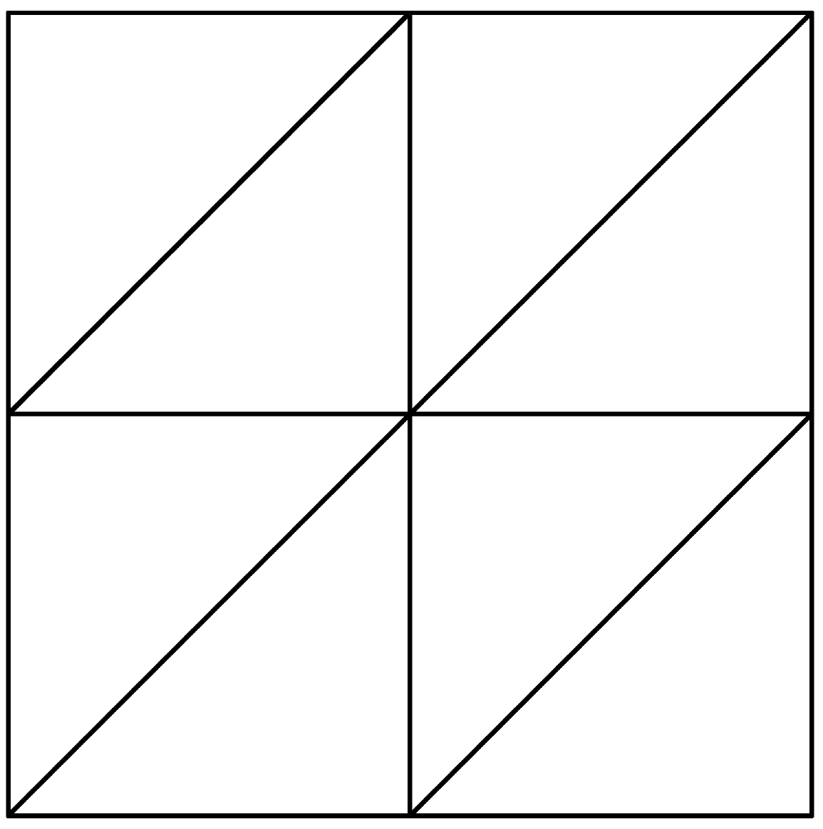
for some integers . Starting from , we consider a sequence of coarse grids (as depicted in Fig. 1 with ):
| (4.1) |
such that consist of grid points, with
| (4.2) |
The grid points of these grids can be given by
Here and , for some . The above geometric coordinates are usually not used in image precess literatures, but they are relevant in the context of multigrid method for numerical solution of PDEs. We now consider piecewise linear functions on the sequence of grids (4.1) and we obtain a nested sequence of linear vector spaces
| (4.3) |
Here each consists of all piecewise bilinear (or linear) functions with respect to the grid (4.1) and (4.2). Each has a set of basis functions: satisfying:
Thus, for each , we have
| (4.4) |
4.1 Prolongation
Given a piecewise (bi-)linear function , the nodal values of on grids point constitute a tensor
We note that thanks to (4.3) and the nodal values of on constitute a tensor
Using the property of piecewise (bi-)linear functions, it is easy to see that
| (4.5) |
where
| (4.6) |
which is called a prolongation in multigrid terminology. More specifically,
| (4.7) |
with
| (4.8) |
and
| (4.9) |
4.2 Pooling, restriction and interpolation
The prolongation given by (4.6) can be used to transfer feature from a coarse grid to a fine grid. On the other hand, we also need a mapping, known as restriction, that transfer data from fine grid to corse grid:
| (4.10) |
In multigrid for solving discretized partial differential equation, the restriction is often taken to be transpose of the prolongation given by (4.6):
| (4.11) |
Lemma 1.
If takes the form of prolongation in multigrid methods for linear finite element functions on the above grids, then is a convolution with stride and a kernel as:
| (4.12) |
where, if is piecewise bilinears,
| (4.13) |
or, if is piecewise linears,
| (4.14) |
In addition, all these convolutions are applied with zero padding as in (3.9) , which is consistent with the Neumann boundary condition for applying FEM to numerical PDEs. More details will be discussed in § 4.2.
In the deep learning literature, the restriction such as (4.10) is often known as pooling operation. One popular pooling is a convolution with stride , with some small integer .
Some other fixed (or untrained) poolings are also often used. One popular pooling is the so-called average pooling which can be a convolution with stride or bigger using the kernel in the form of
| (4.15) |
Nonlinear pooling operator is also used, for the example the max-pooling operator with stride as follows:
| (4.16) |
Another approach to the construction of restriction of pooling can be obtained by using interpolation. Given
let be the function whose nodal values are precisely give by as in (4.4). Any reasonable linear operator
| (4.17) |
such as: nodal value interpolation, Scott-Zhang interpolation and projection xu2019FEM, would give rise to a mapping
| (4.18) |
such that
As situations permit, we can use these a priori given restrictions to replace unknown pooling operators to reduce the number of parameters.
5 Multigrid methods for numerical PDEs
Let us first briefly describe a geometric multigrid method used to solve the following boundary value problem
| (5.1) |
We consider a continuous linear finite element discretization of (5.1) on a nested sequence of grids of sizes with , as shown in the left part of Fig. 1 and the corresponding sequence of finite element spaces (4.3).
Based on the grid , the discretized system is
| (5.2) |
Here, is a tensor satisfying
| (5.3) |
which holds for with zero padding. Here we notice that, there exists a kernel as
| (5.4) |
with
| (5.5) |
Where is the stander convolution operation with zero padding like (3.7). We now briefly describe a simple multigrid method by a mixed use of the terminologies from deep learning goodfellow2017deep and multigrid methods.
The first main ingredient in GMG is a smoother. A commonly used smoother is a damped Jacobi with damped coefficient with , which can be written as satisfying
| (5.6) |
for equation (5.2) with initial guess zero. If we apply the Jacobian iteration twice, then
with element-wise form
| (5.7) |
Then we have
| (5.8) |
and
| (5.9) |
such that
| (5.10) |
Similarly, we can define .
We use prolongation as defined in (4.6) and restriction . Further more, we use the following relationship to define coarse operation
| (5.11) |
with .
Using the smoother , prolongation , restriction and mapping as given in (5.11), we can formulate the following algorithm as a major component of a multigrid algorithm.
Algorithm 1