Studying gaugino masses in supersymmetric model at future 100 TeV $pp$ collider

Abstract

We discuss prospects of studying supersymmetric model at future $pp$ circular collider (FCC) with its centre-of-mass energy of $\sim 100\ {\rm TeV}$. We pay particular attention to the model in which Wino is lighter than other supersymmetric particles and all the gauginos are within the kinematical reach of the FCC, which is the case in a large class of so-called pure gravity mediation model based on anomaly mediated supersymmetry breaking. In such a class of model, charged Wino becomes long-lived with its decay length of $\sim 6\ {\rm cm}$, and the charged Wino tracks may be identified in particular by the inner pixel detector; the charged Wino tracks can be used not only for the discrimination of standard model backgrounds but also for the event reconstructions. We show that precise determinations of the Bino, Wino, and gluino masses are possible at the FCC. For such measurements, information about the charged Wino tracks, including the one about the velocity of the charged Wino using the time of the hit at the pixel detector, is crucial. With the measurements of the gaugino masses in the pure gravity mediation model, we have an access to more fundamental parameters like the gravitino mass.

1 Introduction

There are strong motivations to consider physics beyond the standard model (BSM) at TeV scale. One is dark matter that cannot be explained in the framework of the standard model; particularly, the scenario of thermal relic dark matter requires the annihilation cross section of the dark matter particle to be $\sim 1\ {\rm pb}$, which is the typical cross section for particles with the mass scale $\sim 0.1$–$1\ {\rm TeV}$. In addition, a large hierarchy between the electroweak scale and the Planck scale, i.e. the scale of the gravity, motivates us to consider some mechanism to relax the quadratic divergence in the Higgs mass parameter in the standard model.

High-energy-collider experiments are crucial for the study of BSM physics. LHC experiments have been searching for the BSM particles as an energy-frontier, but no direct sign has been discovered yet. Although LHC experiments will keep on exploring BSM particles at higher mass scale, BSM particles may be just above the discovery reach of the LHC. In this case, a collider with higher energy than the LHC is needed to discover and study the BSM physics. Among possibilities, we consider $pp$ option of Future Circular Collider (FCC) with the centre-of-mass energy of $\sim 100\ {\rm TeV}$ Mangano:2016jyj ; Contino:2016spe ; Golling:2016gvc because it can drastically push up the energy frontier of high-energy experiments. Because the FCC is considered to be one of promising collider experiments, the understanding of the physics potential of the FCC is of high importance.

Here, we discuss the prospect of the FCC in the study of supersymmetric (SUSY) model. We concentrate on the so-called pure gravity mediation (PGM) model of SUSY breaking Ibe:2006de ; Ibe:2011aa ; ArkaniHamed:2012gw , which is strongly motivated from theoretical and phenomenological points of view. As we will discuss in the next section, in the PGM model, scalar particles in the minimal SUSY standard model (MSSM) have masses of $O(100)\ {\rm TeV}$ and may be too heavy to be studied at the FCC. However, gaugino masses are generated by the anomaly mediation Randall:1998uk ; Giudice:1998xp and are loop suppressed relative to the scalar masses. Typically, the gauginos are at the TeV scale and are within the reach of the FCC. Such a spectrum is easily obtained by a simple set up of the SUSY breaking sector. In addition, the PGM model has several advantages in cosmology. In particular, a thermally produced lightest superparticle (LSP) can be a viable candidate of dark matter under the assumption of $R$-parity conservation ArkaniHamed:2006mb .

One important feature of the model of our interest, the PGM model, is that the Winos, which are the gauginos for $SU(2)_{L}$ gauge group, are likely to be lighter than other superparticles. In particular, due to the radiative correction, the neutral Wino $\tilde{W}^{0}$ is slightly lighter than charged ones $\tilde{W}^{\pm}$ Cheng:1998hc ; Feng:1999fu and hence is the LSP. With such a mass spectrum, charged Wino has a relatively long lifetime and, once produced at the FCC, it may fly a macroscopic distance of $\sim 10\ {\rm cm}$ before its decay. The track of such a “long-lived” charged Wino may be identified by the inner pixel detector of the FCC, which provides a very characteristic and unique signal of the PGM model. The characteristic signal is used in searches for the Wino in LHC experiments and exclusion limits of Wino masses are set by the ATLAS ATLAS:2018 and CMS CMS:2018 experiments. The discovery reaches of this type of searches at the FCC have been studied in, for example, ref. Low:2014cba ; Cirelli:2014dsa . The charged Wino tracks expected in the PGM model can be used not only for the discovery but also for the study of the properties of SUSY particles.

In this paper, we discuss the prospect of the study of SUSY particles at the FCC, paying particular attention to the PGM model of SUSY breaking. We mainly focus on a parameter region where all the gauginos, i.e, Bino, Winos, and gluino, are within the reach of the FCC, assuming that its centre-of-mass energy is $100\ {\rm TeV}$. We propose procedures to measure Wino, Bino, and gluino masses at the FCC, using the pair production process of gluinos, $pp\rightarrow\tilde{g}\tilde{g}$, and the pair production process of charged Winos associated with hard jets, $pp\rightarrow\tilde{W}^{+}\tilde{W}^{-}+\mathrm{jets}$. We show that information about the charged Wino tracks from the inner pixel detector is crucial not only for the background reduction but also for the reconstruction of SUSY events. We also point out that, for the gaugino mass determination, it is important to precisely determine the velocity of charged Wino, which is expected to be possible by using the time information available from the pixel detector.

The organization of this paper is as follows. In section 2, we introduce the PGM model and introduce several Sample Points for our Monte Carlo (MC) analysis. In section 3, we explain basic features of the SUSY events at the FCC. The results of the MC analysis for the gaugino mass determinations are shown in section 4. Implications of the gaugino mass determinations for the understanding of the underlying theory are discussed in section 5. Section 6 is devoted to conclusions and discussions.

2 Model

Let us first introduce the SUSY model we consider. Among various possibilities, we concentrate on the so-called pure gravity mediation (PGM) model of SUSY breaking Ibe:2006de ; Ibe:2011aa ; ArkaniHamed:2012gw based on anomaly mediation Randall:1998uk ; Giudice:1998xp . In this model, the sfermion and Higgsino masses are generated by (tree-level) Planck-suppressed operators and are of the order of the gravitino mass $m_{3/2}$. On the contrary, assuming that there is no singlet field in the SUSY breaking hidden sector so that tree-level gaugino masses in the MSSM sector are forbidden, the gaugino masses are obtained from the effect of anomaly mediation. In this model, the gaugino masses are one-loop suppressed compared to the gravitino mass. Then, the gauginos are relatively light and are the primary targets of collider experiments.

In the PGM model, the SUSY breaking gaugino mass parameters for $U(1)_{Y}$, $SU(2)_{L}$, and $SU(3)_{C}$ gauge interactions, denoted as $M_{1}$, $M_{2}$, and $M_{3}$, respectively, are given as Giudice:1998xp ; Gherghetta:1999sw

$$M_{1}(M_{\rm S})= \,\frac{g_{1}^{2}(M_{\rm S})}{16\pi^{2}}\left(11m_{3/2}+L\right),$$ (1)

$$M_{2}(M_{\rm S})= \,\frac{g_{2}^{2}(M_{\rm S})}{16\pi^{2}}\left(m_{3/2}+L\right),$$ (2)

$$M_{3}(M_{\rm S})= \,\frac{g_{3}^{2}(M_{\rm S})}{16\pi^{2}}\left(-3m_{3/2}\right),$$ (3)

where $g_{1}$, $g_{2}$, and $g_{3}$ are gauge-coupling constants of $U(1)_{Y}$, $SU(2)_{L}$, and $SU(3)_{C}$ gauge interactions, respectively. Here, $L$ denotes the effect of the threshold correction due to the Higgs and Higgsino loop and is given by

$$L\equiv\mu\sin 2\beta\frac{m_{A}^{2}}{|\mu|^{2}-m_{A}^{2}}\ln\frac{|\mu|^{2}}{m_{A}^{2}},$$ (4)

where $\mu$ and $m_{A}$ are the SUSY invariant Higgs mass and the pseudo-scalar Higgs mass, respectively, while $\beta$ being the angle parametrizing the relative sizes of vacuum expectation values of up- and down-type Higgses. In addition, $M_{\rm S}$ is the mass scale of sfermions and Higgsinos, and hence $M_{\rm S}\sim m_{3/2}$. Here and hereafter, we take the convention such that $m_{3/2}$ is real and positive. We use the $\overline{\mathrm{MS}}$ scheme for the calculation of gauge coupling constants and mass parameters.

In general, $M_{1}$, $M_{2}$, and $M_{3}$ are complex and depend on the renormalization scale. The gaugino masses (i.e. mass eigenvalues) are determined from $M_{1}$, $M_{2}$, and $M_{3}$ at the renormalization scale close to the mass eigenvalues. The mass eigenvalues of Bino, Wino, and gluino, which are real and positive, are denoted as $m_{\tilde{B}}$, $m_{\tilde{W}}$, and $m_{\tilde{g}}$, respectively. We take into account the one-loop threshold correction to the gluino mass Giudice:2004tc

$$m_{\tilde{g}}=|M_{3}(M_{\mathrm{G}})|\left[1+\frac{g_{3}^{2}}{16\pi^{2}}\left(12+9\ln\frac{M_{\mathrm{G}}^{2}}{|M_{3}|^{2}}\right)\right],$$ (5)

where $M_{\mathrm{G}}$ is the mass scale of gauginos, which we determine by solving $M_{\mathrm{G}}=|M_{3}(M_{\mathrm{G}})|$ in our analysis. In addition, we neglect the small threshold corrections to Bino and Wino at the gaugino mass scale and just take $m_{\tilde{B}}=|M_{1}(M_{\mathrm{G}})|$ and $m_{\tilde{W}}=|M_{2}(M_{\mathrm{G}})|$. When $m_{3/2}$ and $L$ are of the same order of magnitude, Wino becomes lighter than Bino and gluino.

In our analysis, we consider the case where the gravitino mass is of $O(100)\ {\rm TeV}$ (and hence the sfermion and Higgsino masses are), while the gaugino masses are of $O(1)\ {\rm TeV}$. Such a mass spectrum is phenomenologically viable and well-motivated:

• The observed value of the Higgs mass (i.e. $m_{h}\simeq 125\ {\rm GeV}$ Tanabashi:2018oca ) can be realized due to radiative corrections Okada:1990vk ; Okada:1990gg ; Ellis:1990nz ; Ellis:1991zd ; Haber:1990aw .

• Neutral Wino is a viable candidate of dark matter. In particular, if $m_{\tilde{W}}\simeq 2.9\ {\rm TeV}$, thermal relic density of Wino becomes equal to the present dark matter density Hisano:2006nn . In addition, even if the Wino mass is smaller than $\sim 2.9\ {\rm TeV}$, Wino dark matter is possible with non-thermal production Giudice:1998xp ; Moroi:1999zb .

• With the large gravitino mass of $O(100)\ {\rm TeV}$, a dangerous cosmological gravitino problem can be avoided even if the reheating temperature after inflation is as high as $O(10^{9})\ {\rm GeV}$ Kawasaki:2017bqm . A simple scenario of leptogenesis Fukugita:1986hr works with such reheating temperature Buchmuller:2004nz ; Giudice:2003jh .

• Even if the sfermion and Higgsino masses are as high as $O(100)\ {\rm TeV}$, the gauge coupling constants still meet at $\sim 10^{16}\ {\rm GeV}$, and the SUSY grand unified theory, which is one of the strong motivations to consider SUSY models, is still viable Giudice:2004tc .

• Because of large sfermion masses, CP and flavour violations due to the loops of SUSY particles are suppressed. This will significantly relax the SUSY CP and flavour problems Moroi:2013sfa ; McKeen:2013dma .

Although there exist motivations to adopt the mass spectrum mentioned above, we note here that the model of our interest requires a sizeable tuning of parameters to realize viable electroweak symmetry breaking. This is due to the hierarchy between the mass scale of superparticles and the electroweak scale. We also comment, however, that the hierarchy here is significantly reduced compared to that between the Planck and the electroweak scales which causes the naturalness problem in the standard model (assuming that the cut-off scale is the Planck scale).

Because the neutralino dark matter is one of the strong motivations of low-energy SUSY, we consider the case that the Wino becomes lighter than the Bino and gluino so that neutral Wino becomes the candidate of dark matter. (Notice that, in the present framework, the Bino hardly becomes a viable candidate of dark matter even if it is the LSP. This is because, with heavy sfermions and Higgsinos, its pair annihilation cross section is too small to realize the correct relic density to be dark matter.) In particular, we assume that the Wino mass is $\sim 2.9\ {\rm TeV}$ so that the thermal relic density of Wino becomes consistent with the present dark matter density.

In the following, we adopt several Sample Points for our MC analysis. The mass spectrum and fundamental parameters are summarized in table 1. As shown in table 1, $m_{\tilde{W}}<m_{\tilde{B}}<m_{\tilde{g}}$ in all Sample Points.

Assuming $R$-parity conservation, gluino decays as

$$\tilde{g}\rightarrow\bar{q}q\tilde{B},~{}~{}~{}\bar{q}q^{(\prime)}\tilde{W},$$

where $q$ and $\bar{q}$ denote the standard-model quark and anti-quark, respectively. The branching ratio for each decay mode depends on the mass spectrum of squarks. If the masses of left- and right-handed squarks are the same, the branching ratio for the latter process becomes larger than the former. However, if the mass of the right-handed squarks are lighter than the left-handed ones, they can be comparable (or $\mathrm{Br}\,(\tilde{g}\rightarrow\bar{q}q\tilde{B})$ may even become larger than $\mathrm{Br}\,(\tilde{g}\rightarrow\bar{q}q^{(\prime)}\tilde{W})$). The mass spectrum of the squarks is strongly model-dependent; it depends on dimension-6 operators connecting (s)quark chiral multiplets and SUSY breaking fields in the Kähler potential. Because the detail of the squark mass spectrum is currently unknown, we simply assume that

$$\mathrm{Br}\,(\tilde{g}\rightarrow\bar{q}q\tilde{B})=\mathrm{Br}\,(\tilde{g}\rightarrow\bar{q}q^{(\prime)}\tilde{W})=0.5,$$ (6)

and that the decay process is flavour universal. Such branching ratios are realized when the masses of right-handed squarks are smaller than those of left-handed ones by a factor of a few. We note here that one of the motivations of the assumptions mentioned above are to demonstrate the possibility of the Bino mass determination as we explain in the following. The dominant decay modes of Bino are given by

$$\tilde{B}\rightarrow\tilde{W}^{\pm}W^{\mp},~{}~{}~{}\tilde{W}^{0}h,$$

and, when $|\mu|\gg|M_{1,2}|\gg m_{W,h}$ (with $m_{W}$ and $m_{h}$ being the $W$-boson mass and Higgs mass, respectively), the decay rates are approximately given by

$$\Gamma_{\tilde{B}\to\tilde{W}^{\pm}W^{\mp}} =\frac{\beta_{\tilde{W}^{\pm}W^{\mp}}\kappa^{2}}{8\pi}m_{\tilde{B}}\left(1+\frac{m_{\tilde{W}}}{m_{\tilde{B}}}\right)^{2}\left[1+\frac{2m_{W}^{2}}{(m_{\tilde{B}}+m_{\tilde{W}})^{2}}\right]\left[1-\frac{m_{W}^{2}}{(m_{\tilde{B}}-m_{\tilde{W}})^{2}}\right],$$ (7)

$$\Gamma_{\tilde{B}\to\tilde{W}^{0}h} =\frac{\beta_{\tilde{W}^{0}h}\kappa^{2}}{8\pi}m_{\tilde{B}}\left[\left(1+\frac{m_{\tilde{W}}}{m_{\tilde{B}}}\right)^{2}-\frac{m_{h}^{2}}{m_{\tilde{B}}^{2}}\right],$$ (8)

where

$$\beta_{\tilde{W}^{\pm}W^{\mp}}^{2}=\frac{m_{\tilde{B}}^{4}-2(m_{\tilde{W}^{\pm}}^{2}+m_{W}^{2})m_{\tilde{B}}^{2}+(m_{\tilde{W}^{\pm}}^{2}-m_{W}^{2})^{2}}{m_{\tilde{B}}^{4}},$$ (9)

and $\beta_{\tilde{W}^{0}h}^{2}$ is obtained by replacing $m_{\tilde{W}^{\pm}}\to m_{\tilde{W}^{0}}$ and $m_{W}\to m_{h}$ in the above formula. In addition, $\kappa\equiv g_{1}g_{2}v\sin\beta\cos\beta\mu^{-1}$ with $v\simeq 174\,\mathrm{GeV}$ being the vacuum expectation value of the Higgs boson. The masses of charged and neutral Winos split after the electroweak symmetry breaking. When $|\mu|$ is much larger than the electroweak scale, which is the case in the present framework, the mass splitting is dominantly via radiative correction due to loop diagrams with electroweak gauge bosons Cheng:1998hc ; Feng:1999fu , and the neutral Wino becomes lighter than the charged one. Based on the two-loop calculation, the mass splitting is $\delta m_{\tilde{W}}\simeq 165\ {\rm MeV}$ Ibe:2012sx ; then charged Wino dominantly decays as $\tilde{W}^{\pm}\rightarrow\tilde{W}^{0}\pi^{\pm}$ with

$$c\tau_{\tilde{W}^{\pm}}\simeq 5.75\ {\rm cm},$$ (10)

where $\tau_{\tilde{W}^{\pm}}$ is the proper lifetime of charged Wino while $c$ is the speed of light.

	Point 1	Point 2	Point 3
$m_{3/2}$ [TeV]	$250$	$302$	$350$
$L$ [TeV]	$800$	$756$	$709$
$m_{\tilde{B}}$ [GeV]	$3660$	$4060$	$4470$
$m_{\tilde{W}}$ [GeV]	$2900$	$2900$	$2900$
$m_{\tilde{g}}$ [GeV]	$6000$	$7000$	$8000$
$\sigma(pp\rightarrow\tilde{g}\tilde{g})$ [fb]	$7.9$	$2.7$	$1.0$

Table 1: Fundamental parameters ($m_{3/2}$ and $L$), gaugino masses, and the gluino pair production cross section (for the centre-of-mass of $100\ {\rm TeV}$), for Sample Points 1, 2, and 3.

3 SUSY events at the FCC

In this section, we discuss important features of SUSY events at the FCC which are used for our analysis. In the sample points of our choice, gluino is within the kinematical reach of the FCC, and its pair production process is the primary target. Hereafter, we consider the pair production process of gluinos, $pp\rightarrow\tilde{g}\tilde{g}$, and the pair production process of charged Winos associated with a high-$p_{T}$ jet, $pp\rightarrow\tilde{W}^{+}\tilde{W}^{-}+\mathrm{jets}$. From these processes we extract information about the gaugino masses as we discuss in the following.

3.1 Background estimation

In order to eliminate standard-model backgrounds, we use the fact that charged Wino tracks, which are disappearing and high-$p_{T}$, may be recognized by the inner pixel detector. In the gluino pair production events, each gluino decays down to a charged or neutral Wino. Although charged Wino is unstable, it has a sizeable lifetime and its $c\tau_{\tilde{W}^{\pm}}$ is about $5.75\ {\rm cm}$ that is of the same order of the distance to the pixel detector from the interaction point. Thus, once a charged Wino is produced, it may hit several layers of the pixel detector before its decay into a neutral Wino and a pion. Charged Wino track is expected to be (i) short (i.e. disappearing in the tracker), and (ii) high-$p_{T}$; such a track is hardly realized by a single standard-model particle. Another source of fake Wino-like track is due to an accidental alignment of hits of particles mainly from pile-ups and it is the dominant source according to ref. Saito2019 . In addition, in the signal events (i.e. the gluino pair production events), the missing transverse momentum evaluated only from jets is likely to be large because of the momenta carried away by Winos; this is not expected in the background events that have fake Wino-like tracks.

The gaugino mass reconstruction in our analysis is based on the events satisfying the following requirements:

• Requirement 1: There is a “long enough” Wino-like track. The transverse length of the track, denoted as $L_{T,1}$, should be longer than $L_{T,1}^{\rm(min)}=10\ {\rm cm}$. In addition, the pseudo-rapidity ($\eta$) of the track is required to be $|\eta|<1.5$.

• Requirement 2: There is another “long enough” Wino-like track. The transverse length of the track, denoted as $L_{T,2}$ should be longer than $L_{T,2}^{\rm(min)}$. As we will discuss later, $L_{T,2}^{\rm(min)}$ is set to be $10\ {\rm cm}$ but results with $L_{T,2}^{\rm(min)}=5\ {\rm cm}$ are also shown to see how the event selection affects on the mass determination. In addition, the pseudo-rapidity of the track is required to be $|\eta|<1.5$.

• Requirement 3: The missing transverse momentum should be larger than $1\ {\rm TeV}$.

We use signal events in which the decay chain of each gluino contains a charged Wino. We assume that the charged Wino with a longer (shorter) transverse flight length in an event can be fully identified when the transverse flight length is longer than $L_{T,1}^{\rm(min)}$ ($L_{T,2}^{\rm(min)}$).

According to ref. Saito2019 , the probability to have one fake disappearing track in the pseudorapidity range of $|\eta|<1.5$ is about $2\times 10^{-5}$ per bunch crossing, requiring hits in five pixel layers for a particular setup of the FCC experiment. The background rate can be reduced therefore by ten orders of magnitude by requiring both Requirement 1 and Requirement 2. Additionally, the Requirement 3 can also reduce them as well. As a result, standard-model backgrounds can be negligible by applying these requirements.

3.2 Wino velocity measurement

We assume that the information about the velocity of the charged Wino will be available if the flight length is long enough. It may be possible that each pixel layer determines the time of the hit with the resolution of $O(10)\ {\rm ps}$ by utilizing, for example, low-gain avalanche detectors Pellegrini2014 ; Lange2017 , with which the velocity relative to the speed of light ($\beta$) of the charged Wino could be determined with the accuracy of $O(1)\ \%$. We estimate the expected accuracy of the $\beta$ measurement via a simple MC analysis. We generate straight tracks, and smear the time of hits at each pixel-detector layers to determine the “observed” times of hits. The time of the $pp$ collision (which can be identified as the time when Winos are produced) is assumed to be accurately determined by using associated jets. Then, the observed $\beta$ is determined for each track by fitting the observed times of hits by a linear function assuming a constant $\beta$. The accuracy is estimated as the standard deviation of the distribution of the difference between the observed and the generator-level velocities as a function of the generator-level $\beta$. Then the average accuracy for Wino tracks is estimated by taking the weighted average using the generator-level $\beta$ distribution in our Wino samples. We found that, assuming the hit-level time resolution of $20\ {\rm ps}$ ($40\ {\rm ps}$), the Wino velocity can be determined with the accuracy of $3.0\ \%$ and $3.3\ \%$ ($6.1\ \%$ and $6.8\ \%$) for charged Winos reaching the pixel layer located at the transverse length of $10\ {\rm cm}$ with $\beta<0.8$ and $0.9$, respectively. We require that the transverse flight length should be longer than $10\ {\rm cm}$ for the $\beta$ measurement, and assume that the resolution of the observed Wino $\beta$ is $6\ \%$.

3.3 MC simulation

The flowchart of our MC analysis is shown in figure 1. We use MadGraph5_aMC@NLO (v2.6.3.2) Alwall:2011uj ; Alwall:2014hca to generate $pp\rightarrow\tilde{g}\tilde{g}$ and $pp\rightarrow\tilde{W}^{+}\tilde{W}^{-}+\mathrm{jets}$ events. Then, decay and hadronization processes are taken care of by PYTHIA8 Sjostrand:2014zea . A fast detector simulation is performed by Delphes (v3.4.1) deFavereau:2013fsa ; we use the card FCChh.tcl included in the package. Because the velocity measurement of charged Wino cannot be simulated by the Delphes package by default, the information about Winos provided by PYTHIA8, as well as Delphes outputs, are passed to our original analysis code; the analysis code smears the velocities of charged Winos to determine observed velocities, applies kinematical cuts, reconstructs kinematical variables (including invariant masses that will be discussed in the following), and performs the hemisphere analysis. In particular, for charged Winos whose transverse flight length $L_{T}$ is longer than $10\ {\rm cm}$, the observed value of the Wino velocity is determined by

$$\beta=(1+6\ \%\times Z)\beta^{\rm(true)},$$ (1)

where $\beta$ and $\beta^{\rm(true)}$ are observed and true values of the velocity, and $Z$ is the $(0,1)$ Gaussian random variable. An accurate velocity determination may be difficult for charged Winos with a short transverse flight length, for example, $L_{T}<10\ {\rm cm}$; thus Winos with $L_{T}<10\ {\rm cm}$ are not used in the mass determination. The fittings of invariant-mass distributions are performed by ROOT (v6.14) Brun:1997pa .

Figure 1: The flowchart of our MC analysis.

4 Gaugino mass determination

Now we are at the position of discussing how and how well we can determine the gaugino masses. In order to demonstrate that the gaugino mass determinations are possible, we generate $pp\rightarrow\tilde{g}\tilde{g}$ and $pp\rightarrow\tilde{W}^{+}\tilde{W}^{-}+\mathrm{jets}$ events. Then, we study the reconstructions of gaugino masses using data sets which correspond to multiple experiments with a fixed integrated luminosity ${\cal L}$ for each experiment. As for $pp\rightarrow\tilde{g}\tilde{g}$ process, we take ${\cal L}=10\ {\rm ab}^{-1}$ for Sample Points 1 and 2, while ${\cal L}=30\ {\rm ab}^{-1}$ for Sample Point 3. For $pp\rightarrow\tilde{W}^{+}\tilde{W}^{-}+\mathrm{jets}$ process, we take ${\cal L}=30\ {\rm ab}^{-1}$.

4.1 Wino mass determination

We first consider the measurement of the Wino mass. Using charged Winos identified as short high-$p_{T}$ tracks with velocity information, we may determine Wino mass if the momentum of the Winos are known. Even though the curvature of the track depends on the Wino momentum, most of the Winos are so high-$p_{T}$ that precise determination of the curvature is expected to be unlikely.

Instead of using the curvature information, we use the conservation of the transverse momentum to determine the Wino momenta. Because we use events with two charged Wino tracks, the directions of the Wino momenta (which we denote $\vec{n}_{\tilde{W}_{1}^{\pm}}$ and $\vec{n}_{\tilde{W}_{2}^{\pm}}$) are known. Then, the momenta of charged Winos, $\vec{P}_{\tilde{W}_{I}^{\pm}}$ with $I=1$ and $2$, are given in the following form:

$$\vec{P}_{\tilde{W}_{I}^{\pm}}=c_{I}\vec{n}_{\tilde{W}_{I}^{\pm}},$$ (1)

with $c_{I}$ being constants. The constants $c_{1}$ and $c_{2}$ can be obtained by using the transverse momentum conservation. Concentrating on events in which the decay products of gluinos contain only hadrons and Winos, the following relation should be held:

$$\left[\sum_{I=1}^{2}\vec{P}_{\tilde{W}_{I}^{\pm}}+\sum_{j:{\rm jets}}\vec{p}_{j}\right]_{T}=0,$$ (2)

where the subscript $T$ denotes transverse components. In our analysis, we use Eq. (2) to calculate $c_{1}$ and $c_{2}$, with which Wino momenta are determined. With $\vec{P}_{\tilde{W}_{I}^{\pm}}$ being given, the reconstructed Wino mass (in association with each track) is given by

$$m_{\tilde{W}}^{\rm(rec)}=\frac{\sqrt{1-\beta_{I}^{2}}}{\beta_{I}}|\vec{P}_{\tilde{W}_{I}}|,$$ (3)

where $\beta_{I}$ is the measured velocity of the $I$-th charged Wino.

In order to see how well the Wino mass can be reconstructed, we study the distribution of $m_{\tilde{W}}^{\rm(rec)}$. For the Wino mass determination utilizing the above procedure, charged Wino samples with smaller uncertainties in the boost factor are necessary; this motivates us to use charged Winos with relatively low velocity. In addition, because the “missing” momentum evaluated using the jet momenta is assumed to be compensated by the Wino momenta, events with neutrino emission should be excluded in this study. Thus, we do not use events with an isolated lepton because it may originate from the decay of $W$-boson. Thus, for the Wino mass determination, we use the events satisfying the following conditions (as well as Requirements 1, 2 and 3 in the previous section):

• There exists a charged Wino with $L_{T}>10\ {\rm cm}$ and $\beta<0.8$.

• There exists no isolated lepton.

We calculate the reconstructed Wino mass $m_{\tilde{W}}^{\rm(rec)}$ for all the charged Winos satisfying (1a).

Figure 2: Distribution of the reconstructed Wino mass for Sample Point 1, taking $L_{T,2}^{\rm(min)}=10\ {\rm cm}$ (left) and $5\ {\rm cm}$ (right) in a single experiment with the integrated luminosity of ${\cal L}=10\ {\rm ab}^{-1}$.

Figure 3: Distribution of the reconstructed Wino mass for Sample Point 2, taking $L_{T,2}^{\rm(min)}=10\ {\rm cm}$ (left) and $5\ {\rm cm}$ (right) in a single experiment with the integrated luminosity of ${\cal L}=10\ {\rm ab}^{-1}$.

Figure 4: Distribution of the reconstructed Wino mass for Sample Point 3, taking $L_{T,2}^{\rm(min)}=10\ {\rm cm}$ (left) and $5\ {\rm cm}$ (right) in a single experiment with the integrated luminosity of ${\cal L}=30\ {\rm ab}^{-1}$.

In figures 2, 3, and 4, we show the distribution of the reconstructed Wino mass for Sample Points 1, 2, and 3, respectively, where not only $L_{T,2}^{\rm(min)}=10\ {\rm cm}$ but also $5\ {\rm cm}$ cases are shown as explained before. As mentioned earlier, the Wino with $L_{T,2}^{\rm(min)}=5\ {\rm cm}$ is not used for the mass determination; it is used to show impact on the mass determination from altering the event selections. This is also the case for Bino and gluino. For Sample Points 1 and 2 (Sample Point 3), we take the integrated luminosity ${\cal L}$ of $10\ {\rm ab}^{-1}$ ($30\ {\rm ab}^{-1}$). The peak of the distribution is close to the true Wino mass. In order to determine the position of the peak, we use a fitting function in the form of a Gaussian function plus a constant:

$$\frac{dN}{dm^{\rm(rec)}}=A\exp\left[-\frac{(m^{\rm(rec)}-\bar{m})^{2}}{2\sigma^{2}}\right]+C,$$ (4)

where $\bar{m}$, $\sigma$, $A$, and $C$ are fitting parameters. In each figure, the fitting function with the best-fit parameters is shown in the red line. The best-fit value of $\bar{m}$, denoted as Mwno(Gauss), is also shown in each figure.

We expect to extract information about the Wino mass from the position of the Gaussian peak (i.e. the peak of the fitting function). The position of the peak may not exactly agree with the true Wino mass even with large enough statistics. We expect that this is due to our choice of the fitting function given in eq. (4), and that we may find a better fitting function without such a systematic effect. The detailed study of the fitting function is beyond the scope of this paper, and we simply assume that the relation between characteristic features of the fitting function (like the position of the peak) and the true mass can be well understood by, for example, a reliable MC analysis. In addition, as indicated in the figures, the statistical uncertainty in the measurement of the Wino mass is accounted for. Here, we evaluate the statistical uncertainty by using 100 independent data sets for each Sample Point; we determine the position of the Gaussian peak for each data set, and the standard deviation of the peak position is regarded as the statistical uncertainty in the Wino mass determination. The statistical uncertainty as well as the mean of the peak position based on 100 data sets are summarized in table 2.

	$L_{T,2}^{\rm(min)}=10\ {\rm cm}$			$L_{T,2}^{\rm(min)}=5\ {\rm cm}$
	Point 1	Point 2	Point 3	Point 1	Point 2	Point 3
$\langle m_{\tilde{W}}\rangle_{100}$	2922	2915	2896	2907	2891	2891
$\delta m_{\tilde{W}}$	75	109	92	44	71	57

Table 2: The mean of the peak position based on 100 data sets of $pp\rightarrow\tilde{g}\tilde{g}$ events for each Sample Point, denoted as $\langle m_{\tilde{W}}\rangle_{100}$, as well as the uncertainty in the Wino mass determination (in units of GeV).

So far, we have only considered the $pp\rightarrow\tilde{g}\tilde{g}$ process to determine the Wino mass. However, if gluino is so heavy that the cross section for the gluino pair production is significantly suppressed, it may be more efficient to use the electroweak production of charged Winos. In particular, the process $pp\rightarrow\tilde{W}^{+}\tilde{W}^{-}+\mathrm{jets}$ may be used for the Wino mass determination, where a large missing transverse momentum is necessary to determine the Wino momenta as well as to pass the trigger selection. Here, we study such a possibility assuming that $m_{\tilde{W}}=2.9\,\mathrm{TeV}$ and that the gluino is out of kinematical reach of the FCC. With this choice of the Wino mass, we performed the MC simulation of the processes up to two hard jets and obtained $\sigma(pp\rightarrow\tilde{W}^{+}\tilde{W}^{-}+\mathrm{jets})\simeq 0.15\,\mathrm{fb}$ for the missing transverse momentum larger than $1\,\mathrm{TeV}$. As for the event selection, we require the same requirements as the previous analysis, i.e. Requirements 1, 2, and 3 in the previous section and conditions (1a) and (1b) in this section. We assume that standard-model backgrounds do not exist after requiring two (long enough) charged Wino tracks. Then, we determine the reconstructed Wino mass using eq. (3) for each Wino track.

Figure 5: Distribution of the reconstructed Wino mass for the chargino pair production process, taking $L_{T,2}^{\rm(min)}=10\ {\rm cm}$ (left) and $5\ {\rm cm}$ (right) in a single experiment with the integrated luminosity of ${\cal L}=30\ {\rm ab}^{-1}$.

	$L_{T,2}^{\rm(min)}=10\ {\rm cm}$	$L_{T,2}^{\rm(min)}=5\ {\rm cm}$
$\langle m_{\tilde{W}}\rangle_{100}$	2751	2754
$\delta m_{\tilde{W}}$	128	84

Table 3: The mean of the peak position based on 100 data sets $pp\rightarrow\tilde{W}^{+}\tilde{W}^{-}+\mathrm{jets}$ events, denoted as $\langle m_{\tilde{W}}\rangle_{100}$, as well as the uncertainty in the Wino mass determination (in units of GeV).

In figure 5, we show the distribution of the reconstructed Wino mass, taking the integrated luminosity $\mathcal{L}$ of $30\,\mathrm{ab}^{-1}$. We can see that, with $\mathcal{L}\sim 30\,\mathrm{ab}^{-1}$, we may observe a peak close to the true Wino mass. We also perform a fit using the fitting function given in eq. (4). From the figure, one can see the statistical uncertainty in the fit and the difference between the true Wino mass and the position of the Gaussian peak. Although the difference is larger than in the case of $pp\rightarrow\tilde{g}\tilde{g}$ events, we again assume that the dependence of the position of the peak on the true mass can be well understood by a reliable MC analysis and so on. Under this assumption, we evaluate the statistical uncertainty with 100 independent event sets as we described before and summarize the result in table 3.

4.2 Bino mass determination

Next, we consider the Bino mass determination. Here, we use the decay mode $\tilde{B}\rightarrow\tilde{W}^{\pm}W^{\mp}$, which has a sizeable branching ratio in the present case. Assuming that the Wino mass is known (see the previous subsection), the Wino four-momentum can be determined by using the velocity information (or by the conservation of the transverse momentum). Thus, we may reconstruct the Bino mass by calculating the invariant mass of the $\tilde{W}^{\pm}$ plus $W$-boson system, if the decay products of the $W$-boson are identified.

For this purpose, we use the fact that the $W$-boson produced by the Bino decay may be highly boosted. The hadronic decay products of the boosted $W$-boson may result in a single fat jet with the jet mass $m_{j}$ close to the $W$-boson mass. In figure 6, we show the distribution of the jet mass for Sample Point 1. We can observe a peak at $m_{j}\sim m_{W}$. Thus, if we require $m_{j}\sim m_{W}$, we can obtain $W$-rich samples of jets. Using such a jet, with denoting its four-momentum as $p_{j}$, the reconstructed Bino mass is defined as

$$m_{\tilde{B}}^{\rm(rec)}=\sqrt{(m_{\tilde{W}}^{\rm(rec)}u_{\tilde{W}}+p_{j})^{2}},$$ (5)

where $u_{\tilde{W}}$ is the four-velocity of the charged Wino:

$$u_{\tilde{W}}=\frac{1}{\sqrt{1-\beta^{2}}}(1,\beta\vec{n}_{\tilde{W}}),$$ (6)

with $\vec{n}_{\tilde{W}}$ being the direction of the Wino momentum determined by the track information.

Figure 6: The jet-mass distribution for the Sample Point 1.

Among the events with two charged Wino tracks (i.e. events that meet Requirements 1, 2, and 3 in the previous section), those satisfying the followings are used for the Bino mass reconstruction:

• There exists a charged Wino with $L_{T}>10\ {\rm cm}$ and $\beta<0.9$. (In order to increase the number of samples, we adopt a larger value of the maximal velocity compared to the Wino mass determination.)

• There exists a fat jet with $70\ {\rm GeV}<m_{j}<90\ {\rm GeV}$, with $m_{j}$ being the jet mass. We call such a jet as “$W$-jet.”

We calculate the reconstructed Bino mass given in eq. (5) for all the pairs of a charged Wino satisfying (2a) and a $W$-jet satisfying (2b).

Figure 7: Distribution of $m_{\tilde{B}}^{\rm(rec)}$ for Sample Point 1, taking $L_{T,2}^{\rm(min)}=10\ {\rm cm}$ (left) and $5\ {\rm cm}$ (right) in a single experiment with the integrated luminosity of ${\cal L}=10\ {\rm ab}^{-1}$.

Figure 8: Distribution of $m_{\tilde{B}}^{\rm(rec)}$ for Sample Point 2, taking $L_{T,2}^{\rm(min)}=10\ {\rm cm}$ (left) and $5\ {\rm cm}$ (right) in a single experiment with the integrated luminosity of ${\cal L}=10\ {\rm ab}^{-1}$.

Figure 9: Distribution of $m_{\tilde{B}}^{\rm(rec)}$ for Sample Point 3, taking $L_{T,2}^{\rm(min)}=10\ {\rm cm}$ (left) and $5\ {\rm cm}$ (right) in a single experiment with the integrated luminosity of ${\cal L}=30\ {\rm ab}^{-1}$.

In figures 7$\,\mathchar 45\relax\mathchar 45\relax\,$9, we show the distribution of the reconstructed Bino mass for Sample Points $1\,\mathchar 45\relax\mathchar 45\relax\,3$, respectively. Here, the true value of the Wino mass is used for the calculation of the four-momenta of charged Winos. We can see that, in each figure, the peak of the histogram is close to the true Bino mass and hence the Bino mass determination is possible via the method using the charged Wino track and the $W$-jet. We use the fitting function given in eq. (4) to estimate the position of the peak. The fitting function with the best-fit parameters is shown in the red line. For each Sample Point, the best-fit value of the position of the Gaussian peak (denoted as Mbno(Gauss)) and its statistical uncertainty are shown in the figure.

There exist several sources of uncertainties in the reconstructed Bino mass. We observe a slight deviation of the position of the Gaussian peak from the true Bino mass. We found that the position of the peak of the fitting function is likely to be lower than the true Bino mass with the present choice of cut parameters. Such a systematic effect in the fitting is assumed to be corrected by, for example, a reliable MC analysis, and hence is not included in the estimation of the uncertainty in the Bino mass measurement. The position of the Gaussian peak should also have a statistical uncertainty. As in the case of the Wino mass determination, the statistical uncertainty (denoted as $\delta m_{\tilde{B}}^{\rm(stat)}$) is determined by using 100 independent data sets for each Sample Point. Furthermore, so far, we have used the true Wino mass as an input for the analysis. As we discussed in the previous subsection, the Wino mass is also a parameter that should be experimentally determined, and the uncertainty in the measured Wino mass becomes a source of the uncertainty in the reconstructed Bino mass. In order to see how large such an effect is, we estimate the change of the reconstructed Bino mass with respect to the change of the input Wino mass. With varying the input Wino mass by $100\ {\rm GeV}$, we found that the reconstructed Bino mass changes by $\sim 100\ {\rm GeV}$. Thus, we take $\delta m_{\tilde{B}}^{(m_{\tilde{W}})}\sim\delta m_{\tilde{W}}$, where $\delta m_{\tilde{B}}^{(m_{\tilde{W}})}$ is the uncertainty associated with Wino mass uncertainty $\delta m_{\tilde{W}}$ in the reconstructed Bino mass. We add all the uncertainties in quadrature to estimate the expected accuracy of the Bino mass measurement. The uncertainties in the Bino mass reconstruction, as well as the mean of the peak position based on 100 data sets, are summarized in table 4.

	$L_{T,2}^{\rm(min)}=10\ {\rm cm}$			$L_{T,2}^{\rm(min)}=5\ {\rm cm}$
	Point 1	Point 2	Point 3	Point 1	Point 2	Point 3
$\langle m_{\tilde{B}}\rangle_{100}$	3651	4036	4394	3651	4036	4397
$\delta m_{\tilde{B}}^{\rm(stat)}$	15	36	42	10	25	29
$\delta m_{\tilde{B}}^{(m_{\tilde{W}})}$	75	109	92	44	71	57
$\delta m_{\tilde{B}}$	76	115	101	45	75	64

Table 4: The mean of the peak position based on 100 data sets for each Sample Point, denoted as $\langle m_{\tilde{B}}\rangle_{100}$, as well as the uncertainty in the Bino mass determination (in units of GeV). The total uncertainty, $\delta m_{\tilde{B}}$, is obtained by adding $\delta m_{\tilde{B}}^{\rm(stat)}$ and $\delta m_{\tilde{B}}^{(m_{\tilde{W}})}$ in quadrature.

4.3 Gluino mass reconstruction

The last subject is the gluino mass reconstruction. We consider the gluino pair production and use the hemisphere analysis to separate the decay products of one gluino from those of the other. The invariant mass of each hemisphere is regarded as the reconstructed gluino mass. We need to determine the Wino momenta by using the conservation of the transverse momentum (see eq. (2)). Thus, we should use events in which all the decay products of gluinos are detected. In order to eliminate events which might contain neutrino emission, we do not use events containing isolated leptons. We use the events that satisfy the next condition:

• There is no isolated lepton.

In the hemisphere analysis for the gluino mass reconstruction, two charged Winos $\tilde{W}^{\pm}_{1,2}$ and high-$p_{T}$ jets are assigned to one of two hemispheres, $H_{1}$ or $H_{2}$. The assignment is performed as follows:

1. Two charged Winos are assigned to different hemispheres:

   $$\tilde{W}^{\pm}_{I}\in H_{I}~{}~{}~{}(I=1,2).$$ (7)

2. For each high-$p_{T}$ jet $j$ with $|\eta|<2$ (with $\eta$ being pseudo-rapidity of the jet),

   $$\left\{\begin{array}[]{ll}j\in H_{1}&:~{}\mbox{if}\ d(p_{H_{1}},p_{j})<d(p_{H_{2}},p_{j})\\ j\in H_{2}&:~{}\mbox{if}\ d(p_{H_{2}},p_{j})<d(p_{H_{1}},p_{j})\end{array}\right.,$$ (10)

   where $p_{j}=(E_{j},\vec{p}_{j})$ is the four-momentum of $j$, and $p_{H_{I}}=(E_{H_{I}},\vec{p}_{H_{I}})$ is the four-momentum of the $I$-th hemisphere that is defined as

   $$p_{H_{I}}=P_{\tilde{W}^{\pm}_{I}}+\sum_{j\in H_{I}}p_{j}.$$ (11)

   The function $d(p_{H},p_{j})$ is given by

   $$d(p_{H},p_{j})=\frac{(E_{H}-|\vec{p}_{H}|\cos\theta_{Hj})E_{H}}{(E_{H}+E_{j})^{2}},$$ (12)

   with $\theta_{Hj}$ being the angle between $\vec{p}_{H}$ and $\vec{p}_{j}$ Ball:2007zza .

3. Jets with $|\eta|>2$ are not used for the analysis.

In our MC analysis, we determine the hemispheres by iteration. In the first step of the iteration, we take $p_{H_{I}}=P_{\tilde{W}^{\pm}_{I}}$, and all the high-$p_{T}$ jets are merged to one of the hemispheres which gives smaller $d(p_{H_{I}},p_{j})$. Then, after the first step, we use Eq. (11) and repeat the iteration with re-calculating $p_{H_{I}}$. Compared to models in which particles responsible for the missing momentum are totally invisible, the hemisphere analysis in the present model is easier. This is because the momentum information of all the final state particles is available after reconstructing the Wino momenta. Once the hemispheres are determined, the reconstructed gluino mass for each hemisphere is defined as

$$m_{\tilde{g}}^{\rm(rec)}=\sqrt{p_{H_{I}}^{2}}.$$ (13)

In figures 10$\,\mathchar 45\relax\mathchar 45\relax\,$12, we show the distribution of the reconstructed gluino mass; in the figures, the true Wino mass is used to determine the four-momenta of Winos.

Figure 10: Distribution of $m_{\tilde{g}}^{\rm(rec)}$ for Sample Point 1, taking $L_{T,2}^{\rm(min)}=10\ {\rm cm}$ (left) and $5\ {\rm cm}$ (right) in a single experiment with the integrated luminosity of ${\cal L}=10\ {\rm ab}^{-1}$.

Figure 11: Distribution of $m_{\tilde{g}}^{\rm(rec)}$ for Sample Point 2, taking $L_{T,2}^{\rm(min)}=10\ {\rm cm}$ (left) and $5\ {\rm cm}$ (right) in a single experiment with the integrated luminosity of ${\cal L}=10\ {\rm ab}^{-1}$.

Figure 12: Distribution of $m_{\tilde{g}}^{\rm(rec)}$ for Sample Point 3, taking $L_{T,2}^{\rm(min)}=10\ {\rm cm}$ (left) and $5\ {\rm cm}$ (right) in a single experiment with the integrated luminosity of ${\cal L}=30\ {\rm ab}^{-1}$.

We can see that the position of the Gaussian peak may have a sizeable deviation from the true gluino mass, although the position of the peak has a positive correlation with the true gluino mass. The deviation is partly a systematic effect due to our choices of the fitting function and cut parameters. Such a systematic effect is assumed to be understood well so that it does not affect the accuracy of the observed gluino mass. The statistical uncertainty, $\delta m_{\tilde{g}}^{\rm(stat)}$, is estimated by using 100 independent set of events for each Sample Point. Another source of the error in the gluino mass reconstruction is the Wino mass. In our procedure of determining the gluino mass, the Wino mass is needed as an input parameter to determine the four-momenta of charged Winos. In order to estimate the effect of the Wino mass uncertainty, we vary the input Wino mass by $100\ {\rm GeV}$ and find that the reconstructed gluino mass changes by $\sim 100\ {\rm GeV}$. Thus, the uncertainty in the reconstructed gluino mass due to the Wino mass uncertainty is estimated to be $\delta m_{\tilde{g}}^{(m_{\tilde{W}})}\sim\delta m_{\tilde{W}}$. Adding the uncertainties in quadrature, we estimate the expected accuracy of the gluino mass determination; in table 5, we summarize the uncertainties in the gluino mass reconstruction, as well as the mean of the peak position based on the analysis with 100 independent data sets for each Sample Point.

	$L_{T,2}^{\rm(min)}=10\ {\rm cm}$			$L_{T,2}^{\rm(min)}=5\ {\rm cm}$
	Point 1	Point 2	Point 3	Point 1	Point 2	Point 3
$\langle m_{\tilde{g}}\rangle_{100}$	6018	6784	7473	5988	6754	7439
$\delta m_{\tilde{g}}^{\rm(stat)}$	66	101	119	33	56	66
$\delta m_{\tilde{g}}^{(m_{\tilde{W}})}$	75	109	92	44	71	57
$\delta m_{\tilde{g}}$	99	149	150	55	90	87

Table 5: The mean of the peak position based on 100 data sets for each Sample Point, denoted as $\langle m_{\tilde{g}}\rangle_{100}$, as well as the uncertainty in the gluino mass determination (in units of GeV). The total uncertainty, $\delta m_{\tilde{g}}$, is obtained by adding $\delta m_{\tilde{g}}^{\rm(stat)}$ and $\delta m_{\tilde{g}}^{(m_{\tilde{W}})}$ in quadrature.

Before closing this subsection, we comment on another possibility to determine the gluino mass, i.e., the gluino mass determination from the cross section measurement, although a detailed study of such a possibility is beyond the scope of this paper. The cross section of the gluino pair production is highly dependent on the gluino mass. Consequently, if the cross section of the gluino pair production process can be measured, and also if the cross section can be theoretically well-understood, gluino mass can be determined. The dominant sources of uncertainties are the parton distribution function (PDF) uncertainty and the uncertainty in the MC simulation (see, for example, ref. Aaboud:2017vwy for typical sources of MC simulation uncertainty). We expect that both of them give $\sim 10\ \%$ uncertainties in the theoretical calculation of the cross section, based on the current estimate of the PDF uncertainty in ref. Butterworth:2015oua . Because the cross section scales as $\sim m_{\tilde{g}}^{-(7\text{--}8)}$ for the range of the gluino mass of our interest (see Table 1), the uncertainty in the gluino mass determination using the cross section is estimated to be a few %. We also note that, from the consistency between the gluino mass from the hemisphere analysis and that from the cross section information, we can check if the particle produced in the pair production event is consistent with gluino (i.e., a Majorana fermion in the adjoint representation of $SU(3)_{C}$), which provides an important test of SUSY model.

5 Implications

Let us discuss the implications of the gaugino mass determination. In the PGM model, the gaugino masses depend on the following three fundamental parameters:

$$m_{3/2},~{}~{}~{}|L|,~{}~{}~{}\phi_{L}\equiv\mbox{arg}(L).$$ (1)

(Remember that $m_{3/2}$ is real and positive in our convention.) Even though there are three fundamental parameters for three gaugino masses, there is a non-trivial constraint on the gaugino masses in PGM model; based on eqs. (1)$\,\mathchar 45\relax\mathchar 45\relax\,$(3), we can find Asai:2007sw

$$\left|\frac{10g_{1}^{2}}{3g_{3}^{2}}|M_{3}(M_{\mathrm{S}})|-\frac{g_{1}^{2}}{g_{2}^{2}}|M_{2}(M_{\mathrm{S}})|\right|\lesssim|M_{1}(M_{\mathrm{S}})|\lesssim\frac{10g_{1}^{2}}{3g_{3}^{2}}|M_{3}(M_{\mathrm{S}})|+\frac{g_{1}^{2}}{g_{2}^{2}}|M_{2}(M_{\mathrm{S}})|.$$ (2)

Thus, by checking if the gaugino masses obey the above relation, it provides a test of the PGM model. Simultaneously, with the gaugino mass measurements, $m_{3/2}$, $|L|$, and $\phi_{L}$ can be determined.

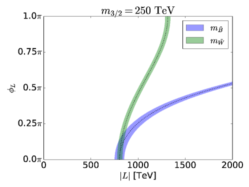
Figure 13: Contours of constant Bino and Wino masses on the $|L|$ vs. $\phi_{L}$ plane, taking $m_{3/2}=250\,\mathrm{TeV}$. The dotted lines show the true Bino and the Wino masses for Sample Point 1, while the bands show expected uncertainties due to the uncertainty in the gaugino mass determination.

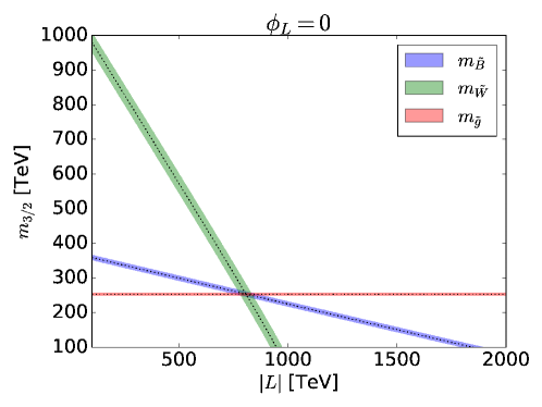
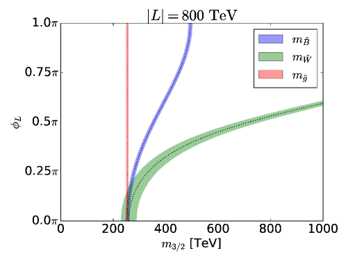
Figure 14: Contours of constant gaugino masses on the $|L|$ vs. $m_{3/2}$ plane, taking $\phi_{L}=0$. The dotted lines show the true gaugino masses for Sample Point 1, while the bands show expected uncertainties due to the uncertainty in the gaugino mass determination.

Figure 15: Contours of constant gaugino masses on the $m_{3/2}$ vs. $\phi_{L}$ plane, taking $|L|=800\,\mathrm{TeV}$. The dotted lines show the true gaugino masses for Sample Point 1, while the bands show expected uncertainties due to the uncertainty in the gaugino mass determination.

Here, we consider how well we can test the PGM prediction and how well we can determine fundamental parameters. For this purpose, we consider the parameter region consistent with observed gaugino masses, adopting Sample Point 1 as an example. To begin with, we plot contours of constant gaugino masses on the $|L|$ vs. $\phi_{L}$ plane in figure 13, with fixing $m_{3/2}=250\ {\rm GeV}$ (i.e. the true value of the gravitino mass); the dotted lines are contours of true Bino and Wino masses, while the bands show the expected uncertainties given in tables 2 and 4. Notice that the gluino mass is independent of $|L|$ and $\phi_{L}$, and is $6\ {\rm TeV}$ for $m_{3/2}=250\ {\rm GeV}$. We can estimate the uncertainties in the determination of these two parameters as $\delta|L|\sim 25\,\mathrm{TeV}$ and $\delta\phi_{L}\sim\pi/5$. In figures 15 and 15, we also show the contours of constant gaugino masses on the $|L|$ vs. $m_{3/2}$ plane and the $m_{3/2}$ vs. $\phi_{L}$ plane, respectively. In each figure, the remaining parameter ($\phi_{L}$ or $|L|$) is fixed to its input value; the dotted lines show the contours of true gaugino masses, while the bands stand for the expected uncertainty due to the uncertainties in the gaugino mass determination. Particularly from the gluino mass information, we can see that the gravitino mass $m_{3/2}$ can be determined with the accuracy of $\delta m_{3/2}\sim 5\,\mathrm{TeV}$.

Once $|L|$ is determined, it will provide information about the masses of heavier MSSM particles. One of the important purposes of high energy colliders is to understand the mass scales of unknown particles; determination of $|L|$ gives information about the mass scales of Higgsinos and heavy Higgses. From eq. (4), we can see that $|L|$ depends on $|\mu|$, $m_{A}$, and $\tan\beta$. In the PGM model, the masses of the Higgsinos and heavy Higgses are expected to be of the same order of magnitude, and hence information about $|L|$ gives a good estimate of their mass scale as $|\mu|\sim m_{A}\sim|L|/\sin 2\beta$. More precisely, we may estimate an upper bound on the mass scale below which Higgisnos or heavy Higgses, whichever lighter, should exist. Such an upper bound depends on the hierarchy between $|\mu|$ and $m_{A}$ parameterized by

$$x=\frac{m_{A}}{|\mu|}.$$ (3)

Varying $x$ within the range $x_{\rm min}\leq x\leq x_{\rm max}$, we calculate the maximal possible value of $\mbox{min}(|\mu|,m_{A})$ to derive the upper bound on the mass scale:

$$\overline{\mbox{min}}(|\mu|,m_{A})\equiv\underset{x_{\rm min}\leq x\leq x_{\rm max}}{\mbox{max}}\mbox{min}(|\mu|,m_{A}).$$ (4)

Here, $x_{\rm min}$ and $x_{\rm max}$ parameterize the possible hierarchy between $|\mu|$ and $m_{A}$, and both of them are expected to be of $O(0.1-1)$ in the PGM model. Based on eq. (4), $\overline{\mbox{min}}(|\mu|,m_{A})$ is given by

$$\overline{\mbox{min}}(|\mu|,m_{A})=\frac{|L|}{\sin 2\beta}\frac{1-x_{\rm min}^{2}}{x_{\rm min}\ln x_{\rm min}^{-2}},$$ (5)

where we consider the case of $x_{\rm min}\leq 1$.

In figure 16, we plot $\overline{\mbox{min}}(|\mu|,m_{A})$ taking the input value of $|L|$ ($=800\,\mathrm{TeV}$) of Sample Point 1. Here, we take $x_{\rm min}=0.1$, $0.3$, and $1$. The upper bound on the mass scale of Higgsinos and heavy Higgses becomes larger for a larger value of $\tan\beta$. We comment here that $\tan\beta$ is also correlated with the sfermion mass scale $M_{\mathrm{S}}$ (in particular that of stops) through the observed value of the Higgs mass. At the sfermion mass scale, the Higgs quartic coupling $\lambda$ is determined as Bernal:2007uv ; Giudice:2011cg

$$\lambda(M_{\mathrm{S}})=\frac{g_{1}^{2}(M_{\mathrm{S}})+g_{2}^{2}(M_{\mathrm{S}})}{4}\cos^{2}2\beta+\delta\lambda,$$ (6)

where $\delta\lambda$ denotes the threshold correction from sfermions and Higgsinos. After taking into account the renormalization group effects, the value of $\lambda$ at the electroweak scale determines the Higgs mass Buttazzo:2013uya . In figure 16, we also show $M_{\mathrm{S}}$ as a function of $\tan\beta$ to realize the observed Higgs mass of $m_{h}=125.18\,\mathrm{GeV}$ Tanabashi:2018oca . As is well known, $M_{\mathrm{S}}$ becomes larger as $\tan\beta$ becomes smaller; this is due to the cancellation between the $\tan\beta$ dependence of the tree-level contribution to $\lambda$ and the renormalization group effect on $\lambda$. Resultantly, $|L|/\sin 2\beta$ and $M_{\mathrm{S}}$ have opposite correlation with $\tan\beta$. Then, two lines in figure 16 intersect with each other at the mass scale $\sim 10^{3}\,\mathrm{TeV}$. This implies that, with the determination of $|L|$, we will acquire the mass scale below or at which a new particle (i.e. Higgsinos, heavy Higgs bosons, or sfermions) should exist. Notice that, since the qualitative behaviours of these two lines always hold, such a mass scale can be always acquired with the determination of $|L|$.

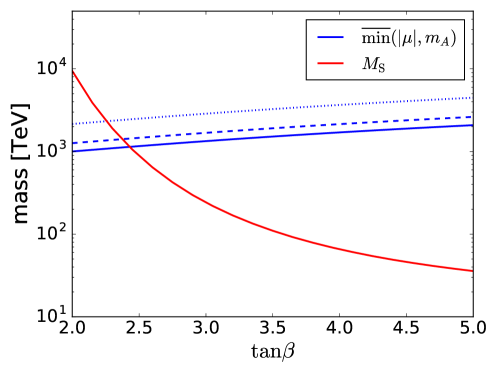
Figure 16: $\overline{\mbox{min}}(|\mu|,m_{A})$ as a function of $\tan\beta$ taking the input value of $|L|$ ($=800\,\mathrm{TeV}$) of Sample Point 1 (blue lines). Solid, dashed, and dotted blue lines correspond to $x_{\rm min}=1$, $0.3$, and $0.1$, respectively. $M_{\mathrm{S}}$ is also shown in the red line.

6 Conclusions and discussion

In this paper, we have discussed a prospect of the study of a SUSY model at the FCC. We have concentrated on the so-called PGM model of SUSY breaking, in which scalars in the MSSM sector have masses of $O(100)\ {\rm TeV}$ while gauginos are within the kinematical reach of the FCC, and have studied the SUSY signals at the FCC. We have paid particular attention to the case where Wino is lighter than other gauginos and neutral Wino is the LSP. In such a case, the charged Wino has its lifetime of $c\tau_{\tilde{W}^{\pm}}\simeq 5.75\ {\rm cm}$ and can give unique disappearing tracks in the inner pixel detector. The charged Wino tracks can be used not only for the reduction of standard-model backgrounds but also for the reconstruction of SUSY events.

In the model of our interest, gauginos are the only SUSY particles that are accessible with the FCC. We have proposed procedures to determine their masses.

• Once two charged Wino tracks are identified, the Wino mass can be determined by combining velocity and momentum information of each Wino; here, the velocity can be determined by using the time information from the pixel detector while the momentum of the Wino is determined by using the conservation of the transverse momentum.

• The Bino mass can be determined by using the fact that the decay 1 process $\tilde{B}\rightarrow\tilde{W}^{\pm}W^{\mp}$ has sizeable branching ratio. In particular, at the FCC, the $W$-boson produced by the Bino decay can be highly boosted, and hence hadrons from the decay of $W$-boson may result in a single fat jet with the jet mass close to the $W$-boson mass. Studying the invariant mass of the system consisting of a charged Wino (observed as a disappearing track) and a fat $W$-jet, information about the Bino mass can be obtained.

• For the gluino mass determination, we use the fact that, requiring two charged Wino tracks in the event, we can observe all the decay products of gluinos, i.e. charged Winos and jets, assuming that all the decay products of gluinos are hadrons and Winos. We have discussed the possibility to determine the gluino mass using the hemisphere analysis to recombine decay products of each gluino. A distribution of the invariant masses of hemispheres gives information about the gluino mass.

We emphasize here that there are several assumptions made in this paper. Charged Wino tracks can be reconstructed with high efficiency, even though the transverse flight length is as short as $\sim 10\ {\rm cm}$. The velocity of charged Wino can be determined with the accuracy of $O(1)\ \%$, which depends on the hit-level time resolution of the pixel detector. For the background, we consider only fake disappearing tracks because they are expected to be dominant in high pile-up conditions, but it should be kept in mind that physical background due to particle scattering also exists to some extent. The gaugino mass determination will be affected by contributions from additional energies deposited in jets such as pile-ups, but such contributions could be sufficiently suppressed by using pile-up mitigation techniques, as indicated in ref. FCChh_CDR . The event selections that we have used in this paper are sufficient to characterize the properties of signal events while they might need to be altered if more realistic background is considered. All these conditions may affect the gaugino mass determination, and the details in realistic situation will be studied in the future.

The proposed method in this paper is contingent on the existence of an inner tracking detector with the hit-time resolution of $O(10)\ {\rm ps}$. For understanding this SUSY model with the proposed method, technology of the timing-capable sensors in a high radiation environment has be developed.

Once three gaugino masses are known, the result can be used to understand the underlying theory of SUSY breaking and to reconstruct fundamental parameters behind the gaugino masses. In the PGM model of our interest, gaugino masses depend on three parameters, i.e.,$m_{3/2}$, $|L|$, and $\phi_{L}$. Even though there are three free parameters for three gaugino masses, there exists a non-trivial constraint as shown in eq. (2). Thus, by checking if the observed gaugino masses are in agreement with the PGM relation, we can test the PGM model as a model of SUSY breaking. Simultaneously, we can determine the fundamental parameters $m_{3/2}$, $|L|$, and $\phi_{L}$. In particular, with the determination of $|L|$, information about the masses of Higgsinos and heavy Higgses are obtained (see eq  (4)). Furthermore, understanding of the gravitino mass $m_{3/2}$ will shed light on the mechanism of SUSY breaking. Determination of the gravitino mass has implications also for cosmology. For example, once the gravitino mass is known, an upper bound on the reheating temperature after inflation can be precisely determined in order not to spoil the success of big-bang nucleosynthesis. For the understanding of the thermal history of the universe, such an upper bound gives very important information.

In summary, we have demonstrated that the FCC can play crucial roles in the understanding of physics beyond the standard model. We have considered only the PGM model of SUSY breaking, and the importance of the FCC will become clearer with the studies of other cases.

- (1) M. L. Mangano et al., Physics at a 100 TeV pp Collider: Standard Model Processes, CERN Yellow Report (2017) no.3, 1 [arXiv:1607.01831 [hep-ph]].
- (2) R. Contino et al., Physics at a 100 TeV pp collider: Higgs and EW symmetry breaking studies, CERN Yellow Report (2017) no.3, 255 [arXiv:1606.09408 [hep-ph]].
- (3) T. Golling et al., Physics at a 100 TeV pp collider: beyond the Standard Model phenomena, CERN Yellow Report (2017) no.3, 441 [arXiv:1606.00947 [hep-ph]].
- (4) M. Ibe, T. Moroi and T. T. Yanagida, Possible Signals of Wino LSP at the Large Hadron Collider, Phys. Lett. B 644 (2007) 355 [hep-ph/0610277].
- (5) M. Ibe and T. T. Yanagida, The Lightest Higgs Boson Mass in Pure Gravity Mediation Model, Phys. Lett. B 709 (2012) 374 [arXiv:1112.2462 [hep-ph]].
- (6) N. Arkani-Hamed, A. Gupta, D. E. Kaplan, N. Weiner and T. Zorawski, Simply Unnatural Supersymmetry, arXiv:1212.6971 [hep-ph].
- (7) L. Randall and R. Sundrum, Out of this world supersymmetry breaking, Nucl. Phys. B 557 (1999) 79 [hep-th/9810155].
- (8) G. F. Giudice, M. A. Luty, H. Murayama and R. Rattazzi, Gaugino mass without singlets, JHEP 9812 (1998) 027 [hep-ph/9810442].
- (9) N. Arkani-Hamed, A. Delgado and G. F. Giudice, The Well-tempered neutralino, Nucl. Phys. B 741 (2006) 108 [hep-ph/0601041].
- (10) H. C. Cheng, B. A. Dobrescu and K. T. Matchev, Generic and chiral extensions of the supersymmetric standard model, Nucl. Phys. B 543 (1999) 47 [hep-ph/9811316].
- (11) J. L. Feng, T. Moroi, L. Randall, M. Strassler and S. f. Su, Discovering supersymmetry at the Tevatron in wino LSP scenarios, Phys. Rev. Lett. 83 (1999) 1731 [hep-ph/9904250].
- (12) M. Aaboud et al. [ATLAS collaboration], Search for long-lived charginos based on a disappearing-track signature in collisions at =13 TeV with the ATLAS detector, JHEP 06 (2018) 022 [arXiv:1712.02118 [hep-ex]].
- (13) A. M. Sirunyan et al. [CMS collaboration], Search for disappearing tracks as a signature of new long-lived particles in proton-proton collisions at =13 TeV, JHEP 08 (2018) 016 [arXiv:1804.07321 [hep-ex]].
- (14) M. Low and L.-T. Wang, Neutralino dark matter at 14 TeV and 100 TeV, JHEP 08 (2014) 161 [arXiv:1404.0682 [hep-ph]].
- (15) M. Cirelli, F. Sala and M. Taoso, Wino-like Minimal Dark Matter and future colliders, JHEP 10 (2014) 033 Erratum: JHEP 01 (2015) 041 [arXiv:1407.7058 [hep-ph]].
- (16) T. Gherghetta, G. F. Giudice and J. D. Wells, Phenomenological consequences of supersymmetry with anomaly induced masses, Nucl. Phys. B 559 (1999) 27 [hep-ph/9904378].
- (17) G. F. Giudice and A. Romanino, Split supersymmetry, Nucl. Phys. B 699 (2004) 65 Erratum: [Nucl. Phys. B 706 (2005) 487] [hep-ph/0406088].
- (18) M. Tanabashi et al. [Particle Data Group], Review of Particle Physics, Phys. Rev. D 98 (2018) no.3, 030001.
- (19) Y. Okada, M. Yamaguchi and T. Yanagida, Upper bound of the lightest Higgs boson mass in the minimal supersymmetric standard model, Prog. Theor. Phys. 85 (1991) 1.
- (20) Y. Okada, M. Yamaguchi and T. Yanagida, Renormalization group analysis on the Higgs mass in the softly broken supersymmetric standard model, Phys. Lett. B 262 (1991) 54.
- (21) J. R. Ellis, G. Ridolfi and F. Zwirner, Radiative corrections to the masses of supersymmetric Higgs bosons, Phys. Lett. B 257 (1991) 83.
- (22) J. R. Ellis, G. Ridolfi and F. Zwirner, On radiative corrections to supersymmetric Higgs boson masses and their implications for LEP searches, Phys. Lett. B 262 (1991) 477.
- (23) H. E. Haber and R. Hempfling, Can the mass of the lightest Higgs boson of the minimal supersymmetric model be larger than m(Z)?, Phys. Rev. Lett. 66 (1991) 1815.
- (24) J. Hisano, S. Matsumoto, M. Nagai, O. Saito and M. Senami, Non-perturbative effect on thermal relic abundance of dark matter, Phys. Lett. B 646 (2007) 34 [hep-ph/0610249].
- (25) T. Moroi and L. Randall, Wino cold dark matter from anomaly mediated SUSY breaking, Nucl. Phys. B 570 (2000) 455 [hep-ph/9906527].
- (26) M. Kawasaki, K. Kohri, T. Moroi and Y. Takaesu, Revisiting Big-Bang Nucleosynthesis Constraints on Long-Lived Decaying Particles, Phys. Rev. D 97 (2018) no.2, 023502 [arXiv:1709.01211 [hep-ph]].
- (27) M. Fukugita and T. Yanagida, Baryogenesis Without Grand Unification, Phys. Lett. B 174 (1986) 45.
- (28) W. Buchmuller, P. Di Bari and M. Plumacher, Leptogenesis for pedestrians, Annals Phys. 315 (2005) 305 [hep-ph/0401240].
- (29) G. F. Giudice, A. Notari, M. Raidal, A. Riotto and A. Strumia, Towards a complete theory of thermal leptogenesis in the SM and MSSM, Nucl. Phys. B 685 (2004) 89 [hep-ph/0310123].
- (30) T. Moroi and M. Nagai, Probing Supersymmetric Model with Heavy Sfermions Using Leptonic Flavor and CP Violations, Phys. Lett. B 723 (2013) 107 [arXiv:1303.0668 [hep-ph]].
- (31) D. McKeen, M. Pospelov and A. Ritz, Electric dipole moment signatures of PeV-scale superpartners, Phys. Rev. D 87 (2013) no.11, 113002 [arXiv:1303.1172 [hep-ph]].
- (32) M. Ibe, S. Matsumoto and R. Sato, Mass Splitting between Charged and Neutral Winos at Two-Loop Level, Phys. Lett. B 721 (2013) 252 [arXiv:1212.5989 [hep-ph]].
- (33) M. Saito, R. Sawada, K. Terashi and S. Asai, Discovery reach for wino and higgsino dark matter with a disappearing track signature at a 100 TeV pp collider, arXiv:1901.02987 [hep-ph].
- (34) G. Pellegrini, P. Fernández-Martínez, M. Baselga, C. Fleta, D. Flores, V Greco, S. Hidalgo, I. Mandić, G. Kramberger, D. Quirion and M. Ullan, Technology developments and first measurements of Low Gain Avalanche Detectors (LGAD) for high energy physics applications, Nucl. Instrum. Meth. A 765 (2014) 12
- (35) J. Lange, M. Carulla, E. Cavallaro, L. Chytka, P.M. Davis, D. Flores, F. Förster, S. Grinstein, S. Hidalgo, T. Komarek, G. Kramberger, I. Mandić, A. Merlos, L. Nozka, G. Pellegrini, D. Quirion and T. Sykora, Gain and time resolution of 45 m thin Low Gain Avalanche Detectors before and after irradiation up to a fluence of neq/cm2, JINST 12 (2017) P05003 [arXiv:1703.09004 [physics.ins-det]].
- (36) J. Alwall, M. Herquet, F. Maltoni, O. Mattelaer and T. Stelzer, MadGraph 5 : Going Beyond, JHEP 1106 (2011) 128 [arXiv:1106.0522 [hep-ph]].
- (37) J. Alwall et al., The automated computation of tree-level and next-to-leading order differential cross sections, and their matching to parton shower simulations, JHEP 1407 (2014) 079 [arXiv:1405.0301 [hep-ph]].
- (38) T. Sjöstrand et al., An Introduction to PYTHIA 8.2, Comput. Phys. Commun. 191 (2015) 159 [arXiv:1410.3012 [hep-ph]].
- (39) J. de Favereau et al. [DELPHES 3 Collaboration], DELPHES 3, A modular framework for fast simulation of a generic collider experiment, JHEP 1402 (2014) 057 [arXiv:1307.6346 [hep-ex]].
- (40) R. Brun and F. Rademakers, ROOT: An object oriented data analysis framework, Nucl. Instrum. Meth. A 389 (1997) 81.
- (41) S. Asai, Y. Azuma, O. Jinnouchi, T. Moroi, S. Shirai and T. T. Yanagida, Mass Measurement of the Decaying Bino at the LHC, Phys. Lett. B 672 (2009) 339 [arXiv:0807.4987 [hep-ph]].
- (42) G. L. Bayatian et al. [CMS Collaboration], CMS technical design report, volume II: Physics performance, J. Phys. G 34 (2007) no.6, 995.
- (43) M. Aaboud et al. [ATLAS Collaboration], Search for squarks and gluinos in final states with jets and missing transverse momentum using 36 fb-1 of TeV pp collision data with the ATLAS detector, Phys. Rev. D 97, no. 11, 112001 (2018).
- (44) J. Butterworth et al., PDF4LHC recommendations for LHC Run II, J. Phys. G 43, 023001 (2016).
- (45) S. Asai, T. Moroi, K. Nishihara and T. T. Yanagida, Testing the Anomaly Mediation at the LHC, Phys. Lett. B 653 (2007) 81 [arXiv:0705.3086 [hep-ph]].
- (46) N. Bernal, A. Djouadi and P. Slavich, The MSSM with heavy scalars, JHEP 0707 (2007) 016 [arXiv:0705.1496 [hep-ph]].
- (47) G. F. Giudice and A. Strumia, Probing High-Scale and Split Supersymmetry with Higgs Mass Measurements, Nucl. Phys. B 858 (2012) 63 [arXiv:1108.6077 [hep-ph]].
- (48) D. Buttazzo, G. Degrassi, P. P. Giardino, G. F. Giudice, F. Sala, A. Salvio and A. Strumia, Investigating the near-criticality of the Higgs boson, JHEP 1312 (2013) 089 [arXiv:1307.3536 [hep-ph]].
- (49) M. Benedikt et al., Future Circular Collider Study. Volume 3: The Hadron Collider (FCC-hh) Conceptual Design Report, CERN-ACC-2018-0058 (2018), Submitted to Eur. Phys. J. ST.