Floquet dynamical quantum phase transitions

Abstract

Dynamical quantum phase transitions (DQPTs) are manifested by time-domain nonanalytic behaviors of many-body systems. Introducing a quench is so far understood as a typical scenario to induce DQPTs. In this work, we discover a novel type of DQPTs, termed “Floquet DQPTs”, as intrinsic features of systems with periodic time modulation. Floquet DQPTs occur within each period of continuous driving, without the need for any quenches. In particular, in a harmonically driven spin chain model, we find analytically the existence of Floquet DQPTs in and only in a parameter regime hosting a certain nontrivial Floquet topological phase. The Floquet DQPTs are further characterized by a dynamical topological invariant defined as the winding number of the Pancharatnam geometric phase versus quasimomentum. These findings are experimentally demonstrated with a single spin in diamond. This work thus opens a door for future studies of DQPTs in connection with topological matter.

DQPTs are often associated with quantum quenches, a protocol in which parameters of a Hamiltonian are suddenly changed HeylPRL2013 ; PollmannPRE2010 . A quantum quench across an equilibrium quantum critical point may induce a DQPT. If pre-quench and post-quench systems are in topologically distinct phases, DQPTs may also be characterized by dynamical topological invariants DTOP1 ; DTOP2 ; DTOP3 . As a promising approach to classify quantum states of matter in nonequilibrium situations, DQPTs have been theoretically explored in both closed and open quantum systems at different physical dimensions DQPTRev1 ; DQPTRev2 ; ZhouArXiv2017 . Experimentally, DQPTs have been observed in trapped ions DQPTExp1 ; DQPTExp2 , cold atoms DQPTExp3 ; DQPTExp4 , superconducting qubits DQPTExp5 , nanomechanical oscillators DQPTExp6 , and photonic quantum walks DQPTExp7 ; DQPTExp8 .

To date, in most studies of DQPTs, a quantum quench acts as a trigger for initiating nonequilibrium dynamics and then exposing the underlying topological features. However, DQPTs under more general nonequilibrium manipulations are still largely unexplored SharmaPRB2016 ; PuskarovSPP2016 ; BhattacharyaPRB2017 . In particular, because the dynamics of systems under time-periodic modulations has led to fascinating discoveries like Floquet topological states Lindner2011 ; FTIRev ; LW2014 ; HoPRL2012 ; LiPRL2018 and discrete time crystals TCRev ; Yao2018 ; BomantaraPRL , it is urgent to investigate how DQPTs may occur in such Floquet systems. Along this avenue, there have been scattered studies, but still with the notion that DQPTs are best aroused by a quench to some system parameters FDQPT1 ; FDQPT2 . Here we introduce a novel class of DQPTs, termed Floquet DQPTs, which can be regarded as intrinsic features of systems with time-periodic modulations. As schematically shown in Fig. 1, the Floquet DQPTs we discovered occur within each period of a continuous driving field, without the need for any quenches. In the model investigated below, the occurrence of Floquet DQPTs and the emergence of Floquet topological phases are in the same parameter regime. We further perform a quantum simulation experiment using a single electron spin in diamond to verify our main theoretical findings.

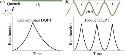
Figure 1: Comparison between (a) DQPTs following a quantum quench, and (b) Floquet DQPTs without any quenches. Here $H_{i}$ and $H_{f}$ denote the Hamiltonians before and after the quench, $H(t)$ denotes a periodically and continuously modulated Hamiltonian.

For a periodically modulated system ${\cal H}(t)={\cal H}(t+T)$ with $T$ the modulation period and $\omega=2\pi/T$ the frequency, the time-dependent Schrödinger equation yields solutions $|\Psi_{n}(t)\rangle=e^{-i\varepsilon_{n}t}|\Phi_{n}(t)\rangle$, with the Floquet mode $|\Phi_{n}(t)\rangle=|\Phi_{n}(t+T)\rangle$ and the quasienergy $\varepsilon_{n}\in[-\omega/2,\omega/2)$ HolthausFloTut . Though a Floquet mode by definition becomes parallel to itself at multiple $T$’s, it still evolves nontrivially within each driving period (hence the micromotion dynamics). More specifically, consider a periodically driven system prepared initially at a many-particle Floquet state $|\Psi_{n}(0)\rangle$, which is the product state of Floquet modes $|\varphi_{n}(0)\rangle$ filling the quasienergy band $n$. The return amplitude of the system at $t>0$ is then ${\cal G}_{n}(t)\equiv\langle\Psi_{n}(0)|\Psi_{n}(t)\rangle$. In the thermodynamic limit, the rate function is defined as

$$g_{n}(t)\equiv-\lim_{N\rightarrow\infty}\frac{1}{N}\ln|{\cal G}_{n}(t)|^{2},$$ (1)

where $|{\cal G}_{n}(t)|^{2}$ is the return probability, and $N$ is the number of degrees of freedom, such as the number of lattice sites in a chain. The rate function $g_{n}(t)$ plays the role of a dynamical free energy HeylPRL2013 ; SM , which is periodic in time with period $T$. Now if there exists a critical time $t_{c}$, at which $|\Psi_{n}(t_{c})\rangle$ is orthogonal to $|\Psi_{n}(0)\rangle$, one finds ${\cal G}_{n}(t_{c})=0$. Then $g_{n}(t)$ as defined in Eq. (1) or its time derivatives becomes nonanalytic at $t=t_{c}$.

We now focus on a harmonically driven spin chain described by $H(t)=\sum_{n}[(\delta_{1}-\Omega\sin\omega t)s_{n}^{x}s_{n+1}^{x}+(\delta_{1}+\Omega\sin\omega t)s_{n}^{y}s_{n+1}^{y}-\delta_{2}s_{n}^{z}-\Omega\cos\omega t(s_{n}^{x}s_{n+1}^{y}+s_{n}^{y}s_{n+1}^{x})]$, where $s_{n}^{x,y,z}$ are quantum spin-$1/2$ variables localized at site $n$ of the chain; $\delta_{1}$, $\delta_{2}$, and $\Omega$ are system parameters. The associated Bloch Hamiltonian is found to be SM

$$H(k,t)=\frac{\Omega\sin k}{2}[\cos(\omega t)\sigma_{x}+\sin(\omega t)\sigma_{y}]+\frac{\delta_{1}\cos k+\delta_{2}}{2}\sigma_{z}.$$ (2)

where $k$ is the quasimomentum. The dynamics governed by $H(k,t)$ is analytically solvable and has been already experimentally realized in other quantum simulation studies GTPExp . The bulk dynamics of the system can be solved because each occupied $k$ component of the system evolves independently. The Floquet state at each $k$ is given by $|\psi_{\pm}(k,t)\rangle=e^{-iE_{\pm}(k)t}U_{R}(t)|\varphi_{\pm}(k,0)\rangle$. Here $E_{\pm}(k)$ are quasienergy dispersions of two Floquet bands with the Floquet modes $|\varphi_{\pm}(k,t)\rangle=U_{R}(t)|\varphi_{\pm}(k,0)\rangle$, $U_{R}(t)={\rm diag}(1,e^{i\omega t})$ is responsible for the micromotion dynamics, and $|\varphi_{\pm}(k,0)\rangle$ are the eigenstates of the static Hamiltonian $H_{F}(k)=\Omega\sin k~{}\sigma_{x}/2+(\delta_{1}\cos k+\delta_{2}-\omega)\sigma_{z}/2$ SM .

The micromotion dynamics arising from $U_{R}(t)$ is the rotation around the $z$ axis (with frequency $\omega$) on the Bloch sphere SM . If there exists $k=k_{c}$ such that $|\varphi_{\pm}(k,0)\rangle$ lies in the $x$-$y$ plane, then the micromotion dynamics can always rotate this initial state to a state pointing at exactly the opposite direction at $t=t_{c}=(2m-1)T/2$ for $m\in\mathbb{Z}^{+}$. That is, at $t=t_{c}$ the time-evolving state at this quasimomentum becomes orthogonal to its initial state. Assuming that the collective initial state of the system fills one of the Floquet bands $|\Psi_{\alpha}(0)\rangle=\prod_{k>0}|\psi_{\alpha}(k,0)\rangle=\prod_{k>0}|\varphi_{\alpha}(k,0)\rangle$ with band indices $\alpha=+$ or $-$. At a later time $t$, the return amplitude of the system is given by ${\cal G}_{\alpha}(t)=\prod_{k>0}G_{\alpha}(k,t)$, with $G_{\alpha}(k,t)=\langle\psi_{\alpha}(k,0)|\psi_{\alpha}(k,t)\rangle$. It can be shown that, under the condition

$$\left|\omega-\delta_{2}\right|\leq\left|\delta_{1}\right|,$$ (3)

there exists a critical momentum $k_{c}$ with $\delta_{1}\cos k_{c}=\omega-\delta_{2}$, such that $|\varphi_{\alpha}(k_{c},0)\rangle$ lies in the $x$-$y$ plane SM and consequently $G_{\alpha}(k_{c},t)=0$. Under the condition (3), the rate function $g_{\alpha}(t)=-\int dk\ln|G_{\alpha}(k,t)|^{2}$ becomes non-analytic at each critical time $t_{c}$. It can be also shown that there exists a topological order parameter given by the winding number of the geometric phase over the Brillouin zone, namely,

$${\nu_{\alpha}}(t)=\int_{0}^{\pi}\frac{{dk}}{{2\pi}}\frac{\partial\phi_{\alpha}^{\rm{geo}}(k)}{\partial k},$$ (4)

where $\phi_{\alpha}^{{\rm{geo}}}(k)$ is the Pancharatnam geometric phase acquired during the evolution of a Floquet state at quasimomentum $k$ SM . When time passes the critical time of a Floquet DQPT, $\nu_{\alpha}(t)$ makes a quantized jump. The winding number $\nu_{\alpha}(t)$ as a dynamical topological invariant thus reflects the topological nature of Floquet DQPTs identified in the spin chain model here.

Before proceeding to experiment, three traits of Floquet DQPTs deserve to be highlighted. Firstly, no quantum quench from one equilibrium phase to another is required in our proposal, as the continuous driving field suffices to generate non-analyticities in the time domain. Secondly, the Floquet DQPTs introduced in this work repeat periodically in time, whereas the DQPTs following a single quench are usually visible only in transient time windows due to the decay of the rate function. Floquet DQPTs are therefore more accessible to experiments. Thirdly, precisely under the same condition as in (3), our spin chain model is found to reside in a nontrivial “chiral-symmetric” Floquet topological phase SM , as featured by two winding numbers defined with the one-period evolution operator in two chiral-symmetric time frames AsbothPRB2013 . These two winding numbers can be used to predict topological edge states under open boundary conditions. As such, the Floquet DQPTs reported here not only provide an indirect probe to study these intriguing Floquet topological phases, but also suggest a remarkable connection between jumps in the dynamical topological invariant ${\nu_{\alpha}}(t)$ and the emergence of a Floquet topological phase SM .

A negatively charged nitrogen-vacancy (NV) center in diamond is used in our experiment to simulate $H(k,t)$ GTPExp , the many-body Hamiltonian in its quasimomentum representation. As shown in Fig. 2(a), the NV center is composed of one substitutional nitrogen atom and an adjacent vacancy Doherty ; Schirhagl ; Prawer ; Wrachtrup . In our experiment, an external static magnetic field around $510$ G is parallel to the NV symmetry axis, which enables both the NV electron spin and the host ¹⁴N nuclear spin to be polarized by optical excitation Jacques ; Sar . The Hamiltonian of the electronic ground state of the NV center with a static magnetic field $B$ applied along the NV axis (also the $z$ axis) is $H_{\rm{NV}}=DS_{z}^{2}+\gamma BS_{z}$, where $S_{z}$ is the angular momentum operator for spin-1, $D=2\pi\times 2870$ MHz is the zero-field splitting, and $\gamma=2\pi\times 2.8$ MHz/G is the gyromagnetic ratio of the NV electron. As illustrated in Fig. 2(b), microwaves generated by an arbitrary waveform generator drives the transition between the electronic levels $\left|{{m_{s}}=0}\right\rangle$ and $\left|{{m_{s}}=-1}\right\rangle$ which compose a qubit. The level $\left|{{m_{s}}=1}\right\rangle$ remains idle due to large detuning. The probability in $\left|{{m_{s}}=0}\right\rangle$ can be read out via fluorescence detection during optical excitation. All the optical procedures are performed on a home-built confocal microscope, and a solid immersion lens is etched on the diamond above the NV center to enhance the fluorescence collection Robledo ; Rong .

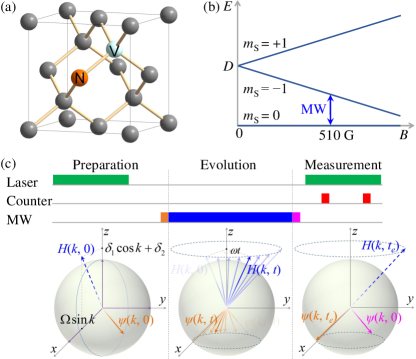
Figure 2: Experimental system and method. (a) NV center in diamond. (b) Electronic ground state of a negatively charged NV center. The energy splitting depends on the magnetic field which is parallel to the NV axis in this experiment. The two levels $\left|{{m_{s}}=0}\right\rangle$ and $\left|{{m_{s}}=-1}\right\rangle$ are encoded as a qubit which is manipulated by microwaves (MW). (c) Pulse sequence for qubit control and measurement. In the pulse sequence illustrated here, the microwave pulse in the measurement section aims for acquiring the return probability. The Bloch vector of the quantum state and the direction of the rotating field are shown below the pulse sequence.

In our experiment, the evolution at different $k$ is performed separately in different experimental runs. The pulse sequence for each $k$ is sketched in Fig. 2(c). At first, the qubit is polarized to the state $|0\rangle$ by a laser pulse [green bar in the preparation section in Fig. 2(c)]. A resonant microwave pulse [orange bar in Fig. 2(c)] is then applied to prepared the initial state as $|\varphi_{-}(k,0)\rangle$, which occupies the lower quasienergy band. The Bloch vector of this initial state is along the direction $\bm{n}(k,0)=\left(-\Omega\sin k,0,\omega-{\delta_{1}}\cos k-{\delta_{2}}\right)$. The parameters adopted in our experiment are $\Omega=2\pi\times 10$ MHz, $\omega=\delta_{1}=2\pi\times 5$ MHz, and $\delta_{2}=\pm 2\pi\times 5$ MHz. For $\delta_{2}=2\pi\times 5$ MHz, the prepared initial state lies in the $x$-$y$ plane for $k_{c}=\pi/2$. This is not the case for any $k$ if $\delta_{2}=-2\pi\times 5$ MHz, thus excluding DQPTs.

Upon initial-state preparation, the qubit is left to evolve under $H(k,t)$, namely, in the presence of a field with the transverse component $\Omega\sin k$ and the longitudinal component ${\delta_{1}}\cos k+{\delta_{2}}$. The field is rotated around the $z$ axis with the angular frequency $\omega$, which is implemented by applying a microwave pulse starting from $t=0$, as depicted by the blue bar in Fig. 2(c).

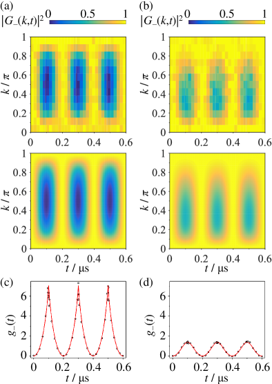
Figure 3: Return probabilities and rate functions. (a)(b) Return probabilities for $\delta_{2}=2\pi\times 5$ MHz and $-2\pi\times 5$ MHz, respectively. Experimental data are shown in the upper panels and theoretical results are presented in the lower panels. All panels in (a) and (b) share the same color bar. The associated rate functions are shown in panels (c) and (d), with black circles and red curves representing experimental data and theoretical values.

The evolution governed by $H(k,t)$ lasts for some duration $t_{e}$, and then the return probability $|G_{-}(k,t_{e})|^{2}=|\langle\psi_{-}(k,0)|\psi_{-}(k,t_{e})\rangle|^{2}$ needs to be measured. The measurement procedure begins with a resonant microwave pulse [the magenta bar in Fig. 2(c)], which steers the direction of $\bm{n}(k,0)$ to the $+z$ direction. It is followed by a laser pulse [green bar in the measurement section of Fig. 2(c)] together with fluorescence detection. The later is collected via two counting windows represented by the red bars in Fig. 2(c), with the first recording the signal while the second recording the reference SM . The fluorescence collection amounts to the measurement of the probability in $|0\rangle$, and this effect combined with the last microwave pulse is equivalent to the measurement of $|G_{-}(k,t_{\rm e})|^{2}$.

The above sequence is performed for a series of $t_{e}$ within 0.6 $\mu$s, and is iterated five hundred thousand times to obtain the expectation value. One can then get $|G_{-}(k,t)|^{2}$ as a function of $t$. This procedure is repeated for different values of $k\in[0,\pi]$. The experimental data with $\delta_{2}=2\pi\times 5$ MHz and $-2\pi\times 5$ MHz are illustrated in the upper panels of Fig. 3(a) and Fig. 3(b), respectively. The experimental results agree with the theoretical ones which are shown in the lower panels. The results in Fig. 3(a) confirm that, in the case of $\delta_{2}=2\pi\times 5$ MHz where the DQPT condition in Eq. (3) is satisfied, the return probability at the critical momentum $k_{c}=\pi/2$ vanishes at the critical times such as $t=0.1\ \rm{\mu s}$, $0.3\ \rm{\mu s}$, and $0.5\ \rm{\mu s}$. The DQPT condition in Eq. (3) is not satisfied in the case of $\delta_{2}=-2\pi\times 5$ MHz. The return probability never vanishes in this case as confirmed by the results in Fig. 3(b).

Numerical integration over $k$ based on the negative logarithm of these experimental data yields the experimental values of the rate function $g_{-}(t)$. Under the condition in Eq. (3) for Floquet DQPTs, the rate function behaves non-analytically at critical times, as shown by the kinks in Fig. 3(c) noerrorbar . By contrast, the rate function $g_{-}(t)$ stretches smoothly over time without non-analyticity when the DQPT condition is not satisfied, as shown in Fig. 3(d). This further demonstrates that Floquet DQPTs can be observed through the rate function.

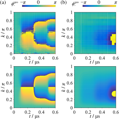
Figure 4: Measured geometric phases versus system parameter $k$ and time $t$ for (a) $\delta_{2}=2\pi\times 5$ MHz and (b) $\delta_{2}=-2\pi\times 5$ MHz. The bottom two panels represent theoretical results for the sake of comparison. In left panels, a change in the net jumps of the geometric phase along the $k$ dimension depicts a change in a dynamical topological invariant, thus signifying DQPTs at $t=0.1\ \rm{\mu s}$, $0.3\ \rm{\mu s}$, and $0.5\ \rm{\mu s}$. No such behavior is found in right panels.

In order to investigate the topological character of Floquet DQPTs, we next extract the Pancharatnam geometric phase of the time-evolving state from the expectation values of $\sigma_{x}$, $\sigma_{y}$, and $\sigma_{z}$ measured in our experiment SM . The pulse sequence for measuring these expectation values is similar to that in Fig. 2(c) except for the last microwave pulse. This resonant microwave pulse rotate the direction of $+x$ or $+y$ to $+z$ for the measurement of $\sigma_{x}$ or $\sigma_{y}$, respectively. The pulse is not needed for the measurement of $\sigma_{z}$. The experimental and theoretical values of the geometric phases for $\delta_{2}=2\pi\times 5$ MHz and $-2\pi\times 5$ MHz are illustrated in Fig. 4(a) and (b). Geometric phases with $2\pi$ difference are equivalent and we have thus set them in the range from $-\pi$ to $\pi$. The net discontinuous jump of the geometric phase along the $k$ dimension is a signature of the winding of the geometric phase with quasimomentum. The number of winding then yields $\nu_{-}(t)$ defined in Eq. (4) as a dynamical topological order parameter. In the case of Fig. 4(a) with Floquet DQPTs, the measured geometric phases manifest a jump from $-\pi$ to $\pi$ at the first critical time $t=0.1\ \rm{\mu s}$. The number of net jumps increases by one once a new critical time is passed, in particular at $t=0.3\ \rm{\mu s}$ and $t=0.5\ \rm{\mu s}$. Therefore, $\nu_{-}(t)$ increases from one at $t=0.1\ \rm{\mu s}$ to three at $t=0.5\ \rm{\mu s}$. By contrast, in the case of Fig. 4(b) where the DQPT condition in Eq. (3) is not satisfied and hence there are no DQPTs, the measured geometric phases has no net jumps along the $k$ dimension. Even when there is a discontinuous jump from $-\pi$ to $\pi$, it is cancelled by a reversed jump from $\pi$ to $-\pi$, resulting in no change in $\nu_{-}(t)$. Some noisy but insignificant patterns in the experimental results are mainly due to the imperfection of the microwave pulses. Nevertheless, even in the presence of such experimental errors, all the principal characteristics of Floquet DQPTs in connection with jumps in the dynamical topological order parameter have been clearly demonstrated.

In conclusion, we have discovered and experimentally demonstrated a new class of DQPTs as intrinsic features of quantum systems subject to smooth and periodic time modulations. Floquet DQPTs here are found to have two-fold topological nature. Firstly, their occurrence leads to jumps in a dynamical topological invariant. Secondly, the system parameters yielding Floquet DQPTs lie in a regime accommodating topologically nontrivial Floquet phases. Our work thus opens a door for future studies of DQPTs in connection with topological matter.

I I. Theory

In this supplementary note, we present in detail our theory of Floquet dynamical quantum phase transitions (DQPTs). We first briefly review the basics of conventional DQPTs and Floquet theory. Following that, we introduce our definition of Floquet DQPTs and discuss its general features. To demonstrate these features, we study the periodically driven spin chain model whose Hamiltonian in thermodynamic limit can be mapped to a qubit in a rotating field. We further solve this driven qubit model analytically and describe its Floquet DQPTs by (i) the Fisher zeros of the Loschmidt (return) amplitude, (ii) the rate function of Loschmidt echo (return probability), (iii) the pattern of a non-adiabatic, non-cyclic geometric phase, and (iv) a dynamical topological winding number. We also reveal the relation between Floquet DQPTs found in our model and its underlying Floquet topological phases. Finally, we illustrate numerically our theoretical predictions in three examples.

I.1 A. Elements of DQPTs

In this section, we briefly review the definition of DQPTs for quenched evolutions. According to Ref. HeylPRL2013 , a DQPT means that the time derivative of certain observable at a given order shows a jump or a singularity in time. It is therefore a real-time non-analytic signature in dynamics. The central quantity in the description of DQPTs is the return amplitude, defined as

$${\cal G}(t)=\langle\Psi_{i}|e^{-it{\cal H}_{f}}|\Psi_{i}\rangle,$$ (S1)

where $|\Psi_{i}\rangle$ is the initial state of the system, usually chosen to be the ground state of some many-body Hamiltonian ${\cal H}_{i}$, and ${\cal H}_{f}$ is the Hamiltonian governing the evolution of the system after the initial time $t=0$. A nonequilibrium dynamical process is generated if $[{\cal H}_{i},{\cal H}_{f}]\neq 0$, which can be realized by performing a quantum quench from ${\cal H}_{i}$ to ${\cal H}_{f}$ at $t=0$.

Formally, ${\cal G}(t)$ mimics the so-called boundary partition function in equilibrium statistical mechanics, which can be seen by rotating the time $t$ to the complex plane ($it\rightarrow z=\tau+it\in\mathbb{C}$), yielding ${\cal G}(z)=\langle\Psi_{i}|e^{-z{\cal H}_{f}}|\Psi_{i}\rangle$ DQPTRev1 . The zeros of ${\cal G}(z)$ are called Fisher zeros. They form a dense set in thermodynamic limit. A real-time Fisher zero of ${\cal G}(z)$ appears when this set crosses the imaginary time axis at some critical time $t=t_{c}$, where the rate function of return probability,

$$g(t)\equiv-\lim_{N\rightarrow\infty}\frac{1}{N}\ln|{\cal G}(t)|^{2},$$ (S2)

or its time derivative becomes non-analytic as a function of time. Here $N$ is the number of degrees of freedom of the system. Mathematically, this is closely related to the microscopic Lee-Yang theory of phase transitions. Therefore ${\cal G}(t)$ and $g(t)$ are sometimes called dynamical partition function and dynamical free energy, respectively, whereas $t_{c}$ is called the critical time of a DQPT, analogous to the critical temperature of a thermal phase transition. Theoretical studies have shown that DQPTs usually happen in dynamics following a quench across the equilibrium quantum phase transition point of the prequench Hamiltonian DQPTRev1 . Experimentally, DQPTs characterized by kinks in return rates at critical times were first observed in a one-dimensional chain of $10$ trapped ions DQPTExp1 .

I.2 B. Elements of Floquet theory

In this section, we recap some basics of Floquet theory HolthausFloTut that will be used in this study. A Floquet system is described by a time periodic Hamiltonian ${\cal H}(t)={\cal H}(t+T)$, where $T$ is the driving period and $\omega=2\pi/T$ is the driving frequency. A complete set of solutions of the time-dependent Schrödinger equation is given by the Floquet states $\{|\Psi_{n}(t)\rangle\}$, with each of them satisfying (take $\hbar=1$)

$$i\frac{d}{dt}|\Psi_{n}(t)\rangle={\cal H}(t)|\Psi_{n}(t)\rangle.$$ (S3)

The Floquet state $|\Psi_{n}(t)\rangle$ can be further decomposed as $|\Psi_{n}(t)\rangle=e^{-i\varepsilon_{n}t}|\Phi_{n}(t)\rangle$, where $\varepsilon_{n}\in[-\omega/2,\omega/2)$ is called the quasienergy and $|\Phi_{n}(t)\rangle$ is called the Floquet mode. A Floquet mode is time periodic, i.e., $|\Phi_{n}(t)\rangle=|\Phi_{n}(t+T)\rangle$. All such Floquet modes form an orthonormal, complete set at any time $t$, i.e.,

$$\sum_{\ell}|\Phi_{n}(t)\rangle\langle\Phi_{n}(t)|=1,\qquad\langle\Phi_{\ell}(t)|\Phi_{n}(t)\rangle=\delta_{\ell n}.$$ (S4)

In terms of the quasienergies and Floquet modes, the time evolution operator of the system from an initial time $0$ to a later time $t$ can be expressed as

$${\cal U}(t)=\sum_{\ell}e^{-i\varepsilon_{\ell}t}|\Phi_{\ell}(t)\rangle\langle\Phi_{\ell}(0)|.$$ (S5)

It is not hard to verify that $U(0)=1$ and

$$i\frac{d}{dt}{\cal U}(t)=\sum_{\ell}e^{-i\varepsilon_{\ell}t}\left(\varepsilon_{\ell}+i\frac{d}{dt}\right)|\Phi_{\ell}(t)\rangle\langle\Phi_{\ell}(0)|=\sum_{\ell}e^{-i\varepsilon_{\ell}t}H(t)|\Phi_{\ell}(t)\rangle\langle\Phi_{\ell}(0)|=H(t){\cal U}(t),$$ (S6)

as expected. One may further write a Floquet mode $|\Phi_{n}(t)\rangle$ as $|\Phi_{n}(t)\rangle=P(t)|\Phi_{n}(0)\rangle$, where $P(t)=P(t+T)$ is called the micromotion operator.

I.3 C. Floquet DQPTs — definition and properties

We will introduce our definition of Floquet DQPTs in this section. Consider a system described by a time-periodic Hamiltonian ${\cal H}(t)$, which is prepared initially ($t=0$) at an $N$-particle Floquet state $|\Psi_{n}(0)\rangle$, given by Floquet modes $|\Phi_{n}(0)\rangle$ filling the quasienergy band $n$. At a later time $t$, the return amplitude of the system to its initial state is given by

$${\cal G}_{n}(t)=\langle\Psi_{n}(0)|{\cal U}(t)|\Psi_{n}(0)\rangle.$$ (S7)

The time evolution operator ${\cal U}(t)={\cal T}e^{-i\int_{0}^{t}ds{\cal H}(s)}$, where ${\cal T}$ denotes the time ordering operator. In terms of quasienergies and Floquet modes, ${\cal U}(t)$ can be expressed as Eq. (S5). Then we can write the return amplitude for each Floquet mode involved in the dynamcis as

$${\cal G}_{n}(t)=e^{-i\varepsilon_{n}t}\langle\Phi_{n}(0)|\Phi_{n}(t)\rangle.$$ (S8)

The corresponding return probability to the initial state is given by

$$|{\cal G}_{n}(t)|^{2}=|\langle\Phi_{n}(0)|\Phi_{n}(t)\rangle|^{2}=|\langle\Phi_{n}(0)|P(t)|\Phi_{n}(0)\rangle|^{2},$$ (S9)

with the micromotion operator $P(t)$ introduced in the previous section. In thermodynamic limit, the rate function of return probability reads

$$g_{n}(t)=-\lim_{N\rightarrow\infty}\frac{1}{N}\ln|{\cal G}_{n}(t)|^{2}=-\lim_{N\rightarrow\infty}\frac{1}{N}\sum_{\rm{occ.}}\ln|{\cal G}_{n}(t)|^{2},$$ (S10)

where $N$ is the number of degrees of freedom (e.g., number of particles) of the system and the summation $\sum_{\rm{occ.}}$ is taken over the $N$ occupied states. In our construction of Floquet DQPTs, $g_{n}(t)$ plays the role of a dynamical free energy. If there exists a critical time $t_{c}$, at which $|\Phi_{n}(t_{c})\rangle$ is orthogonal to the initial state $|\Phi_{n}(0)\rangle$, ${\cal G}(t_{c})$ will vanishes. Then $g_{n}(t)$ as defined in Eq. (S10) or its time derivatives will become non-analytic as a function of time $t$. We refer to this as a Floquet DQPT. From Eq. (S9), one may interpret a Floquet DQPT as originated from the interplay between the stroboscopic nature of the system encoded in its Floquet mode $|\Phi_{n}(0)\rangle$, and the micromotion within a driving period described by $P(t)$.

Compared with the DQPTs following a sudden quench HeylPRL2013 , a notable difference of Floquet DQPTs is that they happen in time periodically. This is not hard to see from Eq. (S10), since

$$g_{n}(t+T)= -\lim_{N\rightarrow\infty}\frac{1}{N}\ln|{\cal G}_{n}(t+T)|^{2}=-\lim_{N\rightarrow\infty}\frac{1}{N}\sum_{\rm{occ.}}\ln|\langle\Phi_{n}(0)|P(t+T)|\Phi_{n}(0)\rangle|^{2}$$

$$= -\lim_{N\rightarrow\infty}\frac{1}{N}\sum_{\rm{occ.}}\ln|\langle\Phi_{n}(0)|P(t)|\Phi_{n}(0)\rangle|^{2}=g_{n}(t).$$ (S11)

Therefore, if $t_{c}$ is a critical time, then $t_{c}+\nu T$ is also a critical time for any $\nu\in\mathbb{Z}$, with $g_{n}(t)$ taking equal values at these critical times. Practically, this means that Floquet DQPTs will not just happen in a transient time scale as the DQPTs following a single quench, but will be observable with equal strength in a much wider time window thanks to the periodic drivings applied to the system. Furthermore, the driving fields also yield more freedom to control Floquet DQPTs in the system.

In the following sections of this theoretical part, we will study an analytically solvable driven spin chain model as described in the main text, which possesses the defining features of Floquet DQPTs. We will further map the Hamiltonian of this driven spin chain to the parameter space of a qubit in a rotating magnetic field, which allows us to develop a systematic description of Floquet DQPTs in this system (see Table 1 for an outline).

Concepts	Expressions	Annotations
Spin chain	${\cal H}(t)=\sum_{n}\left\{[\delta_{1}-\Omega\sin(\omega t)]s_{n}^{x}s_{n+1}^{x}+[\delta_{1}+\Omega\sin(\omega t)]s_{n}^{y}s_{n+1}^{y}\right\}$	${\cal H}(t)={\cal H}(t+T)$
Hamiltonian	$-\delta_{2}\sum_{n}s_{n}^{z}-\Omega\cos(\omega t)\sum_{n}\left(s_{n}^{x}s_{n+1}^{y}+s_{n}^{y}s_{n+1}^{x}\right)$	$T=2\pi/\omega$
Lattice	${\cal H}(t)=\sum_{k\in{\rm BZ}}\Psi_{k}^{\dagger}H(k,t)\Psi_{k}$	Obtained from the spin chain Hamiltonian through
Hamiltonian	$H(k,t)=\Omega\sin k[\cos(\omega t)\sigma_{x}+\sin(\omega t)\sigma_{y}]/2+(\delta_{1}\cos k+\delta_{2})\sigma_{z}/2$	Jordan-Wigner and Fourier transforms,
Bloch Hamiltonian	$H_{F}(k)\equiv U_{R}^{\dagger}(t)\left[H(k,t)-i\frac{d}{dt}\right]U_{R}(t)$	Rotation $U_{R}(t)=\begin{pmatrix}1&0\\ 0&e^{i\omega t}\end{pmatrix}=U_{R}(t+T)$
in rotating frame
Quasienergies and	$E_{\pm}(k)={\omega}/{2}\pm\sqrt{h_{xy}^{2}(k)+\left[h_{z}(k)-{\omega}/{2}\right]^{2}}$	$E_{\pm}(k)$ and $|\varphi_{\pm}(k,0)\rangle$ are eigenvalues
Floquet eigenstates	$|\psi_{\pm}(k,t)\rangle=e^{-iE_{\pm}(k)t}U_{R}(t)|\varphi_{\pm}(k,0)\rangle$	and eigenstates of $H_{F}(k)$
Initial	$|\Psi_{\alpha}(0)\rangle=\prod_{k>0}|\psi_{\alpha}(k,0)\rangle$	Fill the Floquet band $\alpha=+$ or $-$
state
Return	$G_{\alpha}(k,t)\equiv\langle\psi_{\alpha}(k,0)|\psi_{\alpha}(k,t)\rangle$	“Dynamical partition function”
amplitude
Rate	$g_{\alpha}(t)=-\int_{0}^{\pi}dk\ln|{\cal G}_{\alpha}(k,t)|^{2}/\pi=g_{\alpha}(t+T)$	“Dynamical free energy”
function
Critical time and	$t_{c}=(2n-1)T/2,\qquad n\in\mathbb{Z}^{+}$	Floquet DQPTs happen at each $t_{c}$
critical momentum	$k_{c}=\arccos\left[\left(\omega-\delta_{2}\right)/\delta_{1}\right]$	if there exists such a $k_{c}\in[0,\pi]$
Pancharatnam	$\phi_{\alpha}^{{\rm geo}}(k,t)=-i\ln\left[\frac{G_{\alpha}(k,t)}{|G_{\alpha}(k,t)|}\right]+\langle\varphi_{\alpha}(k)|H_{R}(k)|\varphi_{\alpha}(k)\rangle t$	Total phase minus dynamical phase
geometric phase
Dynamical	$\nu_{\alpha}(t)=\int_{0}^{\pi}{dk}\left[\partial_{k}\phi_{\alpha}^{{\rm geo}}(k,t)\right]/({2\pi})$	Topological order parameter
winding number		of the Floquet DQPTs

Table 1: Outline for the concepts introduced in Sections I.D and I.E. Key quantities characterizing Floquet DQPTs are highlighted in cyan.

I.4 D. Floquet DQPTs in a periodically driven spin chain

We start with a periodically driven spin chain with the Hamiltonian

$${\cal H}(t) =\sum_{n}\left\{[\delta_{1}-\Omega\sin(\omega t)]s_{n}^{x}s_{n+1}^{x}+[\delta_{1}+\Omega\sin(\omega t)]s_{n}^{y}s_{n+1}^{y}\right\}-\delta_{2}\sum_{n}s_{n}^{z}$$ (S12)

$$-\Omega\cos(\omega t)\sum_{n}\left(s_{n}^{x}s_{n+1}^{y}+s_{n}^{y}s_{n+1}^{x}\right)$$ (S13)

where $\delta_{1}$, $\delta_{2}$ and $\Omega$ are real parameters, $\omega=2\pi/T$ is the driving frequency with $T$ being the driving period, and $s_{n}^{x,y,z}$ are quantum spin-$1/2$ variables located at site $n$ of the spin chain. The terms on the right hand side of Eq. (S12) describes the usual XY model with time-dependent nearest-neighbor couplings, whereas the terms in Eq. (S13) are some anomalous coupling terms. In terms of Pauli spin variables $\sigma_{n}^{x,y,z}=2s_{n}^{x,y,z}$, the spin chain Hamiltonian can be expressed as

$${\cal H}(t) =\sum_{n}\left[\frac{\delta_{1}-\Omega\sin(\omega t)}{4}\sigma_{n}^{x}\sigma_{n+1}^{x}+\frac{\delta_{1}+\Omega\sin(\omega t)}{4}\sigma_{n}^{y}\sigma_{n+1}^{y}\right]-\frac{\delta_{2}}{2}\sum_{n}\sigma_{n}^{z}$$ (S14)

$$-\frac{\Omega\cos(\omega t)}{4}\sum_{n}\left(\sigma_{n+1}^{x}\sigma_{n}^{y}+\sigma_{n}^{x}\sigma_{n+1}^{y}\right).$$ (S15)

Pauli spins are anticommute at the same site, i.e. $\{\sigma_{n}^{\alpha},\sigma_{n}^{\beta}\}=2\delta_{\alpha\beta}$, but commute at different sites, i.e. $[\sigma_{m}^{\alpha},\sigma_{n}^{\beta}]=2i\delta_{mn}\epsilon_{\alpha\beta\gamma}\sigma_{n}^{\gamma}$, with $\alpha,\beta,\gamma\in x,y,z$. In the following, we first fermionize ${\cal H}(t)$ by applying the Jordan-Wigner transformation, and then apply the Fourier transform to the resulting free fermionic lattice model to obtain a single qubit Hamiltonian in momentum representation under periodic boundary conditions.

I.4.1 1. Fermionization of the spin chain

The Jordan-Wigner transformation is a non-local transformation. It is often used to exactly solve 1D spin chains such as the Ising and XY models by transforming the spin operators to fermionic operators, and then doing diagonalizations in the fermionic basis FranchiniBook .

We first express $\sigma_{n}^{x}$ and $\sigma_{n}^{y}$ in terms of spin raising and lowering operators $\sigma_{n}^{\pm}=(\sigma_{n}^{x}\pm i\sigma_{n}^{y})/2$ as

$$\sigma_{n}^{x}=\sigma_{n}^{+}+\sigma_{n}^{-},\qquad\sigma_{n}^{y}=-i(\sigma_{n}^{+}-\sigma_{n}^{-}).$$ (S16)

In terms of $\sigma_{n}^{\pm}$ and $\sigma_{n}^{z}$, the spin chain Hamiltonian reads

$${\cal H}(t)=\frac{\delta_{1}}{2}\sum_{n}(\sigma_{n}^{+}\sigma_{n+1}^{-}+\sigma_{n}^{-}\sigma_{n+1}^{+})-\frac{\delta_{2}}{2}\sum_{n}\sigma_{n}^{z}+\frac{\Omega}{2i}\sum_{n}\left(e^{-i\omega t}\sigma_{n}^{-}\sigma_{n+1}^{-}-e^{i\omega t}\sigma_{n}^{+}\sigma_{n+1}^{+}\right).$$ (S17)

The Jordan-Wigner transformation (JWT) is defined as

$$\sigma_{n}^{+}=e^{i\pi\sum_{m<n}f_{m}^{\dagger}f_{m}}f_{n},~{}~{}~{}~{}~{}~{}\sigma_{n}^{-}=f_{n}^{\dagger}e^{-i\pi\sum_{m<n}f_{m}^{\dagger}f_{m}},~{}~{}~{}~{}~{}~{}\sigma_{n}^{z}=1-2f_{n}^{\dagger}f_{n},$$ (S18)

where the fermionic creation and annihilation operators $f_{n}^{\dagger}$ and $f_{n}$ satisfy the anti-commutation relations

$$\{f_{m},f_{n}\}=\{f_{m}^{\dagger},f_{n}^{\dagger}\}=0,\qquad\{f_{m},f_{n}^{\dagger}\}=\delta_{mn}.$$ (S19)

Using the JWT, we find

$$\sigma_{n}^{+}\sigma_{n+1}^{-} =e^{i\pi\sum_{m<n}f_{m}^{\dagger}f_{m}}f_{n}f_{n+1}^{\dagger}e^{-i\pi\sum_{m<n+1}f_{m}^{\dagger}f_{m}}=f_{n}f_{n+1}^{\dagger}e^{i\pi\sum_{m<n}f_{m}^{\dagger}f_{m}}e^{-i\pi\sum_{m<n+1}f_{m}^{\dagger}f_{m}}$$ (S20)

$$=-f_{n+1}^{\dagger}f_{n}e^{-i\pi f_{n}^{\dagger}f_{n}}=f_{n+1}^{\dagger}f_{n},$$

$$\sigma_{n}^{-}\sigma_{n+1}^{+}=(\sigma_{n}^{+}\sigma_{n+1}^{-})^{\dagger}=f_{n}^{\dagger}f_{n+1},$$ (S21)

$$\sigma_{n}^{-}\sigma_{n+1}^{-} =f_{n}^{\dagger}e^{-i\pi\sum_{m<n}f_{m}^{\dagger}f_{m}}f_{n+1}^{\dagger}e^{-i\pi\sum_{m<n+1}f_{m}^{\dagger}f_{m}}=f_{n}^{\dagger}f_{n+1}^{\dagger}e^{-i\pi\sum_{m<n}f_{m}^{\dagger}f_{m}}e^{-i\pi\sum_{m<n+1}f_{m}^{\dagger}f_{m}}$$ (S22)

$$=-f_{n+1}^{\dagger}f_{n}^{\dagger}e^{-i\pi f_{n}^{\dagger}f_{n}}=f_{n}^{\dagger}f_{n+1}^{\dagger},$$

and

$$\sigma_{n}^{+}\sigma_{n+1}^{+}=(\sigma_{n}^{-}\sigma_{n+1}^{-})^{\dagger}=f_{n+1}f_{n}.$$ (S23)

Using these relations, we find the fermionized spin chain model to be

$${\cal H}(t)=\frac{\delta_{1}}{2}\sum_{n}(f_{n}^{\dagger}f_{n+1}+{\rm h.c.})+\frac{\delta_{2}}{2}\sum_{n}(2f_{n}^{\dagger}f_{n}-1)+\frac{\Omega}{2i}\sum_{n}\left(e^{-i\omega t}f_{n}^{\dagger}f_{n+1}^{\dagger}-{\rm h.c.}\right).$$ (S24)

Dropping the constant term $({\delta_{2}}/{2})\sum_{n}1$, which only introduces a global shift to the energy, we arrive at the following quadratic fermionic Hamiltonian

$${\cal H}(t)=\frac{\delta_{1}}{2}\sum_{n}(f_{n}^{\dagger}f_{n+1}+{\rm h.c.})+\delta_{2}\sum_{n}f_{n}^{\dagger}f_{n}+\frac{\Omega}{2i}\sum_{n}\left(e^{-i\omega t}f_{n}^{\dagger}f_{n+1}^{\dagger}-{\rm h.c.}\right).$$ (S25)

The first term on the RHS of Eq. (S25) describes a nearest neighbor (NN) hopping of fermions with hopping amplitude ${\delta_{1}}/{2}$. The second term describes an onsite potential with strength $\delta_{2}$. The third term describes superconducting pairing interactions between NN fermions, with a complex pairing strength ${\Omega}/({2i})$ modulated periodically in time with the period $T=2\pi/\omega$.

I.4.2 2. Mapping a fermionic chain to a qubit

Under the anti-periodic boundary condition $f_{n}=-f_{n+N}$ FranchiniBook , the fermionic Hamiltonian Eq. (S25) can be further simplified by performing a Fourier transform, where $N$ is the total number of lattice sites.

The Fourier transform is given by

$$f_{n}=\frac{1}{\sqrt{N}}\sum_{k\in{\rm{BZ}}}e^{ikn}f_{k},\qquad f_{n}^{\dagger}=\frac{1}{\sqrt{N}}\sum_{k\in{\rm{BZ}}}e^{-ikn}f_{k}^{\dagger},$$ (S26)

where the quasimomentum $k$ is in the first Brillouin zone (BZ), and the lattice constant has be set to $1$. Using this transform, we find

$$\sum_{n=1}^{N}f_{n}^{\dagger}f_{n}=\sum_{k\in{\rm BZ}}f_{k}^{\dagger}f_{k},\qquad\sum_{n=1}^{N}f_{n}^{\dagger}f_{n+1}=\sum_{k\in{\rm BZ}}f_{k}^{\dagger}f_{k}e^{ik},\qquad\sum_{n=1}^{N}f_{n}^{\dagger}f_{n+1}^{\dagger}=\sum_{k\in{\rm BZ}}e^{ik}f_{k}^{\dagger}f_{-k}^{\dagger}.$$ (S27)

Plugging Eq. (S27) into Eq. (S25), we find

$${\cal H}(t) =\sum_{k\in{\rm BZ}}[\delta_{1}\cos(k)+\delta_{2}]f_{k}^{\dagger}f_{k}+\frac{\Omega}{2i}\sum_{k}\left(e^{-i\omega t}e^{ik}f_{k}^{\dagger}f_{-k}^{\dagger}-e^{i\omega t}e^{-ik}f_{-k}f_{k}\right)$$

$$=\sum_{k\in{\rm BZ}}\left\{[\delta_{1}\cos(k)+\delta_{2}]f_{k}^{\dagger}f_{k}+\frac{\Omega\sin(k)}{2}\left(e^{-i\omega t}f_{k}^{\dagger}f_{-k}^{\dagger}+e^{i\omega t}f_{-k}f_{k}\right)\right\}.$$ (S28)

In terms of the spinor basis $\Psi_{k}^{\dagger}=\begin{pmatrix}f_{k}^{\dagger}&f_{-k}\end{pmatrix}$, we can further express ${\cal H}(t)$ as (up to a constant)

$${\cal H}(t)=\sum_{k\in{\rm BZ}}\Psi_{k}^{\dagger}H(k,t)\Psi_{k},$$ (S29)

where the Hamiltonian $H(k,t)$ is given by

$$H(k,t)=h_{xy}(k)[\cos(\omega t)\sigma_{x}+\sin(\omega t)\sigma_{y}]+h_{z}(k)\sigma_{z},$$ (S30)

with

$$h_{xy}(k)=\frac{\Omega\sin k}{2},~{}~{}~{}~{}~{}~{}h_{z}(k)=\frac{\delta_{1}\cos k+\delta_{2}}{2}.$$ (S31)

Notably, the Hamiltonian $H(k,t)$ is exactly the Hamiltonian realized in the single-qubit simulation of generalized Thouless pump GTPExp , where the quasimomentum $k$ is mapped to angles of the qubit on the Bloch sphere. Furthermore, as will be shown in the next section, the dynamics described by $H(k,t)$ is analytically solvable. Therefore this model serves as an ideal playground to explore Floquet DQPTs.

I.5 E. Simulation of Floquet DQPTs by a driven qubit

The Hamiltonian $H(k,t)$ in Eq. (S30) also describe a qubit in a rotating field. The dynamics of the qubit obeys the Schrödinger equation

$$i\frac{d}{dt}|\psi(k,t)\rangle=H(k,t)|\psi(k,t)\rangle.$$ (S32)

In the rotating frame defined by

$$U_{R}(t)=\begin{pmatrix}1&0\\ 0&e^{i\omega t}\end{pmatrix},$$ (S33)

the Hamiltonian in Eq. (S30) is transformed to

$$H_{F}(k)\equiv U_{R}^{\dagger}(t)H(k,t)U_{R}(t)-iU_{R}^{\dagger}(t)\frac{d}{dt}U_{R}(t)=h_{xy}(k)\sigma_{x}+\left[h_{z}(k)-\frac{\omega}{2}\right]\sigma_{z}+\frac{\omega}{2}\sigma_{0},$$ (S34)

where $\sigma_{0}$ is a $2\times 2$ identity matrix. with the rotated state

$$|\varphi(k,t)\rangle=U_{R}^{\dagger}(t)|\psi(k,t)\rangle.$$ (S35)

The eigenvalues of the Hamiltonian in Eq. (S34) are

$$E_{\pm}(k)=\frac{\omega}{2}\pm\sqrt{h_{xy}^{2}(k)+\left[h_{z}(k)-\frac{\omega}{2}\right]^{2}}.$$ (S36)

The eigenstates are

$$|\chi_{+}(k)\rangle=\frac{1}{\sqrt{2}}\begin{bmatrix}\sqrt{1+\frac{2h_{z}(k)-\omega}{\Delta(k)}}\\ {\rm sgn}(h_{xy})\sqrt{1-\frac{2h_{z}(k)-\omega}{\Delta(k)}}\end{bmatrix},~{}~{}~{}~{}~{}~{}|\chi_{-}(k)\rangle=\frac{1}{\sqrt{2}}\begin{bmatrix}{\rm sgn}(h_{xy})\sqrt{1-\frac{2h_{z}(k)-\omega}{\Delta(k)}}\\ -\sqrt{1+\frac{2h_{z}(k)-\omega}{\Delta(k)}}\end{bmatrix},$$ (S37)

with the energy gap $\Delta(k)=E_{+}(k)-E_{-}(k)=2\sqrt{h_{xy}^{2}(k)+\left[h_{z}(k)-\omega/2\right]^{2}}$.

The solution of the Schrödinger equation (S32) can be written as

$$|\psi(k,t)\rangle=U_{R}(t)e^{-iH_{F}(k)t}|\psi(k,0)\rangle.$$ (S38)

The Floquet states and the Floquet modes are

$$|\psi_{\pm}(k,t)\rangle=e^{-iE_{\pm}(k)t}|\varphi_{\pm}(k,t)\rangle,~{}~{}~{}~{}~{}~{}|\varphi_{\pm}(k,t)\rangle=U_{R}(t)|\chi_{\pm}(k)\rangle.$$ (S39)

With these results, we are ready to explore Floquet DQPTs through this driven qubit model. Following our definitions in Sec. I.3, we choose the initial state of the system to fill one of the Floquet band, i.e.,

$$|\Psi_{\pm}(0)\rangle=\prod_{k>0}|\psi_{\pm}(k,0)\rangle=\prod_{k>0}|\varphi_{\pm}(k,0)\rangle.$$ (S40)

Due to the conservation of $k$, the dynamics of Floquet states with different $k$ can be treated separately. We will keep this in mind and derive relevant quantities to characterize Floquet DQPTs in the following subsections.

I.5.1 1. Return amplitude

For a state initialized at $t=0$ in a specific Floquet-Bloch state $|\psi_{\pm}(k,0)\rangle$, its return amplitude at a later time $t$ is given by

$$G_{\pm}(k,t)\equiv\langle\psi_{\pm}(k,0)|\psi_{\pm}(k,t)\rangle=e^{-iE_{\pm}(k)t}\langle\varphi_{\pm}(k,0)|U_{R}(t)|\varphi_{\pm}(k,0)\rangle,$$ (S41)

where we have used Eq. (S39) to arrive at the second equality. According to our discussion in Sec. I.3, the condition for a Floquet DQPT to happen is that there exist some quasimomentum $k$ and time $t$ at which ${\cal G}_{\pm}(k,t)$ vanishes. Since the factor $e^{-iE_{\pm}(k)t}$ can never be zero, this condition is equivalent to $\langle\varphi_{\pm}(k,0)|U_{R}(t)|\varphi_{\pm}(k,0)\rangle=0$. Using Eqs. (S33) and (S37), this condition is explicitly given by

$$\frac{h_{xy}^{2}(k)+e^{i\omega t}[E_{\pm}(k)-h_{z}(k)]^{2}}{h_{xy}^{2}(k)+[E_{\pm}(k)-h_{z}(k)]^{2}}=0.$$ (S42)

Physically, one may interpret this as requiring the average of micromotion effects described by $U_{R}(t)$ to vanish, which will happen when the initial state evolves to its orthogonal state.

I.5.2 2. Fisher zeros

The critical momenta and times of Floquet DQPTs are determined by the Fisher zeros of the return amplitude $G_{\pm}(k,t)$. To find these zeros on the complex plane, we extend $it\rightarrow z_{\pm}=\tau_{\pm}+it_{\pm}$, where $\tau_{\pm}$ and $t_{\pm}$ are all real numbers. The condition Eq. (S42) can then be expressed as

$$e^{\omega\tau_{\pm}+i\omega t_{\pm}}=-\frac{h_{xy}^{2}(k)}{[E_{\pm}(k)-h_{z}(k)]^{2}},$$ (S43)

whose solutions $z_{\pm}$ are

$$\tau_{\pm}+it_{\pm}=\frac{1}{\omega}\ln\left\{\frac{h_{xy}^{2}(k)}{[E_{\pm}(k)-h_{z}(k)]^{2}}\right\}+i(2n-1)\frac{\pi}{\omega}.$$ (S44)

Since the appearance of a Floquet DQPT is related to the existence of a Fisher zero on the imaginary axis ($\tau_{\pm}=0$), the critical momentum $k_{c}$ is given by the positive $k$ solutions of

$${\rm Re}z_{\pm}=\tau_{\pm}(k)=\frac{1}{\omega}\ln\left\{\frac{h_{xy}^{2}(k)}{[E_{\pm}(k)-h_{z}(k)]^{2}}\right\}=0,$$ (S45)

and the critical times are determined by

$${\rm Im}z_{\pm}=t_{\pm}=(2n-1)\frac{\pi}{\omega}=\frac{2n-1}{2}T,\qquad n\in\mathbb{Z}^{+}.$$ (S46)

As an important feature, the critical times in our model are independent of $k$, which means that each line of Fisher zeros with a given $n$ is parallel to the real axis in the complex $z_{\pm}$ plane. Whether or not there exists a Floquet DQPT is determined by whether a given line of Fisher zeros could go across the imaginary axis, and therefore whether there is a positive critical momentum $k=k_{c}$ which solves Eq. (S45).

To summarize, our system prepared at a filled Floquet band ($|\Psi_{\pm}(0)\rangle=\prod_{k>0}|\psi_{\pm}(k,0)\rangle$) will undergo Floquet DQPTs if there exist a $k=k_{c}$ such that $\tau_{\pm}(k_{c})=0$. The corresponding Floquet DQPTs happen at critical times $t_{\pm}=(2n-1)T/2$ (i.e., at each midpoint of a driving period) for all $n\in\mathbb{Z}^{+}$.

I.5.3 3. Explicit condition of Floquet DQPTs in the driven qubit model

To have an explicit expression for the critical momentum $k_{c}$, we need to find the solution of Eq. (S45), or equivalently

$$h_{xy}^{2}(k)=[E_{\pm}(k)-h_{z}(k)]^{2}.$$ (S47)

This expression can be simplified to $h_{z}(k)=\omega/2$, which entails the critical condition

$$\cos k_{c}=\frac{\omega-\delta_{2}}{\delta_{1}}.$$ (S48)

This condition can only be satisfied if

$$\left|\frac{\omega-\delta_{2}}{\delta_{1}}\right|\leq 1.$$ (S49)

Therefore, there are Floquet DQPTs at critical times $t_{\pm}=(2n-1)T/2$ for all $n\in\mathbb{Z}^{+}$ if the condition (S49) is satisfied.

To understand the physical meaning of this condition, we first consider two limiting cases. In high-frequency limit ($\omega\rightarrow\infty$), the condition (S49) can not be satisfied for finite values of $\delta_{1}$ and $\delta_{2}$. So there is no Floquet DQPTs in high-frequency limit. In low frequency limit ($\omega\rightarrow 0$), there are Floquet DQPTs if $|\delta_{2}/\delta_{1}|\leq 1$. However, in this limit, we also have $T\rightarrow\infty$ and we need to wait an infinite long time for the first Floquet DQPT to happen. So practically there is also no Floquet DQPTs in low frequency limit in our model. Putting together, nontrivial regimes for Floquet DQPTs to happen appear only at finite driving frequencies, independent of the driving amplitude $\Omega/2$.

To further understand Eq. (S49), we recall the Floquet effective Hamiltonian $H_{F}(k)$ in Eq. S34. This Hamiltonian defines a two-component vector $[\Omega\sin k,\delta_{2}-\omega+\delta_{1}\cos k]$, the trajectory of which versus $k$ forms an ellipse confined in the $x$-$z$ plane. The center of the ellipse is located on the $z$-axis, and its two vertices are at $(\delta_{2}-\omega\pm\delta_{1},0)$. The ellipse will encircle the origin $(0,0)$ of the $z$-$x$ plane if and only if

$$(\omega-\delta_{2}-\delta_{1})(\omega-\delta_{2}+\delta_{1})<0.$$ (S50)

The number of times that the vector $(\delta_{2}-\omega+\delta_{1}\cos k,\Omega\sin k)$ encircles the origin of $z$-$x$ plane as $k$ changes from $0$ to $2\pi$ defines a winding number, which is a topological invariant. For $H_{F}(k)$, it equals to $1$ (counterclockwise encircling) or $-1$ (clockwise encircling) when the condition (S50) is satisfied. Furthermore, Eq. (S50) is equivalent to $|\omega-\delta_{2}|<|\delta_{1}|$, which is nothing but Eq. (S49), so long as the spectrum of $H_{F}(k)$ is gapped.

So in our driven qubit model, we find that there are Floquet DQPTs if the effective Floquet Hamiltonian $H_{F}(k)$ is topologically nontrivial. In the following subsections, we will further build the connection between Floquet DQPTs and the topological phases of our Floquet system with the help of the symmetry classification of Floquet topological states.

I.5.4 4. Meaning of critical momentum

To further understand the physical meaning of critical momentum $k_{c}$, let’s focus on the evolution of the Bloch state right at $k_{c}$. According to Eq. (S48), the Floquet effective Hamiltonian at $k_{c}$ is

$$H_{F}(k_{c})=\frac{\omega}{2}\sigma_{0}+\frac{\Omega\sin(k_{c})}{2}\sigma_{x}.$$ (S51)

The resulting Floquet modes at $t=0$ are thus eigenstates of $\sigma_{x}$, i.e., $|\varphi_{\pm}(k_{c},0)\rangle=\frac{1}{\sqrt{2}}(1,\pm 1)^{\top}$. The propagator evolving this state from $t=0$ to $t_{c}=T/2$ is given by

$$U(k_{c},T/2)=U_{R}(T/2)e^{-iH_{F}(k_{c})T/2}=e^{-i\frac{\pi}{2}\sigma_{z}}e^{-i\frac{\Omega T}{4}\sin k_{c}\sigma_{x}}=e^{-ih_{f}(k_{c},T/2)T/2},$$ (S52)

where $h_{f}(k_{c},T/2)$ is interpreted as an effective Hamiltonian for the evolution from $t=0$ to $t_{c}=T/2$. It is clear that the initial state $|\varphi_{\pm}(k_{c},0)\rangle$ is an equal-amplitude superposition of the two eigenstates of $h_{f}(k_{c},T/2)$, and therefore populating equally its two levels. This generalizes the situation in conventional DQPTs HeylPRL2013 , where a time-independent final Hamiltonian $h_{f}$ [analogous to our $h_{f}(k_{c},T/2)$ here], and usually with more complicated structures, is obtained by performing a quench across a quantum critical point. The quench-free protocol and the simple structure of $h_{f}(k_{c},T/2)$ simplify the simulation of Floquet DQPTs in our experimental platform and make the transitions more robust to observe in long-time domains.

I.5.5 5. Floquet DQPTs and Floquet topological states

From Eq. (S38) one can see that the evolution operator at a given $k$ is

$$U(k,t)=U_{R}(t)e^{-iH_{F}(k)t}=e^{-i\frac{\omega}{2}t\sigma_{z}}e^{-i\left\{\left[h_{z}(k)-\frac{\omega}{2}\right]\sigma_{z}+h_{xy}(k)\sigma_{x}\right\}t}.$$ (S53)

One can then introduce two symmetric time frames, in which the Floquet operators are

$$U_{1}(k) =e^{-i\left\{\left[h_{z}(k)-\omega/2\right]\sigma_{z}+h_{xy}(k)\sigma_{x}\right\}{T}/{2}}e^{-i\pi\sigma_{z}}e^{-i\left\{\left[h_{z}(k)-\omega/2\right]\sigma_{z}+h_{xy}(k)\sigma_{x}\right\}{T}/{2}}=-e^{-i\left\{\left[h_{z}(k)-\omega/2\right]\sigma_{z}+h_{xy}(k)\sigma_{x}\right\}T},$$ (S54)

$$U_{2}(k) =e^{-i\frac{\pi}{2}\sigma_{z}}e^{-i\left\{\left[h_{z}(k)-\omega/2\right]\sigma_{z}+h_{xy}(k)\sigma_{x}\right\}T}e^{-i\frac{\pi}{2}\sigma_{z}}=-e^{-i\left\{\left[h_{z}(k)-\omega/2\right]\sigma_{z}-h_{xy}(k)\sigma_{x}\right\}T}.$$ (S55)

Both $U_{1}(k)$ and $U_{2}(k)$ have the chiral symmetry $\Gamma=\sigma_{y}$, in the sense that

$$\Gamma U_{1}(k)\Gamma=U_{1}^{\dagger}(k),\qquad\Gamma U_{2}(k)\Gamma=U_{2}^{\dagger}(k).$$ (S56)

They are both unitarily equivalent to $U(k,T)$.

Up to a global constant, the effective Hamiltonians in these two time frames are given by

$$H_{F}^{(1)}(k)=\left[h_{z}(k)-\frac{\omega}{2}\right]\sigma_{z}+h_{xy}(k)\sigma_{x},$$ (S57)

$$H_{F}^{(2)}(k)=\left[h_{z}(k)-\frac{\omega}{2}\right]\sigma_{z}-h_{xy}(k)\sigma_{x}.$$ (S58)

Now let $W_{1}$ and $W_{2}$ be the winding numbers of $H_{F}^{(1)}(k)$ and $H_{F}^{(2)}(k)$, respectively. Using the components of $H_{F}^{(1)}(k)$ and $H_{F}^{(2)}(k)$, they can be written as

$$W_{1}= +\int_{-\pi}^{\pi}\frac{dk}{2\pi}\frac{\left[h_{z}(k)-\omega/2\right]\partial_{k}h_{xy}(k)-h_{xy}(k)\partial_{k}\left[h_{z}(k)-\omega/2\right]}{\left[h_{z}(k)-\omega/2\right]^{2}+h_{xy}^{2}(k)},$$ (S59)

$$W_{2}= -\int_{-\pi}^{\pi}\frac{dk}{2\pi}\frac{\left[h_{z}(k)-\omega/2\right]\partial_{k}h_{xy}(k)-h_{xy}(k)\partial_{k}\left[h_{z}(k)-\omega/2\right]}{\left[h_{z}(k)-\omega/2\right]^{2}+h_{xy}^{2}(k)}.$$ (S60)

It is clear that we always have $W_{2}=-W_{1}$. According to the topological classification of chiral symmetric Floquet systems in one-dimension AsbothPRB2013 , the Floquet operator $U(k,T)$ can be characterized by a pair of winding numbers $W_{0}$ and $W_{\pi}$, given by

$$W_{0}=\frac{W_{1}+W_{2}}{2}=0,\qquad W_{\pi}=\frac{W_{1}-W_{2}}{2}=W_{1}.$$ (S61)

They count the number of zero and $\pi$ edge modes under open boundary conditions of the lattice model AsbothPRB2013 .

The topological nontrivial regime of $U(k,T)$ is given by Eq. (S49), where we have $W_{1}=1$. Therefore, in this regime the system described by $U(k,T)$ is in a topologically nontrivial phase with winding numbers $W_{0}=0$ and $W_{\pi}=1$, possessing a pair of $\pi$ quasienergy edge modes under open boundary conditions. Surprisingly, Eq. (S49) is also the condition under which Floquet DQPTs happen. We therefore unveil an explicit connection between the existence of Floquet DQPTs in micromotion times and the topological nature of the underlying stroboscopic Floquet states. In the following subsections, we will further characterize the topological features of Floquet DQPTs by a dynamical topological invariant.

I.5.6 6. Geometric phase and dynamical topological invariant

The geometric phase of return amplitude (S41) can be used to construct a dynamical topological invariant for characterizing Floquet DQPTs. This non-adiabatic, non-cyclic geometric phase is given by

$$\phi_{\pm}^{{\rm geo}}(k,t)=\phi_{\pm}(k,t)-\phi_{\pm}^{{\rm dyn}}(k,t),$$ (S62)

where the total phase

$$\phi_{\pm}(k,t)=-i\ln\left[\frac{G_{\pm}(k,t)}{|G_{\pm}(k,t)|}\right],$$ (S63)

and the dynamical phase

$$\phi_{\pm}^{{\rm dyn}}(k,t)=-\int_{0}^{t}ds\langle\psi_{\pm}(k,s)|H(k,s)|\psi_{\pm}(k,s)\rangle=-\langle\varphi_{\pm}(k)|H_{R}(k)|\varphi_{\pm}(k)\rangle\cdot t,$$ (S64)

with $H_{R}(k)=U_{R}^{\dagger}(t)H(k,t)U_{R}(t)$. For our driven qubit model, the geometric meaning of $\phi_{\pm}^{{\rm geo}}(k,t)$ is the area subtended by a solid angle on the Bloch sphere. The boundary of the area contains two parts. One of them is the physical trajectory of the system, and the other one is the geodesic connecting two open ends of the physical trajectory GeoPhas . As shown in the main text, the pattern of $\phi_{\pm}^{{\rm geo}}(k,t)$ versus $k$ and $t$ could help us to find signatures of Floquet DQPTs.

As an example, consider the behavior of geometric phase $\phi_{\pm}^{{\rm geo}}(k_{c},t)$ at the critical momentum $k_{c}$ HeylPRB2016 . In this case, the total phase is

$$\phi_{\pm}(k_{c},t)= -E_{\pm}(k_{c})t-i\ln\left[\frac{h_{xy}^{2}(k_{c})+e^{i\omega t}[E_{\pm}(k_{c})-h_{z}(k_{c})]^{2}}{|h_{xy}^{2}(k_{c})+e^{i\omega t}[E_{\pm}(k_{c})-h_{z}(k_{c})]^{2}|}\right]$$

$$= -E_{\pm}(k_{c})t-i\ln\left[\frac{1+e^{i\omega t}}{|1+e^{i\omega t}|}\right]=-E_{\pm}(k_{c})t+\frac{\omega t}{2}-i\ln\left[\frac{\cos(\pi t/T)}{|\cos(\pi t/T)|}\right],$$

and the dynamical phase is

$$\phi_{\pm}^{{\rm dyn}}(k,t)=-\langle\varphi_{\pm}(k_{c})|H_{R}(k_{c})|\varphi_{\pm}(k_{c})\rangle t=-E_{\pm}(k_{c})t+\frac{[E_{\pm}(k_{c})-h_{z}(k_{c})]^{2}}{h_{xy}^{2}(k_{c})+[E_{\pm}(k_{c})-h_{z}(k_{c})]^{2}}\omega t=-E_{\pm}(k_{c})t+\frac{\omega t}{2}.$$

So the geometric phase is

$$\phi_{\pm}^{{\rm geo}}(k_{c},t)=\phi_{\pm}(k_{c},t)-\phi_{\pm}^{{\rm dyn}}(k_{c},t)=-i\ln\{{\rm sgn}[\cos(\pi t/T)]\},$$

and it is straightforward to see that

$$\cos(\pi t/T)\begin{cases}>0&nT<t<(n+1/2)T\\ <0&(n+1/2)T<t<(n+1)T\end{cases}\qquad\forall n\in\mathbb{Z}^{+}.$$

Therefore the geometric phase $\phi_{\pm}^{{\rm geo}}(k_{c},t)$ has a $\pi$ jump at the midpoint of each driving period. Note that this will not happen if there is no solution of critical momentum $k_{c}\in(0,\pi)$. Such a discontinuous behavior of the geometric phase at the critical momentum suggests a topological origin of Floquet DQPTs.

Using the geometric phase $\phi_{\pm}^{{\rm geo}}(k,t)$, we can construct a time-dependent dynamical topological invariant

$$\nu_{\pm}(t)=\int_{0}^{\pi}\frac{dk}{2\pi}\left[\partial_{k}\phi_{\pm}^{{\rm geo}}(k,t)\right].$$ (S65)

At a given time $t$, it counts the number of times the geometric phase $\phi_{\pm}^{{\rm geo}}(k,t)$ winds around the Brillouin zone. When the evolution of the system passes the critical time of a Floquet DQPT, the value of $\nu_{\pm}(t)$ will gets a quantized jump if the condition (S49) is satisfied. Therefore, the winding number $\nu_{\pm}(t)$ establishes a direct connection between the topological nature of Floquet DQPTs in our system and the topological property of the evolving Floquet states.

I.6 F. Numerical examples

In previous subsections, we have introduced relevant quantities to characterize the Floquet DQPTs in a driven spin chain. In this subsection, we present numerical results to support our theoretical findings. Both situations with and without Floquet DQPTs will be considered.

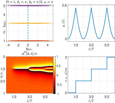
Figure S1: Lines of Fisher zeros, rate function of return probability, geometric phase and dynamical topological invariant of the driven spin chain model. System parameters are chosen as $\Omega=1$, $\delta_{1}=\pi$, $\delta_{2}=\pi/2$, and $\omega=\pi$. The initial state fills the lower Floquet band.

In the first example as shown in Fig. S1, we choose the system parameters to be $\Omega=1$, $\delta_{1}=\pi$, $\delta_{2}=\pi/2$, $\omega=\pi$, and the initial state to be the Floquet modes $\prod_{k>0}|\varphi_{-}(k,t)\rangle$ filling the lower Floquet band. It is directly seen that $|\omega-\delta_{2}|/|\delta_{1}|=1/2<1$. So there will be Floquet DQPTs at critical times $t_{-}=\frac{2n-1}{2}T=2n-1$, and the critical momentum is $k_{c}=\pi/3$. The figure above shows numerical calculation of relevant quantities over three driving periods. We see that each line of Fisher zeros crosses the imaginary time axis at a given critical time. At each of the critical time, the rate function of return probability $g_{-}(t)$ behaves non-analytically as a function of $t$, characterized by a kink structure around each $t_{c}$ and repeating at $t_{c}+nT$ for any $n\in\mathbb{Z}$. Similarly, the number of $2\pi$-jumps in the pattern of geometric phase $\phi_{-}^{{\rm geo}}(k,t)$ versus $k$ increases by $1$ each time when the dynamics passes through a critical time. This is clearly reflected in the behavior of winding number $\nu_{-}(t)$ in time.

In the second example as shown in Fig. S2, we choose the system parameters to be $\Omega=1$, $\delta_{1}=\pi/5$, $\delta_{2}=\pi/2$, $\omega=\pi$, and the initial state still to be the Floquet modes $\prod_{k>0}|\varphi_{-}(k,t)\rangle$ filling the lower Floquet band. This time we have $|\omega-\delta_{2}|/|\delta_{1}|=5/2>1$. So the condition (S49) is not satisfied and there will be no Floquet DQPTs. The numerical calculations of Fisher zeros, rate function of return probability, geometric phase and winding number in three driving periods as presented in Fig. S2 clearly justify this finding.

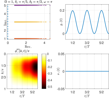
Figure S2: Lines of Fisher zeros, rate function of return probability, geometric phase and dynamical topological invariant of the driven spin chain model. System parameters are chosen as $\Omega=1$, $\delta_{1}=\pi/5$, $\delta_{2}=\pi/2$, and $\omega=\pi$. The initial state fills the lower Floquet band.

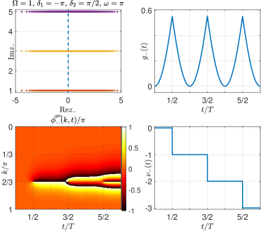
Figure S3: Lines of Fisher zeros, rate function of return probability, geometric phase and dynamical topological invariant of the driven spin chain model. System parameters are chosen as $\Omega=1$, $\delta_{1}=-\pi$, $\delta_{2}=\pi/2$, and $\omega=\pi$. The initial state fills the lower Floquet band.

As a final example shown in Fig. S3, we choose the system parameters to be $\Omega=1$, $\delta_{1}=-\pi$, $\delta_{2}=\pi/2$, $\omega=\pi$, and the initial state to be the Floquet modes $\prod_{k>0}|\varphi_{-}(k,t)\rangle$ filling the lower Floquet band. It is seen that $|\omega-\delta_{2}|/|\delta_{1}|=1/2<1$. So there will be Floquet DQPTs at critical times $t_{-}=\frac{2n-1}{2}T=2n-1$, and the critical momentum is $k_{c}=\frac{2\pi}{3}$. The figure above shows numerical calculation of relevant quantities over three driving periods. We see that each line of Fisher zeros crosses the imaginary time axis at a given critical time. At each of the critical time, the rate function of return probability $g_{-}(t)$ behaves non-analytically as a function of $t$, characterized by a kink structure around each $t_{c}$ and repeating at $t_{c}+nT$ for any $n\in\mathbb{Z}$. Similarly, the number of $2\pi$-jumps in the pattern of geometric phase $\phi_{-}^{{\rm geo}}(k,t)$ versus $k$ increases by $1$ each time when the dynamics passes through a critical time. This is clearly reflected in the behavior of winding number $\nu_{-}(t)$ in time.

II II. Experiment

II.1 A. Experimental setup

The experiment is performed on an NV center in a {100}-face bulk diamond synthesized by chemical vapor deposition (CVD). The nitrogen impurity is less than 5 ppb and the abundance of ¹³C is at the natural level of about 1.1%. The dephasing time of the NV electron spin is 1.7 $\mu$s. The NV center is optically addressed by a home-built confocal microscope. Green laser is used for optical excitation. The laser beam is released and cut off by an acousto-optic modulator (power leakage ratio $\sim 1/1000$). To reduce the laser leakage further, the beam passes twice through the acousto-optic modulator. The laser is focused into the diamond by an oil objective (60*O, NA 1.42). The phonon sideband fluorescence with the wavelength between 650 and 800 nm is collected by the same oil objective and finally detected by an avalanche photodiode with a counter card. A solid immersion lens etched on the diamond by focused ion beam enhances the fluorescence counting rate up to 400 thousand counts per second. The microwaves are generated by an arbitrary waveform generator (AWG) and then strengthened by a power amplifier. Finally, the microwaves are radiated to the NV center from a coplanar waveguide. The magnetic field is supplied by a permanent magnet mounted on a translation stage.

II.2 B. Calibration

The transverse component of the rotating field is $\omega\sin k$. In order to feed the microwaves with proper amplitude to the NV center, we calibrate the Rabi frequency as a function of the AWG’s output amplitude. The calibration is done by performing conventional Rabi oscillation experiments with various output amplitudes. We fit the experimental data of Rabi oscillation associated with each output amplitude $V$ to extract the corresponding Rabi frequency $\omega_{\rm R}$, and then fit the Rabi frequency using $\omega_{\rm R}=a\exp(-V^{2}/b^{2})V$ with $a$ and $b$ being the coefficients to be determined. The relation between the Rabi frequency and the AWG’s output amplitude is thus obtained. Such calibration is carried out hourly to guard against the drift of experimental conditions.

II.3 C. Pulse sequence

After the qubit is polarized to the state $\left|{{\psi_{0}}}\right\rangle={(1,0)^{\rm{T}}}$ by a green laser pulse, a resonant microwave pulse is applied to prepare the initial state. In the laboratory frame, the Hamiltonian of the qubit irradiated by the pulse is

$$H_{{\rm{ini}}}^{{\rm{lab}}}=\frac{\omega_{0}}{2}\sigma_{z}+\omega_{1}\cos({\omega_{0}}t+\varphi_{\rm{ini}})\sigma_{x}.$$ (S66)

where the first term on the right-hand side is the static component of the Hamiltonian with $\omega_{0}$ being the resonant frequency, and the second term accounts for the effect of the microwaves with $\omega_{1}$, $\varphi_{\rm{ini}}$, and $t$ being the Rabi frequency, the initial phase, and the time starting from zero, respectively. The initial phase $\varphi_{\rm{ini}}$ is set as $-\pi/2$ in this experiment. In the rotating frame that rotates around the $z$ axis with the angular frequency $\omega_{0}$, or to put it another way, under the rotating transformation characterized by the rotation operator $R_{\rm{ini}}={e^{-i{\omega_{0}}t{\sigma_{z}}/2}}$, the Hamiltonian in Eq. (S66) is transformed to

$$H_{{\rm{ini}}}^{{\rm{rot}}}={R_{\rm{ini}}^{\dagger}}H_{{\rm{ini}}}^{{\rm{lab}}}R_{\rm{ini}}-i{R_{\rm{ini}}^{\dagger}}\frac{d}{{dt}}R_{\rm{ini}}=\frac{\omega_{1}}{2}(\sigma_{x}\cos\varphi_{\rm{ini}}+\sigma_{y}\sin\varphi_{\rm{ini}}),$$ (S67)

where the second equality relies on the rotating wave approximation. The pulse lasts for $t_{\rm{ini}}=\beta/\omega_{1}$, where $\beta$ is the inclination angle of the initial state, namely,

$$\beta=\pi-\arccos\frac{\delta_{1}\cos k+\delta_{2}-\omega}{{\sqrt{{{(\Omega\sin k)}^{2}}+{{({\delta_{1}}\cos k+{\delta_{2}}-\omega)}^{2}}}}}.$$ (S68)

After the pulse, the state of the qubit in the rotating frame is

$$\left|{\psi_{{\rm{ini}}}^{{\rm{rot}}}}\right\rangle=e^{-iH_{{\rm{ini}}}^{{\rm{rot}}}t_{\rm{ini}}}\left|{{\psi_{0}}}\right\rangle=\left|{\psi{\rm{(}}k,0{\rm{)}}}\right\rangle,$$ (S69)

which is our desired initial state. In the laboratory frame, this state immediately after the pulse is expressed as

$$\left|{\psi_{{\rm{ini}}}^{{\rm{lab}}}}\right\rangle={e^{-i{\omega_{0}}t_{\rm{ini}}{\sigma_{z}}/2}}\left|{\psi_{{\rm{ini}}}^{{\rm{rot}}}}\right\rangle.$$ (S70)

Next, a microwave pulse is applied to build the model Hamiltonian in Eq. (S30). In most cases, this pulse is off-resonant. In the laboratory frame, the Hamiltonian of the qubit irradiated by the pulse is

$$H_{{\rm{evo}}}^{{\rm{lab}}}=\frac{\omega_{0}}{2}\sigma_{z}+\Omega\sin k\cos\left[({\omega_{0}}-{\delta_{1}}\cos k-{\delta_{2}}+\omega)t+\omega_{0}t_{\rm{ini}}\right]\sigma_{x},$$ (S71)

where $t$ is the time starting from zero. In the rotating frame with the rotation operator

$$R_{\rm{evo}}={e^{-i[({\omega_{0}}-{\delta_{1}}\cos k-{\delta_{2}})t+\omega_{0}t_{\rm{ini}}]{\sigma_{z}}/2}},$$ (S72)

the Hamiltonian in Eq. (S71) is transformed to our target Hamiltonian, namely,

$$H_{{\rm{evo}}}^{{\rm{rot}}}={R_{\rm{evo}}^{\dagger}}H_{{\rm{evo}}}^{{\rm{lab}}}R_{\rm{evo}}-i{R_{\rm{evo}}^{\dagger}}\frac{d}{{dt}}R_{\rm{evo}}=\frac{\Omega\sin k}{2}\left[{\cos(\omega t){{\sigma_{x}}}+\sin(\omega t){{\sigma_{y}}}}\right]+\frac{{\delta_{1}}\cos k+{\delta_{2}}}{2}\sigma_{z},$$ (S73)

where the second equality relies on the rotating wave approximation. In this rotating frame, the state in Eq. (S70) is rewritten as

$$R_{\rm{evo}}^{\dagger}(t=0)\left|{\psi_{{\rm{ini}}}^{{\rm{lab}}}}\right\rangle=\left|{\psi_{{\rm{ini}}}^{{\rm{rot}}}}\right\rangle=\left|{\psi{\rm{(}}k,0{\rm{)}}}\right\rangle,$$ (S74)

which has the same form as in the rotating frame defined by $R_{\rm{ini}}$. The pulse lasts for some duration duration $t_{\rm e}$, which is a sampling point in time. Assume that the state of the qubit immediately after the pulse is $\left|{\psi_{{\rm{pump}}}^{{\rm{rot}}}}\right\rangle$ in this rotating frame. In the laboratory frame, the state is expressed as

$$\left|{\psi_{{\rm{evo}}}^{{\rm{lab}}}}\right\rangle={e^{-i[({\omega_{0}}-{\delta_{1}}\cos k-{\delta_{2}})t_{\rm e}+\omega_{0}t_{\rm{ini}}]{\sigma_{z}}/2}}\left|{\psi_{{\rm{evo}}}^{{\rm{rot}}}}\right\rangle.$$ (S75)

Finally, a resonant microwave pulse is applied to assist measurement. In the laboratory frame, the Hamiltonian of the qubit irradiated by the pulse is

$$H_{{\rm{fin}}}^{{\rm{lab}}}=\frac{\omega_{0}}{2}\sigma_{z}+\omega_{1}\cos\left[{{\omega_{0}}t+({\omega_{0}}-{\delta_{1}}\cos k-{\delta_{2}})t_{\rm e}}+\omega_{0}t_{\rm{ini}}+\varphi_{\rm{fin}}\right]\sigma_{x},$$ (S76)

with $\varphi_{\rm{fin}}=\pi/2$. Here $t$ is also the time starting from zero. In the rotating frame with the rotation operator

$$R_{\rm{fin}}={e^{-i[{\omega_{0}}t+({\omega_{0}}-{\delta_{1}}\cos k-{\delta_{2}})t_{\rm e}+\omega_{0}t_{\rm{ini}}]{\sigma_{z}}/2}},$$ (S77)

the Hamiltonian in Eq. (S76) is transformed to

$$H_{{\rm{fin}}}^{{\rm{rot}}}={R_{\rm{fin}}^{\dagger}}H_{{\rm{fin}}}^{{\rm{lab}}}R_{\rm{fin}}-i{R_{\rm{fin}}^{\dagger}}\frac{d}{{dt}}R_{\rm{fin}}=\frac{\omega_{1}}{2}(\sigma_{x}\cos\varphi_{\rm{fin}}+\sigma_{y}\sin\varphi_{\rm{fin}}),$$ (S78)

where the second equality is based on the rotating wave approximation. In this rotating frame, the state in Eq. (S75) is rewritten as

$$R_{\rm{fin}}^{\dagger}(t=0)\left|{\psi_{{\rm{evo}}}^{{\rm{lab}}}}\right\rangle=\left|{\psi_{{\rm{evo}}}^{{\rm{rot}}}}\right\rangle,$$ (S79)

which has the same form as in the rotating frame defined by $R_{\rm{evo}}$. The pulse lasts for $t_{\rm{ini}}=\beta/\omega_{1}$. After the pulse, laser illumination is carried out to measure the probability in $|0\rangle$. The combined effect of the final microwave pulse and its subsequent laser illumination amounts to the measurement of

$$e^{iH_{{\rm{fin}}}^{{\rm{rot}}}t_{\rm{fin}}}|0\rangle\langle 0|e^{-iH_{{\rm{fin}}}^{{\rm{rot}}}t_{\rm{fin}}}=|\psi(k,0)\rangle\langle\psi(k,0)|,$$ (S80)

which yields the return probability $|\langle\psi(k,0)|\psi(k,t)\rangle|^{2}$.

II.4 D. Experimental data analysis

As shown in Fig. 2(c) of the main text, the spin state is read out during the latter laser pulse and there are two counting windows. Such sequence is iterated five hundred thousand times. The total photon count recorded by the first (second) window during these iterations is regarded as signal (reference) and denoted by $s$ ($r$). The raw experimental data is $x=s/r$. To normalize the data, a conventional Rabi oscillation is performed alongside. We fit the raw data of the Rabi oscillation using the function $x=x_{0}+a\cos(\omega_{\rm R}t+\varphi)$, and then normalize the experimental data as $x_{\rm{n}}=(x-x_{0})/(2a)+1/2$. The data thus normalized represent the probability in $|0\rangle$. In the experiment, the sampling points in $t$ are 0, 0.020, 0.040, 0.060, 0.080, 0.094, 0.096, 0.098, 0.100, 0.102, 0.104, 0.106, 0.120, 0.140, 0.160, 0.180, 0.200, 0.220, 0.240, 0.260, 0.280, 0.294, 0.296, 0.298, 0.300, 0.302, 0.304, 0.306, 0.320, 0.340, 0.360, 0.380, 0.400, 0.420, 0.440, 0.460, 0.480, 0.494, 0.496, 0.498, 0.500, 0.502, 0.504, 0.506, 0.520, 0.540, 0.560, 0.580, and 0.600 $\mu$s. In the experiment data illustrated in Figs. 3 and 4(b) of the main text and Figs. S4 and S5(d)-(f) of this supplemental material, the sampling interval in $k$ is $\pi/12$. In the experiment data illustrated in Figs. 4(a) of the main text and Figs. S5(a)-(c), the sampling intervals in $k$ are $\pi/180$. The numerical integration over $k$ is based on the trapezoidal rule.

II.5 E. Method for measuring the geometric phase

The total phase, dynamic phase, and geometric phase, in turn, are

$${\phi_{\alpha}^{{\rm{tot}}}}(k,t)=\arg\left\langle{{\psi_{\alpha}(k,0)}}\mathrel{\left|{\vphantom{{\psi_{\alpha}(k,0)}{\psi_{\alpha}(k,t)}}}\right.\kern-1.2pt}{{\psi_{\alpha}(k,t)}}\right\rangle=-{E_{\alpha}}t-\frac{\omega t}{2}+\arg\left\langle{{\varphi_{\alpha}(k,0)}}\mathrel{\left|{\vphantom{{\varphi_{\alpha}(k,0)}{\varphi_{\alpha}(k,t)}}}\right.\kern-1.2pt}{{\varphi_{\alpha}(k,t)}}\right\rangle+2\pi n,$$ (S81)

$${\phi_{\alpha}^{{\rm{dyn}}}}(k,t)=-\int_{0}^{t}{ds\left\langle{\psi_{\alpha}(k,s)}\right|H(k,s)\left|{\psi_{\alpha}(k,s)}\right\rangle}=-{E_{\pm}}t-\int_{0}^{t}{ds\frac{\omega}{2}\left\langle{\varphi_{\alpha}(k,s)}\right|{\sigma_{z}}\left|{\varphi_{\alpha}(k,s)}\right\rangle}.$$

$${\phi_{\alpha}^{{\rm{geo}}}}(k,t)={\phi_{{\rm{tot}}}}(k,t)-{\phi_{{\rm{dyn}}}}(k,t)=\arg\langle\varphi_{\alpha}(k,0)|\varphi_{\alpha}(k,t)\rangle+\int_{0}^{t}{ds\frac{\omega}{2}\left\langle{\varphi_{\alpha}(k,s)}\right|{\sigma_{z}}\left|{\varphi_{\alpha}(k,s)}\right\rangle}-\frac{\omega t}{2}+2\pi n,$$

where $n$ is an integer. After measuring

$$\langle\sigma_{x}(k,t)\rangle:=\langle\psi_{\alpha}(k,t)|\sigma_{x}|\psi_{\alpha}(k,t)\rangle=\langle\varphi_{\alpha}(k,t)|\sigma_{x}|\varphi_{\alpha}(k,t)\rangle,$$ (S82)

$$\langle\sigma_{y}(k,t)\rangle:=\langle\psi_{\alpha}(k,t)|\sigma_{y}|\psi_{\alpha}(k,t)\rangle=\langle\varphi_{\alpha}(k,t)|\sigma_{y}|\varphi_{\alpha}(k,t)\rangle,$$

$$\langle\sigma_{z}(k,t)\rangle:=\langle\psi_{\alpha}(k,t)|\sigma_{z}|\psi_{\alpha}(k,t)\rangle=\langle\varphi_{\alpha}(k,t)|\sigma_{z}|\varphi_{\alpha}(k,t)\rangle,$$

the inner product $\langle\varphi_{\alpha}(k,0)|\varphi_{\alpha}(k,t)\rangle$ can be calculated. In our experiment, $\alpha=-$ is adopted and we have

$$\langle\varphi_{-}(k,0)|\varphi_{-}(k,t)\rangle=\sin\frac{\theta}{2}\sqrt{\frac{{1+\cos\vartheta}}{2}}-{e^{i\phi}}\cos\frac{\theta}{2}\sqrt{\frac{{1-\cos\vartheta}}{2}},$$ (S83)

where

$$\theta=\arccos\frac{{{\delta_{1}}\cos k+{\delta_{2}}-\omega}}{{\sqrt{{{({\delta_{1}}\cos k+{\delta_{2}}-\omega)}^{2}}+{{(\Omega\sin k)}^{2}}}}}$$ (S84)

$$\vartheta=\arccos\frac{{\left\langle{{\sigma_{z}}(k,t)}\right\rangle}}{{\sqrt{{{\left\langle{{\sigma_{x}}(k,t)}\right\rangle}^{2}}+{{\left\langle{{\sigma_{y}}(k,t)}\right\rangle}^{2}}+{{\left\langle{{\sigma_{z}}(k,t)}\right\rangle}^{2}}}}}$$

$$\phi=\left\{{\begin{array}[]{*{20}{c}}{\arccos\frac{{\left\langle{{\sigma_{x}}(k,t)}\right\rangle}}{{\sqrt{{{\left\langle{{\sigma_{x}}(k,t)}\right\rangle}^{2}}+{{\left\langle{{\sigma_{y}}(k,t)}\right\rangle}^{2}}}}},~{}~{}~{}{\rm{if}}~{}~{}~{}\left\langle{{\sigma_{y}}(k,t)}\right\rangle\geq 0},\\ {-\arccos\frac{{\left\langle{{\sigma_{x}}(k,t)}\right\rangle}}{{\sqrt{{{\left\langle{{\sigma_{x}}(k,t)}\right\rangle}^{2}}+{{\left\langle{{\sigma_{y}}(k,t)}\right\rangle}^{2}}}}},~{}~{}~{}{\rm{if}}~{}~{}~{}\left\langle{{\sigma_{y}}(k,t)}\right\rangle<0}.\\ \end{array}}\right.$$

The geometric phase can then be acquired according to the last expression in Eq. (S81). In this work, the geometric phase is set between $-\pi$ and $\pi$.

II.6 F. Experimental data

The return probabilities for $\delta_{2}=2\pi\times 5$ MHz, $2\pi\times 2.5$ MHz, $-2\pi\times 2.5$ MHz, and $-2\pi\times 5$ MHz are illustrated in Figs. S4(a)-(d), respectively. The return probabilities for $\delta_{2}=2\pi\times 5$ MHz and $-2\pi\times 5$ MHz are also shown in Figs. 3(a) and 3(b) of the main text.

The geometric phase in Fig. 4(a) and (b) of the main text are experimentally acquired from the expectation values of $\sigma_{x}$, $\sigma_{y}$, and $\sigma_{z}$. These expectation values are illustrated in Fig. S5.

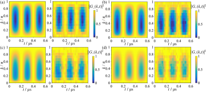
Figure S4: Return probabilities. (a)-(d) Return probabilities for $\delta_{2}=2\pi\times 5$ MHz, $2\pi\times 2.5$ MHz, $-2\pi\times 2.5$ MHz, and $-2\pi\times 5$ MHz, respectively. Calculations based on ideal situations are on the left and experimental data are on the right. All the graphs here share the same color bar.

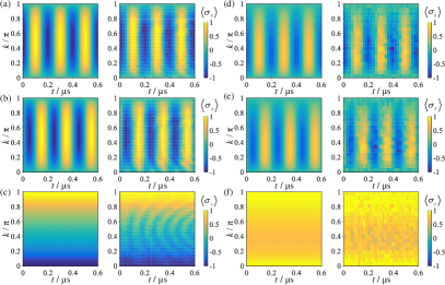
Figure S5: Expectation values of $\sigma_{x}$, $\sigma_{y}$, and $\sigma_{z}$. (a)-(c) Expectation values of $\sigma_{x}$, $\sigma_{y}$, and $\sigma_{z}$ as a function of the synthetic quasimomentum $k$ and the scaled time $\tau$ for $\delta_{2}=5$ MHz. (d)-(f) Expectation values of $\sigma_{x}$, $\sigma_{y}$, and $\sigma_{z}$ as a function of the synthetic quasimomentum $k$ and the scaled time $\tau$ for $\delta_{2}=-5$ MHz. Calculations based on ideal situations are on the left and experimental data are on the right.

References

(1) M. Heyl, A. Polkovnikov, and S. Kehrein, Dynamical
Quantum Phase Transitions in the Transverse-Field Ising Model, Phys.
Rev. Lett. 110, 135704 (2013).
(2) F. Pollmann, S. Mukerjee, A. G. Green,
and J. E. Moore, Dynamics after a sweep through a quantum critical
point, Phys. Rev. E 81, 020101(R) (2010).
(3)
S. Vajna and B. Dóra, Topological classification of dynamical phase transitions, Phys. Rev. B 91, 155127 (2015).
(4) J. C. Budich and M. Heyl, Dynamical topological order
parameters far from equilibrium, Phys. Rev. B 93, 085416
(2016).
(5) C. Yang, L. Li, and S. Chen, Dynamical topological
invariant after a quantum quench, Phys. Rev. B 97, 060304
(2018).
(6) M. Heyl, Dynamical quantum phase transitions:
a review, Rep. Prog. Phys. 81 054001 (2018).
(7) A. A. Zvyagin, Dynamical quantum phase transitions
(Review Article), Low Temp. Phys. 42, 971 (2016).
(8) L. Zhou, Q. Wang, H. Wang, and J. Gong, Dynamical quantum phase transitions in non-Hermitian lattices, Phys. Rev. A 98, 022129 (2018).
(9) P. Jurcevic, H. Shen, P. Hauke, C. Maier, T. Brydges,
C. Hempel, B. P. Lanyon, M. Heyl, R. Blatt, and C. F. Roos, Direct
Observation of Dynamical Quantum Phase Transitions in an Interacting
Many-Body System, Phys. Rev. Lett. 119, 080501 (2017).
(10) J. Zhang, G. Pagano, P. W. Hess, A. Kyprianidis,
P. Becker, H. Kaplan, A. V. Gorshkov, Z.-X. Gong, and C. Monroe, Observation
of a many-body dynamical phase transition with a 53-qubit quantum
simulator, Nature 551, 601-604 (2017).
(11) N. Flschner, D. Vogel, M. Tarnowski,
B. S. Rem, D.-S. Lhmann, M. Heyl, J. C. Budich, L.
Mathey, K. Sengstock, and C. Weitenberg, Observation of dynamical
vortices after quenches in a system with topology, Nat. Phys. 14,
265 (2018).
(12) S. Smale, P. He, B. A. Olsen, K. G. Jackson, H.
Sharum, S. Trotzky, J. Marino, A. Rey, and J. H. Thywissen, Observation
of a Dynamical Phase Transition in the Collective Heisenberg Model,
arXiv:1806.11044 (2018).
(13) X. Guo, C. Yang, Y. Zeng, Y. Peng, H. Li, H. Deng,
Y. Jin, S. Chen, D. Zheng, and H. Fan, Observation of dynamical quantum
phase transition by a superconducting qubit simulation, arXiv:1806.09269
(2018).
(14) T. Tian, Y. Ke, L. Zhang, S. Lin, Z. Shi, P. Huang,
C. Lee, and J. Du, Direct observation of Pancharatnam geometric phase
in a quenched topological system, arXiv:1807.04483 (2018).
(15) K. Wang, X. Qiu, L. Xiao, X. Zhan, Z. Bian, W.
Yi, and P. Xue, Simulating dynamic quantum phase transitions in photonic
quantum walks, arXiv:1806.10871 (2018).
(16) X. Xu, Q. Wang, M. Hey, J. C. Budich, W. Pan,
Z. Chen, M. Jan, K. Sun, J. Xu, Y. Han, C. Li, and G. Guo, Measuring
a Dynamical Topological Order Parameter in Quantum Walks, arXiv:1808.03930
(2018).
(17) S. Sharma, U. Divakaran, A. Polkovnikov, and A. Dutta, Slow quenches in a quantum Ising chain: Dynamical phase transitions and topology, Phys. Rev. B 93, 144306 (2016).
(18) T. Pukarov and D. Schuricht, Time evolution during and after finite-time quantum quenches in the transverse-field Ising chain, SciPost Phys. 1, 003 (2016).
(19) U. Bhattacharya and A. Dutta, Interconnections between equilibrium topology and dynamical quantum phase transitions in a linearly ramped Haldane model, Phys. Rev. B 95, 184307 (2017).
(20)
N. H. Lindner, G. Refael, and V. Galitski, Floquet topological insulator in semiconductor quantum wells, Nature Phys. 7, 490 (2011).
(21) J. Cayssol, B. Dóra, F. Simon, and R. Moessner,
Floquet topological insulators, Phys. Status Solidi RRL, 7, 101-108 (2013).
(22) L. Zhou, H. Wang, D. Y. H. Ho and J. Gong,
Aspects of Floquet Bands and Topological Phase Transitions in a Continuously Driven Superlattice, EPJB 87, 204 (2014).
(23) D. Y. H. Ho and J. Gong, Quantized Adiabatic
Transport in Momentum Space, Phys. Rev. Lett. 109, 010601
(2012).
(24) L. Li, C. H. Lee, and J. Gong, Realistic Floquet
semimetal with exotic topological linkages between arbitrarily many
nodal loops, Phys. Rev. Lett. 121, 036401 (2018).
(25) K. Sacha and J. Zakrzewski, Time crystals: a review,
Rep. Prog. Phys. 81, 016401 (2018).
(26)
N. Y. Yao and C. Nayak, Time crystals in periodically driven systems, Physics Today 71, 9, 40 (2018).
(27) R. W. Bomantara and J. Gong, Simulation of
Non-Abelian braiding in Majorana time crystals, Phys. Rev. Lett. 120,
230405 (2018).
(28) A. Kosior and K. Sacha, Dynamical quantum phase
transitions in discrete time crystals, Phys. Rev. A 97, 053621
(2018).
(29) A. Kosior, A. Syrwid, and K. Sacha, Dynamical quantum
phase transitions in systems with broken continuous time and space
translation symmetries, Phys. Rev. A 98, 023612 (2018).
(30) M. Holthaus, Floquet engineering with quasienergy
bands of periodically driven optical lattices, J. Phys. B: At. Mol.
Opt. Phys. 49, 013001 (2016).
(31) See Sec. I B in the Supplemental Material for a more detailed review of the Floquet theory; Sec. I A and C for details about static and Floquet DQPTs; Sec. I D for details about the driven spin chain model; Sec. I E for details about Floquet DQPTs in the driven spin chain model.
(32) W. Ma, L. Zhou, Q. Zhang, M. Li, C. Cheng, J. Geng,
X. Rong, F. Shi, J. Gong, and J. Du, Experimental Observation of a
Generalized Thouless Pump with a Single Spin, Phys. Rev. Lett. 120,
120501 (2018).
(33) J. K. Asbth and H. Obuse,
Bulk-boundary correspondence for chiral symmetric quantum walks, Phys.
Rev. B 88, 121406(R) (2013).
(34)
M. W. Doherty, N. B. Manson, P. Delaney, F. Jelezko, J. Wrachtrup, and L. C. L. Hollenberg, The nitrogen-vacancy colour centre in diamond, Phys. Rep. 528, 1 (2013).
(35)
R. Schirhagl, K. Chang, M. Loretz, and C. L. Degen, Nitrogen-Vacancy Centers in Diamond: Nanoscale Sensors for Physics and Biology, Annu. Rev. Phys. Chem. 65, 83 (2014).
(36)
S. Prawer and I. Aharonovich, Quantum Information Processing with Diamond (Woodhead Publishing, Cambridge, England, 2014).
(37)
J. Wrachtrup and A. Finkler, Single spin magnetic resonance, J. Magn. Reson. 269, 225 (2016).
(38)
V. Jacques, P. Neumann, J. Beck, M. Markham, D. Twitchen, J. Meijer, F. Kaiser, G. Balasubramanian, F. Jelezko, and J. Wrachtrup, Dynamic Polarization of Single Nuclear Spins by Optical Pumping of Nitrogen-Vacancy Color Centers in Diamond at Room Temperature, Phys. Rev. Lett. 102, 057403 (2009).
(39)
T. van der Sar, Z. H. Wang, M. S. Blok, H. Bernien, T. H. Taminiau, D. M. Toyli, D. A. Lidar, D. D. Awschalom, R. Hanson, and V. V. Dobrovitski, Decoherence-protected quantum gates for a hybrid solid-state spin register, Nature (London) 484, 82 (2012).
(40)
L. Robledo, L. Childress, H. Bernien, B. Hensen, P. F. A. Alkemade, and R. Hanson, High-fidelity projective read-out of a solid-state spin quantum register, Nature (London) 477, 574 (2011).
(41)
X. Rong, J. Geng, F. Shi, Y. Liu, K. Xu, W. Ma, F. Kong, Z. Jiang, Y. Wu, and J. Du, Experimental fault-tolerant universal quantum gates with solid-state spins under ambient conditions, Nat. Commun. 6, 8748 (2015).
(42)
The error bars of the experimental rate functions are not shown here because some bars are extroadanary long.
This is due to the nearly vanishing return probabilities around the critical quasimomenta and critical times.
(43) F. Franchini, An Introduction to Integrable
Techniques for One-Dimensional Quantum Systems, Lecture Notes in
Physics 940 (Springer, Cham., 2017).
(44) P. Coleman, Introduction to Many-Body
Physics (Cambridge, United Kingdom, 2015).
(45) A. Y. Kitaev, Unpaired Majorana fermions in quantum
wires, Phys.-Usp. 44, 131 (2001).
Supplemental Material

References

(1) M. Heyl, A. Polkovnikov, and S. Kehrein, Dynamical
Quantum Phase Transitions in the Transverse-Field Ising Model, Phys.
Rev. Lett. 110, 135704 (2013).
(2) M. Heyl, Dynamical quantum phase transitions:
a review, Rep. Prog. Phys. 81 054001 (2018).
(3) P. Jurcevic, H. Shen, P. Hauke, C. Maier, T. Brydges,
C. Hempel, B. P. Lanyon, M. Heyl, R. Blatt, and C. F. Roos, Direct
Observation of Dynamical Quantum Phase Transitions in an Interacting
Many-Body System, Phys. Rev. Lett. 119, 080501 (2017).
(4) M. Holthaus, Floquet
engineering with quasienergy bands of periodically driven optical
lattices, J. Phys. B: At. Mol. Opt. Phys. 49, 013001 (2016).
(5) F. Franchini, An
Introduction to Integrable Techniques for One-Dimensional Quantum
Systems, Lecture Notes in Physics 940 (Springer, Cham.,
2017).
(6) W. Ma, L. Zhou, Q. Zhang, M. Li, C. Cheng, J. Geng,
X. Rong, F. Shi, J. Gong, and J. Du, Experimental Observation of a
Generalized Thouless Pump with a Single Spin, Phys. Rev. Lett. 120,
120501 (2018).
(7) J. K. Asbth and H. Obuse,
Bulk-boundary correspondence for chiral symmetric quantum walks, Phys.
Rev. B 88, 121406(R) (2013).
(8) J. Samuel and R. Bhandari, General Setting for
Berry’s Phase, Phys. Rev. Lett. 60, 2339 (1988).
(9) For situations in non-Floquet systems, see
J. C. Budich and M. Heyl, Dynamical topological order parameters far
from equilibrium, Phys. Rev. B 93, 085416 (2016).