Computing Optimal Assignments in Linear Time for Approximate Graph Matching

Abstract

Finding an optimal assignment between two sets of objects is a fundamental problem arising in many applications, including the matching of ‘bag-of-words’ representations in natural language processing and computer vision. Solving the assignment problem typically requires cubic time and its pairwise computation is expensive on large datasets. In this paper, we develop an algorithm which can find an optimal assignment in linear time when the cost function between objects is represented by a tree distance. We employ the method to approximate the edit distance between two graphs by matching their vertices in linear time. To this end, we propose two tree distances, the first of which reflects discrete and structural differences between vertices, and the second of which can be used to compare continuous labels. We verify the effectiveness and efficiency of our methods using synthetic and real-world datasets.

I Introduction

Vast amounts of data are now available for machine learning, including text documents, images, graphs and many more. Learning from such data typically involves computing a similarity or distance function between the data objects. Since many of these datasets are large, the efficiency of the comparison methods is critical. This is particularly challenging since taking the structure adequately into account often is a hard problem. For example, no polynomial-time algorithms are known even for the basic task to decide whether two graphs have the same structure [1]. Therefore, the pragmatic approach of describing such data with a ‘bag-of-words’ or ‘bag-of-features’ is commonly used. In this representation, a series of objects are identified in the data and each object is described by a label or feature. The labels are placed in a bag where the order in which they appear does not matter.

In the most basic form, such bags can be represented by histograms or feature vectors, two of which are compared by counting the number of co-occurrences of a label in the bags. This is a common approach not only for images and text, but also for graph comparison, where a number of graph kernels have been proposed which use different substructures as elements of the bag [2, 3]. In the more general case, two bags of features are compared by summing over all pairs of features weighted by a similarity function between the features. However, in both cases, the method is not ideal, since each feature corresponds to a specific element in the data object, and so can correspond to no more than one element in a second data object. The co-occurrence counting method allows each feature to match to multiple features in the other dataset.

A different approach is to explicitly find the best correspondence between the features of two bags. This can be achieved by solving the (linear) assignment problem in $O(n^{3})$ time using Hungarian-type algorithms [4]. When we assume weights to be integers within the range of $[0,N]$, scaling algorithm become applicable such as [5], which requires $O(n^{2.5}\log N)$ time. Several authors studied a geometric version of the problem, where the objects are points in $\mathbb{R}^{d}$ and the total distance is to be minimised. No subquadratic exact algorithm for this task is known, but efficient approximation algorithms exist [6]. This is also the case for various other problem variants, see [7] and references therein. These algorithms are typically involved and focus on theoretical guarantees. For practical applications often standard algorithms with cubic running time, simple greedy strategies or methods specifically designed for one task are used.

We briefly summarise the use of assignment methods for comparing structured data in machine learning with a focus on graphs. While most kernels for such data are based on co-occurrence counting, there has been growing interest in deriving kernels from optimal assignments in recent years. The pyramid match kernel was proposed to approximate correspondences between bags of features in $\mathbb{R}^{d}$ by employing a space-partitioning tree structure and counting how often points fall into the same bin [8]. For graphs, the optimal assignment kernel was proposed, which establishes a correspondence between the vertices of two graphs using the Hungarian algorithm [9]. However, it was soon realised that this approach does not lead to valid kernels in the general case [2]. Therefore, Johansson and Dubhashi [10] derived kernels from optimal assignments by first sampling a fixed set of so-called landmarks and representing graphs by their optimal assignment similarities to landmarks. Kriege et al. [11] demonstrated that a specific choice of a weight function (derived from a hierarchy) does in fact generate a valid kernel for the optimal assignment method and allows computation in linear time. The approach is not designed to actually construct the assignment.

The term graph matching refers to a diverse set of techniques which typically establish correspondences between the vertices (and edges) of two graphs [12, 13]. This task is closely related to the classical $\mathsf{NP}$-hard maximum common subgraph problem, which asks for the largest graph that is contained as subgraph in two given graphs [1]. Exact algorithms for this problem haven been studied extensively, e.g., for applications in cheminformatics [14], where small molecular graphs with about 20 vertices are compared. The term network alignment is commonly used in bioinformatics, where large networks with thousands of vertices are compared such as protein-protein interaction networks. Methods applicable to such graphs typically cannot guarantee that an optimal solution is found and often solve the assignment problem as a subroutine, e.g., [15, 16]. In the following we will focus on the graph edit distance, which is one of the most widely accepted approaches to graph matching with applications ranging from cheminformatics to computer vision [17]. It is defined as the minimum cost of edit operations required to transform one graph into another graph. The concept has been proposed for pattern recognition tasks more than 30 years ago [18]. However, its computation is $\mathsf{NP}$-hard, since it generalises the maximum common subgraph problem [19]. The graph edit distance is closely related to the notoriously hard quadratic assignment problem [20]. Recently several elaborated exact algorithms for computing the graph edit distance have been proposed [21, 22, 23]. Binary linear programming formulations in combination with highly-optimised general purpose solvers are among the most efficient approaches, but are still limited to small graphs [22]. Even a restricted special case of the graph edit distance is $\mathsf{APX}$-hard [24], i.e., there is a constant $c>1$, such that no polynomial-time algorithm can approximate it within the factor $c$, unless $\mathsf{P}$=$\mathsf{NP}$. However, heuristics based on the assignment problem turned out to be effective tools [25] and are widely used in practice [17]. The original approach requires cubic running time, which is still not feasible for large graphs. Therefore, it has been proposed to use non-exact algorithms for solving the assignment problem. Simple greedy algorithms reduce the running time to $O(n^{2})$ [26, 27]. For large graphs the quadratic running time is still problematic in practice. Moreover, many applications require a large number of distance computations, e.g., for solving classification tasks or performing similarity search in graph databases [28].

Our contribution

We develop a practical algorithm, which solves the assignment problem exactly in linear time when the cost function is a tree metric. A tree metric can be represented compactly by a weighted tree of linear size, which we use for constructing an optimal assignment. We show how to embed sets of objects in an $\ell_{1}$ space preserving the optimal assignment costs. In order to demonstrate that our approach is—despite its simplicity—suitable for challenging real-world problems, we use it for approximating the graph edit distance. To this end, we propose two techniques for generating trees representing cost functions: (i) based on Weisfeiler-Lehman refinement to quantify discrete and structural differences, (ii) based on hierarchical clustering for continuous vertex attributes. We show experimentally that our linear time assignment algorithm scales to large graphs and datasets. Our approach outperforms both exact and approximate methods for computing the graph edit distance in terms of running time and provides state-of-the-art classification accuracy. For some datasets with discrete labels our method even beats these approaches in terms of accuracy.

II Fundamentals

We summarise basic concepts and results on graphs, tree distances, the assignment problem and the graph edit distance.

II-A Graph theory

An undirected graph $G=(V,E)$ consists of a finite set $V(G)=V$ of vertices and a finite set $E(G)=E$ of edges, where each edge connects two distinct vertices. We denote an edge connecting a vertex $u$ and a vertex $v$ by $uv$ or $vu$, where both refers to the same edge. Two vertices $u$ and $v$ are said to be adjacent if $uv\in E$ and referred to as endpoints of the edge $uv$. The vertices adjacent to a vertex $v$ in $G$ are denoted by $N_{G}(v)=\{u\in V(G)\mid uv\in E(G)\}$ and referred to as neighbours of $v$. A path of length $n$ is a sequence of vertices $(v_{0},\dots,v_{n})$ such that $v_{i}v_{i+1}\in E$ for $0\leq i<n$. A weighted graph is a graph $G$ endowed with a weight function $w:E(G)\to\mathbb{R}$. The length of a path in a weighted graph refers to the sum of weights of the edges contained in the path. A graph $G^{\prime}=(V^{\prime},E^{\prime})$ is a subgraph of a graph $G=(V,E)$, written $G^{\prime}\subseteq G$, if $V^{\prime}\subseteq V$ and $E^{\prime}\subseteq E$. Let $V^{\prime}\subseteq V$, then $G^{\prime}=(V^{\prime},E^{\prime})$ with $E^{\prime}=\{uv\in E\mid u,v\in V^{\prime}\}$ is said to be the subgraph induced by $V^{\prime}$ in $G$ and is denoted by $G[V^{\prime}]$. An isomorphism between two graphs $G$ and $H$ is a bijection $\psi:V(G)\to V(H)$ such that $uv\in E(G)\Leftrightarrow\psi(u)\psi(v)\in E(H)$ for all $u,v\in V(G)$. Two graphs $G$ and $H$ are said to be isomorphic if an isomorphism between $G$ and $H$ exists. An automorphism of a graph $G$ is an isomorphism $\psi:V(G)\to V(G)$.

II-B Tree metrics and ultrametrics

A dissimilarity function $d:\mathcal{X}\times\mathcal{X}$ is a metric on $\mathcal{X}$, if it is (i) non-negative, (ii) symmetric, (iii) zero iff two objects are equal and (iv) satisfies the triangle inequality. A metric $d$ on $\mathcal{X}$ is an ultrametric if it satisfies the strong triangle inequality $d(x,y)\leq\max\{d(x,z),d(z,y)\}$ for all $x,y,z\in\mathcal{X}$. A metric $d$ on $\mathcal{X}$ is a tree metric if $d(x,y)+d(v,w)\leq\max\{d(x,v)+d(y,w),d(x,w)+d(y,v)\}$ for all $v,w,x,y\in\mathcal{X}$.

These restricted classes of distances can equivalently be defined in terms of path lengths in weighted trees, which has been investigated in detail, e.g., in phylogentics [29]. A weighted tree $T$ with positive real-valued edge weights $w:E(T)\to\mathbb{R}_{>0}$ represents the distance $d:V(T)\times V(T)\to\mathbb{R}_{\geq 0}$ defined as $d_{(T,w)}(u,v)=\sum_{e\in P(u,v)}w(e)$, where $P(u,v)$ denotes the unique path from $u$ to $v$, for all $u,v\in V(T)$. For every ultrametric $d$ on $\mathcal{X}$ there is a rooted tree $T$ with leaves $\mathcal{X}$ and positive real-valued edge weights, such that (i) $d$is the path length between leaves in $T$, (ii) all paths from any leaf to the root have equal length. For every tree metric $d$ on $\mathcal{X}$ there is a tree $T$ with $\mathcal{X}\subseteq V(T)$ and positive real-valued edge weights, such that $d$ corresponds to the path lengths in $T$. Note that an ultrametric always is a tree metric. For the clarity of notation we distinguish between the elements of $\mathcal{X}$ and the nodes of a tree $T$ by introducing an injective map $\varphi:\mathcal{X}\to V(T)$. We will refer to both a label $u\in\mathcal{X}$ and the associated node by the same letter, with the meaning clear from the context. We consider the distance $d:\mathcal{X}\times\mathcal{X}\to\mathbb{R}_{\geq 0}$ defined as $d(x,y)=d_{(T,w)}(\varphi(x),\varphi(y))$.

II-C The assignment problem

The assignment problem is a well-studied classical combinatorial problem [4]. Given a triple $(A,B,c)$, where $A$ and $B$ are sets of distinct objects with $|A|=|B|=n$ and $c:A\times B\to\mathbb{R}$ a cost function, the problem asks for a one-to-one correspondence $M$ between $A$ and $B$ with minimum costs. The cost of $M$ is $c(M)=\sum_{(a,b)\in M}c(a,b)$. Assuming an arbitrary, but fixed ordering of the elements of $A$ and $B$, an assignment instance can also be given by a cost matrix $\mathbf{C}\in\mathbb{R}^{n\times n}$, where $c_{i,j}=c(a_{i},b_{j})$ and $a_{i}$ is the $i$th element of $A$ and $b_{j}$ is the $j$th element of $B$. Note that in this case the input $\mathbf{C}$ is of size $\Theta(n^{2})$, where otherwise the input size depends on the representation of the cost function $c$. The assignment problem is equivalent to finding a minimum weight perfect matching in a complete bipartite graph on the two sets $A$ and $B$ with edge weights according to $c$. Unless $\mathbf{C}$ is sparse or contains only integral values from a bounded interval, the best known algorithms require cubic time, which is achieved by the well-known Hungarian method.

Here we consider the assignment problem for two sets of objects where the objects are labelled by elements of $\mathcal{X}$. There exists a labelling $\ell:A\cup B\to\mathcal{X}$ associating each object $a\in A\cup B$ with a label $\ell(a)\in\mathcal{X}$. Furthermore, we may associate objects with tree nodes using the map $\varrho=\varphi\cdot\ell$. We then have $c(a,b)=d(\ell(a),\ell(b))=d_{(T,w)}(\varrho(a),\varrho(b))$. We denote by $D^{c}_{\mathrm{OA}}(A,B)$ the cost of an optimal assignment between $A$ and $B$, and the assignment problem as the quadruple $(A,B,T,\varrho)$.

II-D The graph edit distance

The graph edit distance measures the minimum cost required to transform a graph into another graph by adding, deleting and substituting vertices and edges. Each edit operation $o$ is assigned a cost $c(o)$, which may depend on the attributes associated with the affected vertices and edges. A sequence of $k$ edit operations $(o_{1},\dots,o_{k})$ that transforms a graph $G$ into another graph $H$ is called an edit path from $G$ to $H$. We denote the set of all possible edit paths from $G$ to $H$ by $\Upsilon(G,H)$. Let $G$ and $H$ be attributed graphs, the graph edit distance from $G$ to $H$ is defined by

$$d(G,H)=\min\left\{\sum_{i=1}^{k}\,c(o_{i})\mathrel{}\middle|\mathrel{}(o_{1},\dots,o_{k})\in\Upsilon(G,H)\right\}\,.$$

In order to obtain a meaningful measure of dissimilarity for graphs, a cost function must be tailored to the particular attributes that are present in the considered graphs.

Approximating the graph edit distance by assignments

Computing the graph edit distance is an $\mathsf{NP}$-hard problem and solving practical instances by exact approaches is often not feasible. Therefore, Riesen and Bunke [25] proposed to derive a suboptimal edit path between graphs from an optimal assignment of their vertices, where the assignment costs also encode the local edge structure. For two graphs $G$ and $H$ with vertices $U=\{u_{1},\dots,u_{n}\}$ and $V=\{v_{1},\dots,v_{m}\}$, an assignment cost matrix $\mathbf{C}$ is created according to

$$\mathbf{C}=\begin{bmatrix}[cccc|cccc]c_{1,1}&c_{1,2}&\cdots&c_{1,m}&c_{1,\epsilon}&\infty&\cdots&\infty\\ c_{2,1}&c_{2,2}&\cdots&c_{2,m}&\infty&c_{2,\epsilon}&\ddots&\vdots\\ \vdots&\vdots&\ddots&\vdots&\vdots&\ddots&\ddots&\infty\\ c_{n,1}&c_{n,2}&\cdots&c_{n,m}&\infty&\cdots&\infty&c_{n,\epsilon}\\ \cline{1-8}\cr c_{\epsilon,1}&\infty&\cdots&\infty&0&0&\cdots&0\\ \infty&c_{\epsilon,2}&\ddots&\vdots&0&0&\ddots&\vdots\\ \vdots&\ddots&\ddots&\infty&\vdots&\ddots&\ddots&0\\ \infty&\cdots&\infty&c_{\epsilon,m}&0&\cdots&0&0\\ \end{bmatrix},$$ (1)

where the entries are estimations of the cost for substituting, deleting and inserting vertices in $G$. In more detail, the entry $c_{i,\epsilon}$ is the cost for deleting $u_{i}$ increased by the costs for deleting the edges incident to $u_{i}$. The entry $c_{\epsilon,j}$ is the cost for inserting $v_{j}$ and all edges incident to $v_{j}$. Finally $c_{i,j}$ is the cost made up of the cost for substituting the vertex $u_{i}$ by $v_{j}$ and the cost of an optimal assignment between the incident edges w.r.t. the edge substitution, deletion and insertion costs. An optimal assignment for $\mathbf{C}$ allows to derive an edit path between $G$ and $H$. Its cost is not necessarily minimum possible, but Riesen and Bunke [25] show experimentally that this procedure leads to a sufficiently good approximation of the graph edit distance for many real-world problems.

The costs derived by Riesen and Bunke [25] are directly related to edit costs of various operations on the graph, but unfortunately these costs are not suitable for our optimal assignment strategy, which must utilise a tree metric. For this reason, we use a different set of costs, described in Section IV. The optimal assignment is recovered using the method described in the next section. This assignment then induces an edit path which is used to compute a good approximation to the edit distance.

III Optimal assignments under a tree metric

We consider the assignment problem under the assumption that the costs are derived from a tree metric and propose an efficient algorithm for constructing a solution. For a dataset of sets of objects we obtain a distance-preserving embedding of the pairwise optimal assignment costs into an $\ell_{1}$ space.

III-A Structural results

(a) Tree representing a metric

	$\overleftarrow{su}$	$\overleftarrow{tu}$	$\overleftarrow{uv}$	$\overleftarrow{vw}$	$\overleftarrow{vx}$	$\overrightarrow{su}$	$\overrightarrow{tu}$	$\overrightarrow{uv}$	$\overrightarrow{vw}$	$\overrightarrow{vx}$
$A$	0	2	2	2	5	5	3	3	3	0
$B$	2	1	3	4	4	3	4	2	1	1

(a) Partition size w.r.t. oriented edges

Figure 1: A tree representing a metric and the objects of an assignment instance associated to its nodes. In this instance $A=\{a_{1},a_{2},a_{3},a_{4},a_{5}\}$ and these objects are labelled $(t,t,w,w,w)$. Similarly the five objects in $B$ are labelled $(s,s,t,w,x)$. The objects are associated to tree nodes by the map $\varrho$, and denotes the elements of the set $A$ and of $B$, respectively.

Let $(A,B,T,\varrho)$ be an assignment instance as described in Section II-C. We associate the objects of $A$ and $B$ with the nodes of the tree $T$ according to the map $\varrho$, cf. Figure 1(a). An assignment $M$ between the objects of $A$ and $B$ is associated with a collection of paths $\mathcal{P}$ in $T$, such that there is a bijection between pairs $(a,b)\in M$ and paths $(\varrho(a),\dots,\varrho(b))\in\mathcal{P}$. In particular, the cost of the assignment equals the sum of path lengths, i.e.,

$$c(M)=\sum_{P\in\mathcal{P}}\sum_{e\in P}w(e).$$ (2)

We do not construct the set $\mathcal{P}$ explicitly, but use this notion to develop efficient methods and prove their correctness. Using Eq. (2), we can attribute the total costs of an optimal assignment to the individual edges by counting how often they occur on paths. Deleting an arbitrary edge $uv$ yields two connected components, one containing the node $u$ and the other containing $v$. Let $A_{\overleftarrow{uv}}$ and $A_{\overrightarrow{uv}}$ denote the number of objects in $A$ associated by $\varrho$ with nodes in the connected component containing $u$ and $v$, respectively, cf. Figure I(a).

Lemma 1.

Let $\mathcal{P}$ be the collection of paths associated with an optimal assignment between $A$ and $B$ under a cost function represented by the weighted tree $T$. Each edge $uv$ in $T$ appears $|A_{\overleftarrow{uv}}-B_{\overleftarrow{uv}}|=|A_{\overrightarrow{uv}}-B_{\overrightarrow{uv}}|$ times in a path in $\mathcal{P}$.

Proof.

Splitting $T$ at an edge defines a bipartition of $A$ and $B$. Since $|A|=|B|$ holds, it follows that $|A_{\overleftarrow{uv}}-B_{\overleftarrow{uv}}|=|A_{\overrightarrow{uv}}-B_{\overrightarrow{uv}}|$ for every edge $uv$. When $uv$ appears in $|A_{\overleftarrow{uv}}-B_{\overleftarrow{uv}}|$ assignment paths, the maximum number of assignments is made within each subset, with all of the smaller of $A$ and $B$ assigned within the subset. We may assign at most $\min\{A_{\overleftarrow{uv}},B_{\overleftarrow{uv}}\}$ objects within the connected component containing $u$, and at least the remaining $|A_{\overleftarrow{uv}}-B_{\overleftarrow{uv}}|$ objects must be assigned to objects in the connected component containing $v$. Therefore, $uv$ appears at least this number of times in paths in $\mathcal{P}$.

It remains to be shown that the assignment cannot be optimal when the edge $uv$ is contained in more paths. Assume $\mathcal{P}^{\prime}$ corresponds to an optimal solution and contains the edge $uv$ more than $|A_{\overleftarrow{uv}}-B_{\overleftarrow{uv}}|$ times. Then, there are $a_{1}\in A$ and $b_{2}\in B$ in the connected component containing $u$, which are both assigned across the partition to elements $b_{1}\in B$ and $a_{2}\in A$, respectively, in the component containing $v$. The corresponding assignment paths $P_{1}=(a_{1},\dots,u,v,\dots,b_{1})$ and $P_{2}=(b_{2},\dots,u,v,\dots,a_{2})$ are contained in $\mathcal{P}^{\prime}$. Consider the paths $P^{\prime}_{1}=(a_{1},\dots,u,\dots,b_{2})$ and $P^{\prime}_{2}=(a_{2},\dots,v,\dots,b_{1})$, which both do not contain $uv$. The collection of paths $\mathcal{P}^{\prime\prime}=\mathcal{P}^{\prime}\cup\{P^{\prime}_{1},P^{\prime}_{2}\}\setminus\{P_{1},P_{2}\}$ also defines an assignment, where the edges are contained in the same number of paths with exception of the edge $uv$, which appears in two paths less. Since $w(uv)>0$, the associated solution has cost $c(\mathcal{P}^{\prime\prime})=c(\mathcal{P}^{\prime})-2w(uv)$ and hence $\mathcal{P}^{\prime}$ cannot correspond to an optimal solution, contradicting the assumption. ∎

This result allows us to compute the optimal assignment cost as a weighted sum over the edges in the tree representing the cost metric.

Theorem 2.

Let $(A,B,T,\varrho)$ be an assignment instance with tree edge weights $w$. The cost of an optimal assignment is

$$D^{c}_{\mathrm{OA}}(A,B)=\sum_{uv\in E(T)}|A_{\overleftarrow{uv}}-B_{\overleftarrow{uv}}|\cdot w(uv).$$

Proof.

Directly follows from Eq. (2) and Lemma 1. ∎

III-B Constructing an optimal assignment

In order to compute an optimal assignment, and not just its cost, we again associate the objects of $A$ and $B$ with the nodes of the tree $T$. Then we pick an arbitrary leaf $v$ and match the maximum possible number of elements between the subsets of $A$ and $B$ associated with $v$. The remaining objects are passed to its neighbour and the considered leaf is deleted. Iterating the approach until the tree is eventually empty, yields an assignment between all objects of $A$ and $B$. Algorithm 1 implements this approach.

Input: Assignment instance $(A,B,T,\varrho)$.

Data: Subsets $A_{v}\subseteq A$ and $B_{v}\subseteq B$ for each vertex $v$ of $T$, partial assignment $M$.

Output: An optimal assignment $M$.

1

2forall $a\in A$ do  $A_{\varrho(a)}\leftarrow A_{\varrho(a)}\cup\{a\}$

3  $\triangleright$ Initialisation forall $b\in B$ do  $B_{\varrho(b)}\leftarrow B_{\varrho(b)}\cup\{b\}$

4

5$M\leftarrow\emptyset$

6 while $V(T)\neq\emptyset$ do

7       $v\leftarrow$ arbitrary vertex in $T$ with degree $1$

8       $M\leftarrow M\cup\textnormal{{PairElements}}(A_{v},B_{v})$

       $n\leftarrow\textnormal{{Neighbour}}(v)$

        $\triangleright$ Get distinct neighbour

       $A_{n}\leftarrow A_{n}\cup A_{v}$

        $\triangleright$ Pass unmatched objects

9       $B_{n}\leftarrow B_{n}\cup B_{v}$

       $T\leftarrow T\setminus v$

        $\triangleright$ Remove the node $v$ from $T$

10      

Procedure PairElements($A_{v},B_{v}$)

11       $X\leftarrow\emptyset$

12       while $A_{v}\neq\emptyset$ and $B_{v}\neq\emptyset$ do

13             $a\leftarrow\textnormal{{PickElement}}(A_{v})$;  $A_{v}\leftarrow A_{v}\setminus\{a\}$

14             $b\leftarrow\textnormal{{PickElement}}(B_{v})$;  $B_{v}\leftarrow B_{v}\setminus\{b\}$

15             $X\leftarrow X\cup\{(a,b)\}$

16            

17      return $X$

18      

Algorithm 1 Optimal assignment from a cost tree.

Theorem 3.

Algorithm 1 computes an optimal assignment in time $O(n+t)$, where $n=|A|=|B|$ is the input size and $t=|V(T)|$ the size of the tree $T$.

Proof.

Since $|A|=|B|$ and every object of $A$ is associated with exactly one object of $B$, the algorithm constructs an assignment. The cost of the assignment corresponds to the number of objects that are passed to neighbours along the weighted edges in lines 1 and 1. Whenever a node $v$ is processed in the while-loop, it has exactly one remaining neighbour $n$. Since $v$ is deleted after the end of the iteration, objects are passed along the edge $nv$ only in this iteration. After calling the procedure PairElements in line 1 either$A_{v}$ or $B_{v}$ or both are empty. Since all objects in the connected component of $T\setminus nv$ that contains $v$ must have been passed to $v$ in previous iterations, exactly $|A_{\overleftarrow{nv}}-B_{\overleftarrow{nv}}|$ objects are passed to $n$. This is the number of occurrences of $nv$ in every optimal solution according to Lemma 1. Therefore, $M$ is an optimal assignment.

The total running time over all iterations for the procedure PairElements is $O(n)$, the size of the assignment. All the other individual operations within the while-loop can be implemented in constant time when using linked lists to store and pass the objects. Therefore the while-loop and the entire algorithm run in $O(n+t)$ total time. ∎

Every optimal assignment can be obtained by Algorithm 1 depending on the order in which the objects are retrieved by PickElement in line 1 and 1.

III-C Improving the running time

We consider the setting, where the map $\varrho$ and the weighted tree $(T,w)$ encoding the cost metric $c$ are fixed and the distance $D^{c}_{\mathrm{OA}}$ should be computed for a large number of pairs. The individual assignment instances possibly only populate a small fraction of the nodes of $T$ and only a small subtree may be relevant for Algorithm 1. We show that this subtree can be identified efficiently.

Given a tree $T$ and a set $N\subseteq V(T)$, let $T_{N}$ denote the minimal subtree of $T$ with $N\subseteq V(T_{N})$.

Lemma 4.

Given a tree $T$ and a set $N\subseteq V(T)$, the subtree $T_{N}$ can be computed in time $O(|V(T_{N})|)$ after a preprocessing step of time $O(|V(T)|)$.

Proof.

In the preprocessing step we pick an arbitrary node of $T$ as root and compute the depth of every vertex w.r.t. the root using breadth-first search. Let $d_{\min}=\min\{\operatorname{depth}(v)\mid v\in N\}$. For every node $v\in N$, we (i) add $v$ to the result set $R$, and (ii) if the parent $p$ of $v$ is not in $R$ and $\operatorname{depth}(p)\geq d_{\min}$, set $v$ to $p$ and continue with step (i). Let $R_{\min}=\{r\in R\mid\operatorname{depth}(r)=d_{\min}\}$. If $|R_{\min}|>1$, add the parents of all $r\in R_{\min}$ to $R$, decrease $d_{\min}$ by one. Repeat this step until $|R_{\min}|=1$. Eventually, we have $N\subseteq R$ and $T_{N}=T[R]$. Every node in $R$ is processed only once and the running time is $O(|R|)=O(|V(T_{N})|)$. ∎

Assuming that the tree and the depth of all nodes are given, the result directly improves the running time of Algorithm 1 to $O(n+|V(T_{N})|)$.

III-D Embedding optimal assignment costs

We show how sets of objects can be embedded in a vector space such that the Manhattan distance between these vectors equals the optimal assignment costs between sets w.r.t. a given cost function. Let $\mathcal{D}=\{D_{1},\dots,D_{k}\}$ be a dataset with $|D_{i}|=|D_{j}|$ for all $i,j\in\{1,\dots,k\}$. Let the cost function $c$ between the objects $\bigcup_{i}D_{i}$ be determined by a tree distance represented by the weighted tree $T$, and the map $\varrho$ from the objects to the nodes of the tree. We consider the following map $\phi_{c}$ from $A\in\mathcal{D}$ to points in $\mathbb{R}^{d}$ with $d=|E(T)|$ and components indexed by the edges of $T$:

$$\phi_{c}(A)=\left[A_{\overleftarrow{uv}}\cdot w(uv)\right]_{uv\in E(T)}.$$

The Manhattan distance between these vectors is equal to the optimal assignment costs between the sets.

Theorem 5.

Let $c$ be a cost function and $\phi_{c}$ defined as above, then $D^{c}_{\mathrm{OA}}(A,B)=\left\lVert\phi_{c}(A)-\phi_{c}(B)\right\rVert_{1}$.

Proof.

We calculate

$$\left\lVert\phi_{c}(A)-\phi_{c}(B)\right\rVert_{1} =\sum_{uv\in E(T)}|A_{\overleftarrow{uv}}\cdot w(uv)-B_{\overleftarrow{uv}}\cdot w(uv)|$$

$$=\sum_{uv\in E(T)}|A_{\overleftarrow{uv}}-B_{\overleftarrow{uv}}|\cdot w(uv)$$

$$=D^{c}_{\mathrm{OA}}(A,B),$$

where the last equality follows from the Theorem 2. ∎

This makes the optimal assignment costs available to fast indexing methods and nearest-neighbour search algorithms, e.g., following the locality sensitive hashing paradigm.

IV Approximating the graph edit distance in linear time

We combine our assignment algorithm with the idea of Riesen and Bunke [25] to approximate the graph edit distance detailed in Section II-D. To this end, we propose two methods for constructing a tree distance, such that the optimal assignment between the vertices of two graphs w.r.t. to these distances is suitable for approximating the graph edit distance. In order to quantify discrete and structural differences, we propose to use the Weisfeiler-Lehman method and, for graphs with continuous labels, hierarchical clustering. Note that both approaches can be combined to form a tree taking both, discrete and continuous labels, into account. The tree distances we consider are in fact ultrametrics. We proceed by a discussion on how to cast the assignment formulation of Riesen and Bunke [25] with artificial elements that represent vertex insertion and deletion costs to an ultrametric.

IV-A Ultrametric cost matrices for the graph edit distance

The cost matrix of Eq. (1) is easily seen not to be in accordance with the strong triangle inequality. Consider the cost matrix $\mathbf{C}$ obtained for a graph $G$ with $n$ vertices compared to itself. Let $A=(a_{1},\dots,a_{2n})$ and $B=(b_{1},\dots,b_{2n})$ and consider $c(a_{1},b_{n+2})\leq\max\{c(a_{1},b_{n+1}),c(b_{n+1},b_{n+2})\}$. We have $c(a_{1},b_{n+2})=\infty$ and $c(a_{1},b_{n+1})=c_{1,\epsilon}$ and $c(b_{n+1},b_{n+2})$ not specified by $\mathbf{C}$. However, $c(b_{n+1},b_{n+2})\leq\max\{c(a_{n+1},b_{n+1}),c(a_{n+1},b_{n+2})\}=0$ and, thus, a contradiction to the strong triangle inequality, unless $c_{1,\epsilon}=\infty$. Therefore, we have to modify the definition of the cost matrix. The entries $\infty$ in the upper right and lower left corner have been introduced with the argument, that every vertex can be inserted and deleted at most once [25]. This, however, is already guaranteed, since the assignment is a bijection. We simplify the cost matrix as follows

$$\mathbf{C}_{\text{ultra}}=\begin{bmatrix}[cccc|cccc]c_{1,1}&c_{1,2}&\cdots&c_{1,m}&\tau&\tau&\cdots&\tau\\ c_{2,1}&c_{2,2}&\cdots&c_{2,m}&\tau&\tau&\ddots&\vdots\\ \vdots&\vdots&\ddots&\vdots&\vdots&\ddots&\ddots&\tau\\ c_{n,1}&c_{n,2}&\cdots&c_{n,m}&\tau&\cdots&\tau&\tau\\ \cline{1-8}\cr\tau&\tau&\cdots&\tau&0&0&\cdots&0\\ \tau&\tau&\ddots&\vdots&0&0&\ddots&\vdots\\ \vdots&\ddots&\ddots&\tau&\vdots&\ddots&\ddots&0\\ \tau&\cdots&\tau&\tau&0&\cdots&0&0\\ \end{bmatrix},$$ (3)

where $\tau$ is the cost for vertex deletion and insertion. Moreover, we assume that the vertex substitution costs (i) satisfy $c_{i,j}\leq\tau$ for $i\in\{1,\dots,n\}$, $j\in\{1,\dots,m\}$, and (ii) can be represented by an ultrametric tree. We can extend this tree for vertex insertion and deletion as defined by $\mathbf{C}_{\text{ultra}}$ by adding a node $x$ to the root, where the edge to the parent has weight $\tau$. Just like the matrix (3) contains additional rows and columns for vertex insertion and deletion, we associate artificial vertices with the node $x$ via the map $\varrho$. Note that these can be matched at zero cost at $x$, which represents the bottom right submatrix of (3) filled with $0$.

IV-B Weisfeiler-Lehman trees for discrete structural differences

Weisfeiler-Lehman refinement, also known as colour refinement or naïve vertex classification, is a classical heuristic for graph isomorphism testing [30, 31]. It iteratively refines the discrete labels of the vertices, called colours, where in each iteration two vertices with the same colour obtain different new colours if their neighbourhood differs w.r.t. the current colouring. More formally, given a graph $G$ with initial colours $c_{0}$, a sequence $(c_{1},c_{2},\dots)$ of refined colours is computed, where $c_{i}$ is obtained from $c_{i-1}$ by the following procedure. For every vertex $v\in V(G)$, sort the multiset of colours $\{\!\!\{c_{i-1}(u)\mid uv\in E(G)\}\!\!\}$ to obtain a unique sequence of colours and add $c_{i-1}(v)$ as first element. Assign a new colour $c_{i}(v)$ to every vertex $v$ by employing an injective mapping from colour sequences to new colours. Since colours are preserved under isomorphism, a necessary condition for two graphs $G$ and $H$ to be isomorphic is

$$\{\!\!\{c_{i}(v)\mid v\in V(G)\}\!\!\}=\{\!\!\{c_{i}(v)\mid v\in V(H)\}\!\!\}\quad\forall i\geq 0\,,$$ (4)

where for both graphs the same injective colour map is used. Vice versa, the condition (4) may be satisfied also for two non-isomorphic graphs $G$ and $H$.

Each colouring $c_{i}$ induces a partition $\mathcal{C}_{i}$ of $V(G)$, where the vertices with the same colour are in one cell. The partition $\mathcal{C}_{i}$ is a refinement of the partition $\mathcal{C}_{i-1}$. Therefore, colour refinement applied to a set of graphs under the same injective colour map yields a hierarchy of partitions of the vertices, which forms a tree. We perform colour refinement for a fixed number of $h$ iterations and consider the metric induced by the resulting tree. Let $\varrho$ associate the vertices of the graphs in the dataset with the node representing their final colour in the tree. Then the path length between two nodes in the tree represents the number of refinement steps in which the associated vertices have different colours. Assuming that $h$ is fixed, we obtain a linear running time for approximating the graph edit distance with Theorem 3 and Lemma 4.

IV-B1 Relation to Weisfeiler-Lehman graph kernels

The Weisfeiler-Lehman method has been used successfully to derive efficient and expressive graph kernels [32, 11]. The Weisfeiler-Lehman subtree kernel [32] considers each colour as a feature and represents a graph by a feature vector, where each component counts the number of vertices in the graph having that colour in one iteration. The Weisfeiler-Lehman optimal assignment kernel [11] applies the histogram intersection kernel to these feature vectors and is equal the optimal assignment similarity between the vertices. However, both approaches yield a similarity measure that crucially depends on the number $h$ of refinement operations. The similarity keeps changing in value with increasing $h$ even after the partition is stable. Therefore, in classification experiments $h$ is typically determined by cross-validation in an computational expensive grid search, e.g., from the set $\{0,\dots,7\}$. Our approach to approximate the graph edit distance, in contrast, is less sensitive to a particular choice of $h$ and can be expected to always benefit from more iterations.

IV-B2 Optimality for amenable graphs

We show that a modification of our algorithm actually constructs an isomorphism (resulting in an empty edit path with zero costs) between two isomorphic graphs under the following assumptions. First, we assume that $h$ is chosen sufficiently large such that the refinement process converges, i.e., the stable partition $\mathcal{C}_{h}=\mathcal{C}_{h+1}$ is obtained. Moreover, we assume that the graphs are amenable to colour refinement, meaning that the condition (4) is satisfied if and only if $G$ and $H$ are isomorphic [31]. If all vertices have distinct colours, which is the case with high probability for random graphs [33], the graph is amenable and our approach constructs an isomorphism without any modification. However, this is, for example, not the case for graphs with non-trivial automorphisms, which may still be amenable. Our graph edit distance approximation proceeds by assigning vertices with the most specific colours to each other. For isomorphic graphs, there must be a choice for the module PairElements such that Algorithm 1 constructs an isomorphism, but it does not guarantee that this choice is made. To achieve this, we have to modify two parts of Algorithm 1: (i) the function PairElements must respect the edges of $G[A_{v}]$ and $H[B_{v}]$ when matching the vertices as well as the edges to vertices that were already mapped in previous steps, (ii) the ordering in which the leaves are selected in line 1 must guarantee that the partial mapping can be extended to eventually form an isomorphism. These steps can be implemented efficiently by inspection of the subgraphs induced by the individual colour classes as well as the bipartite graphs containing the edges between two colour classes. Due to space limitations we refrain from giving a detailed technical description and refer the reader to the construction used by Arvind et al. [31] (Proof of Theorem 9). We denote by $\widehat{\mathit{GED}}(G,H)$ the approximate graph edit distance (assuming non-zero edit costs) obtained for $G$ and $H$ from the optimal assignment under the Weisfeiler-Lehman tree metric with Algorithm 1 modified as described above.

Theorem 6.

Let $G$ and $H$ be graphs amenable to colour refinement, then $\widehat{\mathit{GED}}(G,H)=0\Leftrightarrow G$ and $H$ are isomorphic.

Proof.

Since $\widehat{\mathit{GED}}(G,H)$ is the cost of an edit path transforming $G$ to $H$, the implication follows directly. By the result of Arvind et al. [31] we obtain that an isomorphism is constructed if $G$ and $H$ are isomorphic, which yields an edit path with cost $0$. ∎

IV-C Hierarchical clustering for continuous labels

We apply the bisecting $k$-means algorithm [34] to obtain a hierarchical clustering of the continuous vertex labels of all graphs. This is then used as the tree defining the assignment costs. We use Lloyd’s algorithm [35] for each $2$-means problem and perform bisection steps until a fixed number of $l$ leaves is created. The $k$-means algorithm is widely popular for its speed in practice, although its complexity is exponential in the worst-case [36]. However, Duda et al. [37] state that the number of iterations until the clustering stabilises is often linear or even sublinear on practical data sets. In any case, hierarchical clustering algorithms with linear worst-case time complexity are known [38]. Assuming that the clustering is performed in linear time, we also obtain a linear running time for approximating the graph edit distance as above.

V Experimental Evaluation

Our goal in this section is to answer the following questions experimentally.

1. How does our approach scale w.r.t. the graph and dataset size compared to other methods?

2. How accurately does it approximate the graph edit distance for common datasets?

3. How does it perform regarding runtime and accuracy in classification tasks?

4. How does our method compare to other approaches for graph classification?

V-A Method

We have implemented the following methods for computing or approximating the graph edit distance in Java using the same code base where possible.

Exact

Binary linear programming approach to compute the graph edit distance exactly [22]. We implemented the most efficient formulation (F2) and solved all instance using Gurobi 7.5.2.

BP

Approximate graph edit distance using the Hungarian algorithm to solve the assignment problem as proposed by Riesen and Bunke [25].

Greedy

The greedy graph edit distance proposed by Riesen et al. [26] solving the assignment problem by a row-wise greedy algorithm.

Linear

Our approach based on assignments under a tree distance. For graphs with discrete labels we used Weisfeiler-Lehman trees with $h=7$ refinement steps, and bisecting $k$-means clustering with $l=300$ leaves otherwise.

The experiments were conducted using Java v1.8.0 on an Intel Core i7-3770 CPU at 3.4GHz (Turbo Boost disabled) with 16GB of RAM. The methods BP, Greedy and Linear use a single processor only, the Gurobi solver for the Exact method was allowed to use all four cores with additional Hyper-Threading.

We used the graph classification benchmark sets contained in the IAM Graph Database [39] and the repository of benchmark datasets for graph kernels [40]. The datasets AIDS, Mutagenicity and NCI1 represent small molecules and have discrete labels only. The Letter datasets have continuous vertex labels representing 2D coordinates and differ w.r.t. the level of distortion, (L)–low, (M)–medium and (H)–high. The statistics of these graph datasets are summarised in Table I.

TABLE I: Dataset statistics and properties.

Data set	Properties				Labels		Attributes		Ref.
	Graphs	Classes	$\varnothing|V|$	$\varnothing|E|$	Vertex	Edge	Vertex	Edge
AIDS	2000	2	15.69	16.20	+	+	–	–	[39]
Letter (L)	2250	15	4.68	3.13	–	–	+ (2)	–	[39]
Letter (M)	2250	15	4.67	4.50	–	–	+ (2)	–	[39]
Letter (H)	2250	15	4.67	4.50	–	–	+ (2)	–	[39]
Mutagenicity	4337	2	30.32	30.77	+	+	–	–	[39]
NCI1	4110	2	29.87	32.30	+	–	–	–	[32]

We used the predefined train, test and validation sets when available or generated them randomly using $\nicefrac{{1}}{{3}}$ of the objects for each set, balanced by class label. We performed $k$-nearest neighbours classification based on the graph edit distance. The costs for vertex insertion and deletion were both set to $\tau_{\text{vertex}}$ and the costs for insertion and deletion of edges were set to $\tau_{\text{edge}}$. The costs for substituting vertices or edges are determined by the Euclidean distance in case of continuous labels. In case of discrete labels we assume cost 0 for equal labels and 1 otherwise. We use the validation set to select the parameters $k\in\{1,3,5\}$, $\tau_{\text{vertex}}\in\{0.1,0.5,0.9,1.3,1.7\}$ and $\tau_{\text{edge}}\in\{0.1,0.5,0.9,1.3,1.7\}$ by grid search. The approach resembles the experimental settings used by Riesen and Bunke [25]. The reported runtimes were obtained using the selected parameters. In order to systematically investigate the dependence of the runtime on the graph size we generated random graphs according to the Erdős–Rényi model with edge probability $0.15$. For these experiments, we set $\tau_{\text{vertex}}=\tau_{\text{edge}}=1$. For the linear method, the runtimes include the time for constructing the tree.

For comparison with other approaches to graph classification, we used two graph kernels as a baseline. The GraphHopper kernel (GH) [41] supports graphs with discrete and continuous labels by applying either the Dirac kernel or a Gaussian kernel. The Weisfeiler-Lehman optimal assignment kernel (WLOA) [11] supports only graphs with discrete labels. We used the $C$-SVM implementation LIBSVM [42], selecting $C\in\{10^{-3},10^{-2},\dots,10^{3}\}$ and $h\in\{0,1,\dots,7\}$ using the validation set.

V-B Results

We report on our experimental results and answer our research questions.

Q1

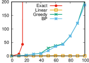
(a) Graph size

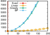
(b) Dataset size

Figure 2: Runtime in milliseconds to (2(a)) compute the graph edit distance between two random graphs; and (2(b)) between all pairs of graphs in a dataset of random graphs.

Figure 2 shows the growth of the runtime with increasing graph and dataset size. Our method is the only one of those studied that scales to large graphs. The number of distance computations and thus the runtime of all methods grows quadratically with the dataset size. Even for the small random graphs on 15 vertices we generated, our method is more than one order of magnitude faster than other approximate methods.

Q2

Greedy vs. Linear

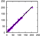
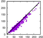
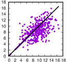
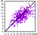
BP vs. Linear

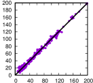
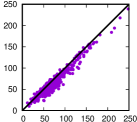
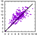
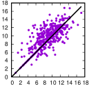
Exact vs. Linear

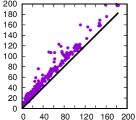
(a) AIDS

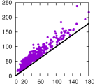
(b) Mutagenicity

(c) Letter (L)

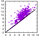
(d) Letter (M)

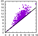
(e) Letter (H)

Figure 3: Graph edit distance computed by Linear ($y$-axis) and Exact/Greedy/BP ($x$-axis) for 500 randomly chosen pairs of graphs from the IAM graph datasets.

Dataset	Accuracy						Runtime
	Exact	BP	Greedy	Linear	GH${}_{\text{SVM}}$	WLOA${}_{\text{SVM}}$	Exact	BP	Greedy	Linear	GH${}_{\text{SVM}}$	WLOA${}_{\text{SVM}}$
AIDS	—	99.6	99.6	99.6	99.5	99.6	—	$2^{\prime}\mkern-1.2mu13^{\prime\prime}\mkern-1.2mu$	$1^{\prime}\mkern-1.2mu35^{\prime\prime}\mkern-1.2mu$	$13^{\prime\prime}\mkern-1.2mu$	$2\text{h\,}2^{\prime}\mkern-1.2mu31^{\prime\prime}\mkern-1.2mu$	$<1^{\prime\prime}\mkern-1.2mu$
Mutag.	—	70.7	70.8	74.4	72.3	80.8	—	$1\text{h\,}21^{\prime}\mkern-1.2mu28^{\prime\prime}\mkern-1.2mu$	$56^{\prime}\mkern-1.2mu37^{\prime\prime}\mkern-1.2mu$	$3^{\prime}\mkern-1.2mu49^{\prime\prime}\mkern-1.2mu$	$>24\text{h\,}$	$19^{\prime\prime}\mkern-1.2mu$
Letter (L)	98.8	98.5	98.7	98.5	98.1	—	$8^{\prime}\mkern-1.2mu19^{\prime\prime}\mkern-1.2mu$	$9^{\prime\prime}\mkern-1.2mu$	$9^{\prime\prime}\mkern-1.2mu$	$4^{\prime\prime}\mkern-1.2mu$	$36^{\prime\prime}\mkern-1.2mu$	—
Letter (M)	93.6	92.9	91.2	91.3	86.0	—	$20^{\prime}\mkern-1.2mu38^{\prime\prime}\mkern-1.2mu$	$10^{\prime\prime}\mkern-1.2mu$	$9^{\prime\prime}\mkern-1.2mu$	$4^{\prime\prime}\mkern-1.2mu$	$36^{\prime\prime}\mkern-1.2mu$	—
Letter (H)	88.4	88.1	87.2	85.2	79.2	—	$40^{\prime}\mkern-1.2mu21^{\prime\prime}\mkern-1.2mu$	$13^{\prime\prime}\mkern-1.2mu$	$12^{\prime\prime}\mkern-1.2mu$	$4^{\prime\prime}\mkern-1.2mu$	$52^{\prime\prime}\mkern-1.2mu$	—
NCI1	—	73.5	74.7	78.1	—	81.5	—	$32^{\prime}\mkern-1.2mu46^{\prime\prime}\mkern-1.2mu$	$26^{\prime}\mkern-1.2mu17^{\prime\prime}\mkern-1.2mu$	$2^{\prime}\mkern-1.2mu7^{\prime\prime}\mkern-1.2mu$	$>24\text{h\,}$	$13^{\prime\prime}\mkern-1.2mu$

TABLE II: Accuracy and runtime for classifying the elements of the test set, including preprocessing if necessary.

To compare how accurately the graph edit distance is computed, we have selected 500 pairs of graphs at random from each IAM dataset and computed their graph edit distance by all four methods. Figure 3 shows how the distance computed by the Linear method compares to the distances obtained by the other three methods. Points below the diagonal line represent pairs of graphs, for which the edit distance computed by Linear is actually smaller than the one computed by the competing approach. Compared to the Greedy approach the Linear method appears to give slightly better results on an average. For the datasets Mutagenicity, Letter (L), (M) and (H) there are more points below the diagonal than above the diagonal. When comparing to BP, this is still the case for the Mutagenicity dataset, but not for the Letter datasets. This can be explained by the fact that continuous distances for several points cannot be represented by a tree metric without distortion. In order to compare with the exact method on Mutagenicity and AIDS, we introduced a timeout of 100 seconds for each distance computation. This was necessary since hard instances may require more than several hours. In case of a timeout the best solution found so far is used, which is not guaranteed to be optimal. The Linear method shows a clear divergence from the solutions of the exact approach, in particular for pairs of graphs with a high (optimal) edit distance. However, it is likely that non-optimal solutions in this case do not harm a nearest neighbours classification.

Q3

Table II summarises the results of the classification experiments. The Linear approach provides a high classification accuracy comparable to BP and Greedy. For the dataset Mutagenicity and NCI1 it even performs better than the other approaches. This can be explained by the ability of the Weisfeiler-Lehman tree to exploit more graph structure than BP. For the Letter datasets, the Linear method is on a par with the other methods for the version with low distortion, but performs slightly worse when the distortion increases. This observation is in accordance with the approximation quality achieved for the datasets, cf. Figure 3. The Linear method clearly outperforms all other approaches in terms of runtime. This becomes in particular clear for the dataset Mutagenicity, which contains the largest graphs in the test with 30.32 vertices on an average.

Q4

The GraphHopper kernel performs worse than our Linear approach w.r.t. running time and classification accuracy. WLOA can only be applied to the molecular datasets with discrete labels. For these it performs exceptionally well regarding both accuracy and runtime. The result suggests that the notion of similarity provided by the graph edit distance is less suitable for this classification task.

VI Conclusion

We have shown that optimal assignments can be computed efficiently for tree metric costs. Although this is a severe restriction, we designed such costs functions suitable for the challenging problem of graph matching. Our approach allows to embed the optimal assignment costs in an $\ell_{1}$ space. It remains future work to exploit this property, e.g., for efficient nearest neighbour search in graph databases.

References

- Garey and Johnson [1979] M. R. Garey and D. S. Johnson, Computers and Intractability: A Guide to the Theory of NP-Completeness. W. H. Freeman, 1979.
- Vishwanathan et al. [2010] S. V. N. Vishwanathan, N. N. Schraudolph, R. I. Kondor, and K. M. Borgwardt, “Graph kernels,” Journal of Machine Learning Research, vol. 11, pp. 1201–1242, 2010.
- Kriege et al. [2019a] N. M. Kriege, F. D. Johansson, and C. Morris, “A survey on graph kernels,” CoRR, vol. abs/1903.11835, 2019. [Online]. Available: https://arxiv.org/abs/1903.11835
- Burkard et al. [2012] R. E. Burkard, M. Dell’Amico, and S. Martello, Assignment Problems. SIAM, 2012.
- Duan and Su [2012] R. Duan and H.-H. Su, “A scaling algorithm for maximum weight matching in bipartite graphs,” in Symposium on Discrete Algorithms. SIAM, 2012, pp. 1413–1424.
- Sharathkumar and Agarwal [2012] R. Sharathkumar and P. K. Agarwal, “A near-linear time -approximation algorithm for geometric bipartite matching,” in ACM Symposium on Theory of Computing. New York, NY, USA: ACM, 2012, pp. 385–394.
- Duan and Pettie [2014] R. Duan and S. Pettie, “Linear-time approximation for maximum weight matching,” J. ACM, vol. 61, no. 1, pp. 1:1–1:23, Jan. 2014.
- Grauman and Darrell [2007] K. Grauman and T. Darrell, “The pyramid match kernel: Efficient learning with sets of features,” J. Mach. Learn. Res., vol. 8, pp. 725–760, May 2007.
- Fröhlich et al. [2005] H. Fröhlich, J. K. Wegner, F. Sieker, and A. Zell, “Optimal assignment kernels for attributed molecular graphs,” in International Conference on Machine learning. New York, NY, USA: ACM, 2005, pp. 225–232.
- Johansson and Dubhashi [2015] F. D. Johansson and D. Dubhashi, “Learning with similarity functions on graphs using matchings of geometric embeddings,” in 21th ACM SIGKDD International Conference on Knowledge Discovery and Data Mining. ACM, 2015, pp. 467–476.
- Kriege et al. [2016] N. M. Kriege, P.-L. Giscard, and R. Wilson, “On valid optimal assignment kernels and applications to graph classification,” in Advances in Neural Information Processing Systems 29, 2016, pp. 1623–1631.
- Conte et al. [2004] D. Conte, P. Foggia, C. Sansone, and M. Vento, “Thirty years of graph matching in pattern recognition,” International Journal of Pattern Recognition and Artificial Intelligence, 2004.
- Foggia et al. [2014] P. Foggia, G. Percannella, and M. Vento, “Graph matching and learning in pattern recognition in the last 10 years,” IJPRAI, vol. 28, no. 1, 2014.
- Kriege et al. [2019b] N. M. Kriege, L. Humbeck, and O. Koch, “Chemical similarity and substructure searches,” in Encyclopedia of Bioinformatics and Computational Biology. Oxford: Academic Press, 2019, pp. 640 – 649.
- Singh et al. [2008] R. Singh, J. Xu, and B. Berger, “Global alignment of multiple protein interaction networks with application to functional orthology detection,” PNAS, vol. 105, no. 35, pp. 12 763–12 768, 2008.
- Zhang and Tong [2016] S. Zhang and H. Tong, “FINAL: Fast attributed network alignment,” in 22nd ACM SIGKDD International Conference on Knowledge Discovery and Data Mining. ACM, 2016, pp. 1345–1354.
- Stauffer et al. [2017] M. Stauffer, T. Tschachtli, A. Fischer, and K. Riesen, “A survey on applications of bipartite graph edit distance,” in Graph-Based Representations in Pattern Recognition. Springer, 2017, pp. 242–252.
- Sanfeliu and Fu [1983] A. Sanfeliu and K.-S. Fu, “A distance measure between attributed relational graphs for pattern recognition.” IEEE Transactions on Systems, Man, and Cybernetics, vol. 13, no. 3, pp. 353–362, 1983.
- Bunke [1997] H. Bunke, “On a relation between graph edit distance and maximum common subgraph,” Pattern Recognition Letters, vol. 18, no. 8, pp. 689–694, 1997.
- Bougleux et al. [2017] S. Bougleux, L. Brun, V. Carletti, P. Foggia, B. Gaüzère, and M. Vento, “Graph edit distance as a quadratic assignment problem,” Pattern Recognition Letters, vol. 87, pp. 38 – 46, 2017.
- Gouda and Hassaan [2016] K. Gouda and M. Hassaan, “CSI_GED: An efficient approach for graph edit similarity computation,” in 32nd IEEE International Conference on Data Engineering, ICDE 2016, Helsinki, Finland, 2016, pp. 265–276.
- Lerouge et al. [2017] J. Lerouge, Z. Abu-Aisheh, R. Raveaux, P. Héroux, and S. Adam, “New binary linear programming formulation to compute the graph edit distance,” Pattern Recognition, vol. 72, no. Supplement C, pp. 254 – 265, 2017.
- Chen et al. [2019] X. Chen, H. Huo, J. Huan, and J. S. Vitter, “An efficient algorithm for graph edit distance computation,” Knowledge-Based Systems, vol. 163, pp. 762 – 775, 2019.
- Lin [1994] C.-L. Lin, “Hardness of approximating graph transformation problem,” in Algorithms and Computation. Springer, 1994, pp. 74–82.
- Riesen and Bunke [2009] K. Riesen and H. Bunke, “Approximate graph edit distance computation by means of bipartite graph matching,” Image and Vision Computing, vol. 27, no. 7, pp. 950–959, 2009.
- Riesen et al. [2015a] K. Riesen, M. Ferrer, R. Dornberger, and H. Bunke, “Greedy graph edit distance,” in Machine Learning and Data Mining in Pattern Recognition, 2015, pp. 3–16.
- Riesen et al. [2015b] K. Riesen, M. Ferrer, A. Fischer, and H. Bunke, “Approximation of graph edit distance in quadratic time,” in Graph-Based Representations in Pattern Recognition. Springer, 2015, pp. 3–12.
- Zeng et al. [2009] Z. Zeng, A. K. H. Tung, J. Wang, J. Feng, and L. Zhou, “Comparing stars: On approximating graph edit distance,” VLDB Endow., vol. 2, no. 1, pp. 25–36, 2009.
- Semple and Steel [2003] C. Semple and M. Steel, Phylogenetics, ser. Oxford lecture series in mathematics and its applications. Oxford University Press, 2003.
- Weisfeiler and Leman [1968] B. Y. Weisfeiler and A. A. Leman, “A reduction of a graph to a canonical form and an algebra arising during this reduction,” Nauchno-Technicheskaya Informatsiya, vol. 2, no. 9, pp. 12–16, 1968, in Russian.
- Arvind et al. [2015] V. Arvind, J. Köbler, G. Rattan, and O. Verbitsky, “On the power of color refinement,” in Fundamentals of Computation Theory. Springer, 2015, pp. 339–350.
- Shervashidze et al. [2011] N. Shervashidze, P. Schweitzer, E. J. van Leeuwen, K. Mehlhorn, and K. M. Borgwardt, “Weisfeiler-lehman graph kernels,” Journal of Machine Learning Research, vol. 12, pp. 2539–2561, 2011.
- Babai et al. [1980] L. Babai, P. Erdős, and S. Selkow, “Random graph isomorphism,” SIAM Journal on Computing, vol. 9, no. 3, pp. 628–635, 1980.
- Steinbach et al. [2000] M. Steinbach, G. Karypis, and V. Kumar, “A comparison of document clustering techniques,” in KDD Workshop on Text Mining, 2000.
- Lloyd [1982] S. Lloyd, “Least squares quantization in pcm,” IEEE Transactions on Information Theory, vol. 28, no. 2, pp. 129–137, March 1982.
- Vattani [2011] A. Vattani, “k-means requires exponentially many iterations even in the plane,” Discrete & Computational Geometry, vol. 45, no. 4, pp. 596–616, Jun 2011.
- Duda et al. [2000] R. O. Duda, P. E. Hart, and D. G. Stork, Pattern Classification. New York, NY, USA: Wiley-Interscience, 2000.
- Aggarwal and Reddy [2013] C. C. Aggarwal and C. K. Reddy, Data Clustering: Algorithms and Applications, 1st ed. Chapman & Hall/CRC, 2013.
- Riesen and Bunke [2008] K. Riesen and H. Bunke, “IAM graph database repository for graph based pattern recognition and machine learning,” in Structural, Syntactic, and Statistical Pattern Recognition, SSPR & SPR. Springer, 2008, pp. 287–297.
- Kersting et al. [2016] K. Kersting, N. M. Kriege, C. Morris, P. Mutzel, and M. Neumann, “Benchmark data sets for graph kernels,” 2016. [Online]. Available: http://graphkernels.cs.tu-dortmund.de
- Feragen et al. [2013] A. Feragen, N. Kasenburg, J. Petersen, M. D. Bruijne, and K. Borgwardt, “Scalable kernels for graphs with continuous attributes,” in Advances in Neural Information Processing Systems 26, 2013, pp. 216–224.
- Chang and Lin [2011] C.-C. Chang and C.-J. Lin, “LIBSVM: A library for support vector machines,” ACM Transactions on Intelligent Systems and Technology, vol. 2, pp. 27:1–27:27, 2011.