Reduced-order Deep Learning for Flow Dynamics

Abstract

In this paper, we investigate neural networks applied to multiscale simulations and discuss a design of a novel deep neural network model reduction approach for multiscale problems. Due to the multiscale nature of the medium, the fine-grid resolution gives rise to a huge number of degrees of freedom. In practice, low-order models are derived to reduce the computational cost. In our paper, we use a non-local multicontinuum (NLMC) approach, which represents the solution on a coarse grid [18]. Using multi-layer learning techniques, we formulate and learn input-output maps constructed with NLMC on a coarse grid. We study the features of the coarse-grid solutions that neural networks capture via relating the input-output optimization to $\ell_{1}$ minimization of PDE solutions. In proposed multi-layer networks, we can learn the forward operators in a reduced way without computing them as in POD like approaches. We present soft thresholding operators as activation function, which our studies show to have some advantages. With these activation functions, the neural network identifies and selects important multiscale features which are crucial in modeling the underlying flow. Using trained neural network approximation of the input-output map, we construct a reduced-order model for the solution approximation. We use multi-layer networks for the time stepping and reduced-order modeling, where at each time step the appropriate important modes are selected. For a class of nonlinear problems, we suggest an efficient strategy. Numerical examples are presented to examine the performance of our method.

1 Introduction

Modeling of multiscale process has been of great interest in diverse applied fields. These include flow in porous media, mechanics, biological applications, and so on. However, resolving the fine-scale features of such processes could be computationally expensive due to scale disparity. Researchers have been working on developing model reduction methods to bridge the information between the scales, in particular, bring the fine-grid information to coarse grid. This generally reduces to constructing appropriate approximation spaces when solving a governing PDEs numerically.

Local model reduction is an important tool in designing reduced-order models for practical applications. Many approaches have been proposed to perform model reduction, which include [3, 24, 5, 23, 15, 10, 11, 21, 2, 20, 26, 27, 34, 32, 29, 14, 17, 12, 13], where the coarse-grid equations are formed and the parameters are computed or found via inverse problems [7, 31, 8, 33, 39]. Adopting upscaling ideas, methods such as Generalized Multiscale Finite Element Method (GMsFEM) [25, 16], Non-local Multicontinuum Methods (NLMC) [19] have been developed. They share similar ideas in constructing the approximation space, where local problems are solved to obtain the basis functions. The numerical solution is then searched within the space that constituted by such basis. With extra local computation, these multiscale spaces can capture the solution using small degrees of freedom. These methods have been proved to be successful in a number of multiscale problems. Global model reduction methods seeks a reduced dimensional solution approximation using global basis functions. When seeking numerical solutions within a high-dimensional approximation space $V_{h}$, the solutions could be sparse. Proper Orthogonal Decomposition (POD) [9] is often used to find a low-dimensional approximate representation of the solutions.

To exploit the advantages of local and global model reduction techniques, global-local model reduction approaches have been explored in the past (see, e.g., [4, 28, 22, 38]). In global-local model reduction methods, the input-output map is approximated using POD or other approaches in combination with multiscale methods. Multiscale methods allow adaptive computing and re-computing global modes [38].

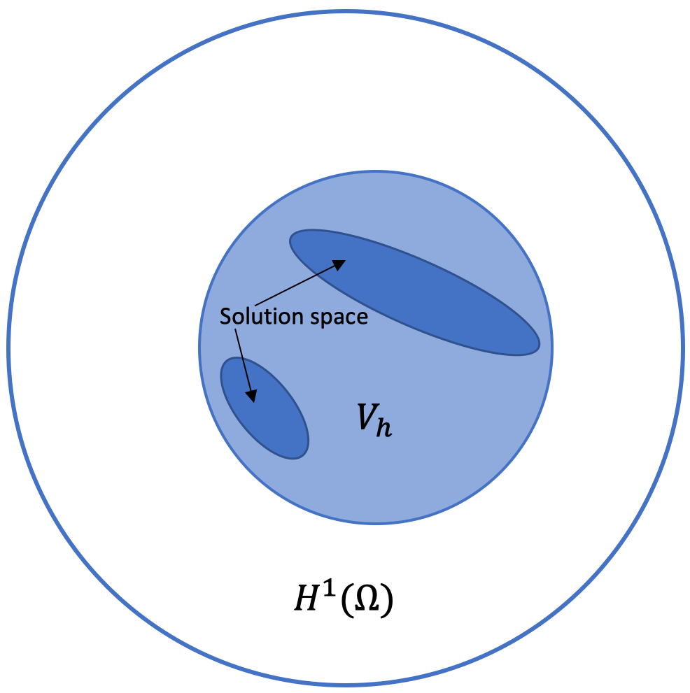
In this paper, we investigate learning strategies for multiscale methods by approximating the input-output map using multi-layer neural networks. Nowadays, neural networks have been commonly used in many applications [36]. In our paper, we use neural networks in conjunction with local reduced-order models. Our studies show that the neural networks provide some type of reduced-order global modes when considering linear problems. In the paper, we investigate these global modes and their relation to spectral modes of input-output map. With a local-global model reduction technique, we limit our search of solution to a smaller zone (see Figure 1 for an illustration) that fits the solution populations better. Our studies show that the multi-layer network provides a good approximation of coarse-grid input-output map and can be used in conjunction with observation data. Moreover, in multi-layer networks, we can learn the forward operators in a reduced way without computing them as in POD like approaches. In our paper, we use multi-layer network for combined time stepping and reduced-order modeling, where at each time step the appropriate important modes are selected. A soft thresholding neural network is suggested based on our analysis.

Figure 1: Illustration of sparsity of our solution.

Our previous work on neural networks and multiscale methods [37] have mostly focused on incorporating the observed data. In this paper, the key tasks are: (1) reproducing the coarse-scale multiscale model; (2) simultaneously determining the sparse representation of solution; and, (3) identifying the dominant multiscale modes and provide a new basis system which can be used to reduce the multiscale model dimension. There are a few advantages of using neural networks to accomplish these tasks. For (1) & (2), the computation is inexpensive and robust. For (3), the dominant multiscale modes found by the neural network can be generalized to conduct model reduction solutions. Our studies suggest the use of soft thresholding and we observe a relation between the soft thresholding and $\ell_{1}$ minimization.

To handle the nonlinearities in PDEs, we propose the use of clustering. Clustering is an effective pretreatment for learning and prediction. Specifically, the solution of nonlinear PDEs clusters around some nonlinear values of the solution (see Figure 1 for an illustration). Sometimes, solution clusters can be predicted without computing solutions. For example, if we are interested in the solutions to the flow equation

$$\dfrac{\partial u}{\partial t}-\text{div}(\kappa(t,x,u)\nabla u)=f,$$ (1)

where $\kappa(t,x,u)=\hat{\kappa}(x)u^{2}$, and $\hat{\kappa}(x)$ has a limited number of configurations as shown in Figure 2, then we could anticipate the solutions to accumulate for each configuration of $\hat{\kappa}(x)$. This is an important example of channelized permeability fields that arise in many subsurface applications. Thus, if we can use this prejudged information and divide the training samples into clusters, we are likely to get an accurate model with significantly less training resources.

Figure 2: Illustration of different configurations of $\hat{\kappa}(x).$

The main contributions of the paper are the following. (1) We study how neural network captures the important multiscale modes related to the features of the solution. (2) We relate $\ell_{1}$ minimization to model reduction and derive a more robust network for our problems using a soft thresholding. (3) We suggest an efficient strategy for some class of nonlinear problems that arise in porous media applications (4) We use multi-layer networks for combined time stepping and reduced-order modeling, where at each time step the appropriate important modes are selected. We remark that we can use observed data to learn multiscale model as in [37].

The paper is organized as follows. Section 2 will be a preliminary introduction of the multiscale problem with a short review on multiscale methods. A description for general neural network is also provided. Section 3 mainly focuses on discussions on the reduced-order neural network. The structure of the neural network is presented. Section4 later discuss the proposed neural network from different aspects and propose a way to conduct model reduction with the neural network coefficient. We also present the relation between the soft thresholding neural network and a $\ell_{1}$ minimization problem in this section. Section 5 provides various numerical examples to verify the predictive power of our proposed neural network and provide support to the claims in Section 4. Lastly, the paper is concluded with Section 6.

2 Preliminaries

2.1 Governing equations and local model reduction

We consider a nonlinear flow equation

$$\dfrac{\partial u}{\partial t}-\text{div}(\kappa(t,x,u)\nabla u)=f,$$ ( 1)

in the domain $(0,T)\times\Omega$. Here, $\Omega$ is the spatial domain, $\kappa$ is the permeability coefficient which can have a multiscale dependence with respect to space and time, and $f$ is a source function. The weak formulation of (1) involves finding $u\in H^{1}(\Omega)$ such that

$$\left(\frac{\partial u}{\partial t},v\right)+(\kappa(t,x,u)\nabla u,\nabla v)=(f,v),\quad\forall v\in H^{1}(\Omega).$$ (2)

If we numerically solve this problem in a $m$-dimensional approximation space $V_{h}\subset H^{1}(\Omega)$, and use an Euler temporal discretization, the numerical solution can be written as

$$u_{h}(t_{n},x)=u_{h}^{n}=\sum_{j=1}^{m}\alpha_{j}^{n}\phi_{j}(x),$$ (3)

where $\{\phi_{j}\}_{j=1}^{m}$ is a set of basis for $V_{h}$. Moreover, the problem (2) can then be reformulated as: find $u_{h}\in V_{h}$ such that

$$\left(\frac{u_{h}^{n+1}-u_{h}^{n}}{\Delta t},v_{h}\right)+(\kappa(t_{n},x,u_{h}^{\nu})\nabla u_{h},\nabla v_{h})=(f,v_{h}),\quad\forall v_{h}\in V_{h},$$ (4)

where $\nu=n$ or $n+1$ corresponds to explicit and implicit Euler discretization respectively. Here, $(\cdot,\cdot)$ denotes the $L_{2}$ inner product.

For problems with multiple scales, a multiscale basis function for each coarse node is computed following the idea of upscaling, i.e., the problem can be solved with a local model reduction. Instead of using the classic piece-wise polynomials as the basis functions, we construct the local multiscale basis following NLMC [37] and use the span of all such basis function as the approximation space $V_{h}$. More specifically, for a fractured media(Figure 3), the basis functions of (1) can be constructed by the following steps:

• Step 1: Partition of domain

  $$\Omega=\Omega_{m}\bigoplus_{n}d_{n}\Omega_{f,n}.$$ (5)

  Assume $\mathcal{T}^{H}$ is a coarse-grid partition of the domain $\Omega$ with a mesh size $H$ which is further refined into a fine mesh $\mathcal{T}^{h}$. Denote by $\{K_{i}|\quad i=1,\cdots,N\}$ the set of coarse elements in $\mathcal{T}^{H}$, where $N$ is the number of coarse blocks. We also define the oversampled region $K^{+}_{i}$ for each $K_{i}$, with a few layers of neighboring coarse blocks, see Figure 3 for the illustration of $K_{i}$ and $K_{i}^{+}$. We further define the set of all fracture segments within a coarse block $K_{j}$ as $F^{j}=\{f_{n}^{(j)}|1\leq n\leq L_{j}\}=\{\cup_{n}\Omega_{f,n}\}\cap K_{j}$ and $L_{j}=dim\{F^{j}\}$.

  

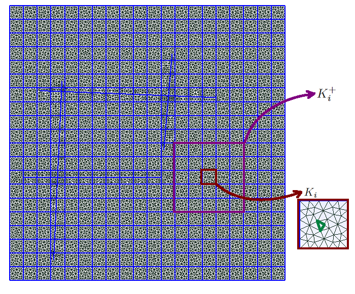
  Figure 3: Illustration of coarse and fine meshes.

• Step 2: Computation of local basis function in $K_{i}^{+}$.

  The basis for each over-sampled region $\psi_{m}^{(i)}$ solves the following local constraint minimizing problem on the fine grid

  $$a(\psi_{m}^{(i)},v)+\sum_{K_{j}\subset K_{i}^{+}}\left(\mu_{0}^{(j)}\int_{K_{j}}v+\sum_{1\leq m\leq L_{j}}\mu_{m}^{(j)}\int_{f_{m}^{(j)}}v\right)=0,\quad\forall v\in V_{0}(K_{i}^{+}),$$ (6)

  $$\int_{K_{j}}\psi_{m}^{(i)}=\delta_{ij}\delta_{0m},\quad\forall K_{j}\subset K_{i}^{+},$$

  $$\int_{f_{n}^{(j)}}\psi_{m}^{(i)}=\delta_{ij}\delta_{nm},\quad\forall f_{n}^{(j)}\in F^{(j)},\;\forall K_{j}\subset K_{i}^{+},$$

  where $a(u,v)=\int_{D_{m}}\kappa_{m}\nabla u\cdot\nabla v+\sum_{i}\int_{D_{f,i}}\kappa_{i}\nabla_{f}u\cdot\nabla_{f}v$, $\mu_{0}^{(j)},\mu_{m}^{(j)}$ are Lagrange multipliers while $V_{0}(K_{i}^{+})=\{v\in V(K^{+}_{i})|v=0\text{ on }\partial K_{i}^{+}\}$ and $V(K_{i}^{+})$ is the fine grid space over an over-sampled region $K^{+}_{i}$. By this way of construction, the average of the basis $\psi_{0}^{(i)}$ equals $1$ in the matrix part of coarse element $K_{i}$, and equals $0$ in other parts of the coarse blocks $K_{j}\subset K_{i}^{+}$ as well as any fracture inside $K_{i}^{+}$. As for $\psi_{m}^{(i)},m\geq 1$, it has average $1$ on the $m$-th fracture continua inside the coarse element $K_{i}$, and average $0$ in other fracture continua as well as the matrix continua of any coarse block $K_{j}\subset K_{i}^{+}$. It indicates that the basis functions separate the matrix and fractures, and each basis represents a continuum.

The resulting multiscale basis space is finally written as $V_{h}=span\{\psi_{m}^{(i)}|0\leq m\leq L_{i},1\leq i\leq N\}$. By renumbering the basis, we denote all basis function as $\{\phi_{j}\}_{j=1}^{m}$, where $m=\sum_{i=1}^{N}(L_{j}+1)$.

Thus, the coefficient $U^{n}=(\alpha_{1}^{n},\alpha_{2}^{n},\ldots,\alpha_{m}^{n})^{T}$ satisfies the recurrence relation

$$U^{n+1}=(M+\Delta tA^{\nu})^{-1}(MU^{n}+\Delta tF^{n}),$$ (7)

where $M$ and $A^{\nu}$ are the mass matrix and the stiffness matrix with respect to the basis $\{\phi_{j}\}_{j=1}^{m}$, $\nu$ can be $n$ or $n+1$ depending on the temporal scheme that we use. We have

$$\begin{split}[M]_{ij}&=\int_{\Omega}\phi_{i}(x)\phi_{j}(x)\,dx,\\ [A^{\nu}]_{ij}&=\int_{\Omega}\kappa(t_{n},x,u^{\nu}_{h})\nabla\phi_{i}(x)\cdot\nabla\phi_{j}(x)\,dx.\end{split}$$

We claim that a global model reductions can be conducted to the problem described above, as solution $u_{h}^{n}(x)$ in many cases can be sparse in $V_{h}$ even if $V_{h}$ is a reduced-order space. For instance, $u_{h}(t_{n},x)$ is strongly bonded to initial condition $u_{h}(t_{0},x)$. It can be foreseen that if initial conditions are chosen from a small subspace of $V_{h}(\Omega)$, $u_{h}^{n}(x)=u_{h}(t_{n},x)$ is also likely to accumulate somewhere in $V_{h}$. In other words, the distribution of coefficients $U^{n}$ can hardly expand over the entire $\mathbb{R}^{m}$ space but only lies in a far smaller subspace.

Other physical restrictions to the problem could also narrow down the space of solution. This indicates that $u_{h}(t_{n},x)$ can be closely approximated with less degrees of freedom. Section 3 and Section 4 will be discussing how to identify dominant modes in the space of $U^{n}$ using a neural network.

2.2 Neural Network

A neural network is usually used to learn a map from existing data. For example, if we are given samples $\{(x_{i},y_{i})\}_{i=1}^{L}$ from the map $\mathcal{F}:X\to Y$, i.e., $\mathcal{F}(x_{i})=y_{i}$ for $1\leq i\leq L$, and we would like to predict the value of $\mathcal{F}(x_{i})$ for $i=L+1,\cdots,L+M$. With the help of neural network, this problem can be reformulated as the optimization problem. The optimization takes $\{(x_{i},y_{i})\}_{i=1}^{L}$ as training samples and produces a proper network coefficient $\theta^{*}$ starting from some initialization chosen at random. More specifically, if the neural network $\mathcal{NN}(\cdot)$ has a feed-forward fully-connected structure, then

$$\mathcal{NN}(x;\theta)=W_{n}\sigma(\cdots\sigma(W_{2}\sigma(W_{1}x+b_{1})+b_{2})\cdots)+b_{n}.$$ (8)

Here, $\theta$ represents all tuneable coefficients in neural network $\mathcal{NN}(\cdot)$ and $\sigma(\cdot)$ is some nonlinear activation function. There are many choices of such nonlinear functions [35], while the most common ones used are ReLU and $\tanh$.

For the network defined above, $\theta$ is indeed defined as $\theta=\{W_{1},b_{1},W_{2},b_{2},\cdots,W_{n},b_{n}\}$. We will use the output $\mathcal{NN}(x_{i})$ to approximate the desired output $y_{i}$. The difference between them will be measured using a cost function $\mathcal{C}(\cdot)$. For example, we can take the mean square error and the loss function is defined as

$$\mathcal{C}(\theta)=\frac{1}{N}\sum_{i=1}^{N}(y_{i}-\mathcal{NN}(x_{i}))^{2},$$ (9)

which measures the average squared difference between the estimated values and the observed values. The neural network is then optimized by seeking $\theta^{*}$ to minimize the loss function.

$$\theta^{*}=\operatorname*{\text{argmin}}_{\theta}\mathcal{C}(\theta).$$ (10)

Numerically, this optimization problem can be solved with a stochastic gradient descent(SGD) type method [30]. By calculating the gradient of the loss function, the coefficient $\theta$ is iteratively updated in an attempt to minimize the loss function. This process is also referred as “training”. Once the loss is minimized to a satisfactory small level, the neural network parameters $\theta^{*}$ is decided, and further, the overall neural network architecture (15) is constructed. The predictions can then be given as $\mathcal{NN}(x_{i};\theta^{*})$ for $i=L+1,\cdots,L+M$.

3 Reduced-order neural network

In this section, we present the construction of reduced-order neural network. We propose a reduced-order neural network that can model a time series. Moreover, if there exists a basis that approximates the solution for each time step with sparse coefficients, then the proposed neural network can identify such basis from the training samples. Specifically, Subsection 3.1 will discuss the macroscopic structure of the proposed neural network while Subsection 3.2 will discuss two designs of the sub-network of the network with more details. Subsection 3.3 later assembles the full multi-layer neural network.

3.1 Reduced-order neural network structure

We propose a reduced-order neural network as shown in Figure 4(a). Here, the full network is constituted by several sub-networks. Each sub-network $\mathcal{N}^{n}(\cdot)$ is expected to model a one-step temporal evolution from $\mathbf{x}^{n}$ to $\mathbf{x}^{n+1}$ in a time series $\vec{\mathbf{x}}=[\mathbf{x}^{0},\mathbf{x}^{1},\cdots,\mathbf{x}^{n}]$.

Sub-networks should have a general structure as shown in Figure 4(b). The specific design will vary depending on the problem we are modeling (see discussions in Subsection 3.2). The sub-network is built in a way that the input $\mathbf{x}^{n}$ will be first feed into a multi-layer fully-connected network named as “operation layer”. This layer is intended for the neural network to capture the map between two consecutive time steps. The output of the operation layer is then fed into a soft thresholding function to impose sparsity to the solution coefficient. Lastly, the data will be processed with a “basis transform layer” in which a new basis set will be learned. With the basis set, one can represent the solution with sparse coefficients assuming such representation exists.

(a) Multi-layer reduced-order neural network $\mathcal{NN}(\cdot)$

(b) Sub-network $\mathcal{N}^{n}(\cdot)$

Figure 4: Reduced-order neural network structure.

3.2 Sub-network

In this subsection, we present two designs of the sub-network $\mathcal{N}^{n}(\cdot)$. One is for modeling linear dynamics while the other is designed for nonlinear dynamics. One can choose from these two options when assembling the full network depending on the dynamics of interest. Both sub-network designs are intended to learn a new set of basis and then impose the sparsity to the solution coefficient in the new system while learning dynamics.

3.2.1 Sub-network for linear process

We first present the sub-network for modeling linear dynamics. It can be used to model the one-step flow described in (1), where we define the sub-network for the $n$-th time step as

$$\mathcal{N}^{n}(\mathbf{x}^{n};\theta_{n}):=W_{n}^{2}S_{\gamma}(W_{n}^{1}\cdot\mathbf{x}^{n}+b_{n}).$$ (11)

Here, for the sub-network parameter $\theta_{n}=(W_{n}^{1},W_{n}^{2},b_{n})$, $W_{n}^{1}$ and $b_{n}$ are in the operation layer and $W_{n}^{2}$ works as the basis transformation layer. $S_{\gamma}$ is the soft thresholding function defined point-wise as $S_{\gamma}:\mathbb{R}\to\mathbb{R}$

$$S_{\gamma}(x)=\text{sign}(x)(|x|-\gamma)_{+}\begin{cases}x-\gamma&\text{ if }x\geq\gamma,\\ 0&\text{ if }-\gamma<x<\gamma,\\ x+\gamma&\text{ if }x\leq-\gamma.\end{cases}$$ (12)

We further require $W_{n}^{2}$ to be an orthogonal matrix, i.e. $(W_{n}^{2})^{T}\cdot(W_{n}^{2})=I$. To this end, we train the network (11) with respect to the cost function

$$\mathcal{C}^{n}(\theta_{n})=\|\mathbf{x}^{n+1}-\mathcal{N}^{n}(\mathbf{x}^{n};\theta_{n})\|_{2}^{2}+\eta_{n}\|(W_{n}^{2})^{T}\cdot(W_{n}^{2})-I\|_{1}$$ (13)

with a penalty on the orthogonality constraint of $W_{n}^{2}$. $\eta$ is a hyper coefficient for adjusting the weight of the $\ell_{1}$ regularization term. Here, $\mathbf{x}^{n}$ is the input of $\mathcal{N}^{n}(\cdot;\theta_{n})$, and $\mathcal{C}^{n}(\cdot)$ measures the mismatch between true solution $\mathbf{x}^{n+1}$ and the prediction $\mathcal{N}^{n}(\mathbf{x}^{n})$ while forcing $W_{n}^{2}$ to be orthogonal. We remark that this cost functions is only a part of the full cost function that we will be discussed in Subsection 3.3.

With such a design, the trained neural sub-network $\mathcal{N}^{n}(\cdot;\theta_{n}^{*})$ will be able to model the input-output map specified by the training data while producing a matrix $W^{2}_{n}$ whose columns forms an orthogonal basis in $\mathbb{R}^{m}$.

3.2.2 Sub-network for nonlinear process

Similar to the linear case, a sub-network for nonlinear process can also be designed. When the output $\mathbf{x}^{n+1}$ is non-linearly dependent on input $\mathbf{x}^{n}$, we make use of a $d_{n}$-layer feed-forward neural network $\tilde{\mathcal{N}}(\cdot)$ to approximate the input-output map. $\tilde{\mathcal{N}}(\cdot)$ will work as the operation layer of the sub-network. The output of $\tilde{\mathcal{N}}(\cdot)$ is then processed with soft-thresholding and a basis transformation layer $W_{n}^{2}$. We define the sub-network to be

$$\begin{split}\mathcal{N}^{n}(\mathbf{x}^{n};\theta_{n})&:=W_{n}^{2}S_{\gamma}(\tilde{\mathcal{N}}(\mathbf{x}^{n};\theta_{n})),\\ \tilde{\mathcal{N}}(\mathbf{x}^{n};\theta_{n})&:=W_{n}^{1,d_{n}}(\cdots(\sigma(W_{n}^{1,3}\sigma(W_{n}^{1,2}\sigma(W_{n}^{1,1}\mathbf{x}^{n}+b_{n}^{1})+b_{n}^{2})\cdots+b_{n}^{d_{n}}),\end{split}$$ (14)

where $\theta_{n}=\left(W_{n}^{1,1},W_{n}^{1,2},\ldots,W_{n}^{1,d_{n}},W_{n}^{2},b_{n}^{1},b_{n}^{2},\ldots,b_{n}^{d_{n}}\right)$ is the sub-network parameter, and $\sigma(\cdot)$ is a nonlinear activation function. The cost function for training the sub-network parameter is again defined in (13). We also remark that if $d_{n}=1$ and $\sigma=\mathbf{1}$ is the point-wise identify function, then the network structure (14) is reduced to (11).

Another approach to reduce the difficulty of reproducing a nonlinear process is clustering. Instead of using a single network to approximate complicated nonlinear relations, we use different networks for different data cluster. As discussed in the Section 1, the clusters of the solutions can be predicted. Thus, separate the training samples by cluster can be an easy and effective way to accurately recover complicated process. Discussions on clustering and numerical examples are presented in Section 5.5.

3.3 Multi-layer reduced order network

Now we construct the full neural network $\mathcal{NN}(\cdot;\theta)$ by stacking up the sub-network $\mathcal{N}^{n}(\cdot;\theta_{n})$. More precisely, $\mathcal{NN}(\cdot;\theta):\mathbb{R}^{m}\to\mathbb{R}^{m}$ is defined as:

$$\mathcal{NN}(\mathbf{x}^{0};\theta):=\mathcal{N}^{n}(\cdots\mathcal{N}^{1}(\mathcal{N}^{0}(\mathbf{x}^{0};\theta_{0});\theta_{1})\cdots;\theta_{n}),$$ (15)

where $\mathcal{N}^{n}(\cdot;\theta_{n})$ is defined as in (11) or (14) depending the linearity of the process, and $\theta=(\theta_{0},\theta_{1},\ldots,\theta_{n})$ is the full network parameter. We use such $\mathcal{NN}(\cdot;\theta)$ to approximate time series $\vec{\mathbf{x}}=[\mathbf{x}^{0},\mathbf{x}^{1},\cdots,\mathbf{x}^{n+1}]$. Denote the output of $(t+1)$-fold composition of sub-network $\mathcal{N}^{t}$ as

$$\mathbf{o}^{t+1}:=\mathcal{N}^{t}(\cdots\mathcal{N}^{1}(\mathcal{N}^{0}(\mathbf{x}^{0};\theta_{0});\theta_{1})\cdots;\theta_{t}).$$ (16)

Then $\mathbf{o}^{t+1}$ works as a prediction of the solution at time $t+1$. The full cost function is then defined as

$$\mathcal{C}(\theta)=\sum_{t=0}^{n}\|\mathbf{o}^{t+1}-\mathbf{x}^{t+1}\|_{2}^{2}+\eta_{t}\|(W_{t}^{2})^{T}\cdot(W_{t}^{2})-I\|_{1},$$ (17)

where $\vec{\mathbf{x}}$ is the true time sequence, and $\eta_{t}$ is hyper-parameter stands for the weight of the regularizer while $\theta$ represents all tuneable parameters of $\mathcal{NN}(\cdot)$. Each layer (sub-network) corresponds to a one-step time evolution of the dynamics.

Suppose we have $L$ training samples,

$$\vec{\mathbf{x}_{i}}=[(\mathbf{x}_{i}^{0}),(\mathbf{x}_{i}^{1},\mathbf{x}_{i}^{2},\cdots,\mathbf{x}_{i}^{n+1})],\quad\quad 1\leq i\leq L.$$

The optimal parameter $\theta^{*}$ of $\mathcal{NN}(\cdot)$ is then determined by optimizing the cost function $\mathcal{C}(\theta)$ subject to this training set $\{\vec{\mathbf{x}_{i}}\}_{i=1}^{L}$ as discussed Section 2.2. Once $\theta^{*}$ is decided, predictions can be made for testing samples $[\mathbf{x}_{i}^{1},\cdots,\mathbf{x}_{i}^{n+1}]$ by $\mathcal{NN}(\mathbf{x}_{i}^{0}),i>L.$

4 Discussions and applications

In this section, we discuss some theoretical aspects of proposed neural networks. Specifically, we use the proposed network to model fluid dynamics in heterogeneous media, as described in (1). First, we relate the soft thresholding network with $\ell_{1}$ optimization problem. Secondly, we explore how learned coefficients of neural network are related to the map that is being approximated. Thirdly, based on the understanding of proposed neural network, we present a way to utilize the trained network coefficient to construct a reduced-order model.

Specifically, we consider a one-layer neural network for single-step linear dynamics

$$\mathcal{NN}(\mathbf{x};\theta)=\mathcal{N}(\mathbf{x};\theta):=W^{2}S_{\gamma}(W^{1}\mathbf{x}+b),$$ (18)

omitting the indices for time step $n$. We train the neural network $\mathcal{NN}(\cdot;\theta)$ with data pairs $\{(U_{i}^{n},U_{i}^{n+1})\}_{i=1}^{L}$, which are NLMC solution coefficients (see Section 2.1 for more details details of data generation) to (1) at $t^{n}$ and $t^{n+1}$, respectively. More precisely, we consider the linear case of (1), when $\kappa(t,x)$ is independent of $u_{h}^{n}$. In this case, the one step fluid dynamics (7) is indeed a linear revolution such that $A^{n}$ is only dependent on time. Further, we denote $\hat{W_{n}}$ and $\hat{b_{n}}$ by

$$\begin{split}\hat{W}&=(M+\Delta tA^{n})^{-1}M,\\ \hat{b}&=(M+\Delta tA^{n})^{-1}\Delta tF^{n}.\\ \end{split}$$ (19)

Then

$$U^{n+1}_{i}=\hat{W}U^{n}_{i}+\hat{b},\quad 1\leq i\leq L,$$ (20)

for all training samples that we use in this section. We further define the linear map between $U^{n}_{i}$ and $U_{i}^{n+1}$ as $\mathcal{\hat{L}}(\cdot):\mathbb{R}^{m}\to\mathbb{R}^{m}$

$$\mathcal{\hat{L}}(\mathbf{x}):={\hat{W}}\mathbf{x}+{\hat{b}}.$$ (21)

From now on, when there is no risk of confusion, we drop the optimal network parameter $\theta^{*}$ in the trained network $\mathcal{NN}(\cdot)$. fz We expect $\mathcal{NN}(\cdot)$ to learn the map $\mathcal{\hat{L}}(\cdot)$ from the data while extracting a system $W^{2}$ in which the data $U^{n+1}_{i}$ can be represented sparsely.

4.1 Sparsity and $\ell_{1}$ minimization

To understand the trained neural network $\mathcal{NN}(\cdot)$, we first assume the following.

Assumption 1.

For a subspace $S\subset\mathbb{R}^{m}$, there exist some orthogonal matrix $\hat{W}^{2}\in\mathbb{R}^{m\times m}$ such that $(\hat{W}^{2})^{T}\mathcal{\hat{L}}(\mathbf{x})$ can be approximated by a sparse vector in $\mathbb{R}^{m}$ for any $\mathbf{x}\in S$. More precisely, there exist an approximation error function $\epsilon(\cdot):\mathbb{N}\to\mathbb{R}^{+}$, such that for any $\mathbf{x}\in S$, there exist a corresponding $s$-sparse vector $\mathbf{y}_{s}\in\mathbb{R}^{m}$ satisfies

$$\|(\hat{W}^{2})^{T}\mathcal{\hat{L}}(\mathbf{x})-\mathbf{y}_{s}\|_{2}\leq\epsilon(s).$$ (22)

We then take $\{U_{i}^{n}\}_{i=1}^{L}$ from $S$ and define $U^{n+1,\hat{W}^{2}}_{i}:=(\hat{W}^{2})^{T}U^{n+1}_{i}$ for all training pairs$(U_{i}^{n},U_{i}^{n+1})$ of $\mathcal{NN}(\cdot)$. By Assumption 1, there exist $s$-sparse vector $U^{s}_{i}\in\mathbb{R}^{m}$ such that

$$||U^{n+1,\hat{W}^{2}}_{i}-U^{s}_{i}||_{2}\leq\epsilon(s)$$ (23)

for $1\leq i\leq L$.

Additionally, for any orthogonal matrix $W^{2}\in\mathbb{R}^{m\times m}$, we denote define $U_{i}^{n+1,{W}^{2}}:=(W^{2})^{T}U_{i}^{n+1}$ and denote it as $[\alpha_{i,1}^{n+1,W^{2}},\alpha_{i,2}^{n+1,W^{2}},\cdots,\alpha_{i,m}^{n+1,W^{2}}]^{T}$. Recall (3), and the corresponding numerical solution $u_{h,i}^{n+1}$ at time step $n+1$ can be written as

$$u_{h,i}^{n+1}=\Phi U^{n+1}_{i},$$

letting $\Phi=[\phi_{1},\phi_{2},\cdots,\phi_{m}]$ be the multiscale basis functions, and $U^{n+1}_{i}$ be the corresponding coefficient vector. By the orthogonality of $W^{2}$, $u_{h,i}^{n+1}$ can be further written as

$$u_{h,i}^{n+1}=\Phi(W^{2})U^{n+1,W^{2}}_{i}=\Phi^{W^{2}}U_{i}^{n+1,W^{2}},$$ (24)

with $\Phi^{W^{2}}$ defined as

$$\Phi^{W^{2}}:=\Phi W^{2}.$$ (25)

We further denote the columns of $\Phi^{W^{2}}$ as $\phi^{W^{2}}_{j}$’s. Then $\{\phi^{W^{2}}_{j}\}_{j=1}^{m}$ is actually a new set of multiscale basis functions such that $u_{h,i}^{n+1}$ can be written as

$$u_{h,i}^{n+1}=\sum_{j=1}^{m}\alpha_{i,j}^{n+1,W^{2}}\phi^{W^{2}}_{j}.$$ (26)

If $W^{2}$ is taken to be $\hat{W}^{2}$ as in Assumption 1, we will obtain

$$u_{h,i}^{n+1}=\sum_{j=1}^{m}\alpha_{i,j}^{n+1,\hat{W}^{2}}\phi^{\hat{W}^{2}}_{j},$$

where the coefficient $U^{n+1,\hat{W}^{2}}_{i}=[\alpha_{i,1}^{n+1,\hat{W}^{2}},\alpha_{i,2}^{n+1,\hat{W}^{2}},\cdots,\alpha_{i,m}^{n+1,\hat{W}^{2}}]^{T}$ can be closely approximated by a sparse vector $U_{i}^{s}$.

We then claim that our proposed neural network $\mathcal{NN}(\cdot)$ is able to approximate such $\hat{W}^{2}$ and a sparse approximation of the output from data. This is guaranteed by the following lemma from [6]:

Lemma 4.1.

We define $\mathcal{\hat{N}}(\cdot),\mathbb{R}^{m}\to\mathbb{R}^{m}$ as

$$\mathcal{\hat{N}}(\mathbf{x}):=S_{\gamma}(W\mathbf{x}+b).$$

The output of $\mathcal{\hat{N}}(\mathbf{x})$ is the solution of the $\ell_{1}$-regularized problem

$$\mathbf{y}^{*}=\operatorname*{\text{argmin}}_{\mathbf{y}\in\mathbb{R}^{m}}\dfrac{1}{2}\|\mathbf{y}-({W}\mathbf{x}+{b})\|_{2}^{2}+\gamma\|\mathbf{y}\|_{1}$$ (27)

by proximal gradient update.

Proof.

It is straightforward to see that the directional derivative of the residual with respect to $\mathbf{y}$ is given by $\mathbf{y}-({W}\mathbf{x}+{b})$. On the other hand, the soft thresholding operator is the proximal operator of the $\ell_{1}$ norm, i.e.

$$S_{\gamma}(x)=\text{prox}_{\gamma\|\cdot\|_{1}}(\mathbf{x})=\operatorname*{\text{argmin}}_{\mathbf{y}\in\mathbb{R}^{m}}\left(\dfrac{1}{2}\|\mathbf{y}-\mathbf{x}\|_{2}^{2}+\gamma\|\mathbf{y}\|_{1}\right).$$

With a zero initial guess, the 1-step proximal gradient update of (27) with a step size $\gamma$ is therefore

$$\begin{split}\mathbf{y}^{*}=\mathcal{\hat{N}}(\mathbf{x})=S_{\gamma}({W}\mathbf{x}+{b}).\end{split}$$

∎

Thus, for the one-step neural network $\mathcal{NN}(\cdot)$ defined in (18), Lemma 4.1 implies that

$$\mathcal{NN}(\mathbf{x})=\operatorname*{\text{argmin}}_{\mathbf{y}\in\mathbb{R}^{m}}\dfrac{1}{2}\|\mathbf{y}-W^{2}W^{1}\mathbf{x}+W^{2}b\|_{2}^{2}+\gamma\|(W^{2})^{T}\mathbf{y}\|_{1}.$$ (28)

That is to say, the output of the trained neural network $\mathcal{NN}(\cdot)$ is actually the solution to a $\ell_{1}$ optimization problem. We further define the linear operator$\mathcal{{L}}(\cdot):\mathbb{R}^{m}\to\mathbb{R}^{m}$ as

$$\mathcal{{L}}(\mathbf{x}):=W^{2}W^{1}\mathbf{x}+W^{2}b.$$ (29)

Equation actually (28) implies that

$$\mathcal{L}(\cdot)\approx\mathcal{NN}(\cdot)$$ (30)

as $\mathcal{NN}(\mathbf{x})$ minimizes $\|\mathbf{y}-W^{2}W^{1}\mathbf{x}+W^{2}b\|_{2}^{2}$. Moreover, the output of $\mathcal{NN}(\cdot)$ is sparse in the coordinate system $W^{2}$ as it also minimized the $\|(W^{2})^{T}\mathbf{y}\|_{1}$ term.

$S_{\gamma}$ is widely used in $\ell_{1}$-type optimization for promoting sparsity and extracting important features as discussed above. It is therefore also brought into network to extract sparsity from the training data. For other network defined with activation functions such as ReLU, we also remark there’s an correlation between $S_{\gamma}$ and ReLU. Recall its definition in (12) :

$$S_{\gamma}(x)=\text{sign}(x)(|x|-\gamma)_{+}\begin{cases}x-\gamma&\text{ if }x\geq\gamma,\\ 0&\text{ if }-\gamma<x<\gamma,\\ x+\gamma&\text{ if }x\leq-\gamma.\end{cases}$$

and that of $\text{ReLU}:\mathbb{R}\to\mathbb{R}$

$$\text{ReLU}(x)=\max\{x,0\}=\begin{cases}x&\text{ if }x\geq 0,\\ 0&\text{ if }x<0.\end{cases}$$

We have the following:
One can explicitly represent the soft thresholding operator $S_{\gamma}$ by the ReLU function as

$$S_{\gamma}(x)=\text{ReLU}(x-\gamma)-\text{ReLU}(-x-\gamma)\quad\forall x\in\mathbb{R},$$ (31)

or in an entry-wise sense, one can write

$$S_{\gamma}(\mathbf{x})=J_{m}\text{ReLU}(J_{m}^{T}\mathbf{x}-\gamma\mathbf{1}_{2m})\quad\forall\mathbf{x}\in\mathbb{R}^{m},$$ (32)

where $J_{m}=[I_{m},-I_{m}]$. Activation functions $S_{\gamma}(\cdot)$ can thus be easily implemented with the help of ReLU. Further, it also means that our proposed neural network is only a special class of neural networks that are defined with ReLU.

4.2 linear operator $\mathcal{\hat{L}}\approx\mathcal{NN}$

For neural network $\mathcal{NN}(\cdot)$ as defined in (18)

$$\mathcal{NN}(\mathbf{x})=W^{2}S_{\gamma}(W^{1}\mathbf{x}+b),$$

we claim the following

Lemma 4.2.

We assume Assumption 1 holds. There exist a set of parameters $(W^{1},W^{2},b)\in\mathbb{R}^{m\times m}\times\mathbb{R}^{m\times m}\times\mathbb{R}^{m}$ such that

$$\|\mathcal{NN}(\mathbf{x})-\mathcal{\hat{L}}(\mathbf{x})\|_{2}\leq 2\epsilon(s)+s^{\frac{1}{2}}\gamma,\;\quad\forall x\in S.$$ (33)

Proof.

By Assumption 1, there exist some orthogonal matrix $\hat{W}^{2}\in\mathbb{R}^{m\times m}$ such that for all $\mathbf{x}\in S$, we have

$$\|(\hat{W}^{2})^{T}\mathcal{\hat{L}}(\mathbf{x})-\mathbf{y}_{s}\|_{2}\leq\epsilon(s),$$ (34)

where $\mathbf{y}_{s}$ is an $s$-sparse vector. Next, we consider $W^{1}=(\hat{W}^{2})^{T}\hat{W}$, $W^{2}=\hat{W}^{2}$ and $b=(\hat{W}^{2})^{T}\hat{b}$. We recall the definition of $\mathcal{\hat{L}}(\cdot)$

$$\mathcal{\hat{L}}(\mathbf{x}):={\hat{W}}\mathbf{x}+{\hat{b}}.$$

The difference between $\mathcal{NN}(\mathbf{x})$ and $\hat{\mathcal{L}}(\mathbf{x})$ can then be estimated by

$$\|\mathcal{NN}(\mathbf{x})-\hat{\mathcal{L}}(\mathbf{x})\|_{2} =\|\hat{W}^{2}S_{\gamma}\Big{(}(\hat{W}^{2})^{T}\hat{W}\mathbf{x}+(\hat{W}^{2})^{T}\hat{b}\Big{)}-\hat{\mathcal{L}}(\mathbf{x})\|_{2}$$

$$=\|\hat{W}^{2}\Big{(}S_{\gamma}\Big{(}(\hat{W}^{2})^{T}\hat{W}\mathbf{x}+(\hat{W}^{2})^{T}\hat{b}\Big{)}-(\hat{W}^{2})^{T}\mathcal{\hat{L}}(\mathbf{x})\Big{)}\|_{2}$$

$$=\|\hat{W}^{2}\Big{(}S_{\gamma}\Big{(}(\hat{W}^{2})^{T}\mathcal{\hat{L}}(\mathbf{x})\Big{)}-(\hat{W}^{2})^{T}\mathcal{\hat{L}}(\mathbf{x})\Big{)}\|_{2}$$

$$=\|S_{\gamma}\Big{(}(\hat{W}^{2})^{T}\mathcal{\hat{L}}(\mathbf{x})\Big{)}-(\hat{W}^{2})^{T}\hat{\mathcal{L}}(\mathbf{x})\|_{2}.$$

Since $|S_{\gamma}(z_{2})-S_{\gamma}(z_{1})|\leq|z_{2}-z_{1}|,\;\forall z_{1},z_{2}\in\mathbb{R}$, we have

$$\|S_{\gamma}\Big{(}(\hat{W}^{2})^{T}\mathcal{\hat{L}}(\mathbf{x})\Big{)}-S_{\gamma}(\mathbf{y}_{s})\|_{2}\leq\|(\hat{W}^{2})^{T}\mathcal{\hat{L}}(\mathbf{x})-\mathbf{y}_{s}\|_{2}\leq\epsilon(s).$$

Thus, we obtain

$$\|S_{\gamma}\Big{(}(\hat{W}^{2})^{T}\mathcal{\hat{L}}(\mathbf{x})\Big{)}-(\hat{W}^{2})^{T}\hat{\mathcal{L}}(\mathbf{x})\|_{2}$$

$$\leq \|S_{\gamma}\Big{(}(\hat{W}^{2})^{T}\mathcal{\hat{L}}(\mathbf{x})\Big{)}-S_{\gamma}(\mathbf{y}_{s})\|_{2}+\|S_{\gamma}(\mathbf{y}_{s})-\mathbf{y}_{s}\|_{2}+\|\mathbf{y}_{s}-(\hat{W}^{2})^{T}\hat{\mathcal{L}}(\mathbf{x})\|_{2}$$

$$\leq 2\epsilon(s)_{+}\|\mathbf{y}_{s}-S_{\gamma}(\mathbf{y}_{s})\|.$$

Since $|(S_{\gamma}(\mathbf{y}_{s})-\mathbf{y}_{s})_{i}|\leq\gamma$, we have

$$\|S_{\gamma}(\mathbf{y}_{s})-\mathbf{y}_{s}\|_{2}^{2}=\sum_{(\mathbf{y}_{s})_{i}\neq 0}|(S_{\gamma}(\mathbf{y}_{s})-\mathbf{y}_{s})_{i}|^{2}\leq s\gamma^{2},$$

and therefore we have

$$\|\mathcal{NN}(\mathbf{x})-\hat{\mathcal{L}}(\mathbf{x})\|_{2}\leq 2\sigma(s)+s^{\frac{1}{2}}\gamma,$$

letting $W^{1}=(\hat{W}^{2})^{T}\hat{W}$, $W^{2}=\hat{W}^{2}$ and $b=(\hat{W}^{2})^{T}\hat{b}$. ∎

Since $\mathcal{NN}(\cdot)$ is trained with $(U^{n}_{i},U^{n+1}_{i})$, where $U^{n}_{i}\in S$ and $\mathcal{\hat{L}}(U^{n}_{i})=U^{n+1}_{i}$, we have

$$\mathcal{NN}(\mathbf{x})\approx\mathcal{\hat{L}}(\mathbf{x}),\quad\mathbf{x}\in S.$$ (35)

More specifically, this approximation error $\|\mathcal{NN}(\mathbf{x})-\mathcal{\hat{L}}(\mathbf{x})\|_{2}$ is small for all $\mathbf{x}\in S$ providing sufficient training. Therefore, by Lemma 4.2, we claim the trained parameters closely approximate the optimal choice to guarantee the small error indicated in (33) , i.e.

$$W^{2}\approx\hat{W}^{2},\quad W^{2}W^{1}\approx\hat{W},\quad\text{and}\quad W^{2}b=\hat{b}.$$

However, due to the high dimension of $\hat{W}$, full recovery of $\hat{W}$ requires enormous number of training and is thus impractical. However, by enforcing $\mathcal{NN}(\mathbf{x})=\mathcal{\hat{L}}(\mathbf{x})$ for $\mathbf{x}\in S$, the neural network learns a set of parameters $W^{2}W^{1}\neq\hat{W}$, and $W^{2}b\neq\hat{b}$ such that they functions similarly as $\mathcal{\hat{L}}(\cdot)$ on the subset $S$ in the sense of linear operator. A validation of this is later provided in Subsection 5.1. Recall definition of $\mathcal{L}(\cdot)$ in (29) and the fact that it can approximate $\mathcal{NN}(\cdot)$ as in (30), we claim the linear operator have the following property:

$$\mathcal{{L}}(\mathbf{x})\approx\mathcal{\hat{L}}(\mathbf{x})\quad\forall\mathbf{x}\in S.$$ (36)

In the following subsection, we further construct a reduced-order model with the help of $\mathcal{L}(\cdot)$.

4.3 Model reduction with $W^{2}$

In this subsection, we further assume the $s$-sparse vector $\mathbf{y}_{s}$ in Assumption 1 has non-zero entries only at fixed coordinates for all $\mathbf{x}$ in $S$. That is to say, we have a fix reordering $\{j_{k}\}_{k=1}^{s}$ for $\{1,2\cdots m\}$, such that $(\mathbf{y}_{s})_{j_{k}}=0$ for $s+1\leq k\leq m$.

Then, we will be able to utilize the coordinate system $W^{2}\approx\hat{W}^{2}$ learned through training network to construct a reduced-order operator $\mathcal{L}_{s}(\cdot)$, such that it can approximate the linear map $\mathcal{\hat{L}}(\cdot)$ and maps $\mathbf{x}$ in $S$ to a $s$-sparse vector in $\mathbb{R}^{m}$. To do so, we first define $\mathcal{L}(\cdot)$ form learned coefficients of $\mathcal{NN}(\cdot)$ as in last subsection, and $\mathcal{L}_{s}(\cdot)$ will be exactly a truncation of it.

Moreover, let the new basis set $\{\phi_{j}^{W^{2}}\}_{j=1}^{m}$ be defined with trained coefficient $W^{2}$ as in (25). When truncating $W^{2}$ in $\mathcal{L}(\cdot)$, we also determine the dominant basis among $\{\phi^{W^{2}}_{j}\}_{j=1}^{m}$ simultaneously. Thus, we can view the model reduction from another aspect that we actually drop the basis with less significance and represent the solution with only the dominant multiscale modes.

To construct such $\mathcal{L}_{s}(\cdot)$, we follow the steps:

1. Find the dominant coordinates of outputs $\mathcal{{NN}}(\cdot)$ in the system $W^{2}$.

   1. Compute $W^{2}$ system coefficients of $\mathcal{{NN}}(U^{n}_{i})$ for all training samples by

      $$O^{n+1,W^{2}}_{i}:=(W^{2})^{T}\mathcal{{NN}}(U^{n}_{i}),\quad 1\leq i\leq L,$$

      where $i$ refers to the sample index. Notice $(W^{2})^{T}\mathcal{NN}(\mathbf{x})$ is sparse for $\mathbf{x}\in S$ by (28), therefore $O^{n+1,W^{2}}_{i}$ is also sparse.

   2. Calculate the quadratic mean of $\{O^{n+1,W^{2}}_{i}\}_{i=1}^{L}$ over all samples, coordinate by coordinate:

      $$S_{j}:=\frac{1}{L}(\sum_{i=1}^{L}|O^{n+1,W^{2}}_{i,j}|^{2})^{\frac{1}{2}},\quad 1\leq j\leq m.$$

   3. Sort the quadratic mean value $S_{j}$ in descending order and denoted the reordered sequence as $\{S_{j_{k}}\}_{k=1}^{m}$.

2. Keep the dominant $j_{k}$-th columns of $W^{2}$ for $k=1,\cdots,s$. Then let the rest columns be zero. Thus, we construct a reduced-order coordinate system $W^{2,s}\in\mathbb{R}^{m\times m}$. Consequently, $\mathbf{y}=\mathcal{\hat{L}}(\mathbf{x})$ for any $\mathbf{x}\in S$ can be approximated with the reduced-order system $W^{2}$ as an $s$-sparse vector $\mathbf{y}^{W^{2,s}}:=(W^{2,s})^{T}\mathbf{y}$, and

   $$\mathbf{y}^{W^{2,s}}\approx(W^{2})^{T}\mathbf{y}.$$ (37)

   Consequently, for training/testing samples, we have ${U}^{n+1,W^{2,s}}_{i}\approx{U}^{n+1,W^{2}}_{i}$. Thus, corresponding function $u_{h,i}^{n+1}$ can be approximated with only basis $\{\phi_{j_{k}}^{W_{2}}|1\leq k\leq s\}$ correspond to dominant multiscale modes.

   $$u_{h,i}^{n+1}\approx\Phi^{W^{2}}U_{i}^{n+1,W^{2,s}}=\sum_{k=1}^{s}\alpha_{i,j_{k}}^{n+1,W^{2}}\phi^{W^{2}}_{j_{k}}.$$ (38)

3. We finally define the reduced linear operator $\mathcal{L}_{s}(\cdot):\mathbb{R}^{m}\to\mathbb{R}^{m}$ as

   $$\mathcal{L}_{s}(\mathbf{x})=W^{2,s}W^{1}\cdot\mathbf{x}+W^{2,s}b,\quad\mathbf{x}\in\mathbb{R}^{m}.$$ (39)

   Here, the output of $\mathcal{L}_{s}(\cdot)$ is an $s$-sparse vector in $\mathbb{R}^{m}$.

This algorithm is designed based on the fact that $O_{i}^{n+1,W^{2}}\approx(W^{2})^{T}U^{n+1}_{i}=U^{n+1,W^{2}}_{i}$ as $\mathcal{NN}(\cdot)$ is fully trained with $(U^{n}_{i},U^{n+1}_{i})$. Thus, the order of $S_{j}$ can reflect not only the significance of the coordinates of the output of $\mathcal{NN}(\cdot)$ but also that of $(W^{2})^{T}\mathcal{L}(\mathbf{x})$ for all $\mathbf{x}$ in $S$. Moreover, the existence of the sparse approximation $\mathbf{y}_{s}$ to $(\hat{W}^{2})^{T}\mathcal{\hat{L}}(\mathbf{x})$ as described in Assumption 1 guarantees the effectiveness of the ordering.

We then claim that this reduced-order linear operator $\mathcal{L}_{s}(\cdot)$ can approximate the true input-output map $\mathcal{\hat{L}}(\cdot)$ on $S$: Since $\mathcal{L}_{s}(\cdot)$ is simply a truncation of $\mathcal{L}(\cdot)$, we have:

$$\mathcal{L}_{s}\longrightarrow\mathcal{L},\quad\text{as}\quad s\rightarrow m.$$ (40)

Moreover, recall (36)

$$\mathcal{\hat{L}}(\mathbf{x})\approx\mathcal{{L}}(\mathbf{x}),\quad\forall\mathbf{x}\in S,$$

it implies the following

$$\mathcal{\hat{L}}(\mathbf{x})\approx\mathcal{L}_{s}(\mathbf{x}),\quad\forall\mathbf{x}\in S.$$ (41)

This property of $\mathcal{L}_{s}(\cdot)$ provides us a way to represent the projected vectors $\mathcal{\hat{L}}(\mathbf{x})$ for $\mathbf{x}\in S$ using a vector with only $s$ nonzero coefficients, which corresponds to a reduced multiscale model to represent the class of solution $u_{h}^{n+1}$ that we are interested in.

Numerical examples are presented in Section 5.3 to verify this claim, from which we actually observe that $s$ can be taken as a fraction of the original number of multiscale basis $m$ to give the approximation in (41).

5 Numerical experiment

In this section, we present numerical examples in support of the previous discussion on the reduced-order neural network. Specifically, Section 5.1 demonstrates the $\mathcal{L}(\cdot)$ and $\mathcal{\hat{L}(\cdot)}$ functions similarly on a subspace by comparing the eigenvalues of the two operators; Section 5.2 demonstrates that a one-layer soft thresholding neural network can accurately recover a linear dynamics with a sparse coefficient vector; Section 5.3 then uses the learned coefficient $W^{2}$ from the one-layer neural network to conduct model reduction as describe in Section 4.3; Section 5.4 later presents the predicting results for multi-layer reduced-order neural network which corresponds to Section 3.3; and Section 5.5 applies the clustering scheme to nonlinear process modeling. All the network training are performed using the Python deep learning API TensorFlow [1].

5.1 $\mathcal{\hat{L}}\approx\mathcal{L}$ in a subspace of $\mathbb{R}^{m}$

We recall the one-layer neural network for a single-step linear dynamics in (18)

$$\mathcal{NN}(\mathbf{x}):=W^{2}S_{\gamma}(W^{1}\mathbf{x}+b),$$

and the definition of $\mathcal{\hat{L}}(\cdot)$ and $\mathcal{L}(\cdot)$ in (21) and (29) respectively:

$$\mathcal{\hat{L}}(\mathbf{x}):={\hat{W}}\mathbf{x}+{\hat{b}},\qquad\mathcal{L}(\mathbf{x})=W^{2}W^{1}\mathbf{x}+W^{2}b,$$

where ${\hat{W}_{n}}$ and ${\hat{b}_{n}}$ are defined as in (19), while $W_{n}^{2},W_{n}^{1}$ are trained parameters of $\mathcal{NN}(\cdot)$. We also recall (36):

$$\mathcal{{L}}|_{S}\approx\mathcal{\hat{L}}|_{S},$$

for $S\subset\mathbb{R}^{m}$.

To support this claim, we design a special subspace $S\subset\mathbb{R}^{m}$. For $r<m$, we then let

$$S=V_{r}:=\text{span}\{v_{i},1\leq i\leq r\}\quad\subset\quad\text{span}\{v_{i},1\leq i\leq m\}=\mathbb{R}^{m},$$ (42)

where $\{v_{i}\}_{i=1}^{m}$ are eigenvectors of $\hat{W}$ corresponding to eigenvalues $\lambda_{i}$ in descending order. We also define matrix $V$ as

$$V:=[v_{1},v_{2},\cdots,v_{m}].$$ (43)

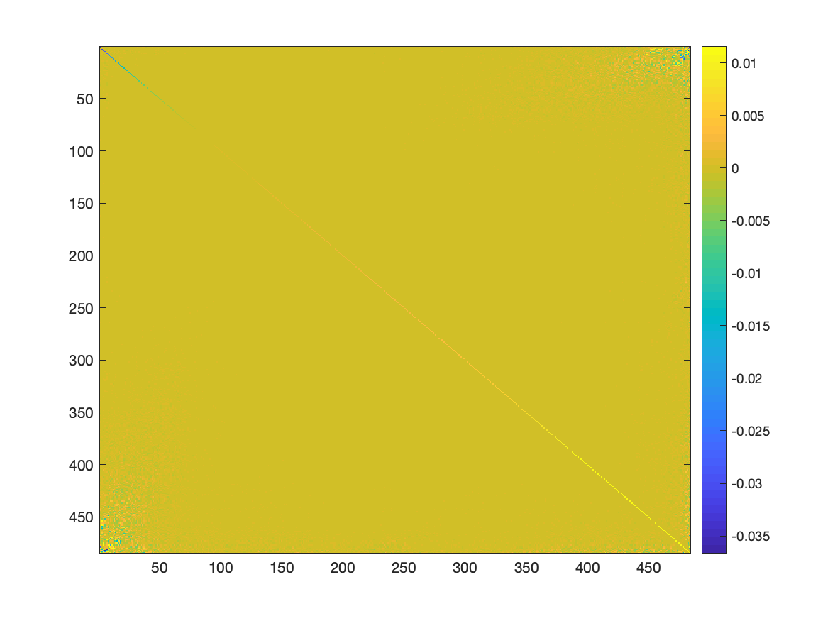
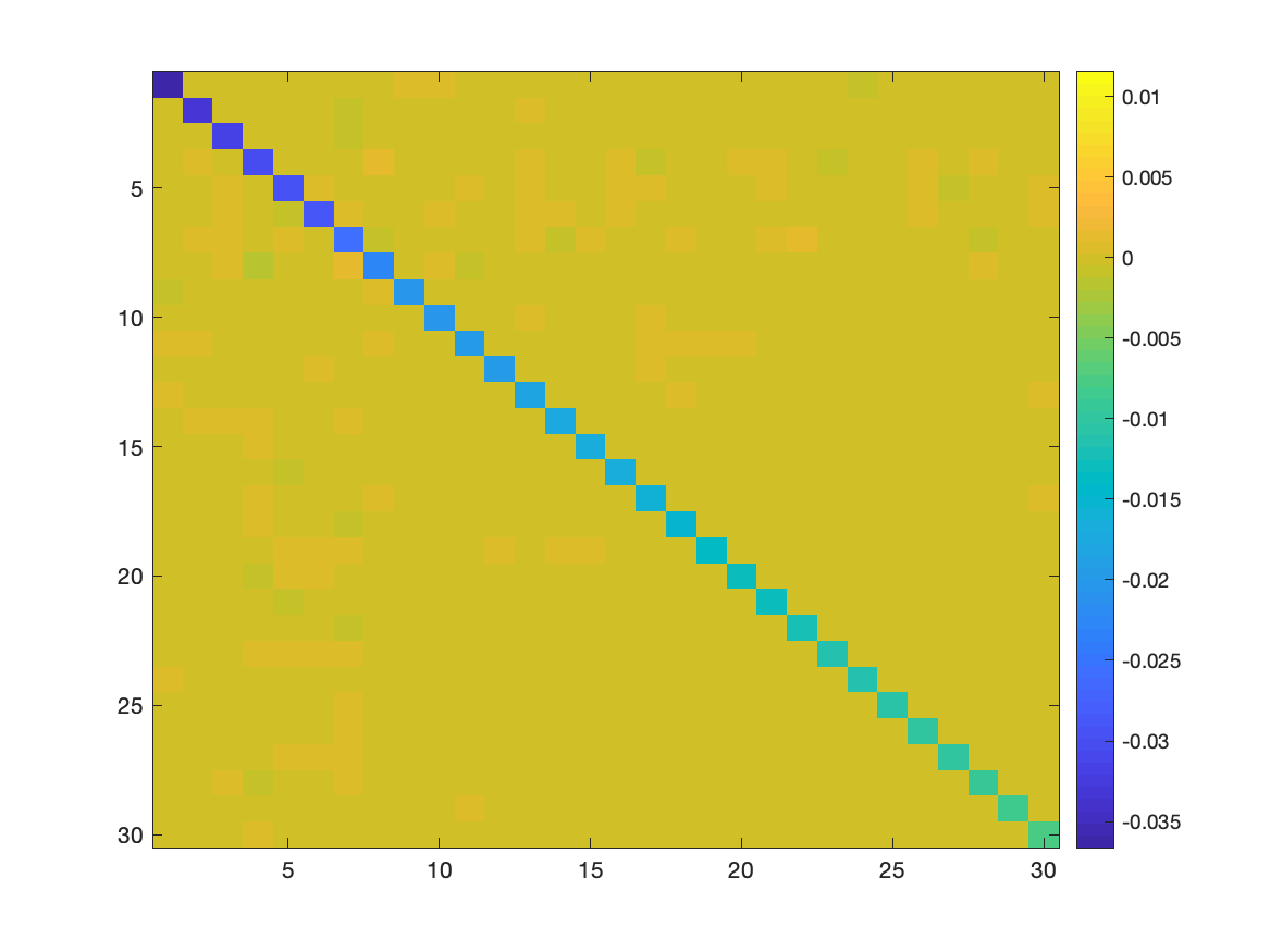
We then randomly pick training input $U\in V_{s}$ such that $U=\sum_{i=1}^{r}c_{i}v_{i}$. The $\mathcal{NN}(\cdot)$ is then trained with $(U,\mathcal{\hat{L}}(U))$-like training pairs, and we obtain a corresponding operator $\mathcal{L}(\cdot)$ with trained coefficients. The linear operators of $\mathcal{L}(\cdot)$ and $\mathcal{\hat{L}}(\cdot)$ are compared by their eigenvalues, i.e. $V^{T}\hat{W}V$ and $V^{T}W^{2}W^{1}V$. By the definition of $V$, the former will exactly be a diagonal matrix with $\lambda_{i}$ be its diagonal value. We expect $W^{2}W^{1}$ functions similarly to $\hat{W}$ on $V_{r}$, and further the $r$-by-$r$ sub-matrix of $V^{T}W^{2}W^{1}V$ should be similar to that of $V^{T}\hat{W}V$.

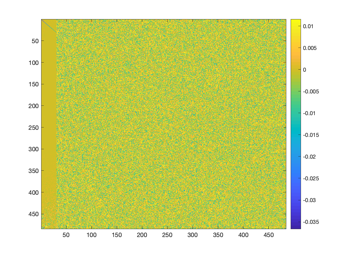
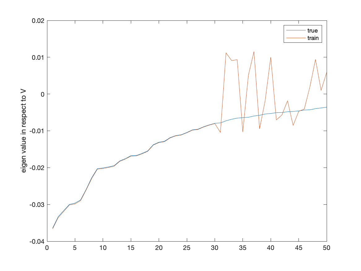
Figure 5 compares $V^{T}W^{2}W^{1}V$ and $V^{T}\hat{W}V$ for the case when $V_{r}$ is constructed letting $r=30$. We can tell that the first $30\times 30$ submatrix are very much alike. That is to say, despite the fact that the operator $\mathcal{L}(\cdot)$ and $\mathcal{\hat{L}}(\cdot)$ are different on $\mathbb{R}^{m}$, their behavior on the subspace $V_{r}$ are the same. Moreover, Figure 6, shows that such similarity only exist in $V_{r}$ as for the $i_{th}$ diagonal values of $V^{T}W^{2}W^{1}V$ and that of $V^{T}\hat{W}V$ distinct when $i>s$. This also makes sense as the operator $\mathcal{L}(\cdot)$ is defined from the trained parameters of $\mathcal{NN}(\cdot)$ where only subspace $V_{r}$ is visible to the network.

(a) $V^{T}\hat{W}V$

(b) $30\times 30$ sub-matrix of $V^{T}\hat{W}V$

(c) $V^{T}W^{2}W^{1}V$

(d) $30\times 30$ sub-matrix of $V^{T}W^{2}W^{1}V$

Figure 5: $\hat{W}$ and $W^{2}W^{1}$ function similarly on $S$, where $r=30$.

Figure 6: Comparison of eigen-values of $\hat{W}$ and $W^{2}W^{1}$ when $r=30$.

5.2 One-layer reduced order neural network

In this example, we consider the one-layer reduced-order neural network as defined in (18). We use this neural network to predict a one-step fluid dynamics, where the data are taken to be NLMC solution coefficients to (1) in the form $(U^{0}_{i},U^{1}_{i})$. We fix $\kappa(t,x)$ and $f(t,x)$ among samples, thus all data describes linear dynamics for different initial conditions.

We take $2\%$ out of all data pairs as testing samples and the remaining $98\%$ as training samples and use only the training sample to train $\mathcal{NN}(\cdot)$. We then evaluate the neural network by examining the accuracy of the following approximation for the unseen testing samples:

$$U^{1}\approx\mathcal{NN}(U^{0}).$$

The $\ell_{2}$ relative error of the prediction is computed by

$$\frac{||U^{1}-\mathcal{NN}(U^{0})||_{2}}{||U^{1}||_{2}}.$$ (44)

Table 1 is the error table for the case when we use $500$ data pairs with $490$ to be training samples and $10$ to be testing samples. These data are generated with different choice of initial condition $U_{i}^{0}$. To match the realistic physical situation, we took all initial conditions to be the NLMC terminal pressure of a mobility driven nonlinear flow process.

Sample Index	Error(%)
#1	0.25
#2	0.43
#3	10.02
#4	9.91
#5	3.90
#6	8.18
#7	17.27
#8	1.57
#9	1.13
#10	0.76
Mean	5.34

Table 1: $\ell_{2}$ relative error of $\mathcal{NN}(\cdot)$ prediction.

From Table 1, we can see that the prediction of our proposed network $\mathcal{NN}(U^{0})$ is rather effective with an average $\ell_{2}$ error of $5.34\%$.

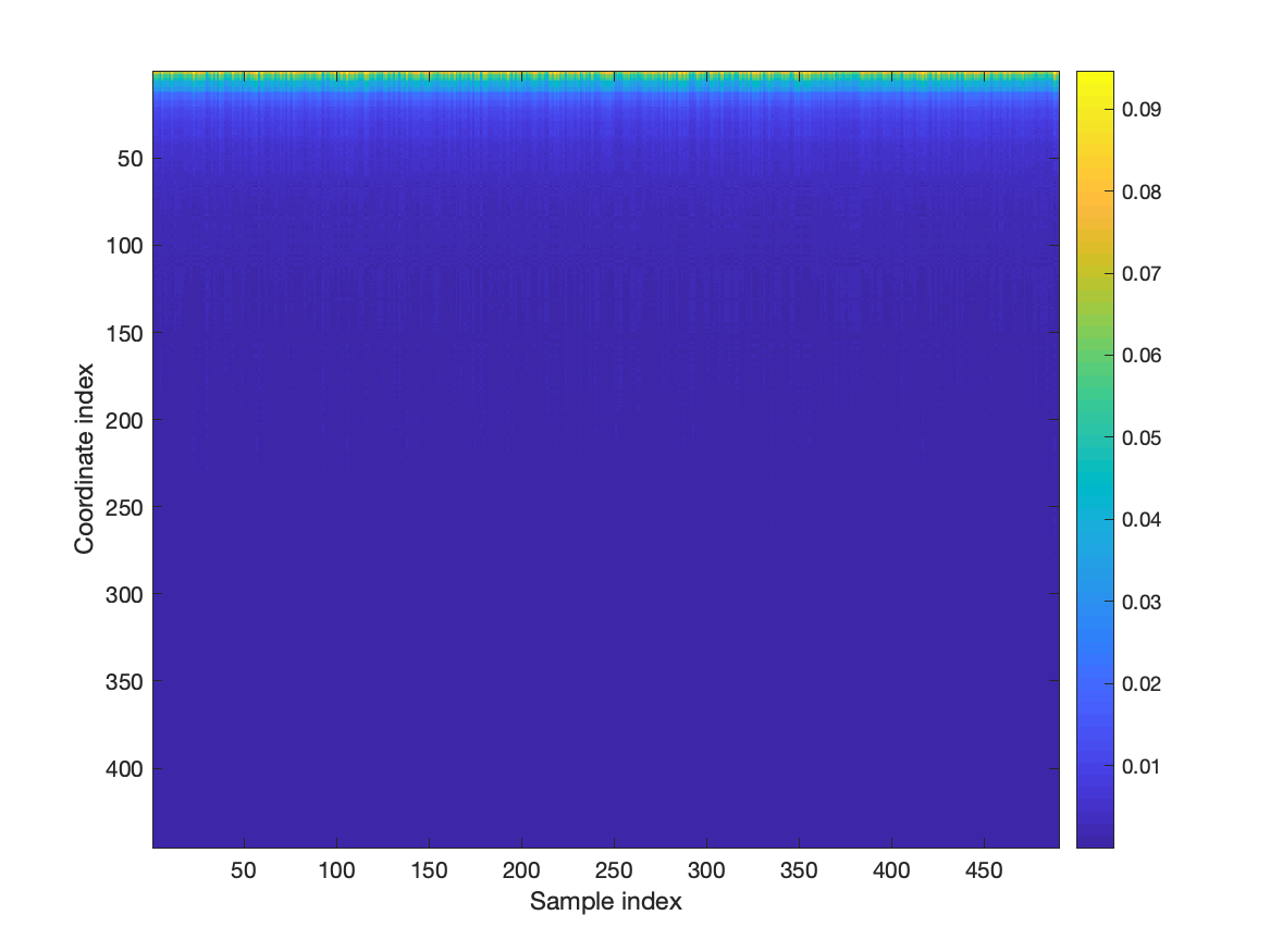
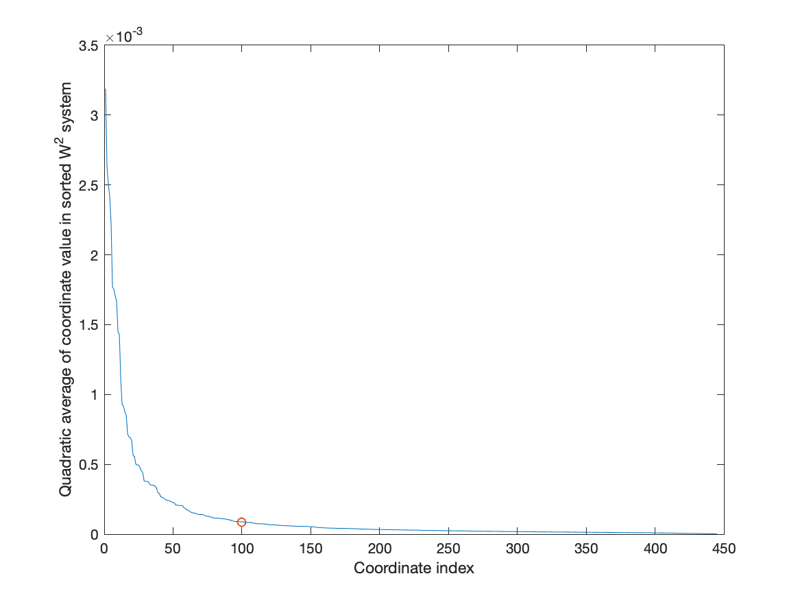
We also verify that $U^{1}$ is sparse in the learned $W^{2}$-system for all data(training and testing). We first reorder the columns of $W^{2}$ by their dominance as discussed in Section 4.3, then compute the corresponding $W^{2}$-system coefficients $U^{1,W^{2}}$, which should be a roughly decreasing vector. From Figure 7, we can tell that the $W^{2}$-system coefficients $U^{1,W^{2}}$ are sparse. This can be an reflection of successful learning of $\hat{W^{2}}$ in Assumption 1. Moreover, only a few dominant modes are needed to recover the solution as the quadratic averages of coordinates $|U^{1,W^{2}}_{j}|$ decays fast when $j>100$.

(a) $U^{1,W^{2}}$ for all data samples

(b) quadratic average of $U^{1,W^{2}}$ among all data samples

Figure 7: Sparsity of the output of $\mathcal{NN}(U^{0})$ in $W^{2}$ .

In a word, the proposed neural network can indeed learn the dominant multiscale modes needed to represent $U^{1}$ from training data while properly reproduce the map between $U^{0}$ and $U^{1}$.

5.3 Model reduction with $W^{2}$

As discussed in Section 4.3, we would like to used the reduced-order system $W^{2,s}$ to further conduct model reduction. The reduced-order solution coefficient is defined with the reduced-order linear operator $\mathcal{L}_{s}(\cdot)$:

$$U^{n+1}_{sN}=\mathcal{L}_{s}(U^{n}).$$ (45)

Noticing that $U^{n+1}_{sN}$ is the coefficient of $u_{h}^{n+1}$ in the original basis system $\{\phi_{j}\}_{j=1}^{m}$ while it is sparse in $W^{2}$-system, i.e, $U^{n+1,W^{2}}_{sN}$ is sparse and has maximum $s$ nonzero elements.

The numerical experiments is conduced based on a one-layer neural network as defined in (18) for a one-step linear dynamics. We would like to compare the following coefficient vectors:

$$U^{1}_{sN}:=\mathcal{L}_{s}(U^{0})=W^{2,s}W^{1}\cdot U^{0}+W^{2,s}b,$$

$$U^{1}_{\text{true}}=\hat{W}U^{0}+\hat{b},$$

and

$$U^{1}_{N}:=\mathcal{NN}(U^{0}).$$

Here $U^{1}_{\text{true}}$ is the true solution to (20), while $U^{1}_{N}$ is the prediction of $\mathcal{NN}(\cdot)$.

Figure 8: Decay of relative error $\frac{||U^{1}_{sN}-U^{1}_{\text{true}}||_{2}}{||U^{1}_{\text{true}}||_{2}}$ as $s$ grows.

	5	10	20	40	80	160	320
#1	66.71	46.80	29.02	17.01	8.44	3.53	1.11
#2	66.55	46.58	29.03	17.41	9.48	4.62	1.59
#3	66.35	46.77	29.70	18.59	12.26	10.92	10.16
#4	67.95	48.58	31.23	19.87	12.59	10.03	9.90
#5	66.22	46.31	28.99	17.73	10.49	6.49	4.34
#6	66.47	46.76	29.40	17.89	10.86	9.12	8.33
#7	69.59	51.33	36.01	27.42	22.33	18.62	17.29
#8	66.60	46.61	28.81	16.39	7.47	3.86	1.96
#9	66.90	47.13	29.21	16.94	8.02	3.58	1.67
#10	67.14	47.39	29.44	17.23	8.23	3.19	1.32
Mean	67.05	47.43	30.08	18.65	11.02	7.40	5.77

Table 2: Decay of error $\frac{||U^{1}_{sN}-U^{1}_{\text{true}}||_{2}}{||U^{1}_{\text{true}}||_{2}}$ with respect to number of selected dominant modes in $W^{2,s}$.

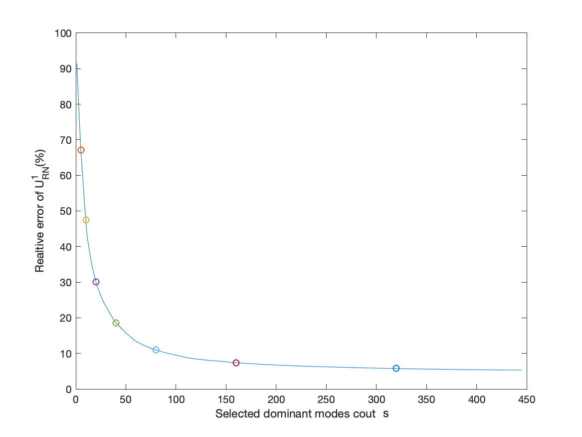
Figure 8 shows the error decay of $U^{1}_{sN}$ compared to $U^{1}_{\text{true}}$. As $s$ grows, the error gets smaller. This figure actually verified (41), i.e. the reduced operator $\mathcal{L}_{s}(\cdot)$ can approximate $\mathcal{\hat{L}}(\cdot)$.Moreover, this approximation gets more accurate as $s$ gets larger. The error in Figure 8 at $s=m=445$ is also expected that it is a consequence of the training error. Besides, we observe that the error decays fast when $s>40$ for our training samples.

Table 2 further facilitates such conclusion. The error of $U^{1}_{sN}$ is less than $12\%$ when $s\geq 80$. We can thus represent the multiscale solution $u_{h}^{1}$ using $s=80$ basis with little sacrifice in the solution accuracy. We notice that the order of the reduce operator $\mathcal{L}_{s}(\cdot)$ is only around $18\%$ that of the original multiscale model.

We lastly present the comparison between $U^{1}_{\text{true}}$, $U^{1}_{N}$, and $U^{1}_{sN}$.From Table 3, we can tell that for a single testing sample, we have

$$\frac{||U^{1}_{sN}-U^{1}_{\text{true}}||_{2}}{||U^{1}_{\text{true}}||_{2}}>\frac{||U^{1}_{N}-U^{1}_{\text{true}}||_{2}}{||U^{1}_{\text{true}}||_{2}},\quad\frac{||U^{1}_{sN}-U^{1}_{\text{true}}||_{2}}{||U^{1}_{\text{true}}||_{2}}>\frac{||U^{1}_{sN}-U^{1}_{N}||_{2}}{||U^{1}_{N}||_{2}},$$

which is as expected since $\frac{||U^{1}_{N}-U^{1}_{\text{true}}||_{2}}{||U^{1}_{\text{true}}||_{2}}$and $\frac{||U^{1}_{sN}-U^{1}_{N}||_{2}}{||U^{1}_{N}||_{2}}$ are exactly the two components of error $\frac{||U^{1}_{sN}-U^{1}_{\text{true}}||_{2}}{||U^{1}_{\text{true}}||_{2}}$. They stands for neural network prediction error and $\mathcal{L}_{s}$ truncation error, respectively. The latter can be reduce by increasing $s$, while the former one can only be improved with more effective training.

Sample Index	$\frac{||U^{1}_{N}-U^{1}_{\text{true}}||_{2}}{||U^{1}_{\text{true}}||_{2}}$	$\frac{||U^{1}_{sN}-U^{1}_{\text{true}}||_{2}}{||U^{1}_{\text{true}}||_{2}}$	$\frac{||U^{1}_{sN}-U^{1}_{N}||_{2}}{||U^{1}_{N}||_{2}}$
#1	0.25	6.48	6.41
#2	0.43	7.65	7.55
#3	10.02	11.59	5.81
#4	9.91	11.28	5.83
#5	3.90	8.93	8.38
#6	8.18	10.00	5.80
#7	17.27	20.98	10.25
#8	1.57	5.85	5.83
#9	1.13	6.13	6.03
#10	0.76	6.17	6.12
Mean	5.34	9.50	6.80

Table 3: Relative error percentage of solutions obtained in full $W^{2}$ system and reduced-order system $W^{2,s}$ for $s=100$.

5.4 Multi-layer reduced order Neural Network

In this example, we use a multi-layer reduced-order neural network $\mathcal{NN}(\cdot)$ to predict multi-step fluid dynamics. Recall (15), it is defined as

$$\mathcal{NN}(\mathbf{x}^{0}):=\mathcal{N}^{n}(\cdots\mathcal{N}^{1}(\mathcal{N}^{0}(\mathbf{x}^{0}))).$$

The input of $\mathcal{NN}(\cdot)$ is taken to be $U^{0}$, the initial condition, while the outputs are the collection of outputs at $n_{th}$-layer sub-network $\mathcal{N}^{n}(\cdot)$ which correspond to the true values [$U^{1},U^{2},\cdots,U^{9}$]. $U^{n+1}$ are all taken to be NLMC solutions of (1) at time step $n$ for $n=0,\cdots,8$. Prediction accuracy is measured with $\ell_{2}$ relative error that defined similar to (44).

Sample Index	$U^{1}$	$U^{2}$	$U^{3}$	$U^{4}$	$U^{5}$	$U^{6}$	$U^{7}$	$U^{8}$	$U^{9}$
#1	1.62	1.17	1.69	1.91	1.95	1.92	1.92	1.91	1.96
#2	3.33	1.86	2.10	1.98	2.15	1.53	1.04	0.94	0.77
#3	11.62	13.32	9.39	9.57	8.89	10.36	11.67	11.86	12.97
#4	9.74	9.00	4.21	3.45	3.46	3.17	2.93	2.87	2.81
#5	5.63	4.68	2.65	2.28	2.52	1.89	1.49	1.74	1.91
#6	9.54	11.50	9.30	9.70	9.14	10.50	11.73	12.00	13.09
#7	21.46	14.82	5.42	4.24	3.27	5.06	6.52	6.77	7.81
#8	5.72	1.40	0.67	0.77	1.11	1.49	1.95	2.54	3.20
#9	4.03	2.16	3.21	3.66	3.47	4.36	5.15	5.35	5.97
#10	4.62	1.01	3.14	3.84	3.81	4.47	5.05	5.24	5.68
Mean	7.73	6.09	4.18	4.14	3.98	4.47	4.95	5.12	5.62

Table 4: $\ell_{2}$ relative error of prediction of $U^{n+1}$ using $\mathcal{NN}(\cdot)$.

In Table 4, the columns shows the prediction error for $U^{n+1},n=0,1,\cdots 8$ where the average error is computed for all time steps among testing samples which are less than $10\%$ in average. Therefore, we claim that the proposed multi-layer reduced order neural network $\mathcal{NN}(\cdot)$ is effective in the aspect of prediction. We also claim that the coefficient $U^{n+1,W_{n}^{2}}$ for $n=0,1,\cdots,8$ are sparse in the independent systems $W^{2}_{n}$. These systems are again learned simultaneously by training $\mathcal{NN}(\cdot)$.

5.5 Clustering

In this experiment, we aim to model the fluid dynamics correspond to two different fractured media as shown in Figure 9. More specifically, the permeability coefficient of matrix region have $\kappa_{m}=1$ and the permeability of the fractures are $\kappa_{f}=10^{3}$. The one-step NLMC solutions pairs $(U^{0},U^{1})$ are generated following these two different configurations of fracture are then referred as “Cluster 1” and “Cluster 2” (see Figure 10 for an illustration). We will then compare the one-step prediction of networks $\mathcal{NN}_{1},\mathcal{NN}_{2}$ with that of $\mathcal{NN}_{\text{mixed}}$. The input are taken taken to be $U^{0}$, which are chosen to be the terminal solution of mobility driven 10-step nonlinear dynamics, while the output is an approximation of $U^{1}$.

$\mathcal{NN}_{1},\mathcal{NN}_{2}$ and $\mathcal{NN}_{\text{mixed}}$ share same one-layer soft thresholding neural network structure as in (18) while the first two network are trained with data for each cluster separately and the latter one is trained with mixed data for two clusters.

(a) Cluster 1

(b) Cluster 2

Figure 9: Fracture networks for two clusters.

(a) Coarse-scale NLMC solution $u^{0}$ – Cluster 1

(b) Coarse-scale solution of pressure $u^{0}$ – Cluster 2

(c) Coarse-scale solution of pressure $u^{1}$ – Cluster 1

(d) Coarse-scale solution of pressure $u^{1}$ – Cluster 2

Figure 10: Example solution pairs for two different clusters.

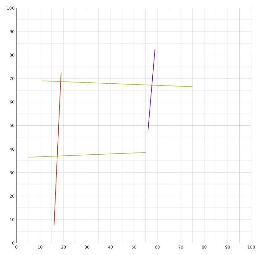
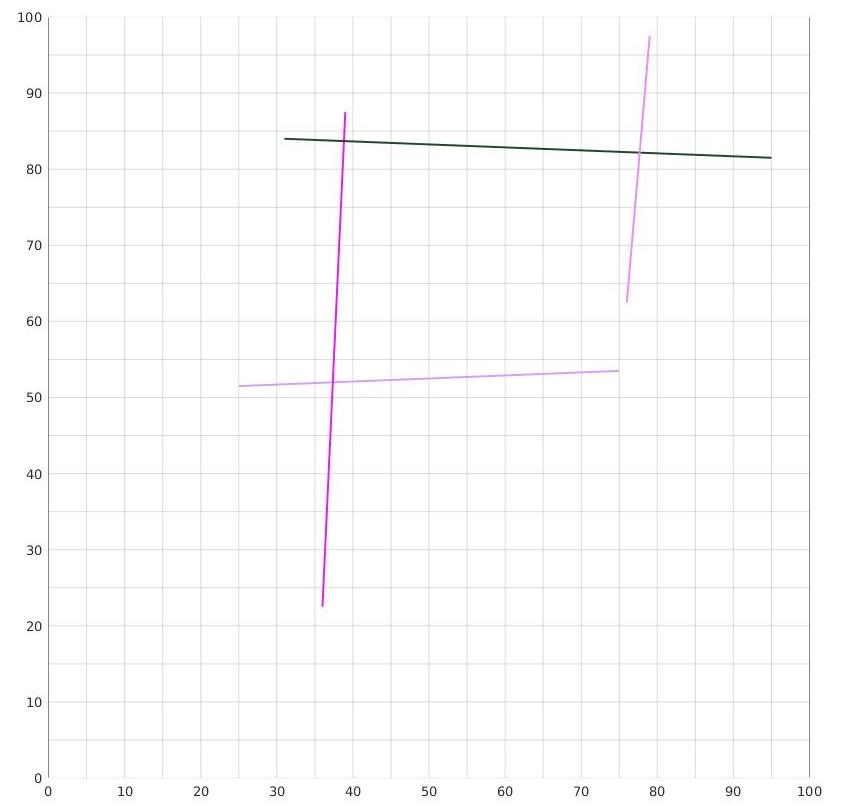
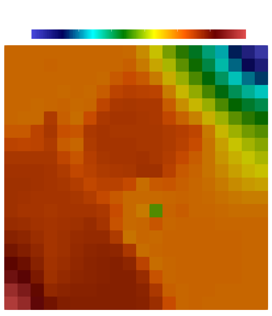
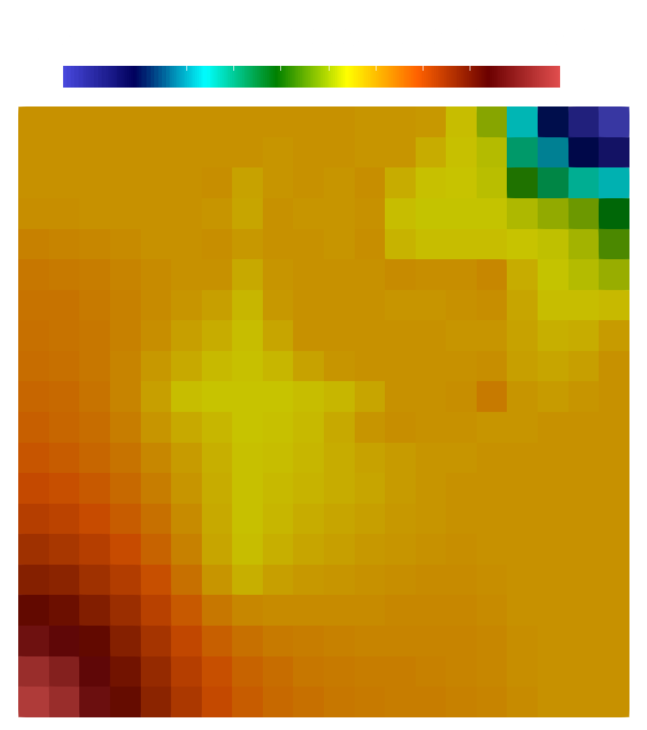
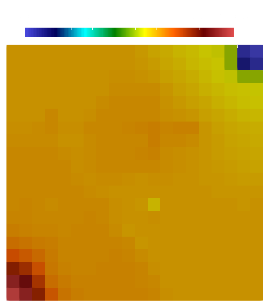
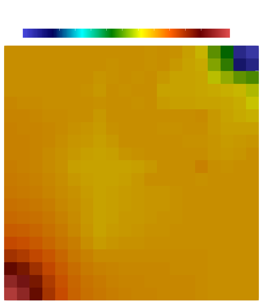
Figure 9 shows the fracture network we use to generate data for two clusters, while Figure 10 shows an example of solution $U^{0}$ and $U^{1}$ for each cluster. As observed from the profiles of $U^{0}$ and $U^{1}$, we can see that these the solutions are very different due to the translation of the fractures. Moreover, since the data resulted from both clusters have non-uniform map between $U^{0}$ and $U^{1}$, the mixed data set can be considered as obtained from a nonlinear map.

Sample Index	Cluster 1 Error	Cluster 2 Error
#1	0.87	0.26
#2	3.19	0.45
#3	13.62	0.79
#4	12.36	0.49
#5	7.64	0.43
#6	10.69	1.00
#7	19.08	0.53
#8	2.57	0.92
#9	0.77	0.46
#10	3.70	0.38
Mean	7.45	0.57

(a) Relative $\ell_{2}$ prediction error(%) of $\mathcal{N}_{1}$ and $\mathcal{N}_{2}$.

Sample Index	Cluster 1 Error	Cluster 2 Error
# 1	36.25	84.83
#2	35.08	84.20
#3	28.20	111.05
#4	44.60	69.35
#5	32.32	89.30
#6	30.03	106.41
#7	48.61	57.76
#8	35.63	88.46
#9	36.89	88.67
#10	38.78	83.85
Mean	36.64	86.39

(b) Relative $\ell_{2}$ prediction error(%) of $\mathcal{N}_{\text{mixed}}$.

Table 5: Prediction error of $\mathcal{N}_{1}$, $\mathcal{N}_{2}$ and $\mathcal{N}_{\text{mixed}}$.

Table 5 demonstrates the comparison of the prediction accuracy when the network is fed with a single cluster data and when the network is fed with a mixed data. This simple treatment can significantly improve the accuracy. For Cluster 1, the average prediction error of $\mathcal{NN}_{1}$ is around $7.45\%$ while that of the $\mathcal{NN}_{\text{mixed}}$ is around $36.64\%$. Similar contrast can also be observed for Cluster 2.

6 Conclusion

In this paper, we discuss a novel deep neural network approach to model reduction approach for multiscale problems. To numerically solve multiscale problems, a fine grid needs to be used and results in a huge number of degrees of freedom. To this end, non-local multicontinuum (NLMC) upscaling [18] is used as a dimensionality reduction technique. In flow dynamics problems, multiscale solutions at consecutive time instants are regarded as an input-output mechanism and learnt from deep neural networks techniques. By exploiting a relation between a soft-thresholding neural network and $\ell_{1}$ minimization, multiscale features of the coarse-grid solutions are extracted using neural networks. This results in a new neural-network-based construction of reduced-order model, which involves extracting appropriate important modes at each time step. We also suggest an efficient strategy for a class of nonlinear flow problems. Finally, we present numerical examples to demonstrate the performance of our method applied to some selected problems.

References

- [1] Martín Abadi, Ashish Agarwal, Paul Barham, Eugene Brevdo, Zhifeng Chen, Craig Citro, Greg S. Corrado, Andy Davis, Jeffrey Dean, Matthieu Devin, Sanjay Ghemawat, Ian Goodfellow, Andrew Harp, Geoffrey Irving, Michael Isard, Yangqing Jia, Rafal Jozefowicz, Lukasz Kaiser, Manjunath Kudlur, Josh Levenberg, Dandelion Mané, Rajat Monga, Sherry Moore, Derek Murray, Chris Olah, Mike Schuster, Jonathon Shlens, Benoit Steiner, Ilya Sutskever, Kunal Talwar, Paul Tucker, Vincent Vanhoucke, Vijay Vasudevan, Fernanda Viégas, Oriol Vinyals, Pete Warden, Martin Wattenberg, Martin Wicke, Yuan Yu, and Xiaoqiang Zheng. TensorFlow: Large-scale machine learning on heterogeneous systems, 2015. Software available from tensorflow.org.
- [2] Assyr Abdulle and Yun Bai. Adaptive reduced basis finite element heterogeneous multiscale method. Comput. Methods Appl. Mech. Engrg., 257:203–220, 2013.
- [3] G. Allaire and R. Brizzi. A multiscale finite element method for numerical homogenization. SIAM J. Multiscale Modeling and Simulation, 4(3):790–812, 2005.
- [4] Manal Alotaibi, Victor M. Calo, Yalchin Efendiev, Juan Galvis, and Mehdi Ghommem. Global–local nonlinear model reduction for flows in heterogeneous porous media. Computer Methods in Applied Mechanics and Engineering, 292:122–137, 2015.
- [5] T. Arbogast. Implementation of a locally conservative numerical subgrid upscaling scheme for two-phase Darcy flow. Comput. Geosci, 6:453–481, 2002.
- [6] Amir Beck and Marc Teboulle. A fast iterative shrinkage-thresholding algorithm for linear inverse problems. SIAM journal on imaging sciences, 2(1):183–202, 2009.
- [7] I. Bilionis and N. Zabaras. Solution of inverse problems with limited forward solver evaluations: a bayesian perspective. Inverse Problems, 30(015004), 2013.
- [8] Ilias Bilionis, Nicholas Zabaras, Bledar A. Konomi, and Guang Lin. Multi-output separable gaussian process: Towards an efficient, fully bayesian paradigm for uncertainty quantification. Journal of Computational Physics, 241:212–239, 2013.
- [9] Hervé Bourlard and Yves Kamp. Auto-association by multilayer perceptrons and singular value decomposition. Biological cybernetics, 59(4-5):291–294, 1988.
- [10] Donald L Brown and Daniel Peterseim. A multiscale method for porous microstructures. arXiv preprint arXiv:1411.1944, 2014.
- [11] E. Chung, Y. Efendiev, and S. Fu. Generalized multiscale finite element method for elasticity equations. International Journal on Geomathematics, 5(2):225–254, 2014.
- [12] E. Chung, Y. Efendiev, and W. T. Leung. Generalized multiscale finite element method for wave propagation in heterogeneous media. SIAM Multicale Model. Simul., 12:1691–1721, 2014.
- [13] E. Chung and W. T. Leung. A sub-grid structure enhanced discontinuous galerkin method for multiscale diffusion and convection-diffusion problems. Communications in Computational Physics, 14:370–392, 2013.
- [14] E. T. Chung, Y. Efendiev, W.T. Leung, M. Vasilyeva, and Y. Wang. Online adaptive local multiscale model reduction for heterogeneous problems in perforated domains. Applicable Analysis, 96(12):2002–2031, 2017.
- [15] E. T. Chung, Y. Efendiev, and G. Li. An adaptive GMsFEM for high contrast flow problems. J. Comput. Phys., 273:54–76, 2014.
- [16] Eric Chung, Yalchin Efendiev, and Thomas Y Hou. Adaptive multiscale model reduction with generalized multiscale finite element methods. Journal of Computational Physics, 320:69–95, 2016.
- [17] Eric Chung, Maria Vasilyeva, and Yating Wang. A conservative local multiscale model reduction technique for stokes flows in heterogeneous perforated domains. Journal of Computational and Applied Mathematics, 321:389–405, 2017.
- [18] Eric T Chung, Efendiev, Wing Tat Leung, Maria Vasilyeva, and Yating Wang. Non-local multi-continua upscaling for flows in heterogeneous fractured media. arXiv preprint arXiv:1708.08379, 2018.
- [19] Eric T Chung, Yalchin Efendiev, Wing Tat Leung, Maria Vasilyeva, and Yating Wang. Non-local multi-continua upscaling for flows in heterogeneous fractured media. Journal of Computational Physics, 2018.
- [20] Martin Drohmann, Bernard Haasdonk, and Mario Ohlberger. Reduced basis approximation for nonlinear parametrized evolution equations based on empirical operator interpolation. SIAM J. Sci. Comput., 34(2):A937–A969, 2012.
- [21] W. E and B. Engquist. Heterogeneous multiscale methods. Comm. Math. Sci., 1(1):87–132, 2003.
- [22] Y. Efendiev, J. Galvis, and E. Gildin. Local-global multiscale model reduction for flows in highly heterogeneous media. Submitted.
- [23] Y. Efendiev, J. Galvis, and T. Y. Hou. Generalized multiscale finite element methods (gmsfem). Journal of Computational Physics, 251:116–135, 2013.
- [24] Y. Efendiev, J. Galvis, and X.H. Wu. Multiscale finite element methods for high-contrast problems using local spectral basis functions. Journal of Computational Physics, 230:937–955, 2011.
- [25] Yalchin Efendiev, Juan Galvis, and Thomas Y Hou. Generalized multiscale finite element methods (gmsfem). Journal of Computational Physics, 251:116–135, 2013.
- [26] Jacob Fish and Wen Chen. Space–time multiscale model for wave propagation in heterogeneous media. Computer Methods in applied mechanics and engineering, 193(45):4837–4856, 2004.
- [27] Jacob Fish and Rong Fan. Mathematical homogenization of nonperiodic heterogeneous media subjected to large deformation transient loading. International Journal for numerical methods in engineering, 76(7):1044–1064, 2008.
- [28] M. Ghommem, M. Presho, V. M. Calo, and Y. Efendiev. Mode decomposition methods for flows in high-contrast porous media. global-local approach. Journal of Computational Physics, 253:226–238.
- [29] Patrick Henning and Mario Ohlberger. The heterogeneous multiscale finite element method for elliptic homogenization problems in perforated domains. Numerische Mathematik, 113(4):601–629, 2009.
- [30] Diederik P Kingma and Jimmy Ba. Adam: A method for stochastic optimization. arXiv preprint arXiv:1412.6980, 2014.
- [31] X. Ma, M. Al-Harbi, A. Datta-Gupta, and Y. Efendiev. A multistage sampling approach to quantifying uncertainty during history matching geological models. SPE Journal, 13(10):77–87, 2008.
- [32] Ana-Maria Matache and Christoph Schwab. Two-scale fem for homogenization problems. ESAIM: Mathematical Modelling and Numerical Analysis, 36(04):537–572, 2002.
- [33] A. Mondal, Y. Efendiev, B. Mallick, and A. Datta-Gupta. Bayesian uncertainty quantification for flows in heterogeneous porous media using reversible jump Markov Chain Monte-Carlo methods. Adv. Water Resour., 33(3):241–256, 2010.
- [34] H. Owhadi and L. Zhang. Metric-based upscaling. Comm. Pure. Appl. Math., 60:675–723, 2007.
- [35] Prajit Ramachandran, Barret Zoph, and Quoc V Le. Searching for activation functions. 2018.
- [36] Jürgen Schmidhuber. Deep learning in neural networks: An overview. Neural networks, 61:85–117, 2015.
- [37] Yating Wang, Siu Wun Cheung, Eric T. Chung, Yalchin Efendiev, and Min Wang. Deep multiscale model learning. arXiv preprint arXiv:1806.04830, 2018.
- [38] Yanfang Yang, Mohammadreza Ghasemi, Eduardo Gildin, Yalchin Efendiev, Victor Calo, et al. Fast multiscale reservoir simulations with pod-deim model reduction. SPE Journal, 21(06):2–141, 2016.
- [39] Yinhao Zhu and Nicholas Zabaras. Bayesian deep convolutional encoder–decoder networks for surrogate modeling and uncertainty quantification. Journal of Computational Physics, 366:415–447, 2018.