Physical Foundations of Landauer’s Principle

Abstract

We review the physical foundations of Landauer’s Principle, which relates the loss of information from a computational process to an increase in thermodynamic entropy. Despite the long history of the Principle, its fundamental rationale and proper interpretation remain frequently misunderstood. Contrary to some misinterpretations of the Principle, the mere transfer of entropy between computational and non-computational subsystems can occur in a thermodynamically reversible way without increasing total entropy. However, Landauer’s Principle is not about general entropy transfers; rather, it more specifically concerns the ejection of (all or part of) some correlated information from a controlled, digital form (e.g., a computed bit) to an uncontrolled, non-computational form, i.e., as part of a thermal environment. Any uncontrolled thermal system will, by definition, continually re-randomize the physical information in its thermal state, from our perspective as observers who cannot predict the exact dynamical evolution of the microstates of such environments. Thus, any correlations involving information that is ejected into and subsequently thermalized by the environment will be lost from our perspective, resulting directly in an irreversible increase in total entropy. Avoiding the ejection and thermalization of correlated computational information motivates the reversible computing paradigm, although the requirements for computations to be thermodynamically reversible are less restrictive than frequently described, particularly in the case of stochastic computational operations. There are interesting possibilities for the design of computational processes that utilize stochastic, many-to-one computational operations while nevertheless avoiding net entropy increase that remain to be fully explored.

1 Introduction

A core motivation for the field of reversible computation is Landauer’s Principle [1], which tells us that each bit’s worth of information that is lost from a computational process results in a (permanent) increase in thermodynamic entropy of $\mathrm{\Delta}S\geq k\ln 2$, where $k=k_{\mathrm{B}}$ is Boltzmann’s constant, with the corresponding dissipation of $\mathrm{\Delta}E\geq kT\ln 2$ energy to heat, where $T$ is the temperature of the heat sink. By avoiding information loss, reversible computation bypasses this limit on the energy efficiency of computing, opening the door to a future of potentially unlimited long-term improvements in computational efficiency.

The correctness of Landauer’s Principle has recently been empirically validated [5, 6, 7, 8], but the results of these experiments are unsurprising, given that the validity of Landauer’s Principle can be shown to follow as a rigorous consequence of basic facts of fundamental physics that have been known for over a century, ever since pioneering work by such luminaries as Boltzmann and Planck revealed the fundamentally statistical nature of entropy, summarized in the equation $S=k\log W$ that is emblazoned on Boltzmann’s tombstone. As we will show in some detail, Landauer’s Principle follows directly and rigorously from the modern statistical-mechanical understanding of thermodynamics (which elaborates upon Boltzmann’s view), augmented only by a few mathematical concepts from information theory, along with the most basic understanding of what is meant by a computational process.

However, despite this underlying simplicity, certain subtleties regarding the proper interpretation of the Principle remain frequently misunderstood; I have discussed some of these in earlier papers [9, 10, 11, 12, 13], and will elaborate upon another one in the present paper. Issues mentioned in these works include:

1. Treatment of stochastic operations. It has long been understood that stochastic or randomizing computational operations can transfer entropy from a thermodynamic environment to a digital form, reversing the usual process considered in discussions of Landauer, in which computational entropy is pushed from a digital form out to a thermal environment. It follows from this observation that the act of merely transferring isolated bits of entropy between computational and thermal forms can actually be a thermodynamically (albeit not logically) reversible process. As an illustration of this, I pointed out in 2005 [9] that a stochastic computational process that simply re-randomizes an already-random digital bit does not necessarily increase thermodynamic entropy, even though this process would not be considered logically reversible (injective) in a traditional treatment. Thus, the usual arguments for Landauer’s Principle and reversible computing that do not address this case are overly simplistic; later, we will discuss how to generalize and repair them.

2. Transformations of complex states. The fundamental physical arguments behind Landauer’s Principle are not constrained to dealing only with bits (binary digits or two-state systems) per se; they apply equally well to systems with any number of states. In particular, one can even apply them to spatially-extended physical systems with very large numbers of states, so that, for example, it is possible in principle to adiabatically transform a system representing the state of a complex Boolean logic circuit directly from “old state” to “new state” in a single step without incurring any Landauer losses related to the number of Boolean logic operations implemented by the circuit. An abstract model illustrating this capability in the context of classical, chaotic dynamical systems was described in 2016 [10, 14]. An example of an adiabatic physical mechanism that can transform states of extended logic networks all at once can be found in the Quantum-dot Cellular Automata (QDCA or QCA) approach pioneered by Lent et al. (see [15] and subsequent papers by that group). However, an analogous approach can also be carried out even in more conventional CMOS technology, by encoding complex logic functions as large series/parallel switching circuits that are transformed adiabatically in a single (albeit very slow) step.

3. Role of conditional reversibility. A third important clarification of Landauer’s Principle can be found when considering the role of conditional reversibility, which I explained in [9, 11, 12, 13], but which was already implicitly leveraged by all of the early implementation concepts for reversible computation [16, 17, 18, 19]. The key point is that states that are prevented from arising by design within a given computer architecture (construed generally) have zero probability of occurring, and therefore make zero contribution to the entropy that is required to be ejected from the computational state by Landauer’s Principle. Therefore, it is a sufficient logical-level condition for avoiding Landauer’s limit if only the set of computational states that are actually allowed to occur in the context of a given design are mapped one-to-one onto new states. I.e., the machine can be designed in such a way that it would map the other, forbidden states many-to-one without there being any actual thermodynamic impact from this, given that those states will never actually occur. This issue was already discussed extensively in [11] (and see [12] for proofs of the theorems), so we will not discuss it in great detail in the present paper.

4. Importance of correlations. At first, it might seem that the thermodynamic reversibility of certain logically-irreversible, stochastic transformations as discussed in point 1 above contradicts Landauer’s Principle. But this apparent contradiction is resolved when one realizes that the proper subject of Landauer’s Principle is not in fact the ejection of isolated, purely random bits of digital information from a computer. Such bits are already entropy, and merely moving those bits from a stable digital form to a rapidly-changing thermal form does not necessarily increase total entropy, as we will illustrate with some basic examples. Rather, what Landauer’s Principle really concerns is the ejection of correlated bits from the computational state, since a thermal environment cannot be expected to preserve those correlations in any way that is accessible to human modeling. So really, it is the loss of prior correlations that is the ultimate basis for the consideration of information loss and entropy increase in Landauer’s Principle. I addressed this issue briefly in previous presentations [20, 21]; in this paper, I elaborate on it in more detail.

The rest of this paper is organized as follows. Section 2 reviews some basic mathematical concepts of entropy, information, and computation. Section 3 discusses the connection of these concepts with physics in detail, and gives examples of physical systems that illustrate the fundamental appropriateness of these abstract concepts for modeling the practical physical circumstances that we use them to describe. This discussion lays bare the fundamental unity between information theory and physical theory, in showing that information-theoretic entropy and thermodynamic entropy really are the exact same concept as each other; they are, in fact, the exact same epistemological/physical quantity, merely applied at different levels that are nonetheless fundamentally interconnected. We then use this understanding of basic physics to prove Landauer’s Principle, and discuss its implications for the energy efficiency of future reversible and irreversible computing technologies. Section 4 briefly reviews some of the existing laboratory studies that have validated Landauer’s Principle empirically. Section 5 concludes with some suggestions for future work.

2 Definitions of Basic Concepts

In this section, we begin by reviewing the mathematical definitions of some basic concepts from statistics, information theory, and computation that are useful for understanding the thermodynamics of computation in general, and Landauer’s Principle in particular. Later (in sec. 3), we’ll discuss in detail why these mathematical concepts are appropriate not just in abstract conceptual scenarios, but also for describing real physical circumstances, and give some examples.

2.1 Some Basic Statistical Concepts

First, let us define a few basic statistical concepts that are adequate for our purposes. In the following treatment, we will take a manifestly epistemological perspective, since, as we will see, such a perspective is inevitably quite central and fundamental to what not only statistics, but also physical modeling in general is all about—since, any physical model inevitably concerns what is known, or could be known, about a physical system; and this remains the case whether we are talking about the actual knowledge of a real observer (e.g., a human experimentalist), or about what could in principle be known by a hypothetical omniscient modeler, or by any other real or imagined reasoner (e.g., an engineered artifact, considered as an observer). All sciences are concerned with the knowable truths in their domain of applicability, and physics, in particular, is ultimately simply the study of what is knowable about the bottom-most foundations of this physical world that we live in. Thus a proper mathematical account of epistemology is an essential conceptual foundation for any science, and the study of the thermodynamics of computation is no exception.

In the following, we begin with the concept of a discrete variable—where “variable” here is meant in the sense of a random variable in statistics, although we avoid that particular terminology, since it begs the question of defining randomness, which is somewhat tangential to our purposes. Then we go on to motivate and define some basic concepts of improbability, surprise, and probability, along with a concept that we will think of as the “psychological weight” or heaviness of a possible outcome, together with the expected value of a function, and finally entropy (a concept that falls out naturally from the foregoing ones). This means of deriving the entropy concept provides certain conceptual elements that we will find useful in later discussions. (But, we should emphasize that one does not have to take seriously any particular theory of psychology to find these concepts useful—they are simply technical definitions.)

2.1.1 Discrete variables.

To begin, a discrete variable $V$ is associated with some countable set $\mathbf{V}=\{v_{i}\}$ of mutually exclusive values $v_{1},\,v_{2},\,\ldots\in\mathbf{V}$ that the variable can take on. For our purposes, typically we will work with value sets $\mathbf{V}$ that are finite. Our subject matter, in statistics and information theory, is the quantitative analysis of what is known about the value of some variable(s). As usual, the knower, here, could in general be any real or hypothetical reasoner.

2.1.2 Improbability and probability.

Suppose all that is initially known regarding a given discrete variable $V$ is the cardinality (number of elements) $n=|\mathbf{V}|$ of its set $\mathbf{V}$ of possible values. Assume $n$ is finite; we write $\mathbf{V}=\{v_{1},\,v_{2},\,\ldots,\,v_{n}\}$. Now suppose we somehow subsequently learn that the variable has a particular value, $V=v_{i}$, for some $i\in\{1,\,2,\,\ldots,\,n\}$. We can say that this particular outcome or event (of the learned value turning out to be $v_{i}$) has, a priori, from the learner’s perspective, a baseline improbability $m=m_{i}=m(v_{i})$ given by $m_{i}=\overline{m}=n$, since the more different values $v_{i}$ there are, the more unlikely or improbable each individual value would seem to be, proportionally—not knowing anything else about the situation. We can then define the baseline probability $p=p_{i}=p(v_{i})=\overline{p}$ of each value as the reciprocal of its improbability $m=\overline{m}$, i.e., $p_{i}=1/m_{i}=1/n$; note that this derivation yields the usual property that the probabilities of all the values $\{v_{i}\}$ sum to 1, i.e., $\sum_{i=1}^{n}p_{i}=1$.

2.1.3 Surprise, or increase of knowledge.

We can then quantify the amount of increase in our knowledge resulting from this learning event as our surprise, or the surprisingness of the event, defined as $s=s_{i}=s(v_{i})=\log m_{i}=\log 1/p_{i}=-\log p_{i}$ (dimensioned in general logarithmic units; see [22]), with the motivation for this definition being that “surprise” should combine additively whenever the number of possible values combines multiplicatively.

For example, when rolling a 6-sided die, each outcome has an improbability $m$ of 6, and the surprise for each case (rolling a 1, say) is then $s=\log 6.$ If I roll the die twice, there are $6^{2}=36$ possible sequences of outcomes, but each of these sequences (say rolling two 1’s) is, intuitively, only twice as surprising ($\log 36=2\log 6$) as each individual result was in the 1-die case. In any event, regardless of whether the behavior of this definition matches your personal intuition about how surprisingness ought to work, psychologically, let this be our technical definition of “surprise.”

2.1.4 Nonuniform probability distributions.

If we happen to have more knowledge about the value of the variable than just its cardinality, this can be modeled by assigning different probabilities $p_{i}$ (and corresponding improbability and surprise) to different values $v_{i}$, subject to the constraint that the probabilities of all the values are still non-negative, and still sum to 1. We call the entire function $P:\mathbf{V}\rightarrow[0,1]$ with $P(v_{i})=p_{i}$ (over all $i=1,\,2,\,\ldots,\,n$) a probability distribution over $V$, and write it as $P(V)$. In this case, the improbabilities $m_{i}=1/p_{i}$ and surprisingnesses $s_{i}=\log m_{i}$ would be adjusted accordingly.

The semantic interpretation of probabilities in this general case can be inherited from the “surprise” concept; for example, if a particular value $v_{i}$ has probability 1/2, this would mean that its surprise is log 2, and this says that our state of knowledge about the variable is such that, if we were to learn that it had the value $v_{i}$, we would be equally surprised as we would have been if initially we only knew that it had exactly two possible values, and then we suddenly learned that its actual value was one of those. Thus, this way of motivating the concept of probability rests on an intuitive psychological interpretation.

2.1.5 Heaviness, or “psychological weight.”

Next, let’s introduce a new technical concept that we call the heaviness $h(v_{i})$ of a value $v_{i}$, defined as its surprise $s_{i}=s(v_{i})$, weighted by its probability $p_{i}=p(v_{i})$ of occurring:

$$h=h_{i}=h(v_{i})=h(p_{i})=p_{i}\cdot s_{i}=p_{i}\log m_{i}=-p_{i}\log p_{i}.$$ (1)

The heaviness function is plotted in Fig. 1(b). Our use of the word “heaviness” for this concept is intended to evoke an intuitive psychological sense of the word, as in, how heavily does the possibility of this particular outcome weigh on one’s mind? The intuition here is that an extremely unlikely possibility doesn’t (or shouldn’t) weigh on our minds very heavily, and neither should an extremely likely one (since it is a foregone conclusion). This psychological interpretation of the concept will not be important to our later conclusions, though; it is merely provided to aid understanding.

Figure 1: Surprise and heaviness functions. (a) Plot of surprise $s$ (in units of $k=\log\mathrm{e}$) as a function of probability $p$. Note that heaviness $h=ps$ is given by the area of a rectangle drawn between the origin and a point on this curve—if we imagine that the rectangle were a flat sheet of physical material of uniform density and thickness, then its physical heaviness would indeed be proportional to its area. (b) Plot of heaviness (in $k$) as a function of probability. Note that the maximum heaviness of $k/\mathrm{e}$ is associated with events of improbability e.

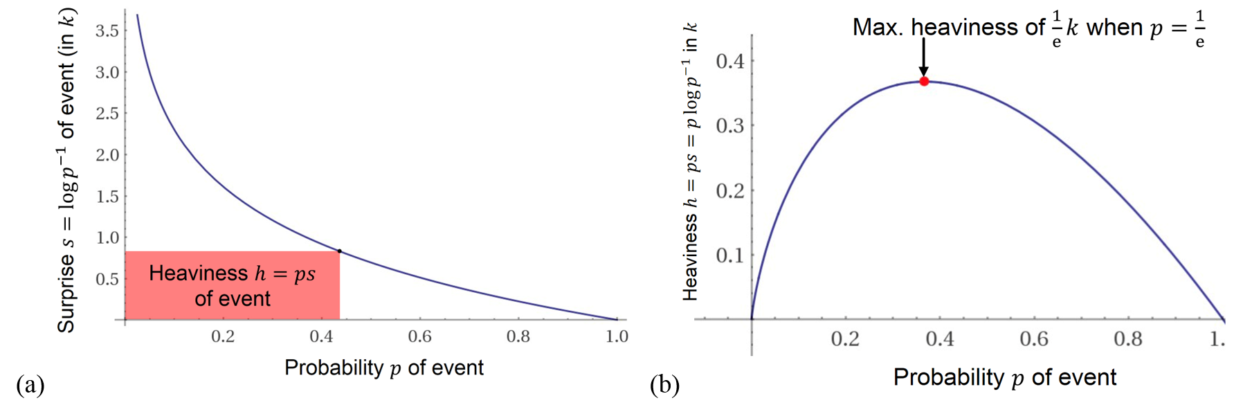
It turns out that with the foregoing definition, the maximum heaviness inheres in an outcome that has an improbability of $m={\rm e}=2.71828\ldots$ (the base of the natural logarithms), or probability $p=1/{\rm e}=0.3678879\ldots$; this carries a heaviness of $h=\mathrm{e}^{-1}\log{\rm e}=k\cdot 0.3678879\ldots,$ where $k$ is the logarithmic unit of knowledge defined by $k=\log\mathrm{e}$. (See Fig. 1(b).) This logarithmic unit can also be identified with Boltzmann’s constant $k_{B}$. Whether the particular value e of the improbability at which “peak psychological significance” is supposedly attained in this conception could be substantiated by real psychological experiments is not important, however, to our present purposes; we are merely trying to instill some broad intuitive motivation here for these concepts.

2.1.6 Expected value of a function.

Next: Given any probability distribution $P=p(v_{i})$ over a set $\mathbf{V}=\{v_{i}\}$ of values, and any function $f(v_{i})$ of those values, we can define the expected value of $f$ under $P$, written ${\rm E}_{P}[f]$, to be the sum of the $f(v_{i})$ values weighted by their respective probabilities,

$${\rm E}_{P}[f]=\sum_{i=1}^{n}p_{i}\cdot f(v_{i}).$$ (2)

This makes sense intuitively, since it is the (weighted) average value of the function $f$ that we would expect to obtain if values of $V$ were chosen at random in proportion to their probabilities.

2.1.7 Entropy as expected surprise, or total heaviness.

Now, for any probability distribution $P$ over any set of values $\mathbf{V}=\{v_{i}\}$, we can define the quantity called the entropy of that distribution, as the expected surprise $S=S(P)={\rm E}_{P}[s(p)]$ over all the different values $v_{i}\in\mathbf{V}$, or equivalently as the total heaviness $H=H(P)$ of all the different values $v_{i}$:

$$S(P)=\sum_{i=1}^{n}p(v_{i})\cdot s(v_{i})=$$ (3)

$$H(P)=\sum_{i=1}^{n}h(v_{i})=-\sum_{i=1}^{n}p(v_{i})\cdot\log p(v_{i}).$$ (4)

This statistical concept of entropy is, fundamentally, a property of an epistemological situation—namely, it quantifies how surprised we would expect to be by the actual value of the variable, if we were to learn it, or equivalently, how heavily our uncertainty concerning the actual value might weigh on our minds, if we dearly desired to know the value, but did not yet. In simpler terms, we might say it corresponds to a lack of knowledge or amount of uncertainty or amount of unknown information. It is the extent to which our knowledge of the variable’s value falls short of perfection. We’ll explain later why physical entropy is, in fact, the very same concept.

It is easy to show that the entropy $S(P)$ of a probability distribution $P$ over any given value set $\mathbf{V}$ has a maximum value of $S(P)=\hat{S}(V)=\hat{S}(\mathbf{V})=\log n$ (where recall $n=|\mathbf{V}|$) when all of the probabilities $p_{i}$ are equal, corresponding to our original scenario, where only the number $n$ of alternative values is known. In contrast, whenever the probability $p(v_{i})$ of a single value $v_{i}$ approaches 1, the entropy of the whole probability distribution approaches its minimum of 0 (no lack of knowledge, i.e. full knowledge of the variable’s value).

We can also write $S(V)$ to denote the entropy $S(P)$ of a discrete variable $V$ under a probability distribution $P$ over the values of the variable that is implicit.

2.1.8 Conditional entropy.

Another important entropy-related concept is conditional entropy. Suppose that the values $v\in\mathbf{V}$ of a discrete variable $V$ can be identified with ordered pairs $(x,y)\in\mathbf{X}\times\mathbf{Y}$ of values of two respective discrete variables $X,Y$. Then the conditional entropy of $X$ given $Y$, written $H(X|Y)$, is given by

$$H(X|Y)=H(X,Y)-H(Y),$$ (5)

where $H(X,Y)=H(V)$ and $H(Y)$ is the entropy of the derived probability distribution $P(Y)=p(y_{j})$ over ${\bf\rm Y}$ that is obtained by summing $P(V)=P(X,Y)$ (the joint probability distribution over all the ordered pairs $v=(x,y)$) over the possible values of $X$,

$$p(y_{j})=\sum_{i=1}^{|\mathbf{X}|}p(x_{i},y_{j}).$$ (6)

The conditional entropy of $X$ given $Y$ tells you the expected value of what the entropy of your resulting probability distribution over $X$ would become if you learned the value of $Y$. That this is true is a rigorous theorem (which we’ll call the conditional entropy theorem) that is provable from the definitions above.

2.2 Some Basic Concepts of Information

In this subsection, we define and briefly discuss the quantitative concepts of (known) information, information capacity, and mutual information.

2.2.1 Known information: The complement of entropy.

The amount of information that is known about the value of a variable is another statistical/epistemological concept that is closely related to the concept of entropy that we just derived. Entropy quantifies our lack of knowledge about the value of a (discrete) variable, compared to the knowledge that we would expect to attain if the exact value of that variable were to be learned. We just saw that the maximum possible entropy, in relation to a given discrete variable $V$ with a finite value set $\mathbf{V}$, is $\hat{S}(V)=\log|\mathbf{V}|,$ that is, the logarithm of the number of possible values of the variable, which is the same as the surprise that would result from learning the value, starting from no knowledge about the value. Thus, in any given epistemological situation (characterized by a probability distribution $P$) in which the entropy may be less than that maximum, the natural definition of the amount of knowledge that we have, or in other words the (amount of) (known) information $K(P)=K(V)$ (also called negentropy or extropy) that we have about the value of the variable $V$, is simply given by the difference between the maximum entropy, and the actual entropy, given our probability distribution $P$:

$$K(P)=\hat{S}(\mathbf{V})-S(P).$$ (7)

Note that we can also rearrange this expression as follows:

$$K(P) = \hat{S}(\mathbf{V})-S(P)=\log n-\sum_{i=1}^{n}p_{i}\log\frac{1}{p_{i}}$$ (8)

$$= \sum_{i=1}^{n}p_{i}\log n+\sum_{i=1}^{n}p_{i}\log p_{i}=\sum_{i=1}^{n}p_{i}(\log n+\log p_{i})$$ (9)

$$= \sum_{i=1}^{n}p_{i}\log{np_{i}}=\mathrm{E}_{P}[\log{np}]$$ (10)

$$= \mathrm{E}_{P}\left[\log\frac{p}{\overline{p}}\right]=\mathrm{E}_{P}\left[\log\frac{\overline{m}}{m}\right],$$ (11)

where, in the last line (eq. 11), we are referencing the baseline improbability $\overline{m}=n$ and baseline probability $\overline{p}=1/\overline{m}$ that we would have had in the default minimum-knowledge case. So, our knowledge or known information about a variable can be quantified as the expected logarithm of the multiplicative factor by which the probabilities of its outcomes are inflated (or improbabilities decreased), compared to the zero-information case.

2.2.2 Information capacity.

Clearly, the maximum knowable information $\hat{K}(V)$ about any variable $V$ is identical to its maximum entropy, $\hat{K}(V)=\hat{S}(V)$; we can also call this quantity the variable’s total information capacity $\mathbf{I}(V)$, and write

$$\mathbf{I}(V)=K(V)+S(V);$$ (12)

that is, in any given state of knowledge, the variable’s total information capacity $\mathbf{I}$ (which is a constant) can be broken down into the known information $K$ about the variable, and the unknown information $S$ (entropy).

2.2.3 Mutual information shared between two variables.

Next, given a situation with two discrete variables $X,Y$, with a state of knowledge about them characterized by a joint probability distribution $P(X,Y)$, the mutual information between $X$ and $Y$, written $I(X;Y)$, is a symmetric function given by

$$I(X;Y)=I(Y;X) = K(X,Y)-K(X)-K(Y),$$ (13)

$$= H(X)+H(Y)-H(X,Y)$$ (14)

in other words, it measures that part of our total knowledge $K(X,Y)$ about the joint distribution $P(X,Y)$ that is not reflected in the separate distributions $P(X)$ and $P(Y)$. It is also the difference between the total entropies of (the probability distributions over) $X$ and $Y$ considered separately, and the entropy of the two variables considered jointly. It is also a theorem that $I(X;Y)=H(X)-H(X|Y)$, the amount by which the entropy of $X$ would be reduced by learning $Y$ (and vice-versa). Mutual information is always positive, and always less than or equal to the total known information $K(X,Y)$ in the joint distribution $P(X,Y)$ over the two variables $X,Y$ taken together. It can be considered the amount of information that is shared or redundant between variables $X$ and $Y$, in terms of our knowledge about them. It can be considered to be a way of quantifying the degree of information-theoretic correlation between two discrete variables (given a joint probability distribution over them).

2.3 Some Basic Concepts of Computation

For our purposes in discussing Landauer’s Principle, it suffices to have an extremely simple model of what we mean by a (digital) computational process. Our definition here will include stochastic (randomizing) computations, since these will allow us to illustrate certain subtleties of the Principle. The below definitions are essentially the same as the ones previously given in [11, 12, 13].

2.3.1 Computational states and operations.

Let there be a countable (usually finite) set $\mathbf{C}=\{c_{i}\}$ of distinct entities $c_{i}$ called computational states. Then a general definition of a (possibly stochastic) (computational) operation $O$ is a function $O:\mathbf{C}\rightarrow\mathcal{P}(\mathbf{C})$, where $\mathcal{P}(\mathbf{C})$ denotes the set of probability distributions over $\mathbf{C}$. That is, $O(c_{i})$ for any given $c_{i}\in\mathbf{C}$ is some corresponding probability distribution $P_{i}:\mathbf{C}\rightarrow[0,1]$.

The intent of this definition is that, when applied to an initial computational state $c_{i}$, the computational operation transforms it into a final computational state $c_{j}$, but in general, this process could be stochastic, meaning that, for whatever reason, having complete knowledge of the initial state does not imply having complete knowledge of the final state.

Computational operations, under the above definition, can of course be composed with each other sequentially, to carry out a complex computational operation $O$ through a series of $\ell$ simpler steps, $O=O_{\ell}\circ O_{\ell-1}\circ\ldots\circ O_{1}$ (operating from right to left), but we will not delve into that aspect further here.

2.3.2 Determinism and nondeterminism.

For our purposes, we will say that a given computational operation $O$ is deterministic if and only if all of its final-state distributions $P_{i}$ have zero entropy; otherwise we will say that it is nondeterministic or stochastic.

The reader should note that this is a different sense of the word “nondeterministic” than the one most commonly used in theoretical computer science (e.g., in [24]).

2.3.3 Reversibility and irreversibility.

We will say that an operation $O$ is (unconditionally logically) reversible if and only if there is no state $c_{k}\in\mathbf{C}$ such that for two different $i,j$, $P_{i}(c_{k})$ and $P_{j}(c_{k})$ are both nonzero. In other words, there are no two initial states $c_{i}$ and $c_{j}$ that could both possibly be transformed to the same final state $c_{k}$. Operations that are not unconditionally logically reversible will be called (logically) irreversible.

In [11, 12, 13], we also defined a more general concept of conditional logical reversibility, but for conciseness, we will not repeat that definition here.

2.3.4 Computational scenarios.

Finally, we can define a computation or computational scenario $\mathcal{C}=(O,P_{\mathrm{I}})$ as specifying both a specific computational operation $O$ to be performed, and an initial probability distribution $P_{\mathrm{I}}$ over the computational state space $\mathbf{C}$. We’ll also refer to $P_{\mathrm{I}}$ as a (statistical operating) context. Thus, a computational scenario, for our purposes, simply means that we have a (possibly uncertain) initial state $c_{i}$, and then we apply the computational operation $O$ to it. It is easy to see that this then gives us the following probability distribution $P_{\mathrm{F}}$ over final states $c_{j}$:

$$P_{\mathrm{F}}(c_{j})=\sum_{i=1}^{|\mathbf{C}|}P_{\mathrm{I}}(c_{i})\cdot P_{i}(c_{j})$$ (15)

where $P_{i}=O(c_{i})$ denotes the output distribution of $O$ for initial state $c_{i}$.

The above mathematical definitions regarding statistics, information and computation are now sufficient background to let us thoroughly explain the physical foundations of Landauer’s Principle.

3 Information Theory and Physics

In this section, we discuss why the above information-theoretic concepts are appropriate and essential for understanding the role of information in modern physics, and specifically, the thermodynamics of computation. As we will see, the absolute, rigorous correctness of Landauer’s Principle falls out as a direct consequence.

3.1 The History of Entropy: from Clausius to Shannon

We begin by briefly reviewing the history of how the concept of entropy developed in physics; just knowing this history already illuminates why the thermodynamic and information-theoretic concepts of entropy are not disparate, but rather, are fundamentally interconnected.

3.1.1 Clausius, 1850.

When the concept of entropy was first described, in a thermodynamic context, by Rudolph Clausius in 1850 [25], its interpretation in terms of the above statistical definitions was not yet understood, and in fact, the information-theoretic quantity corresponding to entropy had not even been defined yet. What Clausius noticed was that in any transfer of heat, a certain quantity $\mathrm{\Delta}S=\mathrm{\Delta}Q/T$, where $\mathrm{\Delta}Q$ was the heat transferred in or out of a given system, and $T$ was the temperature of that system in absolute units, always was non-decreasing over time, when summed over all systems involved in the heat transfer. The empirically-validated statement that total thermodynamic entropy is always non-decreasing is now known as the Second Law of Thermodynamics.

The realization that physical entropy, which was originally described by Clausius as just a function of familiar thermal quantities such as heat and temperature, is actually also fundamentally a statistical quantity, turns out to be a key part of the entire story of the subsequent progress of theoretical physics, as it advanced from classical mechanics to statistical mechanics and then to quantum mechanics. This realization gradually took shape over several stages.

3.1.2 Boltzmann, 1872.

First, in the late 1800s, Ludwig Boltzmann began developing his theory of statistical mechanics, in which he argued that the origin of familiar macroscopic thermal properties such as heat and temperature lay in the unobserved microscopic details of the mechanical behavior of the individual particles (atoms and molecules) making up a given substance. These particles were too tiny and too numerous to observe or fully analyze their dynamics; they could only be treated statistically. Moreover, the fundamentally discrete nature of physical states at the level of quantum mechanics was not yet known, so only continuous classical dynamics could be analyzed. In his famous H-theorem [26], Boltzmann defined a quantity he called $H$ as (the negative of) what we would now call the entropy of a probability density function, which is the continuous analogue of a probability distribution over a discrete variable. Boltzmann considered what would happen in a collision between two particles of an ideal gas if our initial knowledge about the positions of the particles consisted only of some probability density function representing a somewhat-uncertain initial position, and he found that the value of $H$ would in general become more negative as the particles interacted, corresponding to the knowledge of the state becoming more uncertain. This analysis was an early illustration of the modern concept of chaos, in which we find that the behavior of nonlinear dynamical systems generally tends to result in increased uncertainty about what their future state will be as we extrapolate farther into the future. In any case, Boltzmann proposed that this increase of uncertainty about the detailed physical state of a system over time was the microscopic origin of the Second Law of Thermodynamics, and that thermal systems at equilibrium (or maximum entropy) were exactly those systems for which their probability density functions were already entirely spread out, corresponding to maximum statistical uncertainty (i.e., minimum knowledge) about their microscopic state. However, prior to the development of quantum mechanics, microstates could not be described in terms of discrete variables, and so, without any way to count the number of microstates, the statistical basis for quantities such as the maximum entropy $\hat{S}$ of a system could not yet be made exact.

3.1.3 Planck, 1901.

In 1901, Max Planck [2] made Boltzmann’s intuitions about the statistical origin of entropy much more concrete when he analyzed the spectrum of blackbody radiation, and found that this spectrum could only be explained if electromagnetic energy could only exist in multiples of discrete quanta $E=h\nu$, where $h$ was a new constant (the quantum of action, what we now call Planck’s constant), and $\nu$ was the frequency of the radiation. This discovery was the beginning of quantum mechanics. Less widely known is that, as a side effect of his analysis, Planck also found that he could count the number of distinguishable microscopic states of an electromagnetic heat bath, and from this counting, derive (for the first time) an exact constant of proportionality $k$ between the classic thermodynamic entropy $S$ of a system at equilibrium, and the logarithm of the number of microscopic states, which, as suggested by Boltzmann’s $H$-theorem, was the key quantity underlying thermodynamic entropy.

Planck saw that, in the discrete case, a maximum statistical entropy $S=\hat{S}$ can be derived and expressed as

$$S=k\log W,$$ (16)

where $W$ is the number of microstates, the logarithm here is base e by convention, and $k$ is the corresponding $\log\mathrm{e}$-sized unit of knowledge or entropy [22], which (due to Planck’s insight) can also be expressed in more conventional thermodynamic units of heat over temperature; this is the famous equation which ended up being carved on Boltzmann’s tombstone to memorialize his role in the development of the statistical-mechanical concept of entropy. But, it was actually Planck who introduced the constant $k$ associated with the discreteness of states that is required to make Boltzmann’s statistical entropy formula physically meaningful, and who first calculated the empirical value of $k$ in traditional thermodynamic units. Planck’s thermodynamic constant $k$ is what we now call Boltzmann’s constant $k_{B}$, to honor Boltzmann’s role in laying the conceptual foundations of statistical mechanics.

Thus, the origin of Boltzmann’s constant and the origin of quantum mechanics are inextricably intertwined with each other; we could never have fully understood the statistical interpretation of entropy if we had not, at the same moment, understood that nature must be fundamentally discrete, and vice-versa. Quantum mechanics was discovered, historically, as a direct logical consequence of using the statistical interpretation of thermodynamics to analyze the empirical blackbody spectrum. Thus, you really can’t believe in quantum mechanics without also believing in statistical mechanics, and vice-versa; the two theories inherently go together. And, these theories have been enormously successful; they comprise the conceptual foundations of almost all of the empirically-validated models of modern physics. Arguably, rejecting the fundamental conceptual structure of these theories would be tantamount to rejecting almost all of the knowledge gained by 20th-century physics.

This is why we should be confident that any result (such as Landauer’s Principle) that follows logically from the most fundamental principles of statistical mechanics, such as Boltzmann and Planck’s statistical interpretation of thermodynamic entropy, must be correct. At minimum, to coherently deny such a result would require finding an alternative conceptual framework (besides the foundation provided by standard statistical and quantum mechanics) that cogently explains all of the empirical results obtained by physics over the last 100+ years. This seems highly unlikely, which is why the recent experiments such as [5, 6, 7, 8] are, from an historically-informed perspective, redundant with already-established science, as far as proving Landauer’s Principle is concerned. But, it’s nevertheless a good thing that these experiments have been done, to help assuage the remaining skeptics.

3.1.4 Von Neumann, 1927.

Starting in the 1920s, von Neumann [27, 28, 29] developed the mathematical formulation of quantum mechanics that we still use today, and in the process, derived exactly how the Boltzmann-Planck concept of statistical entropy could be used to quantify uncertainty in quantum states; today, we call this quantum-mechanical formulation von Neumann entropy, but it is essentially still just Boltzmann’s original formulation of statistical entropy, as quantified by Planck.

3.1.5 Shannon, 1948

Finally, regarding the connection to the information-theoretic entropy that we already discussed in §2.1, which is usually described as having been formulated by Shannon [30, 31]: Note, Shannon cites Boltzmann. Effectively, all that Shannon was really doing in defining his information-theoretic quantity $H$ was: (1) taking the statistical quantity $H$ that had already been proposed by Boltzmann as the statistical meaning of thermodynamic entropy, (2) reversing its sign to match that of the thermodynamic entropy $S$, and (3) discretizing it to correspond to the discrete, quantum nature of reality that had already been discovered by Planck. Further, after doing this, the formula for the entropy of a discrete probability distribution that Shannon ended up with was essentially identical to the one that had already been developed more than twenty years prior ([27], reprised in [28, 29]) by von Neumann for use in quantum mechanics. In other words, Shannon was not introducing a new concept of entropy distinct from the existing one that was already being used in physics. Rather, he was merely taking the existing statistical concept of entropy that was by then already widely successful in physics, and simply applying it to the analysis of communication systems.

Moreover, Shannon himself explained, in the course of proving his channel capacity theorems, how the informational states of a digital communication system relate to distinct physical states [32]; we will see that this relation, which is well-validated by the empirical success of the modern communication systems which approach Shannon’s bandwidth limits, is also central to the understanding of Landauer’s Principle. In other words, the underlying unity of information theory and statistical physics was an essential aspect of communication theory, from its very beginnings. Communication theory could never possibly have been successful in engineering practice for optimizing the data rates of communication systems as a function of their physical parameters such as bandwidth and power levels, if this underlying unity had not been valid! Thus, information theory and statistical physics are most definitely not unrelated domains of study that only coincidentally share some mathematical concepts, as certain critics of Landauer’s Principle have claimed. That supposition is already belied by the practical success of communication theory.

3.1.6 Conclusion of Historical Retrospective.

Following Shannon, later authors such as Jaynes [33] discussed the connections between information theory and statistical mechanics in some depth, but such reviews should not even be necessary to explain the connection to those who already understand the above history of conceptual developments in statistical physics, and the essential role that the subject played in laying the intellectual foundations for Shannon’s entire line of thought, and who know of the empirical success of information theory in engineering practice.

Thus, “Boltzmann’s constant” $k_{\mathrm{B}}=k$ derives, at its root, from the statistical understanding of entropy and the quantum understanding of reality summed up in the Boltzmann-Planck formula (eq. 16), and information theory itself (such as the basic definitions we reviewed in §§2.1–2.2) is nothing but the language that was required to systematize and apply that foundation towards the engineering of physical artifacts that manipulate information; this includes computers as well as communication systems.

Further, all of the vast amount of 20th-century experimental physics that utilizes Boltzmann’s constant also fundamentally rests (directly or indirectly) on the statistical-mechanical understanding of entropy. Moreover, the entire structure of quantum theory rests, at its core, on the discreteness of states discovered by Planck, which itself was derived from statistical-mechanical assumptions. Information theory is, fundamentally, the basic language for quantifying knowledge and uncertainty in any statistically-described system, including physical systems. And today’s quantum physics is, at root, just the intellectual heir of Boltzmann’s statistical physics, in its most highly-developed, modern form. That’s how deep the connection between information theory and physics goes.

The point of reviewing this history is simply to underscore this paper’s main message, which is that to deny the validity of Landauer’s Principle would be to repudiate much of the progress in theoretical and applied physics that has been made in the more than 150 years that have elapsed since Boltzmann’s earliest papers.

3.2 Physical and Computational States

In this subsection, we review in some depth the relation between physical and computational states, as it has been understood since Shannon, and derive from it the equation relating computational and physical entropy, which we will call the Fundamental Theorem of the Thermodynamics of Computation.

3.2.1 Physical states.

In the previous subsection, we recounted Planck’s insight, which followed from his identification of the quantum of action $h$, that a given bounded thermodynamic system has only a countable, in fact finite, number of distinguishable microstates. In modern quantum mechanics, the only refinement to this insight of Planck’s about the finiteness of the set of microstates is the realization that the physical state space can be broken down into distinguishable states in an uncountable infinity of different ways—in technical terms, by selecting different orthonormal (mutually orthogonal and unit-normed) bases for the system’s Hilbert space of quantum state vectors. Furthermore, the states can transform continuously into new states over time by rotating in this vector space, while maintaining the constraint that the number of distinguishable states at any given time remains constant and finite (for a finite system).

Without delving into the full mathematical formulation of quantum mechanics, we can account for the key points for our purposes by simply stating that, for any quantum system with an $n$-dimensional Hilbert space, for any given time $t\in\mathbb{R}$, we will identify some set $\mathbf{\Phi}(t)=\{\phi_{1}(t),\,\phi_{2}(t),\,\ldots,\,\phi_{n}(t)\}$ of orthonormal vectors from that Hilbert space as “the set of distinguishable microstates” at time $t$. An important point to know about quantum theory is that any uncertain quantum state (called a “mixed state”) can always be expressed as a simple probability distribution $p(\phi_{i})$ over some appropriate basis set $\mathbf{\Phi}$. The entropy of this probability distribution is called the von Neumann entropy of the mixed state (see [27, 28, 29]), but it is the exact same information-theoretic entropy quantity (for the given $p(\phi_{i})$) that we have been referring to since §2.1.

3.2.2 Computational states from physical states.

Now, in relation to a typical real computer, the abstract computational states $c_{i}$ that we referred to in §2.3 cannot necessarily be identified with uniquely-corresponding physical microstates $\phi_{i}$—since a general artifact intended as a “computer” will typically have many more possible microscopic variations in its physical structure (and the state of its surroundings) than computational states that it is designed to represent. The only exception to this would be in the case of a conceptually-extreme quantum computer, in which every quantum number characterizing the configuration of the physical system making up its implementation—including, e.g., the spin orientation quantum number of every particle in the system—was considered as a part of its computational state.

In the more general case, there will be a great many more physical states than computational states. However, there clearly cannot be fewer distinguishable physical states than computational states, since otherwise the computational states (when represented as physical states) would not be reliably distinguishable from each other, in violation of our assumption that they are distinct entities. (For example, it would be physically impossible to reliably distinguish 3 different quantum state vectors selected from a 2-dimensional Hilbert space.)

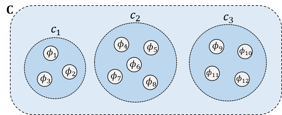
However, there is a definite relationship between computational states and physical states that always holds, for any real computing system: Namely, each well-defined computational state $c_{i}$ necessarily corresponds to a disjoint subset of some set $\mathbf{\Phi}$ of physical states. (See Fig. 2.) In other words, there is always some set $\mathbf{\Phi}$ of physical states, such that for each $c_{i}\in\mathbf{C}$, we can make the identification $c_{i}\subseteq\mathbf{\Phi}$, and for any two $i,j$, the subsets $c_{i}$ and $c_{j}$ do not overlap; $c_{i}\cap c_{j}=\varnothing$. We can also express this more concisely by saying that the set $\mathbf{C}$ of computational states is a (set-theoretic) partition of some set $\mathbf{\Phi}$ of physical states, or (if not all physical states correspond to well-defined computational states) of one of its proper subsets.

Figure 2: Physical and computational states. Example of a computational state space $\mathbf{C}=\{c_{1},\,c_{2},\,c_{3}\}$ with 3 distinct computational states, where each state $c_{i}$ is identified with a corresponding distinct subset $c_{i}=\Phi_{i}\subseteq\mathbf{\Phi}=\{\phi_{1},\,\phi_{2},\,\ldots,\,\phi_{12},\,\dots\}$ of a full set $\mathbf{\Phi}$ of all possible physical microstates of the computer (or some larger physical environment within which it is contained). Typically in practice, the number of distinguishable microstates per computational state would be astronomically large.

The reason why this must be the case is that, in order for a computational state $c_{i}$ to be well-defined, from a physical perspective, it must be possible, at least in principle, to reliably determine what the computational state is, given some conceptually-possible measurement process (i.e., some quantum-mechanical observable operator), which implies that there is some basis (implying a set of physical states $\mathbf{\Phi}$) for which, if we measure the state in that basis, we will obtain a definite answer (a specific physical state $\phi_{j}\in\mathbf{\Phi}$) that reliably reveals whether the computational state was $c_{i}$, or not. Thus, the set of $\phi_{j}$ in this basis that would reliably imply that the computational state is $c_{i}$ may be identified with $c_{i}$. This observation is very, very important: It is why information entropy (in Shannon’s conception) and physical entropy end up being fundamentally connected, as we will see.

Note that the above definition works even in the case of a quantum computer operating on any reliably-distinguishable set of input computational states, since even at any arbitrary point in the middle of a quantum computation, after some unitary time-evolution $U$ has been applied, there is always still some basis in which you could measure the computer’s physical state such that, in principle, the original input state could be reliably determined (e.g., at minimum, in principle you could always apply $U^{-1}$ to get back to the initial state before doing the measurement).

3.2.3 Computational and physical entropy.

The above observation now lets us see why the information-theoretic entropy of a probability distribution over computational states is necessarily fundamentally connected with physical entropy: Because the probability of a computational state is simply the sum of the probabilities of the corresponding physical microstates. Let $P(c_{j})$ denote the probability of the computational state $c_{j}$, and let $p_{i}=p(\phi_{i})$ denote the probability of the physical state $\phi_{i}$. Then we have:

$$P(c_{j})=\sum_{\phi_{i}\in c_{j}}p_{i}.$$ (17)

Why must this be the case? Because no other possibility is epistemologically self-consistent. Because, given that the physical state is $\phi_{i}$, and that $\phi_{i}\in c_{j}$, it must be the case that the computational state is $c_{j}$, by definition. Thus, all of the probability mass associated with the physical states $\phi_{i}\in c_{j}$ contributes to the probability mass associated with $c_{j}$ (and nothing else does).

Now, the derived probability distribution $P(c_{j})$ over the computational states $c_{j}$ implies a corresponding entropy $H(C)$ (the “information entropy”) for the computational state $C$, considered as a discrete variable. Similarly, the probability distribution $p(\phi_{i})$ over the physical states $\phi_{i}$ implies a corresponding entropy $S(\Phi)$ (the “physical entropy”) for the physical state $\Phi$, considered as a discrete variable. These two entropies necessarily have an exact and well-defined relationship to each other. This is because the probability distribution $p(\phi_{i})$ over the physical states also acts as a joint distribution over the physical and computational states, because the computational state space is just a partition of the physical state space. So, each physical state $\phi_{i}$ can thus also be identified with a pair $(\phi_{i},c_{j})$ of the values of these two discrete variables $\Phi,C$. Thus, the conditional entropy theorem applies, and we can always write the following Fundamental Theorem of the Thermodynamics of Computation:

$$S(\Phi)=H(C)+S(\Phi|C).$$ (18)

In other words, the (total) physical entropy $S(\Phi)$ is exactly equal to the information entropy $H(C)$ of the computational state, plus the conditional entropy $S(\Phi|C)$ of the physical state, conditioned on the computational state—this just means, recall, the entropy that we would expect the physical state $\Phi$ to still have, if we were to learn the exact value of the computational state $C$. This follows rigorously from the conditional entropy theorem (i.e., the derivation of the chain rule of conditional entropy).

As a convenient shorthand, we will call $S(\Phi|C)$ the non-computational entropy $S_{\mathrm{nc}}(\Phi)$ in contexts where the computational state variable $C$ is understood. Thus, in such contexts, the Fundamental Theorem (eq. 18) may also be written:

$$S(\Phi)=H(C)+S_{\mathrm{nc}}(\Phi).$$ (19)

Another equivalent statement to eq. 18 is that $H(C)=I(\Phi;C)$, that is to say, the information entropy of the computational state is equal to the mutual information between the physical and computational state variables. This is obviously true, since the computational state can be thought of as being the state of an abstract physical system (“the computational system”) that is just subsystem of the underlying physical system—so that, clearly, all of our information about the computational system is redundant with our information about the physical system (since the computational system is just a part of the physical system).

Simple as it is, we will call eq. 18 (or 19) the Fundamental Theorem of the Thermodynamics of Computation, because essentially everything else that is important to understand about the subject rests upon it in some way.

3.2.4 Visual proof of the Fundamental Theorem.

Rather than reviewing the algebraic derivation that proves eq. 18 formally, we will describe a simple visual representation of the theorem that makes plain why it is true. This is where the heaviness concept that we mentioned in §2.1 becomes useful. We saw in Fig. 1(a) that the heaviness or psychological weight of an outcome (value of a variable) can be visualized as a rectangle whose width is proportional to its probability, and whose height is proportional to its surprise or log-improbability. Consider this rectangle, now, as one upwards-pointing branch of a tree, having one branch for each outcome. The total heaviness of all the branches then corresponds to the entropy of the given probability distribution.

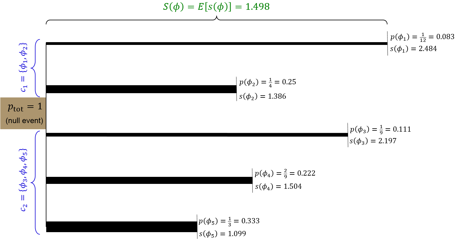
Thus, for example, in Fig. 3(b), we see a tree representing a probability distribution over 5 physical states $\mathbf{\Phi}=\{\phi_{1},\,\phi_{2},\,\ldots,\,\phi_{5}\}$, where the probabilities are $p_{1}=1/12,p_{2}=1/4,p_{3}=1/9,p_{4}=2/9,p_{5}=1/3$. (The aspect ratio for the diagram is arbitrary, but the relative line heights and the relative line widths are otherwise to scale.)

Figure 3: Graphical illustration of the Fundamental Theorem of the Thermodynamics of Computation. (a) Example of a computational state space $\mathbf{C}=\{\,\{\phi_{1},\phi_{2}\},\,\{\phi_{3},\phi_{4},\phi_{5}\}\,\}$ constructed as a partition of a set $\mathbf{\Phi}$ of 5 physical states $\{\phi_{1},\,\ldots,\,\phi_{5}\}$. (b) Tree representation of a probability distribution over $\phi_{1},\,\ldots,\,\phi_{5}$ given as 1/12, 1/4, 1/9, 2/9, 1/3. (c)-(d) Merging of the lower parts of the branches to create “trunk” branches for the computational states, and “stem” branches to represent the conditional probability distribution over the physical states, given the computational states. As discussed in the text, it is easy to see from the definition of conditional probability that the total heaviness (area) of all branches remains the same before and after the merge, and thus the Fundamental Theorem of the Thermodynamics of Computation (eq. 18) follows.

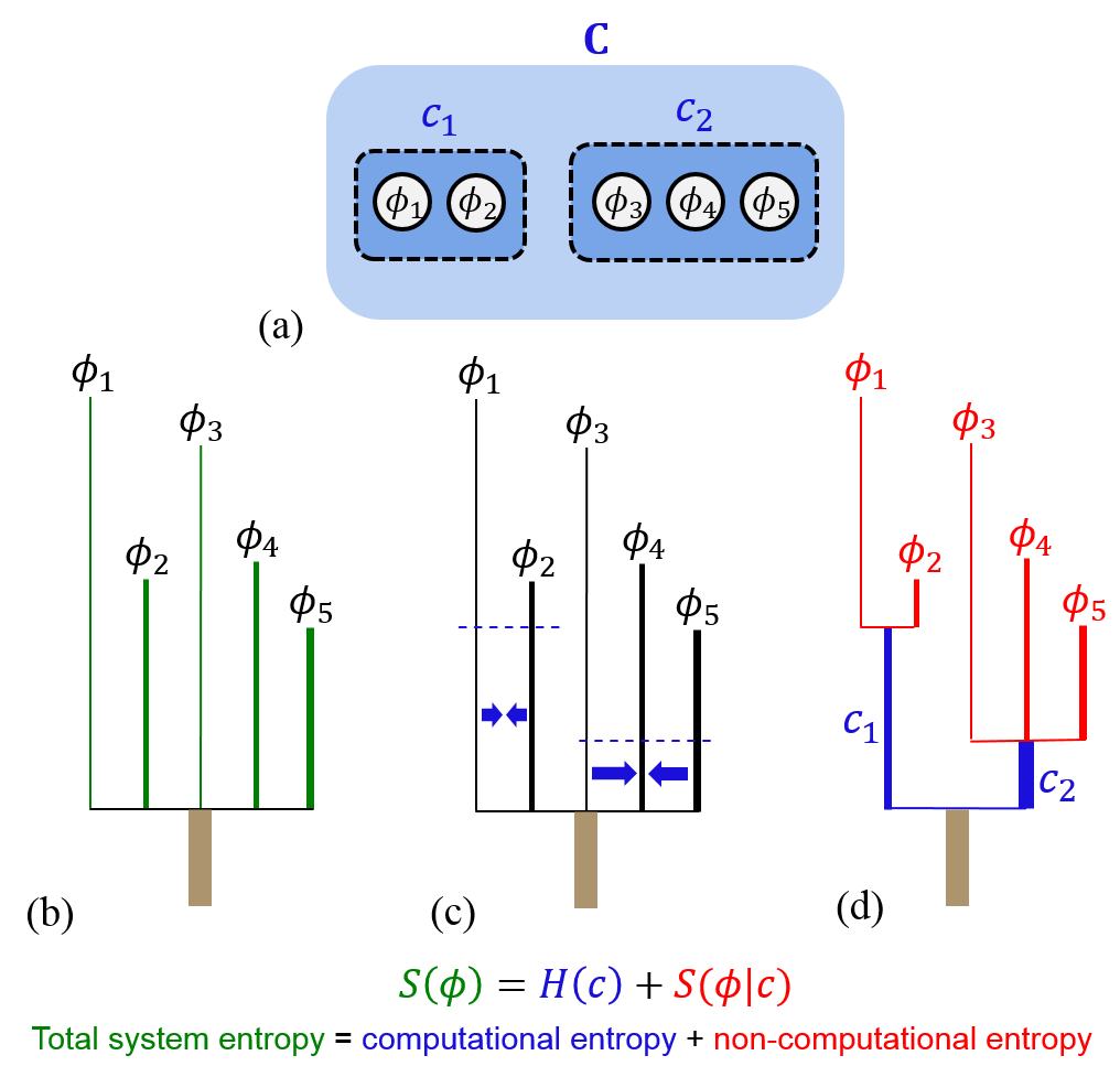
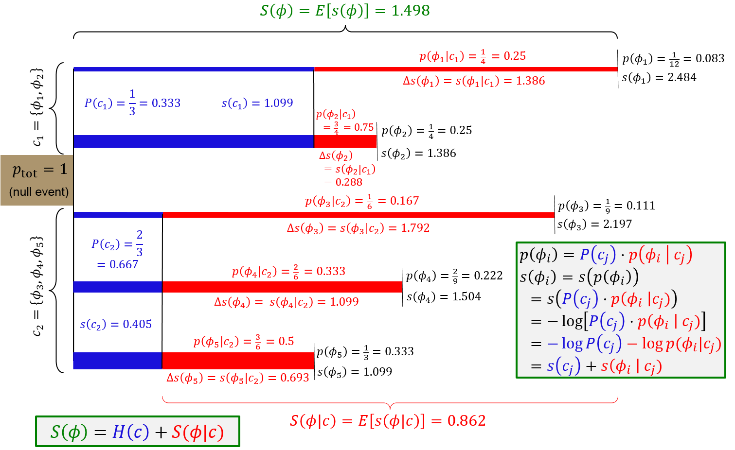
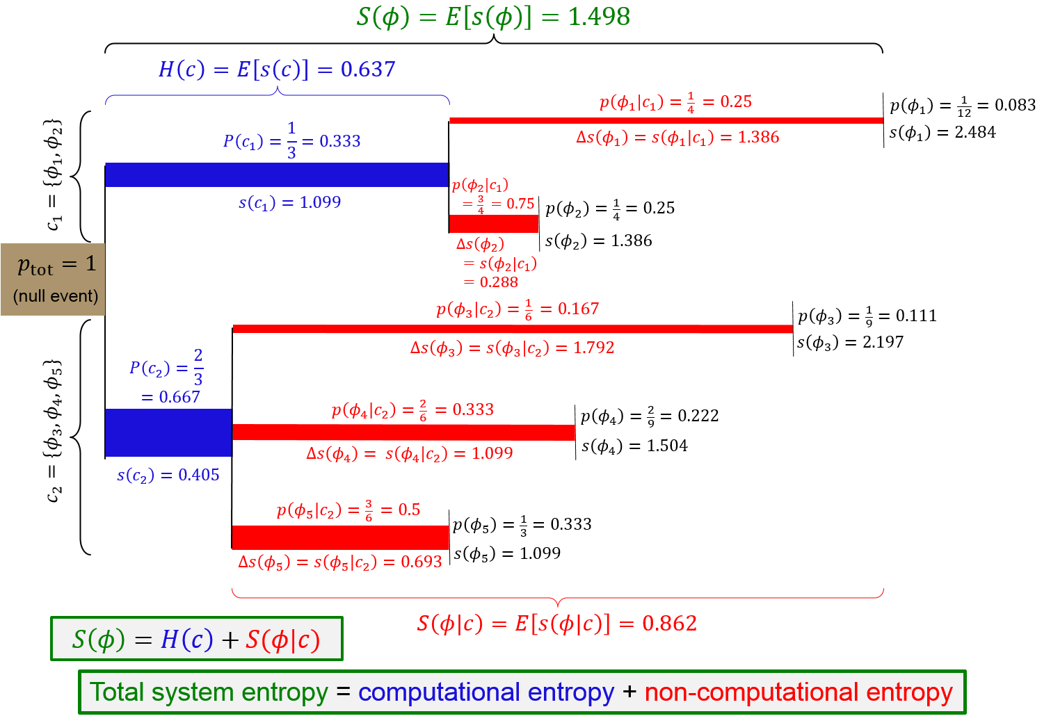
Now, if we wish to group individual outcomes into larger events corresponding to states of subsystems, like we do when we group physical states into computational states, we can represent this graphically by merging portions of branches into thicker branches. So, for example, suppose that, as in Fig. 3(a), the physical states $\{\phi_{1},\,\phi_{2}\}$ are to be grouped into the computational state $c_{1}$, and the physical states $\{\phi_{3},\,\phi_{4},\,\phi_{5}\}$ are to be grouped into the computational state $c_{2}$. Then we can use the derived probabilities $P(c_{i})$ of the larger events $c_{i}$, together with the conditional probabilities $p(\phi_{j}|c_{i})=p(\phi_{j})/P(c_{i})$ for the smaller events $\phi_{j}$, to create appropriate “trunk” (blue) and “stem” (red) branches (see Fig. 3(c,d)) for the micro-events $\phi_{j}$. Note that the original probability is just the product of the new ones, $p(\phi_{j})=P(c_{i})\cdot p(\phi_{j}|c_{i})$, and since the logarithm of a product is a sum, the length of the original branch is just the sum of the lengths of its corresponding trunk and the resulting stem. In other words, the heights of all of the leaves of the tree are unchanged. And since probabilities of mutually-exclusive sub-events add, the total width of each trunk is the same as the total width of the branches it is merged from. So, it is easy to see visually that the total area or heaviness of this two-dimensional tree is the same after the merge. Thus, the total entropy is the same. Thus, the entropy of the computational state (blue) plus the entropy of the non-computational state (red), or in other words the entropy of the physical state conditioned on the computational state, is the same as the total entropy of the physical state (green). This is exactly what the Fundamental Theorem of the Thermodynamics of Computation is saying.

The appendix gives additional numerical and analytical details for this example.

3.3 Physical Time-Evolution and Computational Operations

We now discuss how physical states dynamically evolve (transform to new states) over time, and relate this to our concept of computational operations from §2.3. We begin by discussing how the law of non-decreasing entropy originally noticed by Clausius (the $2^{\mathrm{nd}}$ Law of Thermodynamics) follows as a direct logical consequence of the time-reversibility (injectivity) of microscopic dynamics.

3.3.1 The reversibility of microphysics.

For our purposes, the most important thing to know about the dynamical behavior of low-level physical states is that they evolve reversibly (and deterministically), meaning, via bijective (one-to-one and onto) transformations of old state to new state.

Formally, in quantum theory [28, 29], over any time interval $\mathrm{\Delta}t$, quantum states (mathematically represented as vectors in Hilbert space) are transformed to new state vectors by multiplying them by what in linear algebra are called unitary matrices, i.e. invertible linear operators that preserve vector norms (lengths). Specifically, in any closed quantum system, the time-evolution operator is given by $U(\mathrm{\Delta}t)=\mathrm{e}^{-\mathrm{i}\mathrm{\Delta}tH/\hbar}$, where $\mathrm{i}=\sqrt{-1}$ is the imaginary unit, $\hbar=h/2\pi$ is the reduced Planck’s constant, and $H$ is the Hamiltonian, an Hermitian operator that is the total-energy observable of the system.

For our purposes, the key point is that it is a mathematical property of unitary transformations that they preserve the inner product between any two vectors (a complex analogue of a geometric dot product), which implies they preserve the angle (in Hilbert space) between the vectors. This is important because any two quantum state vectors $\ket{\psi_{1}},\,\ket{\psi_{2}}$ represent physically distinguishable states if and only if they are orthogonal vectors, i.e. at right angles to each other, meaning that their inner product $\braket{\psi_{1}}{\psi_{2}}=0$. Thus, since unitary transformations preserve angles, distinguishable quantum states always remain distinguishable over time. So, if we identify our set of physical states $\{\phi_{i}\}$ with an orthonormal set $\{\ket{\psi_{i}}\}$ of quantum state vectors, it’s guaranteed that these states transform one-to-one (injectively) onto a new set of mutually orthogonal states over any given time interval $\mathrm{\Delta}t$.

Setting aside the full linear algebraic machinery of quantum mechanics, we can summarize the important points about the situation for our purposes by saying that we have, for any given time $t\in\mathbb{R}$, a corresponding physical state space $\mathbf{\Phi}(t)$, such that, for any pair of times $s,t\in\mathbb{R}$, the dynamics among the states between these times is fully described by a total, bijective (one-to-one and onto) function $D(s,t)=D_{s}^{t}:\mathbf{\Phi}(s)\rightarrow\mathbf{\Phi}(t)$ mapping states at time $s$ to the states that they evolve to/from (depending on the sign of the time interval $\mathrm{\Delta}t=t-s$) at $t$. Further, for all $t\in\mathbb{R}$, $D_{t}^{t}$ is the identity function, and the dynamics is self-consistent, in the sense that for all $s,t,u\in\mathbb{R}$, $D_{t}^{u}\circ D_{s}^{t}=D_{s}^{u}$, i.e., the transformation that obtains from time $s$ to $t$, followed by the one from $t$ to $u$, is the same as the one from $s$ to $u$.

3.3.2 The $2^{\mathbf{nd}}$ Law as a consequence of the reversibility of microphysics.

As we mentioned briefly in [11, 12, 13], it is easy to see that in any such bijective dynamics, any initial probability distribution $P(t)=p(\phi_{i}(t))$ over the physical states at time $t$ will be transformed, over any time interval $\mathrm{\Delta}t\in\mathbb{R}$, to what is essentially the same distribution over the corresponding new states,

$$P(t+\mathrm{\Delta}t)=p(\phi_{i}(t+\mathrm{\Delta}t))=p\left(D_{t+\mathrm{\Delta}t}^{t}(\phi_{i}(t+\mathrm{\Delta}t))\right),$$ (20)

in other words, the probability of any state at time $t+\mathrm{\Delta}t$ is identical to the probability of the state that it came from at time $t$. Thus, the entropy $S(P)$ of the probability distribution is exactly preserved; $S(P(t_{1}))=S(P(t_{2}))$ for all $t_{1},t_{2}\in\mathbb{R}$. So, when we know the precise microscopic dynamics $D$ and can exactly track its effects, entropy never increases or decreases (Fig. 4(a)).

Figure 4: The $2^{\mathbf{nd}}$ Law from bijective microphysical dynamics. (a) Example of a bijective dynamics for a simple system with 3 physical states. The new states have identical probabilities, and thus entropy is unchanged. (b) If the dynamics was not injective, the $2^{\mathrm{nd}}$ Law of Thermodynamics would be false. If two states ever combined, then the illustrated initial probability distribution would be changed to one of lower entropy. This is true whenever the probabilities of two merged states are both nonzero. (c) Entropy increases because we don’t have exact knowledge of the microscopic bijective dynamics, and/or don’t have the modeling capability to track its consequences in full detail, so we replace the true dynamics with a stochastic one that expresses our ignorance and/or incompetence. In the illustration, we treat the upwards-sloped and downwards-sloped injective transformations as equally probable, resulting in a final distribution that has greater entropy than the initial one.

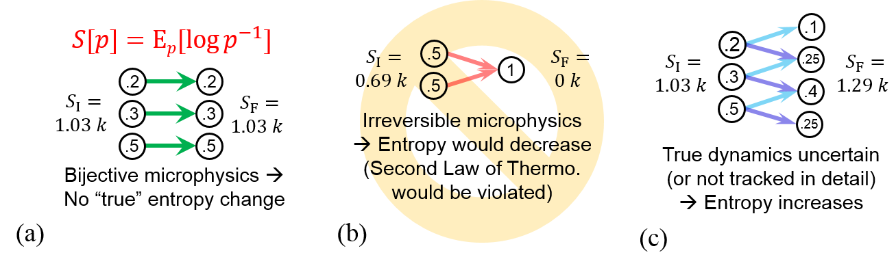
It is easy to see that the fact of the reversibility (bijectivity) of microphysics is actually a logical consequence of the Second Law of Thermodynamics (Fig. 4(b)), since if the dynamics $D$ was not always a one-to-one function, we would have two distinct physical states $\phi_{1},\phi_{2}$ at some time $t$ that were both taken to the same state $\phi$ at some later time $t+\mathrm{\Delta}t$ by the transformation $D_{t}^{t+\mathrm{\Delta}t}$; their probabilities would be combined, and (it is easy to show), the heaviness (contribution to the total entropy) from the new state, $h(\phi)$, would necessarily be less than the sum of the heavinesses of the old states, $h(\phi_{1})+h(\phi_{2})$. (This follows from the fact that the heaviness function is concave-down; see Fig. 1(b).) Thus, total entropy would be decreased, and the Second Law would be false.

How, then, can entropy increase? Well, in practice, we do not know the entire dynamics $D$, or, even when we do, tracking its full consequences in microscopic detail would be beyond our capacity to accurately model. If the dynamics $D$ is uncertain, or is simplified for modeling purposes by replacing it with a less-detailed model, then, even though we know that the true underlying dynamics (whatever it is) must be one-to-one, the fact that in practice we have to replace the true dynamics with a statistical ensemble over possible future dynamical behaviors implies that, in this simplified model, the entropy will be seen as increasing. This is illustrated in Fig. 4(c) for a simple case. In this example, if the three states on the left (with probabilities 0.2, 0.3, 0.5) would transform bijectively to new states (on the right), but we had complete uncertainty about whether they would transform to the upper 3 states (upwards-sloping light blue arrows), or to the lower 3 states (downwards-sloping purple arrows), we would end up with a probability distribution over final states exhibiting greater entropy (in this case, by $0.26k$) than the initial distribution.

3.3.3 Computational operations and entropic dynamics.

Let us now see what the bijective dynamics of microphysics implies about how entropy is transferred in computational operations. First, we will expand our concept of a computational state $c_{i}$ slightly, to account for the fact that the physical state space $\mathbf{\Phi}(t)$ will in general be changing over time, as individual states evolve according to the dynamics $D$. We will say that at any given time $t\in\mathbb{R}$, there is a computational state space $\mathbf{C}(t)=\{c_{i}(t)\}$ such that each computational state $c_{i}(t)\in\mathbf{C}(t)$ is a distinct subset of the physical state space $\mathbf{\Phi}(t)$ at that time, that is, $c_{i}(t)\subseteq\mathbf{\Phi}(t)$, and $c_{i}(t)\cap c_{j}(t)=\varnothing$ for all $i\neq j$.

Correspondingly, we must expand our notion of applying a computational operation $O$ in a computational scenario $\mathcal{C}=(O,P_{\mathrm{I}})$ to account for the fact that the computational states may be described differently, in terms of physical states, depending on exactly when the operation starts and ends. For this, we annotate the operation with its start and end times $s,t\in\mathbb{R}$, like $O_{s}^{t}$. This notation then denotes that when the operation $O$ is applied from time $s$ to time $t$, the initial state $c_{\mathrm{I}i}=c_{i}(s)$ at time $s$ is mapped to final state $c_{\mathrm{F}j}=c_{j}(t)$ at time $t$ with probability $P_{i}(c_{j})=O(c_{i})(c_{j})$, where here, $c_{i},c_{j}$ label the time-independent computational states relative to which the original version of the operation $O$ was defined.

Now, let us examine more closely the consequences of applying a general computational operation $O_{s}^{t}$ from time $s$ to $t$, in the context of an underlying physical dynamics $D$ that is bijective.

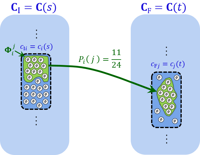
First, consider cases where $O$ is stochastic, so that there are computational state pairs $c_{i},c_{j}$ such that $0<P_{i}(c_{j})<1$; that is, a certain nonzero amount, but not all, of the probability mass from state $c_{i}$ at the initial time $s$ ends up in state $c_{j}$ at the final time $t$. In order for this to be the case, when nothing is known about the initial physical state $\Phi(s)$ beyond what is implied by the initial computational state $C(s),$ then $c_{i}(s)$ must correspond to a subset of $\mathbf{\Phi}(s)$ of initial physical states that itself has a proper subset $\Phi_{i}^{j}\subset c_{i}(s)$ consisting of states that will be mapped by the dynamics $D_{s}^{t}$ into the final state $c_{j}(t)$, and whose probability mass is a fraction $P_{i}(c_{j})$ of the total. Or, in equations,

$$\Phi_{i}^{j} = \{\;\;\phi_{k}(s)\in c_{i}(s)\;\;|\;\;D_{s}^{t}(\phi_{k}(s))\in c_{j}(t)\;\;\}$$ (21)

$$\frac{|\Phi_{i}^{j}|}{|c_{i}(s)|} = P_{i}(c_{j}).$$ (22)

To explain eq. 22, given a maximum-entropy conditional probability distribution $P(\Phi(s)\,|\,C(s))$, all of the microstates $\phi_{k}(s)$ in the given initial computational state $c_{i}(s)$ must be equally likely, so the ratio $|\Phi_{i}^{j}|/|c_{i}(s)|$ of the respective set cardinalities suffices to quantify $P(\phi\in\Phi_{i}^{j}\,|\,\phi\in c_{i}(s))$, the fraction of the total probability mass in $c_{i}(s)$ that is also in $\Phi_{i}^{j}$. See Fig. 5 for an illustration.

Figure 5: Stochastic computation under bijective dynamics. This diagram shows the relation of a stochastic computational operation to bijective microphysics. Illustrated are an initial computational state space $\mathbf{C}_{\mathrm{I}}=\mathbf{C}(s)$ at time $s\in\mathbb{R}$ and a final computational state space $\mathbf{C}_{\mathrm{F}}=\mathbf{C}(t)$ at some later time $t>s.$ Suppose that a stochastic computational operation $O_{s}^{t}$ is to be performed such that the probability of going from some particular initial computational state $c_{\mathrm{I}i}=c_{i}(s)$ at time $s$ to the final state $c_{\mathrm{F}j}=c_{j}(t)$ at time $t$ should be $P_{i}(j)=11/24=0.458\bar{3}$, and let the initial state of knowledge be one in which the conditional probability distribution over the initial physical state $\Phi(s)$ given the computational state $C(s)$ is at maximum conditional entropy (i.e., the only information known about the physical state $\Phi(s)$ is the mutual information between the computational and physical state, which is the information about the computational state, $K(\Phi(s))=I(\Phi(s);C(s))=K(C(s))$). Then it follows that all $\phi_{k}\in c_{j}(t)$ are equally likely, and thus a fraction $11/24$ of these physical states must be in the subset $\Phi_{i}^{j}\subset c_{i}(s)$ that will be mapped into $c_{j}(t)$ by the micro-physical dynamics $D(s,t)$ operating between times $s$ and $t$. Note that here, $c_{\mathrm{I}i}$ has only 24 microstates, and so exactly 11 of them must go to $c_{\mathrm{F}j}$. More realistically, there would be an astronomically-large number of microstates per computational state.

Finally, let’s examine the entropic implications of performing an irreversible computational operation $O_{s}^{t}$, which by definition means an operation in which some final computational state $c_{\mathrm{F}k}=c_{k}(t)$ at time $t$ has some nonzero probability of being reached from more than one initial computational state at time $s$, for example from both $c_{\mathrm{I}i}=c_{i}(s)$ and $c_{\mathrm{I}j}=c_{j}(s)$ for some $i\neq j$. Irreversible operations may generally reduce the entropy $H(C)$ of the computational state, as can be seen by setting the initial probabilities of both $c_{\mathrm{I}i}$ and $c_{\mathrm{I}j}$ to nonzero values (and all other initial-state probabilities to 0). However, irreversible computational operations may still be implemented in bijective physics, but only by correspondingly increasing the entropy $S_{\mathrm{nc}}(\Phi)=S(\Phi|C)$ of the non-computational part of the state. Why? Because the Fundamental Theorem of the Thermodynamics of Computation (eq. 19), together with the bijectivity of microphysics, ensures that the sum of computational and non-computational entropies will be constant (or at least, non-decreasing, if the dynamics $D$ is uncertain).

For the case of a deterministic (non-stochastic) operation $O_{s}^{t}$, we can summarize the implications of the above observation very simply, by saying that between times $s$ and $t$, the required change (increase) $\mathrm{\Delta}S_{\mathrm{nc}}$ in the non-computational entropy $S_{\mathrm{nc}}(\Phi)$ of the physical state $\Phi$ is given by the negative of the (negative) change (decrease) $\mathrm{\Delta}H(C)$ in the entropy of the computational state $C$ (the computational entropy); this is true in any statistical context, with any initial distribution $P_{\mathrm{I}}(C_{\mathrm{I}})$ over the initial computational state variable $C_{\mathrm{I}}=C(s)$:

$$\mathrm{\Delta}S_{\mathrm{nc}}(\Phi)=-\mathrm{\Delta}H(C)=H(C_{\mathrm{I}})-H(C_{\mathrm{F}})$$ (23)

This observation is illustrated by the example in Fig. 6.

Figure 6: Entropy ejection from the computational state. Illustration of a deterministic, logically irreversible computational operation in bijective microphysics. Illustrated is an initial computational state space $\mathbf{C}_{\mathrm{I}}=\mathbf{C}(s)$ at time $s$ consisting of two possible initial computational states $c_{\mathrm{I}1}=c_{1}(s)$ and $c_{\mathrm{I}2}=c_{2}(s)$, and a final computational state space $\mathbf{C}_{\mathrm{F}}=\mathbf{C}(t)$ at time $t>s$ consisting of just one final computational state $c_{\mathrm{F}1}=c_{1}(t)$. The desired computational operation $O_{s}^{t}$ is one that maps both $c_{\mathrm{I}1}$ and $c_{\mathrm{I}2}$ to $c_{\mathrm{F}1}$ with certainty. It follows from this that if the initial probability distribution $P_{\mathrm{I}}(C_{\mathrm{I}})$ over the computational states has some nonzero entropy $H(C_{\mathrm{I}})$, then the entropy over the computational state will be reduced by an amount $\mathrm{\Delta}H(C)=-H(C_{\mathrm{I}})$, that is, to 0, and therefore (by the Fundamental Theorem of the Thermodynamics of Computation, and bijectivity), the entropy $S_{\mathrm{nc}}(\Phi)$ of the non-computational state will have to be increased correspondingly, i.e., $\mathrm{\Delta}S_{\mathrm{nc}}(\Phi)=-\mathrm{\Delta}H(C)=H(C_{\mathrm{I}})$. We can say that all of the entropy in the computational subsystem has been ejected into the non-computational subsystem. The figure shows state probabilities for a case where the initial computational entropy is $H_{\mathrm{I}}=H(C_{\mathrm{I}})=\log 2=1\,\mathrm{bit}\approx 0.69k$, and the initial non-computational entropy was some arbitrary value (here about $0.59k$).

3.3.4 Intake of entropy by stochastic randomization.

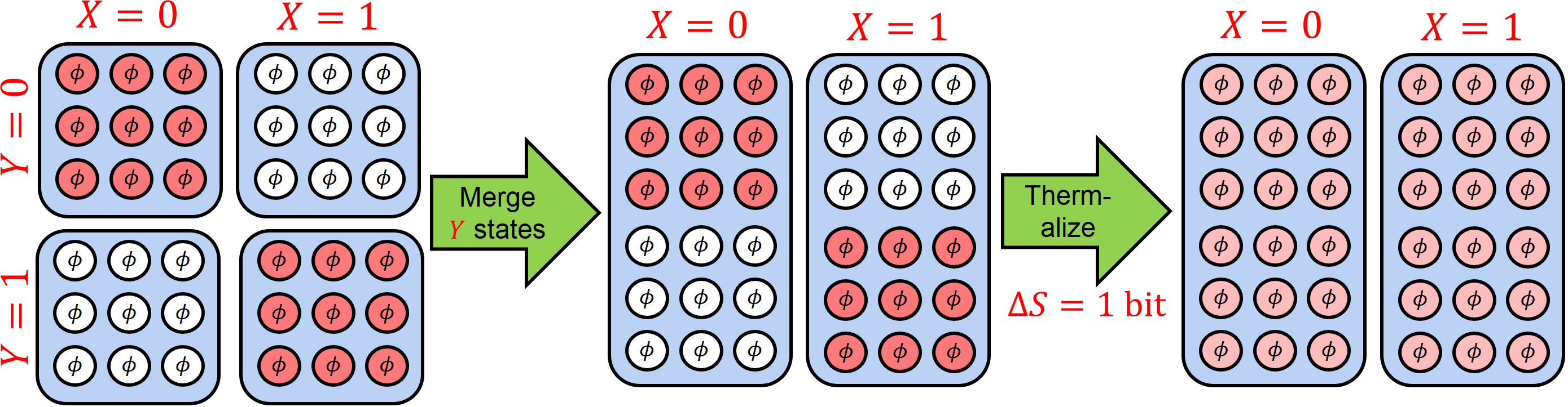
The above constitutes an important part of the argument for Landauer’s Principle. However, this argument is not yet complete, for the following reason. Processes such as the one illustrated in Fig. 6 are actually thermodynamically reversible. What do we get if we reverse in time a deterministic, logically irreversible process (by exchanging its initial and final times $s,t$)? We exactly get a stochastic, reversible process, which corresponds to performing a measurement on the physical state. The time-reverse of Fig. 6, in particular, is a process that takes the final computational state $c_{\mathrm{F}1}$ stochastically back to either $c_{\mathrm{I1}}$ or $c_{\mathrm{I2}}$, with a probability distribution $P_{i}(j)$ that depends on the probability distribution over the physical states $\phi_{k}\in c_{\mathrm{F}1}$. For a uniform (maximum-entropy) distribution over physical states, the probabilities of returning to the initial states $c_{\mathrm{I1}}$ and $c_{\mathrm{I2}}$ would both be 0.5. This is the same as the distribution we started with, so if we performed the process in Fig. 6 forwards and then in reverse, the entropy of the computational state $H(C_{\mathrm{I}})$ would be unchanged. However, if we allowed the physical states making up $c_{\mathrm{F}1}$ to be randomly reshuffled before the reversal, the final computational state might not be the same as the initial one. Thus, such an operation (including the intermediate random permutation of the physical states) would be stochastic and logically irreversible, yet it could preserve the entropy $H(C_{\mathrm{I}})$ of the computational state overall. (See Fig. 7.) It could also leave the non-computational entropy $S_{\mathrm{nc}}(\Phi_{\mathrm{I}})$ of the physical state unchanged; for example, this would necessarily be the case whenever $S_{\mathrm{nc}}(\Phi)$ was already maximal initially, the initial and final computational entropies were maximal, and the detailed physical state was not further measured.

Figure 7: Illustration of conjoining a deterministic, logically irreversible computational operation with its time-reverse, which is a stochastic, logically reversible computational operation. In between, in this example we assume that a completely unknown physical dynamics $\tilde{D}(t_{2},t_{3})$ occurs, which totally randomizes the physical state, yielding a maximum-entropy distribution over the physical states at time $t_{3}$. In this example, the overall effect of the entire process is that the entropy of the computational state remains unchanged at $H(C)=1\,\mathrm{bit}$, and the entropy of the non-computational state has been increased from $\sim 0.85$ bits to 1 bit. However, note that if the initial non-computational entropy had already been maximal (1 bit), then it could not have increased further. This illustrates that logically irreversible operations on isolated, unknown computational bits do not necessarily cause entropy increase, despite stochastic evolution of the environment; the ejection of computational entropy to non-computational form can sometimes be undone by subsequent stochastic operations (measurements). However, we will later see that when logically irreversible operations are performed in computational scenarios featuring multiple correlated computational state variables, the requirement for a permanent entropy increase as per Landauer is recovered.

3.3.5 Role of correlations.

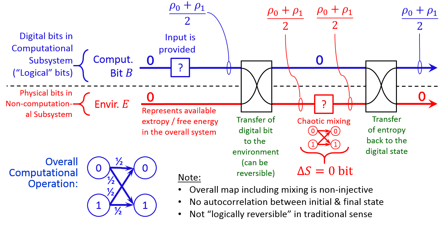
Thus, entropy contained in isolated, random computational bits, not having any correlations to any other available information, can be ejected to the environment in a thermodynamically reversible way; another view of this process is illustrated in Fig. 8. There, the merging/splitting of computational states is represented as an exchange of information between computational and non-computational subsystems.

Figure 8: Thermodynamically reversible erasure of an unknown, uncorrelated bit. Spacetime diagram showing an operation sequence for the thermodynamically reversible erasure and re-randomization of an isolated digital bit whose initial value is unknown and uncorrelated with any other available information. For simplicity, we imagine that the computational and non-computational subsystems each have only 1 bit of information capacity (2 distinct states). Initially, an input mechanism obtains some unknown bit-value from the external environment, after which the computational bit $B$ has a mixed state with 1 bit of entropy, representable by the density matrix $(\rho_{0}+\rho_{1})/2$, where $\rho_{i}$ is a matrix representing the state where bit $B$ has the unconditional value $v_{i}=i$. Suppose the environment bit $E$ is originally in a “cold,” zero-entropy state. We can reversibly swap bits $B$ and $E$, moving the entropy from the computational subsystem to the non-computational one. After this, the environment $E$ can undergo a stochastic evolution that randomly scrambles its state—but this does not increase its entropy, since it was already maximal. Finally, we can reversibly transfer the bit of entropy back to the digital state. Overall, this process entails no net increase in entropy, yet is logically irreversible, due to the stochastic evolution.

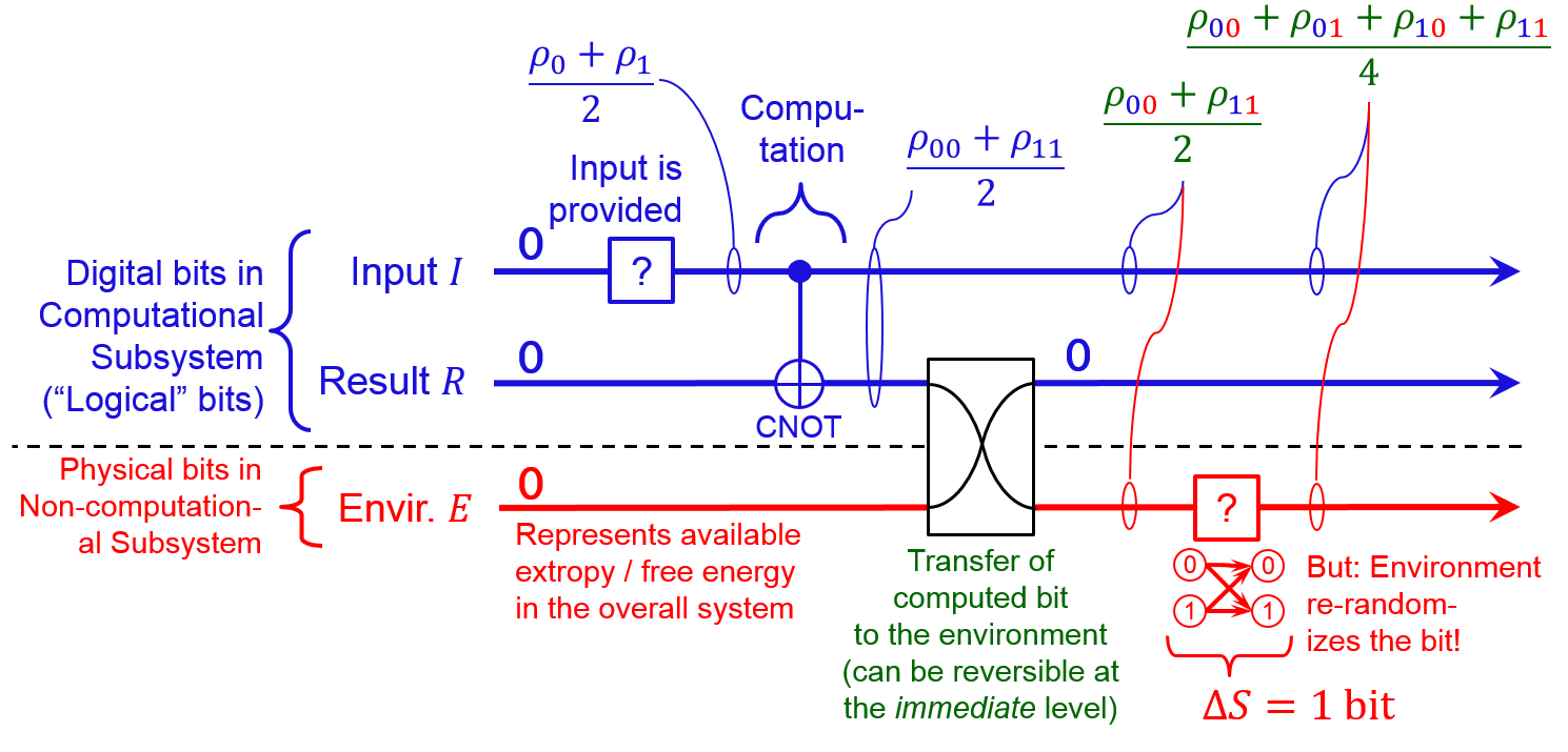
However, in those examples, the fact that the digital bit that is being erased is initially uncorrelated with others is important. Because the bit was uncorrelated with others, and its initial value was unknown, re-randomizing its value through the erasure/unerasure process does not actually decrease our known information, or increase entropy. However, if the bit was initially correlated with others, in the sense of sharing mutual information with them, then the situation is different. This would be the case for any bits that are deterministically computed from others (see, e.g., Fig. 9). In this case, after the computed bit has been ejected to the environment, and is then randomized by the stochastic evolution of the environment, the prior correlation is lost, and total entropy is increased. This consequence is truly unavoidable whenever we cannot track the exact microscopic dynamics of the environment, which is (by definition) always the case for a thermal environment, given that we do not have complete knowledge of (and capacity to keep track of) the microstate of the universe, nor do we know the complete laws of physics, the exact values of coupling constants, etc.

Figure 9: Logically irreversible, oblivious erasure of a correlated bit. Spacetime diagram showing an operation sequence for the thermodynamically irreversible, oblivious erasure of a computed bit whose value is correlated with other available information. Here, there are 2 bits $I,R$ in the computational subsystem, and 1 bit $E$ in the non-computational one. As in Fig. 8, an unknown input bit value is provided on the input bit $I$, and $R$ is initially $v_{0}=0$, and then a controlled-NOT operation is performed between $I$ and $R$. Now $I$ and $R$ are correlated (in the sense that they share 1 bit of mutual information), and their joint mixed state can be represented by the density matrix $(\rho_{00}+\rho_{11})/2$, where $\rho_{ij}$ is a density matrix representing the state where $I=v_{i}$ and $R=v_{j}$ with certainty. Now, we can reversibly transfer one of those bits $R$ as before, but now, when the environment re-randomizes its bit $E$, this loses the correlation between $I$ and $E$, and our knowledge about the state is now described by the density matrix $(\rho_{00}+\rho_{01}+\rho_{10}+\rho_{11})/4$, which has 2 bits of entropy. This represents a permanent entropy increase of $\mathrm{\Delta}S=1\,\mathrm{bit}$. See also Fig. 10.

A more detailed, fully general proof of Landauer’s Principle based on these observations about correlations goes as follows. Let $X,Y$ be any two discrete random variables. For example, $Y$ could be a particular logical bit (i.e., a computational subsystem with a computational state space consisting of two distinct computational states) or set of bits of interest in a computer. And $X$ could be the rest of the logical bits in the computer.

Now, given any joint probability distribution $P(X,Y)$ over these two variables, we know, as a matter of definition, that the mutual information between $X$ and $Y$ is given by $I(X;Y)=H(X)+H(Y)-H(X,Y)$ (eq. 14), where $H(X,Y)$ is just the usual von Neumann/Shannon entropy of the joint distribution $P(X,Y)$, and where $H(X),H(Y)$ are just the usual (reduced) entropies of the respective subsystems.

Note that whenever $I(X;Y)>0$, a subsystem entropy value such as $H(Y)$ in general exaggerates the amount of independent random information that is actually in $Y$, since part of the apparent uncertainty in $Y$ is actually determined by (correlated with) $X$—namely, a part equal to the mutual information $I(X;Y)$.

We can thus usefully define a quantity which we call the independent entropy of $Y$ as

$$S_{\mathrm{ind}}(Y) = H(Y)-I(X;Y)$$ (24)

$$= H(Y|X),$$ (25)

that is, it’s just the conditional entropy of $Y$, conditioned on $X$. (Recall, this just means the expectation value of what the remaining entropy of $Y$ would be, if we were to measure $X$ and learn its value.)

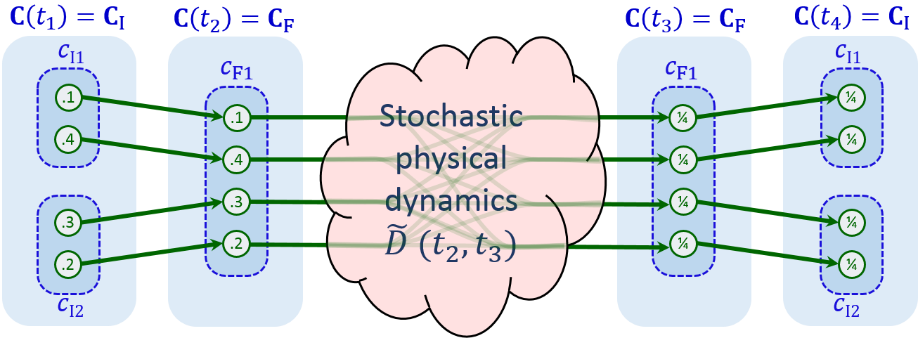
Suppose, now, that we erase $Y$ via a $local,oblivious$ mechanism—that is, one that does not depend at all on the value of $X$ (or any other system that is correlated with $Y$). Typically, this could be done in a way that is completely isolated from subsystem $X$, and does not interact at all with it. We can do this erasure as slowly as we like. Then, after waiting a bit (on a suitable thermalization timescale), we perform the reverse of this process, returning $Y$ to a state with the same subsystem entropy $H(Y)$ as it had originally; note that this is the same case that we already exemplified in Fig. 9 (with $X=I$ and $Y=R$), but in a more general context.

Note that, in this re-randomization process, it’s now impossible for that process to restore any of the correlations with $X$, since we’re not even interacting with $X$ at all in the re-randomization process (since it is equally as oblivious to $X$ as the forward process was).

Another way to look at this is that, during the period when the correlated information that was in $Y$ is instead out there in the thermal (non-computational) environment, the mutual information that the state originally had with subsystem $X$ is completely lost, it vanishes (in the sense of, degrading to entropy) over the course of that time (at or exceeding the thermalization timescale of the environment).

So in other words, at this point, despite the fact that $H(Y)$ is the same as it was originally, now all correlations with $X$ have been lost, since the thermal environment (as per the very nature of what we mean by this term) won’t have preserved those correlations in any accessible form—thus, now, $I(X;Y)=0$, and so $S_{\mathrm{ind}}(Y)=H(Y)$. In other words, the independent entropy of $Y$ has now been increased, exactly by the amount $I(X;Y)$.

Note this implies a crucial observation: Whenever any subsystem $Y$ bearing any nonzero amount of mutual information (shared with any other system $X$) is obliviously erased (without regards to $X$), this causes an increase in the total entropy of the universe equal to (at minimum) the amount of mutual information that $Y$ previously contained.

Now, suppose further that originally, $Y$ was, in fact, deterministically computed from $X$. Note this is the case for any bit in a computer, other than the input. (Even for free memory, if we assume it has been initialized to a standard state, it can be considered just a constant function of the input.)

So then, since $Y$ is just a function of $X$, clearly, $H(Y|X)=0$ initially. And, $H(Y)=I(X;Y)$. So, for example, if $Y$’s subsystem entropy is exactly 1 bit, say ($\log 2=k\ln 2$ entropy, meaning equal probability of 0 and 1), then so is its mutual information with $X$.

Thus, in such a case, erasing $Y$ (even quasistatically) and then reversing this process results in a total entropy increase of $\Delta S=1\,\mathrm{bit}=k\ln 2$, even though we have $H(Y)=1$ at both the start and end of this process. Because, the 1 bit’s worth of correlation that it had with the rest of the system has been lost. So, the new $P(X,Y)$ distribution has 1 more bit of entropy than it did previously. And, there’s been no decrease in environment entropy to make up for this (because the erasure/restoration process was done obliviously, it couldn’t take advantage of the correlation to avoid increasing the entropy of the environment while part of the correlated state was being ejected).

Another way to describe the above process is to say that obliviously erasing computed bits turns their “fake” subsystem entropy (i.e., their mutual information that they have with other systems) into real entropy, which is why total entropy increases.

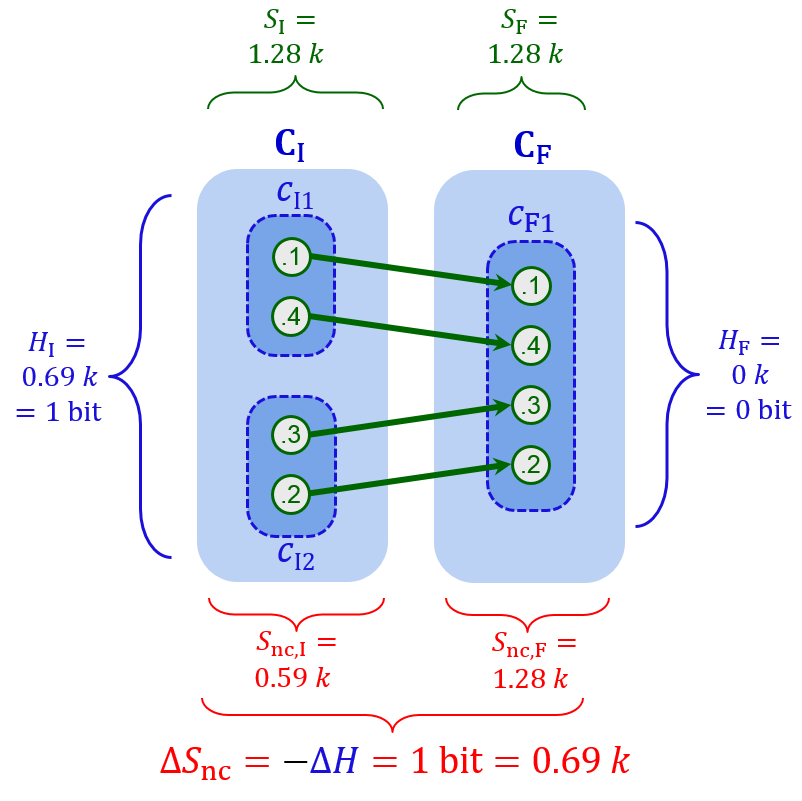
The above argument is illustrated pictorically in Fig. 10, using computational states illustrated as sets of physical states.

Figure 10: Entropy increase from thermalization of mutual information. (Left) Two perfectly-correlated computational bits $X$ and $Y$; e.g., these could be the bits $I$ and $R$ from Fig. 9. (Middle) When $Y$ is obliviously erased, this amounts to merging the two computational state spaces in each column; we can say $Y=0$ in each merged space. Note that now, there briefly exists a correlation between $X$ and the non-computational part of the physical state. (Right) Very quickly (over a thermalization timescale), we lose track of the probabilities of the different physical states making up each computational state, losing this correlation. This is where the absolute increase of total entropy from Landauer’s Principle necessarily occurs. We cannot then undo this entropy increase by simply reversing the first step (un-merging the $Y$ states), because the correlation information has already been irrevocably lost by this point.

Please note that the above argument is absolutely mathematically rigorous, and that it expresses the core essence of what is actually meant by Landauer’s Principle. So, you really can’t deny Landauer if you understand basic math, the fact that information is conserved in physics (due to the $2^{\mathrm{nd}}$ Law of Thermodynamics and the unitarity of quantum mechanics, as we discussed in sec. 3.3.1), and you know what the concept of “thermalization” means.

Incidentally, the above argument isn’t novel, in the sense that, in its broad outlines, and/or at an intuitive level, it has already been well understood by myself and others in the thermodynamics of computing community for at least the last 20 years, if not longer. In terms of explicit discussion of these ideas in the literature, our concept of “independent entropy” was previously called non-information-bearing entropy by Anderson, as distinguished from information-bearing entropy or mutual information; Anderson discusses these concepts, and the importance of correlations for understanding Landauer’s Principle and the thermodynamics of computation in a number of papers [34, 35, 36, 37].

3.3.6 Reversible computing.

Despite Landauer’s Principle, there is indeed a way in which correlations between bit values can be removed without increasing entropy, and that is precisely through reversible computing; see Fig. 11. In reversible computing, we take advantage of our knowledge of how a digital bit was computed to then reversibly decompute it (e.g., via reversing the process by which it was computed originally), thereby unwinding its prior correlations, and restoring it to some known, standard, uncorrelated state which can then be utilized for subsequent computations. In such a process, there is no need to transfer all or part of any correlated states to the non-computational subsystem, which would cause those states to be randomized, and their correlations lost. Thus, in contrast to the case illustrated in Fig. 9, there is no need for any entropy increase to result from a (generalized) logically reversible computational process, as we showed for the broadest class of deterministic classical computations in [11, 12, 13].

Of course, various non-idealities present in our manufactured computational mechanisms in any given technology will generally result in some nonzero amount of entropy increase anyway, but that is a separate matter. The key point is that there is no known fundamental, technology-independent lower bound on the amount of entropy increase required to perform a reversible computation. This sits in stark contrast to the case, in traditional irreversible computation, where we continually eject correlated bits to a randomizing environment; there, each bit’s worth of correlated information that is lost in this way implies a $\log 2=k_{\mathrm{B}}\ln 2$ amount of permanent entropy increase. Thus, reversible computing, if we continue to improve it over time, is indeed the only physically possible way to perform general digital computation with potentially unlimited energy efficiency.

Figure 11: Logically reversible, non-oblivious decomputation of a correlated bit. Spacetime diagram showing an operation sequence for the thermodynamically and logically reversible, non-oblivious decomputation of a computed bit whose value is correlated with other available information. In this case, no transfer of entropy is needed between computational and non-computational states, and the environment can start at maximum entropy. As before, an unknown input arrives on bit $I$, and then we XOR it into bit $R$. But, rather than erasing $R$ by sending it to the environment, we simply decompute it in-place, by performing another CNOT operation. This removes the correlation between $I$ and $R$ reversibly, and does not imply any increase in entropy.

3.4 Physical examples illustrating Landauer’s Principle.

The above discussion of the rationale for Landauer’s Principle is at an abstract, albeit physically rigorous level. In this section, we briefly describe a number of more concrete examples of physical systems that illustrate various aspects of the Principle that we have discussed.

3.4.1 Bistable potential wells.

One of the simplest systems that illustrates the points we’ve discussed is a bistable potential energy well with two degenerate ground states separated by a potential energy barrier (see Fig. 12). This picture corresponds to a wide range of possible physical instantiations; e.g. the wells could represent quantum dots, or states of certain superconducting circuits (such as parametric quantrons [16] or quantum flux parametrons [38, 39]), or ground states of many other systems. These systems naturally support stable digital bits, encoded by the choice of which ground state the system is occupying at a given time. The stored information has a lifetime corresponding to the timescale for tunneling of the system through the barrier, and/or thermal excitation over the barrier. (Which of these processes is dominant depends on the situation.) At equilibrium, on sufficiently long timescales, the bit value will be unknown (entropy $\log 2$) and entropy of the system will not increase further, since it is already maximal. However, the bit’s value at a given time (whatever it is) will be stable on shorter timescales; thus, this bit qualifies as a digital (computational) bit—e.g., it could be used for temporary storage in a computation.

Figure 12: Bistable potential well illustrating adiabatic erasure/randomization. This figure illustrates the thermodynamically-reversible, logically-irreversible erasure (and stochastic randomization) of an uncorrelated digital bit. (Left) Consider a potential energy surface that includes two local minima with a potential energy barrier between them—these could be, for example, two adjacent quantum dots separated by a tunnel barrier. Then, a subsystem that lives on that surface (e.g. a surplus electron in the quantum dot) will have two degenerate ground states, one on each side of the barrier (we assume decoherence is sufficiently strong in this system to prevent the stable ground state from being a superposition of the two). This can be a stable digital bit, with a lifetime that corresponds to the tunneling timescale. (Center) However, if the height of the potential energy barrier is lowered (e.g., by applying a suitable voltage to a gate electrode above the tunnel barrier), the rate of tunneling between the two states will increase, and the value of the bit will become randomized on a shorter timescale. (Right) Finally, if the barrier is lowered completely, the two degenerate ground states will merge into a single ground state, corresponding to an electron wavefunction that straddles both dots. Below the figures are notations for the (time-dependent) computational state spaces, to relate this picture to the theoretical discussion from earlier. The corresponding physical state spaces will of course be much larger, since they will include all of the microscopic thermal states of the material and its environment, which (at nonzero temperature) will be astronomically numerous. Note, however, that if we adiabatically transform the system from left to right and then back, the digital state will be irreversibly randomized, but its entropy will not increase if it was already maximal, and, in the adiabatic limit, there will be no net increase in total system entropy.

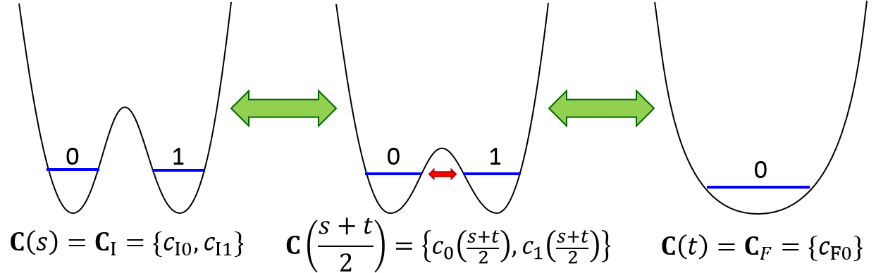
Now, consider what happens if we gradually lower the height of the potential energy barrier. The rate of tunneling and/or thermal excitation over the barrier will increase, and the state will be randomized on ever-shorter timescales. If we continue lowering the barrier to zero height, eventually we will be left with only a single stable ground state of the system. This process corresponds to the process we’ve been describing, of pushing/ejecting a bit of computational information out to the non-computational state of the environment. If the digital state was initially known (correlated with other available information), then it is easy to see that this process results in a net entropy increase of $k\ln 2$ (as in Fig. 9). The process of lowering the barrier can then be reversed, locking the system back into some stable digital state, but the bit value will have become randomized as a result, and our initial knowledge about its value, or any correlations, will be lost—entropy will have increased. However, if the initial digital state was already unknown and uncorrelated, then its state information is already all entropy, and so the process of lowering and re-raising the barrier does not need to increase entropy—in the adiabatic limit (if performed sufficiently slowly), the non-computational entropy does not increase. (But also, computational entropy has not decreased.)

3.4.2 Adiabatic demagnetization.

An example of a very well-studied physical phenomenon that illustrates the connection between information and physics is adiabatic demagnetization, a.k.a. paramagnetic cooling [40, 41, 42]. In this process, used in practice for certain cryogenic refrigeration applications, a magnetic biasing field is gradually removed from a sample of paramagnetic material, which allows the orientations of the magnetic dipoles in the material to randomize themselves. In this process, entropy is transferred from the thermal, kinetic state of the material and its surroundings to the “informational” substrate of the dipole orientations. Since neighboring dipoles tend to align, the dipoles will tend to cluster together into like-aligned domains of some size, which will be relatively stable; these are then very much in the nature of digital bits, and in fact, the information registered in the domains could be utilized in a computational process, as we do in magnetic media, such as disk drives or magnetic memory.

Thus, adiabatic demagnetization is an example of a long-studied physical process by which non-computational entropy (in the kinetic, thermal state of a system) can be transferred to the form of what is effectively digital, computational entropy, and the thermodynamic impact of this transfer of entropy to this more obviously “informational” form is directly measurable. Similarly, the process can be reversed, by gradually applying a field to re-align the dipoles, “erasing” their digital content and thereby heating up their surroundings. The results of all the many decades of laboratory experiments performed on these processes are exactly consistent with standard statistical mechanics, and the entire view of the thermodynamics of computation that we have been discussing.

4 Empirical studies validating Landauer’s Principle

Landauer’s Principle, as explained above, directly and rigorously follows from the enormous and sophisticated success of the theoretical understanding and empirical validation of the concepts of statistical physics that has obtained over the century and a half that have passed since Boltzmann’s pioneering insights. But if any additional assurances are needed, there have been several experiments in recent years that have demonstrated the correctness of Landauer’s Principle more directly. Here we review a few of those experiments, very briefly.

In 2012, Berut et al. [5] tested Landauer’s Principle in the context of a colloidal particle trapped in a modulated double-well potential, an experimental setup designed to mimic the conceptual picture that we reviewed in Fig. 12. Their experimental results showed that the heat dissipated in the erasure operation indeed approached the Landauer value of $k_{\mathrm{B}}T\ln 2$ in the adiabatic limit. Also in 2012, Orlov et al. [6] tested Landauer’s Principle in the context of an adiabatic charge transfer across a resistor, and verified that, in cases where the charge transfer is carried out in a way that does not erase known computational information, the energy dissipated can be much less than $k_{\mathrm{B}}T\ln 2$, which validates the theoretical rationale for doing reversible computing. In 2014, Jun et al. [7] carried an even more high-precision version of the Berut experiment, verifying again the Landauer limit, and that similar, logically-reversible operations can, in contrast, be done in a way that approaches thermodynamic reversibility. Finally, in 2018, Yan et al. [8] carried out a quantum-mechanical experiment demonstrating that Landauer’s Principle holds at the single-atom level.

In contrast, the only experiments that have claimed to demonstrate violations of Landauer’s limit have been ones in which the experimenters misunderstood some basic aspect of the Principle, such as the need to properly generalize the definition of logical reversibility, which was the subject of [11, 12, 13], or the role of correlations that we explained in §3.3 above.

5 Conclusion

In this paper, we reviewed a number of aspects of Landauer’s Principle, including its historical origin in the very foundations of statistical physics, which laid the essential groundwork for modern statistical thermodynamics and quantum mechanics. We saw that information theory is perfectly suited to examining the role of information in physics, and in fact its development historically grew out of statistical physics. Then we detailed exactly how the high-level view of information and computational operations in any real computer connects fundamentally (and unavoidably) with the physical concepts of distinguishable states and bijective dynamics that are essential features of all modern (i.e., quantum) models of fundamental physics. We explained exactly why an irreversible, permanent increase in entropy of $\log 2=k\ln 2$ upon the logically-irreversible, oblivious erasure of a correlated bit is an unavoidable, and totally mathematically rigorous consequence of these fundamental physical theories, and why, in contrast, a reversible computational process can completely avoid the resulting Landauer limit on the energy efficiency of computation, something that traditional computational mechanisms, which discard correlated bits every time a logic gate destructively overwrites its previous output, can never do. Therefore, as reversible computing technologies continue to be improved over time, they can potentially, in the long term, become unboundedly more energy-efficient than all physically possible irreversible computers. Meanwhile, the correctness of Landauer’s Principle, and the fact that only reversible computational processes can circumvent it, have already been directly empirically validated in various experiments.

One caveat to the above statements that could use some further elaboration comes from our observation in §3.3 (also mentioned in [9]) that isolated digital bits that are already entropy (i.e., uncorrelated with any other bits, and unobserved) can be re-randomized, either in-place, such as when the potential barrier is partially lowered in Fig. 12, or by ejecting them to a thermal environment, allowing the environment to randomize them, and subsequently taking them back in, like in adiabatic magnetization/demagnetization, without a necessary increase in total entropy. This raises some potentially interesting algorithmic possibilities for performing randomized computations more energy-efficiently (and securely). For example, cryptographically-secure random bits can be taken in by transferring their entropy adiabatically from a thermal environment, after which a probabilistic algorithm can be executed (reversibly) using those bits, and then (after results are obtained) the utilized entropy can be re-isolated by reversing the computation, after which the random bits used can be pushed back out to the thermal environment, thereby losing them permanently (giving a forward secrecy property) as the environment re-randomizes them, with asymptotically zero net new entropy having been generated in this entire process.

Somewhat more generally, we can also develop a more comprehensive theoretical treatment of the thermodynamics of stochastic computational operations. We could extend the theoretical tools presented in [11, 12, 13] and the present paper, to derive the thermodynamic implications of performing arbitrary, general computational operations in statistical contexts featuring any arbitrary initial probability distributions. This would include stochastic and irreversible operations performed in contexts that exhibit varying degrees of correlation between the part of the state that is being manipulated by the operation, and other parts of the computer. It is conceivable that in the course of undertaking such an investigation, we might uncover a few less-obvious algorithmic opportunities. Developing this more general theory is beyond the scope of the present paper, but would be an appropriate target for future work.

It is hoped that the present paper will help to clarify the fundamental physical justification of Landauer’s Principle. This is especially important since the possibility of approaching reversible computation presents us with the opportunity to eventually make unboundedly-greater gains in the amount of economic value that our civilization may extract in the future from any given energy resources via computation, compared to the best that we could ever accomplish without it. I encourage readers armed with this understanding to invest their own personal energies into helping to develop the reversible computing paradigm towards practical application in the engineering of more efficient computers.

Appendix: Numerical example of the main theorem

In §3.2.4, we described a visualization method to facilitate understanding of the Fundamental Theorem of the Thermodynamics of Computation (eq. 18). The following illustrations (Figs. 13–15) give more detailed numerical values (and some related analytical formulas) for the example summarized in Fig. 3. Note that here, the trees are displayed sideways to save space. Surprisingnesses (horizontal scale) and heavinesses/entropies (proportional to individual/total branch areas) are all dimensioned in units of $k=\log\mathrm{e}$, equivalent to Boltzmann’s constant. The branch thicknesses (vertical scale) are proportional to their (dimensionless) probabilities.

Figure 13: Detailed numerical data for the example of Fig. 3(a), before the grouping operation.

Figure 14: Detailed numerical data for the example of Fig. 3(b), during the grouping operation. In the inset, we also give an analytical derivation showing that the total surprise (length from root to leaf) for each branch is conserved by the grouping operation.

Figure 15: Detailed numerical data for the example of Fig. 3(c), resulting from the grouping operations. The Fundamental Theorem is paraphrased at bottom.

References

- [1] Landauer, R.: Irreversibility and heat generation in the computing process. IBM Journal of Research and Development 5(3), 183–191 (1961). \doi10.1147/rd.53.0183
- [2] Planck, M.: Ueber das Gesetz der Energieverteilung im Normalspectrum. Annalen der Physik 309(3), 553-–563 (1901)
- [3] Bennett, C.H.: Logical reversibility of computation. IBM journal of Research and Development 17(6), 525–532 (1973) \doi10.1147/rd.176.0525
- [4] Lecerf, Y.: Machines de Turing réversibles—Récursive insolubilité en de l’equation , où est un « isomorphisme de codes ». Comptes Rendus Hebdomadaires des Séances de L’académie des Sciences 257, 2597–2600 (1963)
- [5] Bérut, A., Arakelyan, A., Petrosyan, A. Ciliberto, S., Dillenschneider, R., Lutz, E.: Experimental verification of Landauer’s principle linking information and thermodynamics. Nature 483(7388), 187–190 (2012). \doi10.1038/nature10872
- [6] Orlov, A.O., Lent, C.S., Thorpe, C.C., Boechler, G.P., Snider, G.L.: Experimental test of Landauer’s Principle at the sub- level. Japanese Journal of Applied Physics, 51(6S), 06FE10 (2012) \doi10.1143/JJAP.51.06FE10
- [7] Jun, Y., Gavrilov, M., Bechhoefer, J.: High-precision test of Landauer’s principle in a feedback trap. Physical Review Letters 113(19), 190601 (2014). \doi10.1103/PhysRevLett.113.190601
- [8] Yan, L.L., Xiong, T.P., Rehan, K., Zhou, F., Liang, D.F., Chen, L., Zhang, J.Q., Yang, W.L., Ma, Z.H., Feng, M.: Single-Atom Demonstration of the Quantum Landauer Principle. Physical Review Letters 120(21), 210601 (2018). \doi10.1103/PhysRevLett.120.210601
- [9] Frank, M.P.: Approaching the physical limits of computing. In: Proceedings 35th International Symposium on Multiple-Valued Logic (ISMVL 2005), Calgary, Canada, May 2005, pp. 168–-185. IEEE (2005). \doi10.1109/ISMVL.2005.9
- [10] Frank, M.P., DeBenedictis, E.P.: A novel operational paradigm for thermodynamically reversible logic: adiabatic transformation of chaotic nonlinear dynamical circuits. In: IEEE International Conference on Rebooting Computing (ICRC), San Diego, CA, Oct. 2016. IEEE (2016). \doi10.1109/ICRC.2016.7738679
- [11] Frank, M.P.: Foundations of generalized reversible computing. In: Phillips, I., Raham, H. (eds.), Reversible Computation: 9th International Conference, RC 2017, Kolkata, India, July 6-7, 2017, Proceedings, LNCS, vol. 10301, pp. 19–34. Springer, Cham (2017). \doi10.1007/978-3-319-59936-6_2
- [12] Frank, M.P.: Foundations of generalized reversible computing. Extended author’s preprint of [11], https://cfwebprod.sandia.gov/cfdocs/CompResearch/docs/grc-rc17-preprint2.pdf, last accessed 6 June 2018.
- [13] Frank, M.P.: Generalized reversible computing. ArXiv preprint 1806.10183 [cs.ET] (2018)
- [14] Frank, M.P.: Chaotic logic. Presentation, 2016 IEEE International Conference on Rebooting Computing (ICRC), San Diego, CA, Oct. 2016. URL: https://cfwebprod.sandia.gov/cfdocs/CompResearch/docs/Frank_ICRC2016_ChaoticLogic_presUUR+notes.pdf, last accessed 6 June 2018.
- [15] Lent, C.S., Tougaw, P.D., Porod, W.: Quantum cellular automata: the physics of computing with arrays of quantum dot molecules. In: Proceedings, Workshop on Physics of Computation (PhysComp ‘94), Dallas, TX, Nov. 1994. IEEE (1994). \doi10.1109/PHYCMP.1994.363705
- [16] Likharev, K.: Dynamics of some single flux quantum devices: I. Parametric quantron. IEEE Transactions on Magnetics 13(1), 242-–244 (1977). \doi10.1109/TMAG.1977.1059351
- [17] Fredkin, E., Toffoli, T.: Conservative logic. International Journal of Theoretical Physics 21(3–-4), 219-–253 (1982) \doi10.1007/BF01857727
- [18] Drexler, K.E.: Nanosystems: Molecular Machinery, Manufacturing, and Computation. Wiley (1992)
- [19] Younis, S.G., Knight, T.F., Jr.: Practical implementation of charge recovering asymptotically zero power CMOS. In: Borriello, G., Ebeling, C. (eds.) Research in Integrated Systems: Proceedings of the 1993 Symposium, Seattle, WA, Feb. 1993, pp. 234-–250. MIT Press (1993)
- [20] Frank, M.P.: Generalizations of the reversible computing paradigm. Presentation, workshop on “Thermodynamics and Computation: Towards a New Synthesis,” Santa Fe Institute, Aug. 2017. https://cfwebprod.sandia.gov/cfdocs/CompResearch/docs/SFI-talk-final2_ho2up.pdf, last accessed 6 June 2018.
- [21] Frank, M.P.: Generalized reversible computing and the unconventional computing landscape. Presentation, Computer Systems Colloquium, Dept. of EE, Stanford University, Oct. 2017. https://cfwebprod.sandia.gov/cfdocs/CompResearch/docs/Stanford-CS-colloq_v2_ho2up.pdf (slides), https://www.youtube.com/watch?v=IQZ_bQbxSXk (video of presentation), last accessed 6 June 2018.
- [22] Frank, M.P.: The indefinite logarithm, logarithmic units, and the nature of entropy. ArXiv preprint physics/0506128 (2005).
- [23] Frank, M.P.: The physical limits of computing. Computing in Science and Engineering 4(3), 16–26 (2002) \doi10.1109/5992.998637
- [24] Sipser, M.: Introduction to the Theory of Computation, 3rd ed. Cengage Learning (2012)
- [25] Clausius, R.: On the motive power of heat, and on the laws which can be deduced from it for the theory of heat. Poggendorff’s Annalen der Physick, LXXIX (1850).
- [26] Boltzmann, L.: Weitere Studien über das Wärmegleichgewicht unter Gasmolekülen. Sitzungsberichte Akademie der Wissenschaften 66, 275–370 (1872)
- [27] Von Neumann, J.: Thermodynamik quantenmechanischer Gesamtheiten [Thermodynamics of Quantum Mechanical Quantities]. Nachrichten von der Gesellschaft der Wissenschaften zu Göttingen, Mathematisch-Physikalische Klasse 102, 273-–291. (1927)
- [28] Von Neumann, J.: Mathematische Grundlagen der Quantenmechanik. Julius Springer (1932)
- [29] Von Neumann, J.: Mathematical Foundations of Quantum Mechanics. Princeton University Press (1955)
- [30] Shannon, C.E.: A mathematical theory of communication. Bell Systems Technical Journal 27, 379–424 and 623–657 (1948) \doi10.1145/584091.584093
- [31] Shannon, C.E.: The Mathematical Theory of Communication. University of Illinois Press (1949)
- [32] Shannon, C.E.: Communication in the presence of noise. Proceedings of the IRE 37(1), 10–21 (1949)
- [33] Jaynes, E.T.: Information theory and statistical mechanics. Physical review 106(4), 620 (1957)
- [34] Anderson, N.G.: Information erasure in quantum systems. Physics Letters A 372(34), 5552–5555 (2008)
- [35] Anderson, N.G.: Irreversible information loss: Fundamental notions and entropy costs. International Journal of Modern Physics: Conference Series 33, 1460354 (2014) \doi10.1142/S2010194514603548
- [36] Anderson, N.G.: Landauer’s limit and the physicality of information. European Physics Journal B 91, 156 (2018) \doi10.1140/epjb/e2018-80716-6
- [37] Anderson, N.G.: Information as a physical quantity. Information Sciences 415–416, 397–413 (2017) \doi10.1016/j.ins.2017.06.044
- [38] Harada, Y., Goto, E., Miyamoto, N.: Quantum flux parametron. In: 1987 International Electron Devices Meeting, Washington, DC, Dec. 6–9, 1987. IEEE (1987) \doi10.1109/IEDM.1987.191439
- [39] Hosoya, M., Hioe, W., Casas, J., Kamikawai, R., Harada, Y., Wada, Y., Naka ne, H., Suda, R., Goto, E.: Quantum flux parametron—A single quantum flux device for Josephson supercomputer. IEEE Transactions on Applied Superconductivity 1(2), 77–89 (1991) \doi10.1109/77.84613
- [40] De Haas, W.J., Wiersma, E.C., Kramers, H.A.: Experiments on adiabatic cooling of paramagnetic salts in magnetic fields. Physica 1(1–6), 1–13 (1934) \doi10.1016/S0031-8914(34)90002-1
- [41] Kunzler, J.E., Walker, L.R., Galt, J.K.: Adiabatic demagnetization and specific heat in ferrimagnets. Physical Review 119(5), 1609 (1960) \doi10.1103/PhysRev.119.1609
- [42] Pecharsky, V.K., Gschneidner, K.A., Jr.: Magnetocaloric effect and magnetic refrigeration. Journal of Magnetism and Magnetic Materials 200(1–3), 44–56 (1999) \doi10.1016/S0304-8853(99)00397-2