Adversarial Adaptation of Scene Graph Models for Understanding Civic Issues

Abstract.

Citizen engagement and technology usage are two emerging trends driven by smart city initiatives. Governments around the world are adopting technology for faster resolution of civic issues. Typically, citizens report issues, such as broken roads, garbage dumps, etc. through web portals and mobile apps, in order for the government authorities to take appropriate actions. Several mediums – text, image, audio, video – are used to report these issues. Through a user study with 13 citizens and 3 authorities, we found that image is the most preferred medium to report civic issues. However, analyzing civic issue related images is challenging for the authorities as it requires manual effort. Moreover, previous works have been limited to identifying a specific set of issues from images. In this work, given an image, we propose to generate a Civic Issue Graph consisting of a set of objects and the semantic relations between them, which are representative of the underlying civic issue. We also release two multi-modal (text and images) datasets, that can help in further analysis of civic issues from images. We present a novel approach for adversarial training of existing scene graph models that enables the use of scene graphs for new applications in the absence of any labelled training data. We conduct several experiments to analyze the efficacy of our approach, and using human evaluation, we establish the appropriateness of our model at representing different civic issues.

1. Introduction

In recent years, there has been a significant increase in smart city initiatives (Cocchia, 2014; Nam and Pardo, 2011; Neirotti et al., 2014). As a result, government authorities are emphasizing the use of technology and increased citizen participation for better maintenance of urban areas. Various web platforms – SeeClickFix (Mergel, 2012), FixMyStreet (fix, 2016), ichangemycity (IChangeMyCity, 2012) – have been introduced across the world, which enable the citizens to report civic issues such as poor road condition, garbage dumps, missing traffic signs, etc., and track the status of their complaints. Such initiatives have resulted in exponential increase in the number of civic issues being reported (may, 2017). Even social media sites (Twitter, Facebook) have been increasingly utilized to report civic issues. Studies have found the importance of civic issue reporting platforms and social media sites in enhancing civic awareness among citizens (Skoric et al., 2016). These platforms help the concerned authorities to not only identify the problems, but also access the severity of the problems. Civic issues are reported online through various mediums – textual descriptions, images, videos, or a combination of them. Previous work (Dahlgren, 2011) highlights the importance of mediums in citizen participation. Yet, no prior work has tried to understand the role of these mediums in reporting of civic issues.

In this work, we first identify the most preferred medium for reporting civic issues, by conducting a user study with 13 citizens and 3 government authorities. Using the 84 civic issues reported by the citizens using our mobile app, and follow-up semi-structured interviews, we found that images are the most usable medium for the citizens. In contrast, authorities found text as the most preferred medium, as images are hard to analyze at scale.

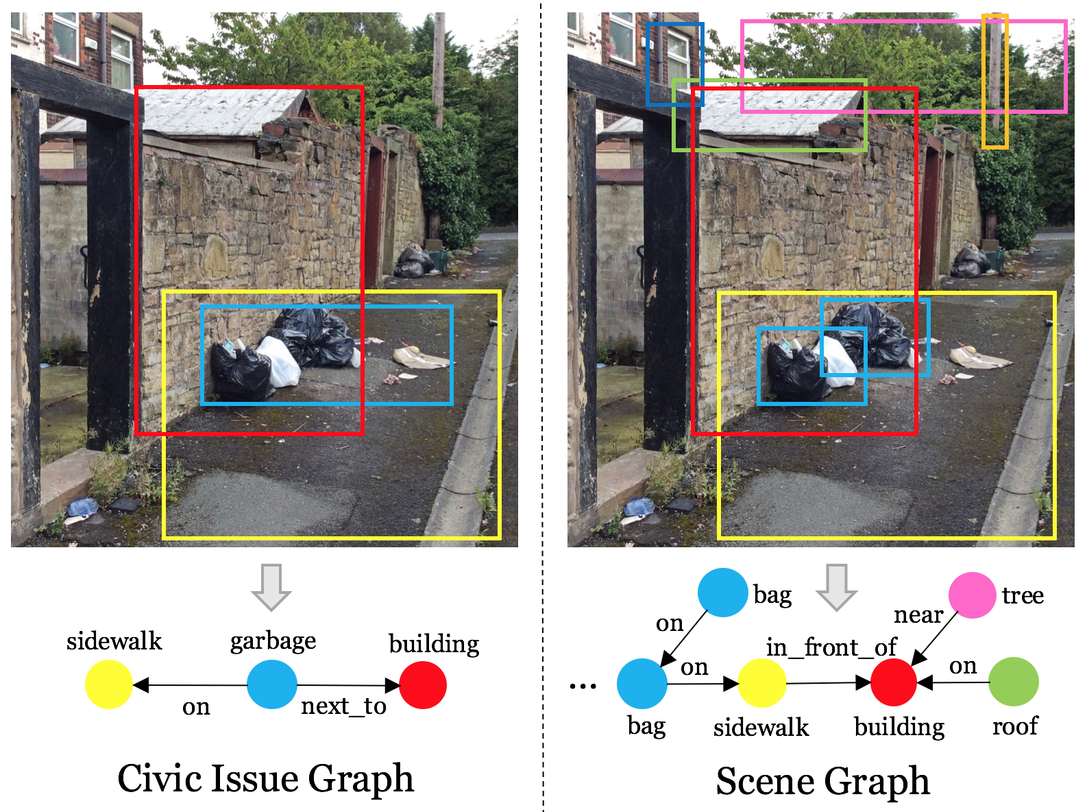
Figure 1. Comparison between Civic Issue Graph and Scene Graph for the same image. The scene graph provides a complete representation of all objects and relationships in the image, while the Civic Issue Graph only consists of relations representative of the civic issue.

To fill this gap, several works have proposed methods to automatically identify a specific category of civic issues from images, such as garbage dumps (Mittal et al., 2016b) and road damage (Maeda et al., 2018). However, their methods are limited to the specific categories that they address. Furthermore, existing holistic approaches of analyzing civic issues are limited to text (Atreja et al., 2018). To this end, we propose an approach to understand various civic issues from input images, independent of the type of issue being reported.

One of the latest advancements in the field of image understanding is generation of scene graphs (Johnson et al., 2015), with the objective of getting a complete structured representation of all objects in an image along with the relations between them. However, to understand a civic issue, only certain crucial objects need to be detected, along with the relations between them, which are representative of the civic issue in the image. Inspired from the task of scene graph generation, we propose to generate Civic Issue Graphs that provide complete representations of civic issues in images.

Figure 1 shows a comparison between the two representations. In contrast to the scene graph, the Civic Issue Graph only consists of objects conveying a civic issue, their bounding boxes, and the predicate between these objects. We present a formal definition of this representation in Section 5.

Training a scene graph model requires a large amount of data consisting of images with grounded annotations (objects and relations in the images). Due to the lack of sufficient annotated images of civic issues, we use an existing scene graph model in a cross-domain setting, with partially annotated and unpaired data. We utilize a dataset extracted by collating and processing public datasets of images from civic issue complaints, for training our model, and make this dataset publicly available. We present a novel adversarial approach that uses an existing scene graph model for a new task in the absence of any labelled training data. To the best of our knowledge, this is the first attempt at adversarial training of an existing scene graph model. We conduct various experiments to establish the efficacy of our approach using metrics derived from standard scene graph evaluation metrics. Finally, through human evaluation, we demonstrate that civic issues from images can be appropriately represented using our Civic Issue Graph.

To summarize, the major contributions of this paper are: (i) understanding the usability of different mediums for reporting civic issues, (ii) introducing a novel unsupervised mechanism using adversarial adaptation of existing scene graph models to a new domain, (iii) experimental evaluation which shows significant performance gains for identification of civic issues from user uploaded images, and (iv) releasing two multi-modal (text and image) datasets with information on civic issues, to encourage future work in this domain.

2. Related Work

Civic Issue Detection and Analysis. Traditionally, different methods have been employed that use technology to gather data about civic issues: such as using laser imaging to identify uneven roads (Eriksson et al., 2008) or gathering data from GPS sensors (Yu and Salari, 2011) for detecting potholes. However, these methods are specific to a particular type of civic issue and require a technological setup with additional costs, which may not be convenient at a larger scale. More recently, social media has provided a convenient interface that allows citizens to report civic issues (Agostino, 2013; Karakiza, 2015). Several works try to analyze online platforms to automatically mine issues related to civic amenities (Mittal et al., 2016a; Mearns et al., 2014), but the analysis is limited to textual descriptions. Specific to images, (Maeda et al., 2018) and (Mittal et al., 2016b) use object detection and image segmentation techniques to identify road damage and garbage dumps respectively, from input images. However, their methods are also limited to the specific category of civic issues that they address. One of the more recent works, ‘Citicafe’ (Atreja et al., 2018) goes a step ahead by allowing users to report various types of civic issues and further employs machine learning techniques to understand and analyze the civic issue from the user input. However, they do not provide a method for understanding images reporting different types of civic issues, as we do in this paper.

Scene-Graph Generation. Several works (Zellers et al., 2018; Klawonn and Heim, 2018) propose methods for generating scene graphs from images to represent all objects in an image and the relationships between them. One approach (Li et al., 2017) includes aligning object, phrase, and caption regions with a dynamic graph based on their spatial and semantic connections. Another approach (Xu et al., 2017) uses standard RNNs and learns to iteratively improve its predictions via message passing. Zellers et al. (Zellers et al., 2018) present a state-of-the-art technique by first establishing that several structural patterns exist in scene-graphs (which they call motifs) and showing how object labels are highly predictive of relation labels by analyzing the Visual Genome dataset (Krishna et al., 2017). All of these approaches require a large set of images for training with grounded annotations for objects and relations. Some works (Zhuang et al., 2018; Liang et al., 2018) utilize zero shot learning for generating a scene-graph. However, their results show that the learning is restricted to the task of detecting new predicates which were not seen during the training phase. Our approach can be used to generalize existing scene graph models to predict new relations belonging to a different domain, which are absent from the training data.

Domain Adaptation. Domain adaptation is a long studied problem, where approaches range from fine-tuning networks with target data (Oquab et al., 2014) to adversarial domain adaptation methods (Tzeng et al., 2017). Some of the deep learning methods propose to learn a latent space that minimizes distance metrics such as maximum mean discrepancy (MMD) (Long et al., 2015) between the source and target domains. A different approach involves domain separation networks which learn to extract image representations that are partitioned into two subspaces: one component which is private to each domain and one which is shared across the two domains (Bousmalis et al., 2016).

The more recently introduced adversarial domain adaptation methods (Tzeng et al., 2017; Ganin and Lempitsky, 2015; Pei et al., 2018) take a different approach by using a domain classifier to learn mappings from the source domain to target domain, which are used to generalize the model to the target domain. Adversarial methods have shown promising results for image understanding tasks such as captioning (Chen et al., 2017a) and object detection (Chen et al., 2018). Hence, in this work, we propose to use Adversarial Discriminative Domain Adaptation (ADDA) (Tzeng et al., 2017) for adapting scene graph models to our new task.

3. User Study

We conducted a user study to understand the preference of different mediums – text, audio, image and video – to report civic issues, both from citizens and authorities perspective. For this, we developed a custom Android app, with the landing page having four buttons, each corresponding to the four mediums. To report an issue, any of the medium(s) could be used any number of times, e.g., a report can comprise of 1 video, few lines of text, and 2 images.

13 participants (9 male, 4 female, age=28.5$\pm$6.1 years) reported civic issues over a period of 7-10 days. All the participants were recruited using word-of-mouth and snowball sampling. All of them were experienced smartphone users, using it for the past 6.2$\pm$2.2 years, and well educated (highest education: 1 high school, 3 Bachelors, 6 Masters, 4 PhDs). However, only two of them have previously reported civic issues on online web portals. At the end of the study, a 30-mins semi-structured interview was conducted, to delve deeper into the reasons for (not) using specific medium(s). Participants were also asked to rate each of the mediums they used on a 5-point Likert scale from NASA-TLX questionnaire (Hart and Staveland, 1988) along with providing subjective feedback. Participants were not compensated for participation.

Furthermore, we interacted with 3 government authorities (3 male, age = 35-45 years) for 30-mins each, to understand their perspective on the medium of the received complaints. All interviews were audio-recorded, and later transcribed for analysis.

3.1. Results

Overall, 84 (6$\pm$3.7) civic issues were reported by the 13 participants, mainly in the category of garbage (11/13 participants), potholes causing water-logging (9), blocked sidewalk (6), traffic (5), illegal car parking (3), and stray dogs (3). 81 of these issues consisted of image, text, or their combination, while only 2 had audio and 1 had video. Hence, here we only focus on image and text as preferred mediums.

A majority of the participants (10/13) found image to be the best medium for reporting civic issues, followed by text (2/13) and video (1/13). Images were preferred mainly because it is quick and easy to click an image, and they convey a lot of information: “An image is worth 1000 words.”-P₄, “its super quick to take pics… even when I pause at a traffic signal, I can take a pic”-P₁₀. Participants also felt that images are best for conveying the severity of a civic problem. They took multiple images from different angles to show the severity of various issues, such as amount of garbage, size of potholes, etc. Interestingly, participants thought that images can “act as a proof of the problem… as images don’t lie”-P₆. On the other hand, participants complained that people might ‘bluff’/‘exaggerate’ when reporting issues using text.

However, participants complained that images can not be used to capture the temporal variations of civic problem, e.g., “images can’t say that this garbage has been here for the past week-P₂. For this, participants favored text medium, as it enables providing details about the temporal variations of an issue. But participants also found that texting requires more time and effort, compared to clicking images.

When participants were asked to choose the best combination of mediums for reporting civic issues, majority of them (9/14) chose image with text. The combination allows them the freedom to show severity and truthfulness of the issue using image, along with adding other details in text. Interestingly when participants were asked to think from the perspective of a government authority, a majority of them (6/13) found text to be the best medium, followed by image (4/13). The main reasons identified by participants were “with huge amounts of data, text is much easier to analyze”-P₇ and at times, images may not be self-explanatory.

Participants’ responses to the 5-point NASA-TLX Likert scale questions for images and text are shown in Figure 2, with the error bars showing the standard deviations. For all metrics, except perceived success, lower score is better. As only a few participants used audio (2/13) and video (3/13), we do not discuss their ratings. A paired t-test showed that images were reported to be significantly better than text, with respect to mental demand (t₁₂=3.56, p¡0.005) and perceived success (t₁₂=2.7, p¡0.01). Only in temporal demand, images performed poorly compared to text, though the difference was not statistically significant. This was because at times participants had to rush/hurry to click the right image.

Following this, we interviewed 3 government authorities, and found about the process of human annotators analyzing the received civic issue image to generate tags and captions describing the issue. These complaint tags are then passed on to the relevant authority in writing or via phone calls to take appropriate actions. Also the authorities confirm that a majority of the received complaints comprise of images. However, these images never reach them due to lack adequate technological infrastructure. This confirms that image is the most preferred medium for users, but authorities rely only on textual complaints. To bridge this gap, in this work, we generate text-based descriptions of images that are used for reporting civic issues.

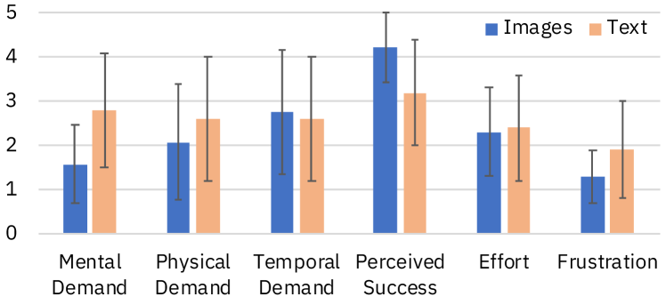
Figure 2. NASA-TLX Likert-scale ratings for Image and Text.

4. Dataset

Object Class	#Images	#Bounding boxes
Garbage	650	831
Manhole	374	419
Pothole	518	677
Water logging	290	375
Total	1505	2302

Table 1. Statistics for Dataset-1

An extensive dataset of images with annotations for a wide variety of civic issues is currently unavailable. To this end, we mined 485,927 complaints (with 131,020 images) from two civic issue reporting forums – FixMyStreet (fix, 2016) and ichangemycity (IChangeMyCity, 2012). We use them to generate two datasets.

Dataset-1 consists of human-annotated images with the bounding boxes and object labels for 4 object categories (Table 1) belonging to the civic issue domain. Some of these object categories are not present in any publicly available image datasets. We utilize the annotations from two existing datasets for garbage (Mittal et al., 2016b) and potholes (Maeda et al., 2018), and add new images representative of the new object categories along with their annotations, to build Dataset-1.

Dataset-2 consists of examples of Civic Issue Graphs, represented through triples of the form $[object1,predicate,object2]$, specifying the relationship ($predicate$) between a pair of objects ($object1$ and $object2$). We use natural language processing techniques (Manning et al., 2014; Schuster et al., 2015) to extract these triples from complaint descriptions. We manually define a set of 19 target object categories which are relevant to the civic domain and map the objects from these triples to our set of target objects using semantic similarity. We retain only those triples where the predicate defines positional relations (manually determined) and for which both objects are matched with a similarity value greater than 0.4. This dataset consists of 44,353 Civic Issue Graphs, where 8204 are paired with images. There are total 5799 unique relations with 19 object classes and 183 predicate classes.

5. Civic Issue Graph Generation

We now present our approach for understanding civic issues from input images. We first present the formal definition of Civic Issue Graphs, followed by our detailed approach, consisting of scene graph generation and adversarial domain adaptation.

Formal Definition: A scene graph is a structured representation of objects and the relationships between them present in an image. It consists of triples or relations (used inter-changeably) of the form $[object1,predicate,object2]$ where $predicate$ defines the relationship between the two objects and both $object1$ and $object2$ are grounded to their respective bounding box representations in the image. While a scene graph provides a complete representation of the contents of the scene in an image, our proposed Civic Issue Graph ($CG$) only consists of objects conveying a civic issue, their bounding boxes, and the predicate between these objects. We use the following notations to define a $CG$:

• $B=\{b_{1},\dots,b_{n}\}$: Set of bounding boxes $b_{i}\in\mathbb{R}^{4}$; $b_{i}$ represents the bounding box for an object $i$, defined as $b_{i}=(x,y,w,h)$, where $x$ and $y$ are co-ordinates of the centre of the bounding box, and $w$ and $h$ are the width and height of the bounding box.

• $O^{1}=\{o^{1}_{1},\dots,o^{1}_{n}\}$: Set of objects essential for defining a civic issue, , e.g., ‘pothole’, ‘garbage’, etc.

• $O^{2}=\{o^{2}_{1},\dots,o^{2}_{n}\}$: Set of objects that define the context of objects in $O^{1}$, e.g., ‘street’, ‘building’, etc.

• $O=O^{1}\cup O^{2}$: Set of all objects that assign a class label $o_{i}\in O$ to each $b_{i}$

• $P=\{p_{1},\dots,p_{n}\}$: Set of predicates defining geometric or position-based relationships between $o^{1}_{i}\in O^{1}$ and $o^{2}_{i}\in O^{2}$, e.g., ‘above’, ‘next_to’, ‘in’, etc.

• $R_{CG}=\{r_{1},\dots,r_{n}\}$: Set of $CG$ relations with nodes $(b_{i},o^{1}_{i})\in B\times O^{1}$, $(b_{j},o^{2}_{j})\in B\times O^{2}$, and predicate label $p_{i\rightarrow j}\in P$, e.g., $[garbage,on,street]$, where $\textit{`garbage'}\in O^{1}$, $\textit{`street'}\in O^{2}$, and $\textit{`on'}\in P$

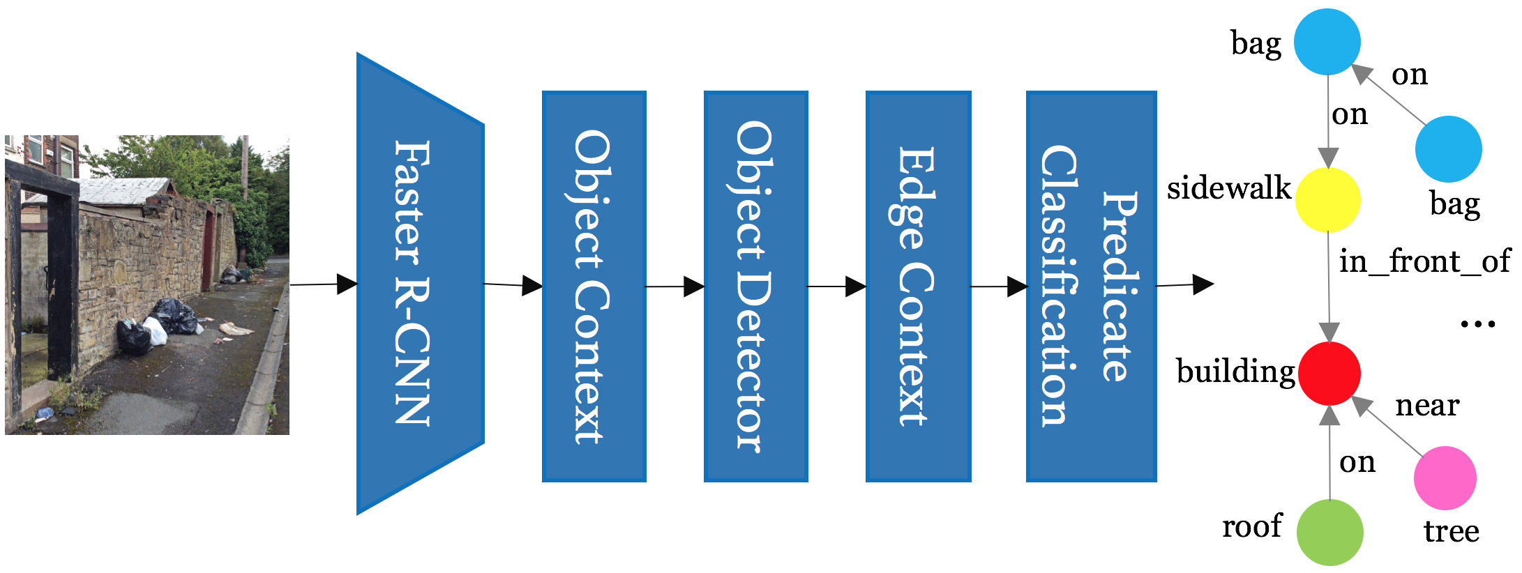
Figure 3. An overview of the MotifNet model

5.1. Scene Graph Generation

Several methods have been proposed for generating scene graphs from images and all of them require labelled training data (Xu et al., 2017; Zellers et al., 2018). The MotifNet model, proposed by Zellers et al. (Zellers et al., 2018), is the current state-of-the-art for generating scene graphs and we utilize this model for demonstrating our approach. However, our approach is generic and can be applied to other models with similar architecture as well.

MotifNet Model: As part of their approach, Zellers et al. highlight that the elements of a visual scene are often governed by the presence of high-level structural regularities, or motifs, such as, “people tend to wear clothes”. Such regularities indicate that given an image – i) predicted object labels may depend on one another, and ii) predicted predicate labels may depend on the predicted object labels. Long Short-Term Memory (LSTM) networks (Hochreiter and Schmidhuber, 1997) are known to capture such dependencies in the input sequence, when the gap between the dependencies is not known. The MotifNet model uses two bidirectional LSTMs (Zhang et al., 2015) to – i) capture the dependencies between object labels (referred as object context), and ii) capture the dependencies between the predicate labels and the object labels (referred as edge context). Fig 3 presents a high-level overview of the model, which consists of:

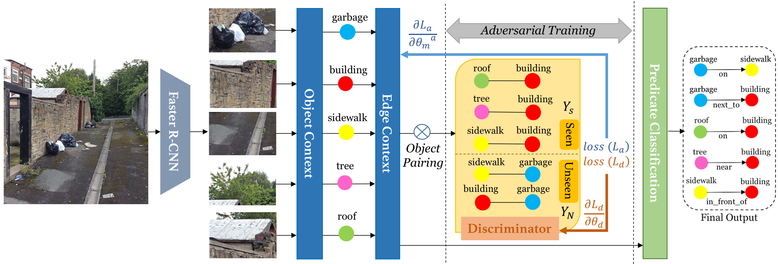
Figure 4. An illustration of our model: Faster R-CNN provides the object labels and their bounding regions. Object context generates a contextualized representation for each object. Edge context generates a contextualized representation for each edge using the representation of the object pairs (head and tail). During adversarial training, information regarding the edge context is passed on to the Discriminator, which learns to distinguish between the $seen$ and $unseen$ object pairs. The training objective of the Discriminator results in gradients flowing into the Discriminator as well as the edge context layer of the MotifNet Model. The loss for the model decreases as the model learns to fool the Discriminator by adapting a uniform representation for $seen$ and $unseen$ classes.

• Object Detection: The MotifNet architecture consists of a Faster R-CNN model (Ren et al., 2015) to detect the objects present in an image. For each image $I$, the object detector provides a set of region proposals, $\mathbf{B}=[\mathbf{b}_{1},\dots,\mathbf{b}_{n}]$. Each region proposal $\mathbf{b}_{i}$, is indicative of an object present in the image and is associated with a feature vector $\mathbf{f}_{i}$ and an object label probability vector $\mathbf{l}_{i}$.

• Object Context: The MotifNet model uses bidirectional LSTM layers to construct a contextualized representation $\mathbf{C}$, for the set of region proposals $\mathbf{B}$. Here $\mathbf{C}$ models the dependencies between different region proposals. Eq. 1 shows the formulation of $\mathbf{C}$, in terms of $\mathbf{f}_{i}$, $\mathbf{l}_{i}$ and $\mathbf{W}_{1}$ where $\mathbf{W}_{1}$ is a parameter matrix that maps $\mathbf{l}_{i}$ to $\mathbb{R}^{100}$.

• Object Decoder: The contextualized representation $\mathbf{C}$, is used to predict the final object labels $\mathbf{O}$. The labels ($\hat{\mathbf{o}}_{i}$) are decoded sequentially using another LSTM, where the hidden state for each label ($\mathbf{h}_{i}$) is conditioned on the previously decoded label (Eq. 2). The hidden state is then used to compute the final object labels $\hat{\mathbf{o}}_{i}$ (Eq. 3).

• Edge Context: The model constructs another contextualized representation $\mathbf{D}$ using additional bidirectional LSTM layers, where $\mathbf{D}$ models the dependency between the relation labels and the object labels . Eq. 4 shows the formulation of $\mathbf{D}$, in terms of $\mathbf{c}_{i}$, $\hat{\mathbf{o}}_{i}$ and $\mathbf{W}_{2}$ where $\mathbf{W}_{2}$ is a parameter matrix that maps $\hat{\mathbf{o}}_{i}$ to $\mathbb{R}^{100}$.

• Predicate Classification: For a sequence of region proposals ($\mathbf{B}$), quadratic number of object pairs are possible. An object pair $(b_{i},b_{j})$, is represented by the model using the final contextualized representations, ($\mathbf{d}_{i},\mathbf{d}_{j}$) and the feature vector ($\mathbf{f}_{i,j}$) representing the union of these objects (Eq. 5). Here $\mathbf{W}_{h},\mathbf{W}_{t}$ project $\mathbf{d}_{i},\mathbf{d}_{j}$ into $\mathbb{R}^{4096}$. The model uses a softmax layer with this representation as input to identify the predicate label ($p_{i\rightarrow j}$) for each object pair or label it as background (Eq. 6). Here, $\mathbf{W}_{t},\mathbf{w}_{o_{i},o_{j}}$ represent the weights of the softmax layer. Object pairs with a valid predicate label (non-background) denote the final relations present in the scene graphs.

Here is the mathematical formulation of the model:

(1) $$\mathbf{C}=[\mathbf{c}_{1},\dots,\mathbf{c}_{n}]=\mathbf{biLSTM({[\mathbf{f}_{i};\mathbf{W}_{1}\mathbf{l}_{i}]}_{i=1,\dots,n})}$$

(2) $$\mathbf{h}_{i}=\mathbf{LSTM}_{i}([\mathbf{c}_{i};\hat{\mathbf{o}}_{i-1}])$$

(3) $$\hat{\mathbf{o}}_{i}=argmax(\mathbf{W}_{o}\mathbf{h}_{i})\>\>|\textrm{one hot vector}|$$

(4) $$\mathbf{D}=[\mathbf{d}_{1},\dots,\mathbf{d}_{n}]=\mathbf{biLSTM}_{i}({[\mathbf{c}_{i};\mathbf{W}_{2}\hat{\mathbf{o}}_{i}]}_{i=1,\dots,n})$$

(5) $$\mathbf{g}_{i,j}=(\mathbf{W}_{h}\mathbf{d}_{i})\circ(\mathbf{W}_{t}\mathbf{d}_{j})\circ\mathbf{f}_{i,j}$$

(6) $$\mathbf{P}(p_{i\rightarrow j}|B,O)=softmax(\mathbf{W}_{r}\mathbf{g}_{i,j}+\mathbf{w}_{o_{i},o_{j}})$$

5.2. Adversarial Domain Adaptation

Domain adaption involves using an existing model trained on “source” domain where labelled data is available, and generalizing it to a “target” domain, where labelled data is not available. Domain adaptation has been helpful for tasks such as image captioning (Chen et al., 2017b) that require a large corpora of images and their labels, as getting this data for each and every domain is unfeasible. More recently, adversarial methods for domain adaptation (Tzeng et al., 2017) have also been proposed, where the training procedure is similar to the training of Generative Adversarial Networks (GANs)(Goodfellow et al., 2014). We present an adversarial training approach for a scene graph model, which, to the best of our knowledge, has not been explored before. Domain adaptation for scene graphs is challenging due to the large domain shift in the images as well as the feature space of relations (Fig. 5). For instance, the Visual Genome dataset (VG) (Krishna et al., 2017) used for training scene graph models, consists of a mix of indoor and outdoor scenes with more object instances, whereas our dataset of civic issues consists of specific outdoor scenes depicting a civic issue. Moreover, some of the relations observed in the civic issue domain are not even present in the visual genome dataset (e.g., garbage-on-street). In the following subsections, we provide more details about our cross-domain setting followed by our approach for adversarial domain adaption.

5.2.1. Cross-Domain Setting

Scene graph models trained on a particular dataset can detect only those relations that are already $seen$ by the model, or in other words, present in the training dataset. For our task of generating $CG$, the model needs to detect ${R}_{CG}$, i.e., the set of relations contained in $CG$. Note that the set of relations in ${R}_{CG}$ can be further divided into ${R}_{s}$ and ${R}_{n}$, where ${R}_{s}$ is the set of relations previously $seen$ by the model, e.g.: $[tree,over,fence]$ and ${R}_{n}$ is the set of relations previously $unseen$ by the model e.g.: $[garbage,on,street]$. In the absence of any labelled data for ${R}_{n}$, we want to generalize the model already trained on ${R}_{s}$, to adapt to ${R}_{n}$ as well.

5.2.2. Adversarial Approach

Adversarial approach for domain adaptation consists of two models – a pre-trained generator model and a discriminator model. In our setting, we use the MotifNet model pre-trained on VG dataset as the generator and propose a discriminator model that can distinguish between ${R}_{s}$ and ${R}_{n}$. During pre-training, the MotifNet model learns a representation for the object pairs (Eq. 5 and 6) which is used to predict the final set of relations (${R}_{s}$). Without adversarial training, the model has not learned the representation for any $unseen$ pair of objects from the civic domain and will not be able to predict such relations (${R}_{n}$). Therefore, during adversarial training, the objective of the MotifNet model is to learn a mapping of target object pairs ($unseen$) to the feature space of the source object pairs ($seen$). This objective is supported via the discriminator, which is a binary classifier between the source and target domains. The MotifNet model can be said to have learned a uniform representation of object pairs corresponding to ${R}_{s}$ and ${R}_{n}$, if the classifier trained using this representation can no longer distinguish between ${R}_{s}$ and ${R}_{n}$. Therefore, we introduce two constrained objectives which seek to – i) find the best discriminator model that can accurately classify ${R}_{s}$ and ${R}_{n}$, and ii) “maximally confuse” the discriminator model by learning new mapping for ${R}_{n}$. Once the source and target feature spaces are regularized, the predicate classifier trained on the $seen$ object pairs can be directly applied to $unseen$ object pairs, thereby eliminating the need for labelled training data.

Fig 4 summarizes our adversarial training procedure. We first pre-train the MotifNet model on the VG dataset using cross-entropy loss and then update it using adversarial training. During adversarial training, the parameters for the MotifNet model and the discriminator are optimised according to a constrained adversarial objective. To optimize the discriminator model, we use the standard classification loss ($L_{d}$). In order to optimize the MotifNet model, we use the standard loss function ($L_{a}$) with inverted labels (seen $\rightarrow$ unseen, unseen $\rightarrow$ seen) thereby satisfying the adversarial objective. This entire training process is similar to the setting of GANs. We iteratively update the MotifNet model and the Discriminator with a ratio of $N_{m}$:$N_{d}$ with $N_{m}<N_{d}$, i.e., the Discriminator is updated more often than the MotifNet model. We now provide a mathematical formulation of our training approach.

Discriminator We define the Discriminator as a binary classifier with $seen$ and $unseen$ as the two set of classes. For each object pair $(o_{i},o_{j})$, the Discriminator is provided with two inputs: 1) $\mathbf{g}_{i,j}$: final representation of the object pair generated by the model and 2) $(\mathbf{W}_{h}\mathbf{d}_{i})\circ(\mathbf{W}_{t}\mathbf{d}_{j})$: contextualized representation of the object pair without the visual features. We further experimented with different inputs to the discriminator (details in Appendix). The Discriminator consists of 2 fully connected layers, followed by a softmax layer to generate probability $C_{d}(l|o_{i},o_{j})$, where $l\in\{seen,unseen\}$. The mathematical formulation of the discriminator for a given object pair ($o_{i}$, $o_{j}$) is:

(7) $$\mathbf{F}_{i,j}=\mathbf{Dis([\mathbf{g}_{i,j};(\mathbf{W}_{h}\mathbf{d}_{i})\circ(\mathbf{W}_{t}\mathbf{d}_{j})])}$$

(8) $$\mathbf{C}_{d}=softmax(\mathbf{W}_{d}\mathbf{F}_{i,j}+\mathbf{b}_{d})$$

Training Discriminator Let ${OP}_{cv}$ be the set of all object pairs identified by the model for an image belonging to the civic domain $\mathbf{I_{cv}}$.

$${OP}_{cv}=MotifNet(\mathbf{I_{cv}})$$

The goal of the Discriminator is formulated as a supervised classification training objective:

(9) $$\mathcal{L}_{d}(\theta_{d})=-\smashoperator[]{\sum_{{OP}_{cv},\>n=1}^{N}}\log\mathbf{C}_{d}(l^{n}|y^{n})$$

$$l^{n}=\left\{\begin{array}[]{ll}1(seen)&\textrm{if }\ y^{n}\in Y_{s}\\[3.0pt] 0(unseen)&\textrm{if }\ y^{n}\in Y_{n},\end{array}\right.$$

where $y^{n}=(o_{i},o_{j})^{n}$, and $Y_{n}$ and $Y_{s}$ are the set of object pairs corresponding to $R_{n}$ and $R_{s}$, respectively. $\theta_{d}$ denotes the parameters of the Discriminator to be learned. We minimize $\mathcal{L}_{d}$ while training the discriminator.

Training Model In accordance with the inverted label loss described above, the training objective of the model is defined as follows:

$$\mathcal{L}_{a}(\theta_{m}^{a})=-\smashoperator[]{\sum_{{OP}_{cv},\>n=1}^{}}^{N}\log\mathbf{C}_{d}(l^{n}|y^{n}) \forall y^{n}\in Y_{n}$$

Here $\theta_{m}^{a}:\{\mathbf{W}_{h},\mathbf{W}_{t}\}$ denotes the parameters of the model that are updated during adversarial training. We minimize $\mathcal{L}_{a}$ while updating the model.

6. Experiments and Evaluation

The simplest approach to identify the civic issue from images is to classify them into a predefined set of categories. We first report the performance of the baseline classifier which categorizes input images into different civic issue categories. The results show the limitations of a classification-based approach for handling images depicting a wide range of civic issues. Following this, we provide the implementation details of our model. We define a set of metrics which are derived from the standard metrics used for scene graph evaluation, for appropriately evaluating our approach. We conduct multiple experiments and provide generic insights for adversarial training of scene graph models. Finally, using human evaluation, we establish the efficacy of our model in appropriately representing civic issues from images.

Classification Approach We trained a classifier (using VGG-16 network pre-trained on MS COCO dataset) to categorize images using the set of ten most frequent categories as defined on FixMyStreet complaint forum (fix, 2016). The classifier was trained on 80640 images and tested using 4992 images.

Category	Test Accuracy
Potholes	82.59
Fly-tipping	81.34
Street/Traffic light	68.37
Graffiti	64.73
Pavements	52.0
Road traffic signs	31.89
Roads	16.42
Garbage	15.59
Drainage/Manhole	7.84
Street Cleaning	4.04

Table 2. Class-wise Accuracy for the classifier

On the test data, this model achieves an accuracy of 47.13%, with F1-score of 38.76. Table 2 shows the class-wise accuracy for the classifier. While the accuracy for the three most accurate classes were 86.5%, 83.6% and 75.2%, 4 out of 10 classes had their accuracy less than 17%. Such large variation in the accuracy for different classes indicates that classifying images into different categories is not sufficient.

6.1. Implementation Details

6.1.1. Data Preprocessing

For all our experiments, we use the datasets defined in Section 4. In order to train the Discriminator, it requires a set of examples corresponding to the two classes: $R_{n}$ and $R_{s}$. Using the dataset-2, we extracted the set of relations ($R_{CG}$) and considered the 150 most frequent triples from this list. We manually refined this set by removing erroneous triples (e.g.: $[pothole,on,building]$) and adding new triples based on existing triples (e.g.: $[garbage,on,sidewalk]\Rightarrow[sidewalk,has,garbage]$). This resulted in 130 triples which are classified as follows: the triples for which the object pair is previously seen by the model, i.e., it is present in the VG dataset, are classified as $R_{s}$ (80 out of 130 triples), and the rest 50 triples are classified as $R_{n}$. For predicate fine-tuning, we use the same set of 130 triples. From dataset-2, we use 90% (7384) of the images for updating the model, and the remaining 820 as test set, which is used for reporting experimental results and for the final human evaluation.

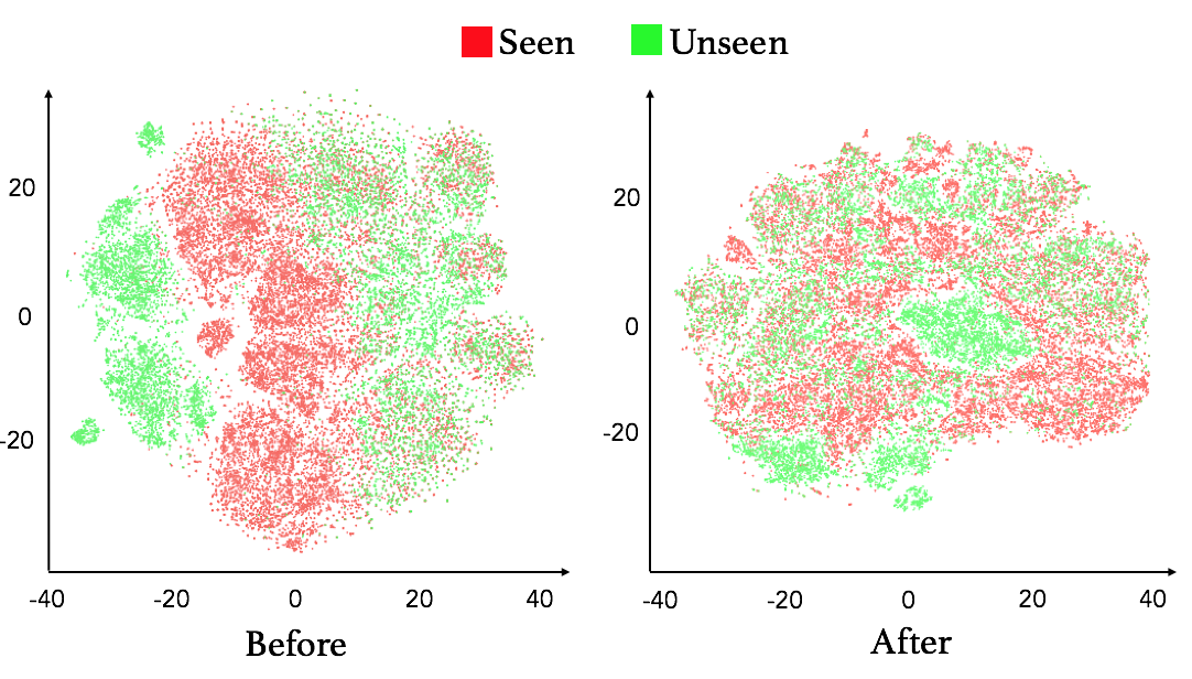
Figure 5. Comparison between the representations (t-SNE embeddings) for $seen$ and $unseen$ object pairs before and after Adversarial Adaptation

6.1.2. Faster R-CNN Training

For the model to detect the objects in the civic domain, we train a Faster R-CNN model for the 19 object classes (present in the Dataset-2). 14 of these classes such as tree, building, street, etc. are already present in VG dataset, and we utilize that for our training. For the remaining 5 classes, such as garbage, pothole, etc., we use the dataset-1. The number of samples of a class from the VG dataset is much higher compared to the number of samples for a class in our new dataset. While training, we ensure an upper limit of 8000 and a lower limit of 3000 on the sample size for each class through a combination of under-sampling and over-sampling. The Faster R-CNN is trained for 10 epochs using SGD optimizer on 3 GPUs, with a batch size of 18 and a learning rate of 1.8 x $10^{-2}$, which was reduced to 1.8 x $10^{-3}$ after validation mAP plateaus.

6.1.3. Scene Graph Model Pre-training

We train the MotifNet model on a subset of VG dataset. We consider the 19 object classes (same as Faster R-CNN) and a (manually) filtered set of 32 predicate classes which are commonly found in the civic domain. We use the Faster R-CNN model trained on the civic domain for object detection. In the final setting, the model is trained without the ‘Object Decoder’ and the difference is highlighted as part of experimental results. The rest of the training setup is same as the original MotifNet model (described in (Zellers et al., 2018)), with the model being trained for 32 epochs. Please see the Appendix more details on pre-training of the MotifNet model.

Figure 6. Qualitative examples presenting the Civic Issue Graphs generated by our model. We show the top 3 relations and highlight the ones that are representative of the civic issue along with their bounding regions

6.1.4. Adversarial Training

Discriminator used in adversarial training consists of 3 fully connected layers: two layers with 4096 hidden units followed by the final softmax output. Each hidden layer is followed by a batch normalization, leakyReLU activation function with negative slope of 0.2 and apply a dropout in the training phase with keeping probability of 0.5. Both discriminator and model are trained using ADAM optimizer with a learning rate of 1.2 x $10^{-2}$ and 1.2 x $10^{-3}$, respectively. The value of $N_{d}$ is set to 150 steps, while $N_{m}$ is set to 50 steps, with the model and the discriminator being trained iteratively for 12 epochs.

6.2. Evaluation Metrics

Previous work (Xu et al., 2017) defines three different modes for analyzing a scene graph model: Predicate Classification (PredCls), Scene Graph Classification (SGCls), and Scene Graph Generation (SGgen). PredCls task examines the performance of the model for detecting the predicate, given a set of object pairs, in isolation from other factors. SGCls task measures the performance of the model for predicting the right object labels and predicates, given a set of localized objects. In SGgen task, the model has to simultaneously detect the set of objects and predict the right predicate for each pair of objects. For our approach of generating Civic Issue Graph ($CG$) using existing scene graph models, it is appropriate to report: (i) the performance of the existing model when generalized to this new domain, and (ii) the accuracy of the output $CG$ for representing the civic issue in the image. Deriving from the existing set of tasks, we define a new set of tasks which can help in evaluating our model along these dimensions:

• OPCls: the task is to predict the set of object pairs which are indicative of the civic issue present in the image.

• CGCls: the task is to predict the set of relations which can represent the civic issue present in the image.

• CGGen: the task is to simultaneously detect the region in the image and predict the right relations which are indicative of the civic issue.

For task OPCls, we report the experimental results, and use human evaluation for the task CGCls and CGGen. In accordance with previous work, for OPCls, we report results for the image-wise recall metrics (R@k). Since our task is to predict object pairs which are found in civic domains, we report results for $R@1$, $R@5$, $R@10$ & $R@20$ metrics. For CGCls and CGGen, we report the results using both Precision and Recall metrics ($k:\{1,3,5\}$)

6.3. Experimental Results

6.3.1. Removing Object Decoder

The MotifNet model after adversarial training performed poorly when tested on the images from civic domain ($R@10=10.5$). We found that the object decoder is not able to predict the correct object labels when the input image contains new objects from the civic domain, as the model has not been trained on these labels. On removing the decoder during test time (denoted as $MotifNet_{Adv}$ in the table), the performance improves significantly ($R@10=76.0$, Table 3). Adapting the decoder to a new domain requires ground-truth data in terms of the sequence of objects and the labels, which may not be possible for the civic domain. Therefore, we decided to pre-train the MotifNet model without the decoder (denoted by $MotifNet^{wd}$) and directly use the object labels predicted by the Faster R-CNN. On updating the new model using adversarial training (denoted by $MotifNet_{Adv}^{wd}$), the performance improved significantly, particularly for $R@1$ and $R@5$. Table 3 shows the comparison between the different settings with $MotifNet_{Adv}^{wd}$ performing significantly better than all other models, for all the metrics.

6.3.2. Adversarial Training vs Fine-tuning

Results from the previous experiment shows that using adversarial training can significantly improve the performance, as the model has now been generalized to both $seen$ and $unseen$ classes. As an alternative approach, we also try to adapt the pre-trained model to our new domain by fine-tuning the predicate classification in the model. Mathematically, we aim to increase the value of $\mathbf{P}(p_{i\rightarrow j}|B,O)$), where $(o_{i},p_{i\rightarrow j},o_{j})$ correspond to $R_{CG}$. The training objective for this phase is defined as:

(10) $$\mathcal{L}_{f}(\theta_{m}^{f})=-\smashoperator[]{\sum_{{OP}_{cv},\>n=1}^{}}^{N}l\log\mathbf{P}(p_{i\rightarrow j}^{n}|B^{n},O^{n})$$

$$l=\left\{\begin{array}[]{ll}1&\textrm{if }\ p_{i\rightarrow j}^{n}\in R_{CG}\\[3.0pt] 0&\textrm{otherwise},\end{array}\right.$$

where $\theta_{m}^{f}:\{\mathbf{W}_{r},\mathbf{w}_{o_{i},o_{j}}\}$, i.e., the weights and bias of the predicate classifier of the model. We minimize $L_{f}$ while fine-tuning the model which is trained for 6 epochs. Table 3 shows that fine-tuning a pre-trained MotifNet model ($MotifNet_{fine}^{wd}$) brings slight improvement in the performance when compared to the original model ($MotifNet$). However, the model with adversarial training ($MotifNet_{Adv}^{wd}$) performs significantly better than the fine-tuned model ($MotifNet_{fine}^{wd}$). Fine-tuning the model will only improve the detection of relations which are already $seen$ by the model, while adversarial training will generalize the performance across both $seen$ and $unseen$ classes. This is further highlighted in Fig. 5 that shows how the difference between the representations of $seen$ and $unseen$ relations has reduced through adversarial training. Further fine-tuning the adversarially updated MotifNet ($MotifNet_{Adv+fine}^{{wd}}$) model brings no improvement in the performance.

Model Settings	R@1	R@5	R@10	R@20
$MotifNet$	35.6	64.9	75.4	79.7
$MotifNet_{Adv}$	37.7	65.7	76.0	79.8
$MotifNet^{wd}$	37.7	63.0	73.3	78.9
$MotifNet^{wd}_{Adv}$	43.3	67.7	76.3	80.2
$MotifNet_{fine}^{wd}$	38.9	63.6	73.8	79.2
$MotifNet_{Adv+fine}^{wd}$	43.1	67.7	76.3	80.2

Table 3. Recall for different settings; ${Adv}$: Adversarial Training; $fine$: fine-tuning; ${wd}$: without decoder setting

6.4. Human Evaluation

To establish the efficacy of our model at appropriately representing civic issues from images, we asked Amazon Mechanical Turk workers to evaluate the output of our model. We randomly sampled 300 images from the test set; each image was evaluated by 3 workers. In accordance with our definition of $CG$, we filtered the final set of relations generated by our model and kept only the top 5 relations for which $o_{i}\in O_{1}$ and $o_{j}\in O_{2}$ where $(o_{i},o_{j})$ denotes the unordered set of objects in a relation (refer Section LABEL:formaldef).

The evaluation was carried out for the two tasks – CGCls and CGGen in two phases. For the task CGCls, workers were shown an image along with 5 relations and were asked to select 0 or more relations that appropriately represent the civic issue(s) in that image along with an option to specify any additional relations separately. For the task CGGen, we retrieved the set of relations which were marked as relevant for a given image. For each such relation, the workers were shown the bounding regions for the objects present in the relation, and asked to evaluate the coverage of these bounding regions, on a scale of 0 to 10. We report two metrics – Precision and Recall, for both the tasks and consider only the majority voted relations with a minimum average rating of 5 for the bounding regions. Table 4 shows the performance of our model. The results show that 83.3% of the times, the relation representing a civic issue is present in the top 3 relations of our $CG$, and 53.0% of the times, the top relation itself represents a civic issue in the image. The accuracy on the CGGen task further indicates that our model is capable of generating accurate groundings for the objects representing the civic issue.

	CGCls			CGGen
	@1	@3	@5	@1	@3	@5
Precision	53.0	31.9	24.7	50.9	30.3	24.1
Recall	53.0	84.0	99.0	50.9	83.3	99.0

Table 4. Precision and Recall values for the tasks CGCls and CGGen based on human evaluation

7. Discussion

The approach we presented in this paper can be utilized in existing platforms, which allow users to report civic issues using images. Once the user uploads an image, our model can automatically generate text-based relations (e.g., garbage-on-street, garbage-next to-building) depicting the civic issue in the input image. These text-based relational descriptions can be shared with the authorities, which can be utilized for large scale analysis, thereby automating the process and removing any dependency on the actual image uploaded by the user. Furthermore, if needed, natural language descriptions can be generated from these relations using a template-based approach. If the confidence of our model is low, the user can be asked to verify the output generated by the model, before sending it to the authorities. Data collected in this process can be further used for retraining the model to improve its performance.
Limitations: While our model can understand a wide range of civic issues from images, some issue categories either cannot be captured using images or require additional information in text to adequately report the issue. For example, irregular water supply problem, car speeding on the road, etc. requires text to report the number of days of irregular water supply or the car number plate details.

The importance of scene graph representation of images has already been proven for several tasks, including semantic image retrieval (Johnson et al., 2015) and visual question answering (Krishna et al., 2017). However, previous approaches rely on extensive ground truth annotations to train the scene graph model. This has limited the scope of scene graphs in domains where obtaining such annotated data is either unfeasible or costly. For instance, in the education domain, the semantic understanding of an image through a scene graph representation (e.g., bat-has-wings, bat-inside-cave) can support learning through automatic generation of picture stories and image-based assessments. In the fashion domain, scene graphs can be used to create ontologies with objects such as accessories, clothes, and more. Even though we present a specific application of generating Civic Issue Graphs, our presented approach and the insights gained from our experiments can help expand the generation of scene graphs for other domains as well, by reducing the dependency on extensive ground truth annotations.

8. Conclusion

We introduce a novel unsupervised mechanism of adapting existing scene graph models via adversarial training and present an application of our approach for generating Civic Issue Graph. The Civic Issue Graph can provide a complete representation for images with different types of civic issues, to help bridge the gap between images and text descriptions used to report issues. Our experimental analysis helps provide a framework for adapting scene graph models to other settings as well. We also release two multi-modal (text and images) datasets with information of civic issues, to encourage future work in this domain.

Appendix A Appendix

A.1. MotifNet Model

We use 32 predicates classes and 19 object classes to train the MotifNet model on a subset of Visual Genome dataset. Table  5 and  6 show the frequencies of objects and predicates used for the training of MotifNet model.

Object	Frequency	Object	Frequency
animal	3611	bag	7391
bottle	6246	box	5467
building	31805	car	17352
fence	12027	house	5006
letter	6630	pole	21205
sidewalk	9478	sign	23499
street	10996	tree	49902
crack	1313	garbage	217
pothole	19	manhole	179

Table 5. Object Frequency for training MotifNet

Predicate	Frequency	Predicate	Frequency
above	47341	across	1996
against	3092	along	3624
at	9903	attached to	10190
behind	41356	between	3411
carrying	5213	covered in	2312
covering	3806	flying in	1973
from	2945	growing on	1853
hanging from	9894	has	277936
in	251756	in front of	13715
laying on	3739	lying on	1869
mounted on	2253	near	96589
on	712409	on back of	1914
over	9317	painted on	3095
parked on	2721	part of	2065
sitting on	18643	standing on	14185
under	22596	with	66425

Table 6. Predicate Frequency for training MotifNet

We trained 2 variants of MotifNet model: with object decoder and without object decoder. Table  7 shows the evaluation of both the models on the VG dataset.

Model	R@20	R@50	R@100
$MotifNet-VG$	24.56	28.08	30.18
$MotifNet^{wd}-VG$	22.49	26.58	28..35

Table 7. MotifNet model Results on Visual Genome dataset

A.2. Classification

Table 8 highlights the confusion between the different classes of the classifier. The confusion occurs mostly because the images describing different types of civic issues can have very similar visual features (e.g. Roads and Potholes) and some categories of issues only differ in their semantic interpretation (e.g. Garbage and Fly-tipping). Despite the similarities, it is still important to maintain this distinction in order to understand the nature of civic issues. Different categories often have different resolution process and may involve different authorities.

True Class	Predicted Class (%)
$C_{1}$: Potholes	$C_{1}$, 86.5	$C_{6}$, 4.9	$C_{4}$, 4.2
$C_{2}$: Street light	$C_{2}$, 75.2	$C_{3}$, 6.4	$C_{7}$, 5.9
$C_{3}$: Fly-tipping	$C_{3}$, 83.6	$C_{6}$, 4.9	$C_{5}$, 4.5
$C_{4}$: Roads	$\mathbf{C_{1}}$, 39.7	$C_{4}$, 20.7	$\mathbf{C_{6}}$, 18.2
$C_{5}$: Garbage	$\mathbf{C_{3}}$, 57.8	$C_{5}$, 25.3	$C_{6}$, 7.6
$C_{6}$: Pavements	$C_{6}$, 53.6	$C_{1}$, 19.5	$C_{3}$, 14.2
$C_{7}$: Road signs	$C_{7}$, 37.2	$C_{2}$, 17.6	$C_{3}$, 6.0
$C_{8}$: Drainage	$\mathbf{C_{1}}$, 30.3	$\mathbf{C_{6}}$, 20.4	$C_{4}$, 16.5
$C_{9}$: Street cleaning	$\mathbf{C_{3}}$, 33.4	$\mathbf{C_{6}}$, 23.5	$C_{1}$, 15.5

Table 8. Top three predictions per class, representing the confusion matrix

A.3. Changing the input of the Discriminator

While updating the model using adversarial training (denoted by $MotifNet_{Adv}^{wd}$) the input to the discriminator is: $[\mathbf{g}_{i,j};(\mathbf{W}_{h}\mathbf{d}_{i})\circ(\mathbf{W}_{t}\mathbf{d}_{j})]$ as mentioned in the paper. Here, $(\mathbf{W}_{h}\mathbf{d}_{i})\circ(\mathbf{W}_{t}\mathbf{d}_{j})$ denotes the contextualized representation of an object pair $\mathbf{(o_{i},o_{j})}$ generated by the model. We also tested the model using another input for the discriminator: $\mathbf{g}_{i,j}$, which is a dot product of the contextualized representation $((\mathbf{W}_{h}\mathbf{d}_{i})\circ(\mathbf{W}_{t}\mathbf{d}_{j}))$ and the visual features $(f_{i,j})$ for the object pairs. However, in the second case, with $\mathbf{g}_{i,j}$ as the input (denoted by $MotifNet_{Adv}^{wd*}$, Table  9) the improvements in the score were much less.

Model Settings	R@1	R@5	R@10	R@20
$MotifNet_{Adv}^{wd}$	43.3	67.7	76.3	80.2
$MotifNet_{Adv}^{wd*}$	38	63.1	73.3	79.2

Table 9. Recall for different inputs to the Discriminator; $\mathbf{Adv}$ denotes Adversarial Training, $*$ denotes the setting with $\mathbf{g}_{i,j}$ as input, and $wd$ denotes without decoder setting

References

- (1)
- fix (2016) 2016. FixMyStreet. (2016). https://www.fixmystreet.com/
- may (2017) 2017. Mayor’s Management Report. https://www1.nyc.gov/assets/operations/downloads/pdf/mmr2017/2017_mmr.pdf. (2017).
- Agostino (2013) Deborah Agostino. 2013. Using social media to engage citizens: A study of Italian municipalities. Public Relations Review 39, 3 (2013), 232–234.
- Atreja et al. (2018) Shubham Atreja, Pooja Aggarwal, Prateeti Mohapatra, Amol Dumrewal, Anwesh Basu, and Gargi B Dasgupta. 2018. Citicafe: An Interactive Interface for Citizen Engagement. In 23rd International Conference on Intelligent User Interfaces. ACM, 617–628.
- Bousmalis et al. (2016) Konstantinos Bousmalis, George Trigeorgis, Nathan Silberman, Dilip Krishnan, and Dumitru Erhan. 2016. Domain separation networks. In Advances in Neural Information Processing Systems. 343–351.
- Chen et al. (2017a) Tseng-Hung Chen, Yuan-Hong Liao, Ching-Yao Chuang, Wan Ting Hsu, Jianlong Fu, and Min Sun. 2017a. Show, Adapt and Tell: Adversarial Training of Cross-Domain Image Captioner.. In ICCV. 521–530.
- Chen et al. (2017b) Tseng-Hung Chen, Yuan-Hong Liao, Ching-Yao Chuang, Wan Ting Hsu, Jianlong Fu, and Min Sun. 2017b. Show, Adapt and Tell: Adversarial Training of Cross-Domain Image Captioner.. In ICCV. 521–530.
- Chen et al. (2018) Yuhua Chen, Wen Li, Christos Sakaridis, Dengxin Dai, and Luc Van Gool. 2018. Domain Adaptive Faster R-CNN for Object Detection in the Wild. In Computer Vision and Pattern Recognition (CVPR).
- Cocchia (2014) Annalisa Cocchia. 2014. Smart and digital city: A systematic literature review. In Smart city. Springer, 13–43.
- Dahlgren (2011) Peter Dahlgren. 2011. Parameters of online participation: Conceptualising civic contingencies. Communication management quarterly 21, 4 (2011), 87–110.
- Eriksson et al. (2008) Jakob Eriksson, Lewis Girod, Bret Hull, Ryan Newton, Samuel Madden, and Hari Balakrishnan. 2008. The pothole patrol: using a mobile sensor network for road surface monitoring. In Proceedings of the 6th international conference on Mobile systems, applications, and services. ACM, 29–39.
- Ganin and Lempitsky (2015) Yaroslav Ganin and Victor Lempitsky. 2015. Unsupervised Domain Adaptation by Backpropagation. In Proceedings of the 32Nd International Conference on International Conference on Machine Learning - Volume 37 (ICML’15). JMLR.org, 1180–1189. http://dl.acm.org/citation.cfm?id=3045118.3045244
- Goodfellow et al. (2014) Ian Goodfellow, Jean Pouget-Abadie, Mehdi Mirza, Bing Xu, David Warde-Farley, Sherjil Ozair, Aaron Courville, and Yoshua Bengio. 2014. Generative Adversarial Nets. In Advances in Neural Information Processing Systems 27, Z. Ghahramani, M. Welling, C. Cortes, N. D. Lawrence, and K. Q. Weinberger (Eds.). Curran Associates, Inc., 2672–2680. http://papers.nips.cc/paper/5423-generative-adversarial-nets.pdf
- Hart and Staveland (1988) Sandra G Hart and Lowell E Staveland. 1988. Development of NASA-TLX (Task Load Index): Results of empirical and theoretical research. Advances in psychology 52 (1988), 139–183.
- Hochreiter and Schmidhuber (1997) Sepp Hochreiter and Jürgen Schmidhuber. 1997. Long short-term memory. Neural computation 9, 8 (1997), 1735–1780.
- IChangeMyCity (2012) IChangeMyCity. 2012. https://ichangemycity.com. (2012).
- Johnson et al. (2015) Justin Johnson, Ranjay Krishna, Michael Stark, Li-Jia Li, David Shamma, Michael Bernstein, and Li Fei-Fei. 2015. Image retrieval using scene graphs. In Proceedings of the IEEE conference on computer vision and pattern recognition. 3668–3678.
- Karakiza (2015) Maria Karakiza. 2015. The impact of social media in the public sector. Procedia-Social and Behavioral Sciences 175 (2015), 384–392.
- Klawonn and Heim (2018) Matthew Klawonn and Eric Heim. 2018. Generating Triples with Adversarial Networks for Scene Graph Construction. arXiv preprint arXiv:1802.02598 (2018).
- Krishna et al. (2017) Ranjay Krishna, Yuke Zhu, Oliver Groth, Justin Johnson, Kenji Hata, Joshua Kravitz, Stephanie Chen, Yannis Kalantidis, Li-Jia Li, David A Shamma, and others. 2017. Visual genome: Connecting language and vision using crowdsourced dense image annotations. International Journal of Computer Vision 123, 1 (2017), 32–73.
- Li et al. (2017) Yikang Li, Wanli Ouyang, Bolei Zhou, Kun Wang, and Xiaogang Wang. 2017. Scene graph generation from objects, phrases and region captions. In Proceedings of the IEEE Conference on Computer Vision and Pattern Recognition. 1261–1270.
- Liang et al. (2018) Kongming Liang, Yuhong Guo, Hong Chang, and Xilin Chen. 2018. Visual Relationship Detection with Deep Structural Ranking. (2018).
- Long et al. (2015) Mingsheng Long, Yue Cao, Jianmin Wang, and Michael I Jordan. 2015. Learning transferable features with deep adaptation networks. arXiv preprint arXiv:1502.02791 (2015).
- Maeda et al. (2018) Hiroya Maeda, Yoshihide Sekimoto, Toshikazu Seto, Takehiro Kashiyama, and Hiroshi Omata. 2018. Road Damage Detection Using Deep Neural Networks with Images Captured Through a Smartphone. arXiv preprint arXiv:1801.09454 (2018).
- Manning et al. (2014) Christopher Manning, Mihai Surdeanu, John Bauer, Jenny Finkel, Steven Bethard, and David McClosky. 2014. The Stanford CoreNLP natural language processing toolkit. In Proceedings of 52nd annual meeting of the association for computational linguistics: system demonstrations. 55–60.
- Mearns et al. (2014) Graeme Mearns, Rebecca Simmonds, Ranald Richardson, Mark Turner, Paul Watson, and Paolo Missier. 2014. Tweet my street: a cross-disciplinary collaboration for the analysis of local twitter data. Future Internet 6, 2 (2014), 378–396.
- Mergel (2012) Ines Mergel. 2012. Distributed democracy: Seeclickfix. com for crowdsourced issue reporting. (2012).
- Mittal et al. (2016b) Gaurav Mittal, Kaushal B Yagnik, Mohit Garg, and Narayanan C Krishnan. 2016b. Spotgarbage: smartphone app to detect garbage using deep learning. In Proceedings of the 2016 ACM International Joint Conference on Pervasive and Ubiquitous Computing. ACM, 940–945.
- Mittal et al. (2016a) Nitish Mittal, Swati Agarwal, and Ashish Sureka. 2016a. Got a Complaint?-Keep Calm and Tweet It!. In International Conference on Advanced Data Mining and Applications. Springer, 619–635.
- Nam and Pardo (2011) Taewoo Nam and Theresa A Pardo. 2011. Conceptualizing smart city with dimensions of technology, people, and institutions. In Proceedings of the 12th annual international digital government research conference: digital government innovation in challenging times. ACM, 282–291.
- Neirotti et al. (2014) Paolo Neirotti, Alberto De Marco, Anna Corinna Cagliano, Giulio Mangano, and Francesco Scorrano. 2014. Current trends in Smart City initiatives: Some stylised facts. Cities 38 (2014), 25–36.
- Oquab et al. (2014) Maxime Oquab, Leon Bottou, Ivan Laptev, and Josef Sivic. 2014. Learning and transferring mid-level image representations using convolutional neural networks. In Proceedings of the IEEE conference on computer vision and pattern recognition. 1717–1724.
- Pei et al. (2018) Zhongyi Pei, Zhangjie Cao, Mingsheng Long, and Jianmin Wang. 2018. Multi-Adversarial Domain Adaptation. In AAAI.
- Ren et al. (2015) Shaoqing Ren, Kaiming He, Ross Girshick, and Jian Sun. 2015. Faster r-cnn: Towards real-time object detection with region proposal networks. In Advances in neural information processing systems. 91–99.
- Schuster et al. (2015) Sebastian Schuster, Ranjay Krishna, Angel Chang, Li Fei-Fei, and Christopher D Manning. 2015. Generating semantically precise scene graphs from textual descriptions for improved image retrieval. In Proceedings of the fourth workshop on vision and language. 70–80.
- Skoric et al. (2016) Marko M Skoric, Qinfeng Zhu, Debbie Goh, and Natalie Pang. 2016. Social media and citizen engagement: A meta-analytic review. New Media & Society 18, 9 (2016), 1817–1839.
- Tzeng et al. (2017) Eric Tzeng, Judy Hoffman, Kate Saenko, and Trevor Darrell. 2017. Adversarial discriminative domain adaptation. In Computer Vision and Pattern Recognition (CVPR), Vol. 1. 4.
- Xu et al. (2017) Danfei Xu, Yuke Zhu, Christopher B Choy, and Li Fei-Fei. 2017. Scene graph generation by iterative message passing. In Proceedings of the IEEE Conference on Computer Vision and Pattern Recognition, Vol. 2.
- Yu and Salari (2011) X Yu and E Salari. 2011. Pavement pothole detection and severity measurement using laser imaging. In Electro/Information Technology (EIT), 2011 IEEE International Conference on. IEEE, 1–5.
- Zellers et al. (2018) Rowan Zellers, Mark Yatskar, Sam Thomson, and Yejin Choi. 2018. Neural Motifs: Scene Graph Parsing with Global Context. In Proceedings of the IEEE Conference on Computer Vision and Pattern Recognition. 5831–5840.
- Zhang et al. (2015) Shu Zhang, Dequan Zheng, Xinchen Hu, and Ming Yang. 2015. Bidirectional long short-term memory networks for relation classification. In Proceedings of the 29th Pacific Asia Conference on Language, Information and Computation. 73–78.
- Zhuang et al. (2018) Bohan Zhuang, Qi Wu, Chunhua Shen, Ian D Reid, and Anton van den Hengel. 2018. HCVRD: A Benchmark for Large-Scale Human-Centered Visual Relationship Detection.. In AAAI.