Optimal uni-axial ferromagnetism in (La,Ce)₂Fe₁₄B for permanent magnets

Abstract

Prospects for light-rare-earth-based permanent magnet compound R₂Fe₁₄B (R=La_1-xCe_x with $0\leq x\leq 1$) are inspected from first principles referring to the latest experimental data. Ce-rich 2:14:1 compounds come with good structure stability, reasonably good combination of magnetization and magnetic anisotropy, while a drawback lies in the low Curie temperature that is only 120 K above the room temperature at the Ce₂Fe₁₄B limit. Best compromise is inspected on the basis of ab initio data for (La_1-xCe_x)₂Fe₁₄B referring to the magnetic properties of the champion magnet compound Nd₂Fe₁₄B and prerequisite conditions imposed by practical utility.

I Introduction

Rare-earth permanent magnets make one of the most important materials in the upcoming decades with expectedly extensive industrial applications in electric vehicles and robotics. Permanent magnets exploit a metastable state in the magnetization curve of uni-axial ferromagnets. Strong magnetization and high Curie temperature can be basically achieved with Fe-based ferromagnets which can be supplemented with rare metals like Nd and Co to get a good combination of uni-axial magnetic anisotropy and even higher Curie temperature, respectively. Today’s commercial champion magnet is made of Nd₂Fe₁₄B sagawa_1984 ; croat_1984 ; rmp_1991 . The problem with this material sometimes happens with relatively low Curie temperature at 585 K. Addition of Co or Dy has been a practical solution to supplement high-temperature performance and recent developments have been concentrated on finding a way to reduce the amount of such expensive elements. Even Nd might face a short supply in the upcoming few decades and we are motivated to find a way to reduce the amount of Nd. Thus the target compound in the present study is (La_1-xCe_x)₂Fe₁₄B with $0\leq x\leq 1$ with the cheap light rare earth elements, La and Ce, as a possible replacement for Nd₂Fe₁₄B.

We address the intrinsic magnetic properties of (La_1-xCe_x)₂Fe₁₄B from first principles as a complementary approach to the recent experimental study apl_2016 and estimate the merit of the compound as a function of $x$ referring to the intrinsic properties of Nd₂Fe₁₄B. Addition of Co is excluded here in order to elucidate the $4f$-electron physics in La_1-xCe_x keeping the rest simple by restricting the scope of the $3d$-electron part only to Fe. Conventional prospect for Ce in the permanent magnet community seems to have been bad because Ce is typically detrimental to Curie temperature and hardly contributes to magnetization. We identify other utility of Ce in the structure stabilization and possibly also in the volume effect. We will also see that magnetic anisotropy coming from Ce can be superior to that from $3d$-electrons, if not on a par with Nd anisotropy. Furthermore, exceptionally high Curie temperature in Ce-based ferromagnet has been known in CeRh₃B₂ whose Curie temperature at 125 K is higher than its Gd counterpart at 90 K cerh3b2 . These point to the possibility for more exploitation of subtlety in the interplay between $f$-electrons and $d$-electrons in Ce-based intermetallics for permanent magnets.

The rest of this paper is organized as follows. In the next section we describe our ab initio methods. In Sec. III calculated results for formation energy, magnetization, magnetic anisotropy, and Curie temperature are presented and the merit associated with them are estimated. In Sec. IV some subtle points in the utility of Ce are discussed. The last section is devoted for conclusions and outlook.

II Methods

Intrinsic magnetic properties of (La_1-xCe_x)₂Fe₁₄B with $0\leq x\leq 1$ are calculated from first principles combining two approaches. One is ab initio structure optimization utilizing the open-source software package OpenMX OpenMX ; Ozaki2003 ; Ozaki2004 ; Ozaki2005 ; Duy2014 ; Lejaeghere2016 on the basis of pseudopotentials MBK1993 ; Theurich2001 and local orbital basis sets. This aproach is attempted at the stoichiometric limits, $x=0$ and $x=1$, and also for chemical compositions where discrete replacement is doable in the unit cell, i.e. $x=n/8$ with $n=1,2,\ldots,7$, out of the eight rare-earth atomic sites in the unit cell of 2:14:1 crystal structure rmp_1991 . The other is Korringa-Kohn-Rostoker (KKR) korringa ; kohn Green’s function approach incorporating coherent potential approximation (CPA) shiba_akai as implemented in the package AkaiKKR AkaiKKR . With KKR-CPA, replacements between La and Ce can be explored continuously on the chemical composition axis. The experimentally inspected mixing ratio and the particular sublattice preference of Ce in La apl_2016 can be continuously simulated as well.

II.1 Discrete and continous interpolation ab initio between La₂Fe₁₄B and Ce₂Fe₁₄B

II.1.1 Ab initio structure optimization: the discrete way

In ab initio electronic structure calculations based on density functional theory hohenberg_1964 ; kohn_1965 , it has been known that the lattice structure of Fe-based ferromagnets seems to be best described within Generalized Gradient Approximation (GGA) as proposed Perdew, Burke, and Ernzerhof (PBE) prl_1996 . We do ab initio structure optimization for (La,Ce)₂Fe₁₄B to track the trend of formation energy from La₂Fe₁₄B to Ce₂Fe₁₄B. The basis set we take in OpenMX is Ce8.0-s2p2d2f1, La8.0-s2p2d2f1, Fe6.0S-s2p2d1, and B7.0-s3p3d2 within the given pseudopotential data set OpenMX . In the discussions below Y₂Fe₁₄B is sometimes taken as a $3d$-electron analogue for the reference to elucidate the contribution from $4f$-electron part in La_1-xCe_x. For that case the basis Y8.0-s3p2d2f1 is used for Y₂Fe₁₄B. The energy cutoff is set to be 500 Ry which was tuned together with the choice of the basis sets to ensure the convergence. Too rich basis set can trigger instability the calculated results presumably due to overcompleteness of the basis Ozaki2004 and we did not quite achieve the convergence with richer basis sets like Ce8.0-s3p3d3f2 in the given pseudopotential data set OpenMX for this particular case of Ce₂Fe₁₄B. For the present purpose to systematically track the trends between La₂Fe₁₄B to Ce₂Fe₁₄B, we settled down with the basis set Ce8.0-s2p2d2f1. Similar basis sets with a little more or less inclusion of local basis wavefunctions can be good as well depending on the target materials and the issue being investigated as long as the choice of the basis set is coherently applied to the target materials and the reference materials.

Number of k points is set to be $64$ for the 2:14:1 materials. For Ce₂Fe₁₄B, more extensive runs with k-point number being up to $256$ were verified as well and we have seen that sufficient convergence has been achieved already at the stage where the k point number is $64$.

The starting structure is taken from the experimental measurements rmp_1991 ; apl_2016 and ab initio structure optimization is done for (La_1-xCe_x)₂Fe₁₄B with $x=n/8$ where $n=0,1,2,\ldots,8$ to get the minimized energy $U_{\rm tot}[\mbox{(La${}_{1-x}$Ce${}_{x}$)${}_{2}$Fe${}_{14}$B}]$ and the associated magnetization in the ground state. The structure optimization is done allowing for magnetic polarization without spin-orbit interaction. In this way an optimized lattice and the associated magnetization is determined as a function of $x=n/8$ for (La_1-xCe_x)₂Fe₁₄B discretely on the chemical composition axis.

II.1.2 KKR-CPA on an interpolated lattice: the continuous way

Continuous interpolation over $0\leq x\leq 1$ for (La_1-xCe_x)₂Fe₁₄B is done on the basis of KKR-CPA. Scalar relativistic calculations are done to be as realistic as possible to compare with the experiments. We set $l_{\rm max}=3$ putting all $4f$ electrons in the valence state. This should be the proper description for La and Ce⁴⁺ as found in the $4f$-$3d$ intermetallics containing ferromagnetic Fe. Possibility for Ce³⁺ is discussed in Sec. IV.2 below. This setup is in contrast to what is typically done for Nd where very well localized $4f$-electrons are completely put outside of the valence state within the open-core approximation.

The lattice structure have to be fixed in the input and we refer to the experimental lattice rmp_1991 ; apl_2016 for the input. Most typically in the present work we take the lattice constants of La₂Fe₁₄B at $x=0$ and those of Ce₂Fe₁₄B at $x=1$ from Ref. rmp_1991, , recycling the internal coordinates of Nd₂Fe₁₄B for all $x$ in $0\leq x\leq 1$, and try to simulate the trends of intrinsic properties in (La_1-xCe_x)₂Fe₁₄B via ferromagnetic calculations with linearly interpolated lattice constants

$$a(x) = a[\mbox{La${}_{2}$Fe${}_{14}$B}]+x(a[\mbox{Ce${}_{2}$Fe${}_{14}$B}]-a[\mbox{La${}_{2}$Fe${}_{14}$B}])$$

$$c(x) = c[\mbox{La${}_{2}$Fe${}_{14}$B}]+x(c[\mbox{Ce${}_{2}$Fe${}_{14}$B}]-c[\mbox{La${}_{2}$Fe${}_{14}$B}])$$

following Vegard’s law. The strongest point of KKR-CPA lies in the flexibility where the concentration of dopants and site segregation ratio can be manipulated continuously. We thus fill in the data points on the $x$ axis that are not covered by OpenMX, and we can look at the outcome of various ways of site segregation including the particular way found experimentally apl_2016 .

The exchange correlation is based on local spin density approximation as parametrized by Moruzzi, Janak and Williams (MJW) MJW which is supposedly one of the most established exchange correlations to describe the magnetism on a given lattice.

Care must be taken in the choice of muffin-tin radius or atomic sphere radius to get sensibly converged results. Here we present results from calculations on the basis of atomic sphere approximation (ASA) with the ratio of the atomic sphere radius $r$ being set to be $r\mbox{[R]}:r\mbox{[Fe]}:r\mbox{[B]}=1.3:1.0:0.9$ to adjust the number of electrons within each atomic sphere as precisely as possible.

II.2 Target observables

All of the relevant intrinsic properties for a ferromagnet to make a permanent magnet are calculated from first principles, following either or both of the approaches described above. That is, formation energy and mixing energy that will be denoted by $E_{\rm f}$ and $E_{\rm mix}$, respectively, and magnetization, uni-axial magnetic anisotropy energy, and Curie temperature, as denoted by $M$, $K$, and $T_{\rm Curie}$, respectively.

II.2.1 Formation energy and mixing energy

With the optimized structure for the target material and the reference elemental systems, the formation energy for (La_1-xCe_x)₂Fe₁₄B is calculated as follows.

$$E_{\rm f}(x=0) = U_{\rm tot}[\mbox{La${}_{2}$Fe${}_{14}$B}]-2U_{\rm tot}[\mbox{dhcp-La}]/4$$

$$-14U_{\rm tot}[\mbox{bcc-Fe}]-U_{\rm tot}[\mbox{$\alpha$-B}]/36$$

$$E_{\rm f}(x=1) = U_{\rm tot}[\mbox{Ce${}_{2}$Fe${}_{14}$B}]-2U_{\rm tot}[\mbox{fcc-Ce}]$$

$$-14U_{\rm tot}[\mbox{bcc-Fe}]-U_{\rm tot}[\mbox{$\alpha$-B}]/36$$

Here $U_{\rm tot}[M]$ is the calculated energy for a given material $M$. The unit cell of R₂Fe₁₄B contains four formula units and thus has 8 rare earth sites. Half of them makes R($4f$) sublattices and the other half makes R($4g$) sublattices and the latter occupies slightly larger space than the former in the notation of Herbst et al rmp_1991 ; saito_2017 . Replacing a La atom in La₂Fe₁₄B by Ce atom is doable and replacements of La by Ce is proceeded one by one up to Ce₂Fe₁₄B with the step of 1/8 on the $x$ axis for (La_1-xCe_x)₂Fe₁₄B. For each of those discretely replaced materials the formation energy can be calculated as follows.

$$E_{\rm f}(x=n/8)$$

$$= U_{\rm tot}[\mbox{La${}_{1-n/8}$Ce${}_{n/8}$Fe${}_{14}$B}]$$

$$-2\left[\left(1-\frac{n}{8}\right)\frac{U_{\rm tot}[\mbox{dhcp-La}]}{4}+\frac{n}{8}U_{\rm tot}[\mbox{fcc-Ce}]\right]$$

$$-14U_{\rm tot}[\mbox{bcc-Fe}]-\frac{U_{\rm tot}[\mbox{$\alpha$-B}]}{36}$$

Here $n=0,1,2,\ldots,8$.

Analogous calculations can be done with KKR-CPA in principle but there is a slow convergence problem with respect to the cutoff parameter $l_{\rm max}$ in KKR-CPA zeller_2013 . Within the present calculations where we fix $l_{\rm max}=3$ for La and Ce while the rest of the electronic states are addressed with $l_{\rm max}=2$, the best we can do is to look at the mixing energy defined as follows.

$$E_{\rm mix}[\mbox{(La${}_{1-x}$Ce${}_{x}$)${}_{2}$Fe${}_{14}$B}]$$

$$= U_{\rm tot}[\mbox{La${}_{1-x}$Ce${}_{x}$Fe${}_{14}$B}]$$

$$-(1-x)U_{\rm tot}[\mbox{La${}_{2}$Fe${}_{14}$B}]-xU_{\rm tot}[\mbox{Ce${}_{2}$Fe${}_{14}$B}].$$

The mixing energy can be calculated both by OpenMX and AkaiKKR and matched with each other.

II.2.2 Magnetization

Ferromagnetic ground state is reached with the ab initio structure optimization calculations and the associated magnetization is extracted. With the optimized cell volume, magnetization in Tesla is extracted as well. This is the intrinsic magnetization of the interest in the context of permanent magnets.

While the chemical composition dependence of the lattice constants is incorporated in the calculations in KKR-CPA, the interpolation is done only for the chemical composition. At each of the discretely interpolated points with $x=n/8$ where $n=1,2,\ldots,7$, effects of segregation of doped Ce is incorporated in the structure optimization via OpenMX while continuous interpolation both for the dopant concentration $x$ and site segregation ratio is explored with KKR-CPA. The behavior of magnetization on the linearly interpolated lattice and on the optimized lattice on each discretely optimized lattice would be overall similar while inspection of some details tells us how the dopant Ce can bring about an optimal magnetism as is discussed in Sec. IV.1.

II.2.3 Magnetic anisotropy energy at the stoichiometric limits

At the stoichiometric limits $x=0$ and $x=1$, fully relativistic calculations with a constraint on the direction of magnetization are done utilizing OpenMX in order to inspect the dependence of the calculated energy as a function of the angle between the crystallographic $c$-axis and the magnetization to extract the magnetic anisotropy energy. Off-stoichiometric compounds on the basis of discrete replacements may show substituted-site-dependent anisotropy which is not quite at the focus of the present study.

With KKR-CPA as implemented in AkaiKKR, the magnetic anisotropy energy can be investigated in the same way on the basis of the scalar-relativistic calculation and taking into account the diagonal part of the spin-orbit interaction ogura_2015 . For the present purpose we use the outputs from OpenMX to look at the fully relativistic effects.

II.2.4 Curie temperature

Curie temperature is estimated on the basis of the ferromagnetic state following Liechtenstein et al. sasha_1987 to derive an effective Heisenberg model for a simulation of finite-temperature magnetism. Overestimates can come in two-fold: a) the problem in describing the delocalized electronic state in the magnetism of intermetallics on the basis of localized degrees of freedom mm_2018 . b) assuming that the spin Hamiltonian can be valid, if we do a mean field approximation the transition temperature can typically be overestimated by a few tens of %. Ab initio data for Curie temperature is collected with KKR-CPA as implemented in AkaiKKR on the basis of mapped Heisenberg model following Liechtenstein et al. and the mean field approximation. For OpenMX the practical implementation is getting to be done and will be reported separately terasawa .

II.3 Data integration

II.3.1 Matching the data within ab initio approaches

Summarizing Secs. II.1 and II.2, we work with a particular combination of the target property and the approach to address the intrinsic properties of (La,Ce)₂Fe₁₄B as is summarized in Table 1.

	$E_{\rm f}$	$E_{\rm mix}$	$M$	$K$	$T_{\rm Curie}$
OpenMX	$\circ$	$\circ$	$\circ$	$\circ$	$\star$
AkaiKKR	##	$\circ$	$\circ$	#	$\circ$

Table 1: Our combined methods with ab initio structure optimization employing the open-source software package OpenMX OpenMX and KKR-CPA as implemented in AkaiKKR AkaiKKR . The data are taken at the particular combination of ab initio code and the target observable marked with $\circ$. ## and # is not used. $\star$ is being developed terasawa . See the text for the rationale to take the particular combination of the observable and the code.

II.3.2 ab inito and experimental data

For the Curie temperature, we need to refer to both of our calculated results with KKR-CPA and also to the experimental data found in the literature rmp_1991 . This is because an estimated Curie temperature on the basis of an effective spin model gives a significant overestimate mm_2018 due to the problem described above in Sec. II.2.4. In the present problem to assess the utility of a material in a quantitatively given temperature range, unfortunately ab initio results by themselves would not be quite sufficient. We need an offset imposed by experimental Curie temperature taken from the literature rmp_1991 to define a working merit function referring to a high-temperature edge in practical applications of permanent magnets.

III Results

First we show ab initio data for the prerequisite properties for (La,Ce)₂Fe₁₄B to qualify for a permanent magnet compound and then assess their relative merits referring to the intrinsic properties of the champion magnet compound, Nd₂Fe₁₄B, and the externally imposed condition of usage concerning the typical operation temperatures.

III.1 Calculated intrinsic properties

III.1.1 Formation energy and mixing energy

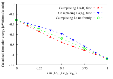
Figure 1: (Color online) Calculated formation energy of (La_1-xCe_x)₂Fe₁₄B via ab initio structure optimization utilizing OpenMX OpenMX .

Calculated formation energy for discretely substituted (La,Ce)₂Fe₁₄B is shown in Fig. 1 from ab initio structure optimization runs utilizing OpenMX OpenMX . The formation energy is based on the calculation of energy within the given standard pseudopotential data sets OpenMX . Calculated energy results for the reference elemental systems are given in Table 2 and those for the target stoichiometric compounds are in Table 3. Other discretely substituted materials, with Ce either replacing La($4f$) first or La($4g$) first, and substituting La($4f$) and La($4g$) on an equal footing (here we need two Ce atoms for one step of substitution and thus the step on the $x$ axis is $2~{}\mbox{(Ce atoms)}/8~{}\mbox{(host La sites)}=0.25$. The overall trend of Ce stabilizing the crystal structure is clearly seen and La($4f$) is energetically preferred by Ce.

material	$N_{\rm atom}$	$U_{\rm tot}~{}\mbox{[Hartree]}$
$\alpha$-B	36	$-105.056$
bcc-Fe	1	$-89.5730$
dhcp-La	4	$-161.9402$
fcc-Ce	1	$-53.9134$

Table 2: Calculated energy with OpenMX on the basis of the standard pseudopotentials OpenMX and the choice of basis sets as described in Sec. II for each elemental reference material. $N_{\rm atom}$ is the number of atoms in the unit cell. For all of the data in this table, the number of k points is $512$. Calculated energy for the reference elemental systems $\alpha$-B and bcc-Fe are taken from Ref. mm_20181228, .

material	$U_{\rm tot}~{}\mbox{[Hartree/(cell)]}$	$E_{\rm f}~{}\mbox{[eV/(f.u.)]}$
La2Fe14B	$-5351.689$	$-0.32$
Ce2Fe14B	$-5459.227$	$-1.08$

Table 3: Calculated energy with OpenMX on the basis of the standard pseudopotentials and the choice of basis sets as described in Sec. II.1.1 and the corresponding formation energy for each target material.

Before moving on to KKR-CPA results for the mixing energy, we compare the lattice as yielded from the structure optimization and the inputs to KKR-CPA as we empirically defined as is described in Sec. II.1.2. As the representative parameter to characterize the lattice, the data for the unit cell volume is shown in Fig. 2 together with the recent experimental results apl_2016 . We note that the materials with Ce preferentially substituting La($4f$) sites comes with a slightly smaller volume than the other cases of uniform substitution or Ce preferentially substituting La($4g$) sites. Such difference of unit cell volume depending on the site segregation has not been taken into account in the KKR-CPA calculations taking the interpolated lattice information based on past experimental data rmp_1991 as the input. Overestimate of the unit cell volume is seen in the optimized lattice while the overall trend with respect to Ce concentration goes in parallel between all of the optimized lattice, interpolated lattice in the input to KKR-CPA, and recent experimental measurement apl_2016 . Larger deviation seen at La₂Fe₁₄B between the recent experimental data, optimized lattice, and the past experiments rmp_1991 might be related to the less robust structure of La₂Fe₁₄B as seen in the relatively small absolute value of the calculated formation energy in Table 3 and Fig. 1.

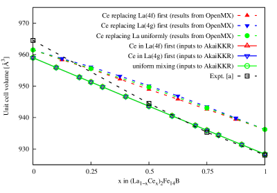
Figure 2: (Color online) Calculated unit-cell volume of (La_1-xCe_x)₂Fe₁₄B via ab initio structure optimization, the unit cell volume with the inputs to KKR-CPA on the interpolated lattices referring to experimental lattice in the literature rmp_1991 , and results from the latest experimental measurements apl_2016 as denoted by [a] in the figure.

Now we match the formation energy from the structure optimization and the other data from KKR-CPA. Those two data sets are presented in Fig. 3. We see that the results from the two approaches agree semi-quantitatively. Even with the small difference in the optimized cell volume depending on the site segregation of dopant Ce, we can presume that OpenMX data and AkaiKKR data are going in parallel concerning the energetics.

(a)

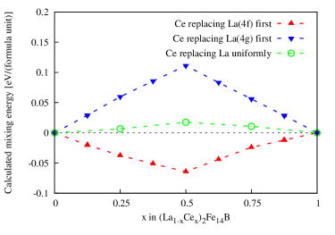
(b)

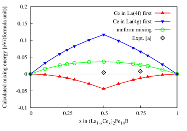
Figure 3: (Color online) Calculated mixing energy for (La_1-xCe_x)₂Fe₁₄B. (a) Results from the ab inito structure optimization utilizing OpenMX and (b) KKR-CPA utilizing AkaiKKR where results corresponding to the latest experimentally measured site segregation apl_2016 are denoted by [a] in the figure.

III.1.2 Magnetization

Calculated magnetization of (La_1-xCe_x)₂Fe₁₄B is shown in Fig. 4 as magnetic moments per formula unit. Taking into account the volume as shown in Fig. 2, the trend of magnetization in Tesla looks like Fig. 5. The latter should be used in the evaluation of the merit for permanent magnets.

(a)

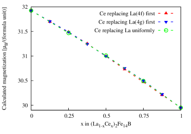
(b)

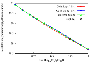
Figure 4: Calculated magnetization from (a) ab initio structure optimization and (b) KKR-CPA on the interpolated lattice between La₂Fe₁₄B and Ce₂Fe₁₄B. Results corresponding to the latest experimentally measured site segregation apl_2016 are denoted by [a] in the figure.

(a)

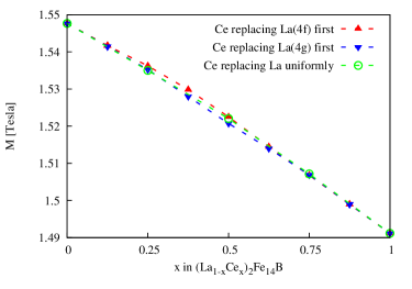
(b)

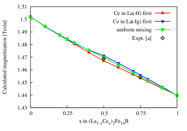
Figure 5: Calculated magnetization in Tesla from (a) ab initio structure optimization and (b) KKR-CPA on the interpolated lattice between La₂Fe₁₄B and Ce₂Fe₁₄B. Results corresponding to the latest experimentally measured site segregation apl_2016 are denoted by [a] in the figure.

In the results of structure optimization via OpenMX, we see that the small volume effect with Ce preferentially replacing La($4f$) sites as remarked in Sec. III.1.1 is reflected in the slight supremacy of magnetization in Tesla of the cases with Ce preferentially replacing La($4f$) sites over other case with Ce preferentially replacing La($4g$) sites. Remarkably, the energetically favorable substitution coincides with the case where a stronger magnetization in Tesla is reached due to the volume effect. This is a rare trend and is in contrast to typical situations where strong magnetization and structure stability is often traded off.

On the other hand KKR-CPA results via AkaiKKR do not incorporate the volume effect that can come from the doped site segregation, but the mixing ratio can be continuously swept on demand to see the overall trends including the experimental data points. While we systematically explored three representative case studies with uniform replacements and Ce preferentially replacing La($4f$) or La($4g$) sites, fractional ratio in the replacements was inspected in the recent experiments apl_2016 . Simulating such experimental mixing ratio within KKR-CPA, calculated magnetization is plotted in Fig. 4 (b) and 5 (b). It is seen that while energetically favorable replacements of La($4f$) by Ce dominates slightly shifted distribution over to the other energetically unfavorable La($4g$) site helps in lifting up the magnetization within the fixed lattice.

Since we do not exactly simulate the experimental observation at the moment it is not clear which physics of the above would be more dominating in real (La,Ce)₂Fe₁₄B. At least it is clear the particular site segregation is important in getting magnetization beyond a plainly interpolated magnetization between La₂Fe₁₄B and Ce₂Fe₁₄B.

III.1.3 Magnetic anisotropy energy

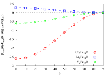
Figure 6: (Color online) Calculating magnetic anisotropy energy via fully relativistic calculation as implemented in OpenMX. Lines are fits to the calculated data points.

Results from fully relativistic calculations utilizing OpenMX with constraints on the direction of magnetization for stoichiometric compounds are shown in Fig 6. As a reference Y₂Fe₁₄B is included for which the structure optimization to extract the formation energy is presented in Ref. mm_20181228, . Optimized structure is taken from Sec. III.1.1 for La₂Fe₁₄B and Ce₂Fe₁₄B and the constraint on the direction of magnetization, as measured by an angle from the crystallographic $c$-axis of the R₂Fe₁₄B crystal rmp_1991 , is imposed to estimate the energy within the pseudopotential and the choice of the basis sets described in Sec. II.1.1.

In Fig. 6 calculated energy $\left.U_{\rm tot}[\mbox{R${}_{2}$Fe${}_{14}$B}]\right|_{\theta}$ is plotted with an offset taken at $\theta=90~{}\mbox{degrees}$. The fit to the calculated data obtained at every 10 degrees from $\theta=0$ to $\theta=90~{}\mbox{degrees}$ with the following relation

$$-K\left[(1-p-q)\cos^{2}\theta+p\cos^{4}\theta+q\cos^{6}\theta\right]$$ (1)

gives the anisotropy energy and the higher order contribution as tabulated in Table 4.

material	$K~{}\mbox{[meV/(f.u.)]}$	$p$	$q$
Ce2Fe14B	$2.609(7)$	$0.14(6)$	$-0.15(4)$
La2Fe14B	$-0.2819(1)$	$0.097(1)$	$q\equiv 0$
Y2Fe14B	$0.6034(2)$	$0.009(1)$	$q\equiv 0$

Table 4: Calculated magnetic anisotropy constants as defined in Eq. (1) in the text. The number in parenthesis is the error in the last digit from the data fit.

Numerically observed trends for uni-axial magnetic anisotropy are qualitatively consistent with the experimentally reported trends found in the literature expt_1985 where the strength of uni-axial magnetic anisotropy follows the order

$$\mbox{Ce${}_{2}$Fe${}_{14}$B}>\mbox{Y${}_{2}$Fe${}_{14}$B}>\mbox{La${}_{2}$Fe${}_{14}$B}.$$

We find easy-plane anisotropy in La₂Fe₁₄B which is by itself not entirely consistent with the experiments expt_1985 . Presumably in our calculations $3d$-electron anisotropy is underestimated and calculated anisotropy for La₂Fe₁₄B has not been strong enough but it is to be noted that actually La seems to contribute to the easy-plane anisotropy in La₂Fe₁₄B. It is also remarkable that higher-order terms up to the $3^{rd}$ order from delocalized $4f$-electrons in Ce₂Fe₁₄B and the $2^{nd}$ order terms in $d$-electron anisotropy can be quantitatively determined from first principles.

Uni-axial magnetic anisotropy energy contributed from itinerant $4f$-electrons in Ce₂Fe₁₄B are estimated to be in the order of 1 meV from 2 Ce atoms as seen in Fig. 6. This is not as large as the typical scale of MAE from RE like Nd, Sm, and Dy amounting to the order of 10 meV while an order of magnitude larger than the $3d$-electron anisotropy in the order of 0.1 meV per atom at maximum. Thus contribution to anisotropy coming from Ce in Ce-Fe intermetallics should definitely be exploited in fabricating an intermediate-grade magnet.

III.1.4 Curie temperature

Calculated Curie temperatures are shown in Fig 7 from KKR-CPA calculations.

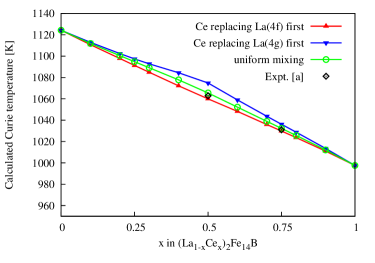
Figure 7: (Color online) Calculated Curie temperature for the interpolated-lattice compounds as addressed via KKR-CPA. Results corresponding to the latest experimentally measured site segregation apl_2016 are denoted by [a] in the figure.

At the stoichiometric limits, experimental Curie temperatures are rmp_1991 $T_{\rm Curie}[\mbox{La${}_{2}$Fe${}_{14}$B}]=530~{}\mbox{[K]}$ and 424 K for Ce₂Fe₁₄B. An overestimate for the absolute value of the Curie temperature by a factor close to $2$ is seen presumably due to the origins described in Sec. II.2.4 while the slope between La₂Fe₁₄B and Ce₂Fe₁₄B spanning $100~{}\mbox{[K]}$ is approximately reproduced.

III.2 Assessment of the merit of the light-rare-earth magnet

III.2.1 Referring to Nd₂Fe₁₄B

The intrinsic properties calculated above are compared to the counterpart data for Nd₂Fe₁₄B and the relative merit of (La_1-xCe_x)₂Fe₁₄B is assessed to inspect the optimal $x$.

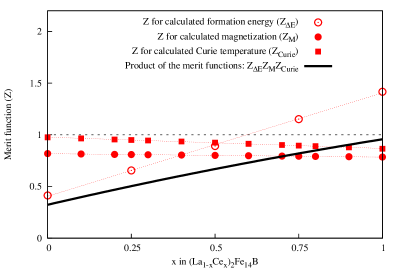
Figure 8: (Color online) Relative merit of (La_1-xCe_x)₂Fe₁₄B measured with respect to Nd₂Fe₁₄B for the formation energy, magnetization in Tesla, and Curie temperature based on our ab initio data.

We simply normalize the calculated formation energy, magnetization in Tesla, and Curie temperature of (La_1-xCe_x)₂Fe₁₄B by the counterpart data for Nd₂Fe₁₄B. Because the overall trend of the intrinsic properties as a function of $x$ more or less behaves overall in the same way irrespectively of the details of site segregation, we focus on the calculations with uniform replacements between La and Ce. For the formation energy, $\Delta E_{\rm f}[\mbox{Nd${}_{2}$Fe${}_{14}$B}]=-0.76~{}\mbox{[eV/(formula unit)]}$ is taken from Ref. mm_20181228, and define this ratio as the merit of formation energy which measures the merit in structure stability in terms of energetics. Also calculated magnetization in Tesla is compared to the counterpart results for Nd₂Fe₁₄B mm_2018 ; mm_20181228 . For Nd₂Fe₁₄B in the ground state $M_{s}=1.836~{}\mbox{[Tesla]}$ to which our ab initio calculated magnetization in the ground state is referred. Concerning the Curie temperature of Nd₂Fe₁₄B, the same set-up of KKR-CPA as is done for (La,Ce)₂Fe₁₄B gives $T_{\rm Curie}=1152.743~{}\mbox{[K]}$, which should be carefully compared with the experimental data $T_{\rm Curie}=585~{}\mbox{[K]}$ rmp_1991 . Thus defined merit of (La_1-xCe_x)₂Fe₁₄B concerning formation energy, magnetization, and Curie temperature is shown in Fig. 8. It is seen that the merit is gained mostly due to the formation energy and monotonically increasing with respect to $x$ based on the plain definition of the merit function only referring to Nd₂Fe₁₄B within ab initio data.

Since all of the intrinsic properties are prerequisites, we have taken a product of the merit function for each of formation energy, magnetization, and Curie temperature rather than taking a sum. It is not very straightforward to define the merit of magnetic anisotropy energy on our ab initio data because we have the data only for the stoichiometric limits. On top of that, a data set for anisotropy energy calculated for Nd₂Fe₁₄B would be based on the effects of crystal fields acting on very well localized $4f$ electrons. The mechanism of magnetic anisotropy is different between (La,Ce)₂Fe₁₄B and Nd₂Fe₁₄B. It is not quite straightforward to take a data set for magnetic anisotropy on an equal footing for the materials with delocalized $4f$-electrons and for the other bunch of materials with very well localized $4f$-electrons. We will not take a very close look at anisotropy here due to this fundamental problem and practically due to the trend seen in Fig. 8 which is monotonically-increasing with respect to $x$. Here further inclusion of magnetic anisotropy energy would not qualitatively alter the message of the merit. Rather the range of the practical operation temperature seems to put the most stringent constraint on the merit function and make it non-monotonic as we see below in Sec. III.2.2.

III.2.2 Considering the operation temperature range

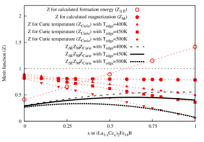
Figure 9: (Color online) Relative merit of (La_1-xCe_x)₂Fe₁₄B measured with respect to Nd₂Fe₁₄B. The overall merit involving formation energy, magnetization, and Curie temperature is quantitatively controlled by the position of the upper temperature limit $T_{\rm edge}$ of practical usage. Merit for three cases, $T_{\rm edge}=400~{}\mbox{K}$, $450~{}\mbox{[K]}$, and $500~{}\mbox{[K]}$ are presented.

Permanent magnets are basically put into practical use around room temperatures and the critical interest lies in the magnetic properties at the high-temperature edge of the temperature range: $300~{}\mbox{[K]}\leq T\leq T_{\rm edge}~{}\mbox{[K]}$. For traction motors in vehicles $T_{\rm edge}\simeq 450~{}\mbox{[K]}$. A ferromagnet with the Curie temperature below $T_{\rm edge}$ would not be acceptable in practice. Thus we define the merit function concerning the Curie temperature, which we will denote by $Z_{\rm curie}$ below, in such a way that the merit becomes unity at the Curie temperature of Nd₂Fe₁₄B and zero at $T_{\rm Curie}(x)=T_{\rm edge}$. A way to define this would be the following:

$$Z_{\rm Curie}(x) \equiv \frac{T^{\rm adjusted}_{\rm Curie}(x)}{T^{\rm expt.}_{\rm Curie}[\mbox{Nd${}_{2}$Fe${}_{14}$B}]}$$ (2)

$$\times\frac{T_{\rm Curie}^{\rm adjusted}(x)-T_{\rm edge}}{T_{\rm Curie}[\mbox{Nd${}_{2}$Fe${}_{14}$B}]-T_{\rm edge}}$$

$$T^{\rm adjusted}_{\rm Curie}(x) \simeq T^{\rm calc}_{\rm Curie}(x)\frac{T^{\rm expt.}_{\rm Curie}[\mbox{Nd${}_{2}$Fe${}_{14}$B}]}{T^{\rm calc.}_{\rm Curie}[\mbox{Nd${}_{2}$Fe${}_{14}$B}]}$$ (3)

It is plotted in Fig. 9 incorporating the experimental data $T^{\rm expt.}_{\rm Curie}[{\rm Nd_{2}Fe_{14}B}]=585~{}\mbox{[K]}$ rmp_1991 and picking up several choices for $T_{\rm edge}$ between $400~{}\mbox{[K]}$ and $500~{}\mbox{[K]}$. The higher (lower) the operation temperature range spans, less (more) amount of Ce gives a more reasonable choice, respectively. We see that when the high temperature edge is set at 450 K, the merit function shows a broad maximum around 70% of Ce. This particular optimal chemical composition may be compared with the messages from the recent developments for Ce-based core-shell magnet ito_2016 which points to an optimal amount of Ce to be 75% as investigated with the room temperature performance shoji_2018 .

The above arguments depend on how we define the merit function up to the location of the high temperature edge. The merit function can be further generalized via possible data assimilation to incorporate extrinsic parameters, even the cost of the fabrication. In the present study we have restricted ourselves to an evaluation of the intrinsic properties of magnetism.

IV Discussions

IV.1 Utility of Ce

Obvious merit brought about by Ce has been in the structure stabilization and the biggest drawback was coming from Curie temperature. During the course of our calculations we notice the tiny enhancement of magnetization as measured in Tesla in the results of ab initio structure optimization as shown in Fig. 5 (a). Even though the magnetization as measured in terms of magnetic moments per atoms may be on a par as seen in Fig. 4 (a), the particular volume shrinkage can help in enhancing the merit of the material. Even if $4f$-electrons may not contribute to the intrinsic magnetism explicitly these indirect help as a useful spacer should not be overlooked.

IV.2 Valence state of Ce

In the present work we have assumed that Ce stays in the tetravalent state. On the other hand, trends toward trivalent state of Ce in an expanded space may well be suspected, especially when Ce replaces the slightly larger La($4g$) site. Generally speaking, it seems unlikely for the $4f$ electron state of Ce to be able to remain localized if the conduction band is widely exchange split. The location of localized $4f$-level in Ce is around 2 eV below the Fermi level while the exchange splitting can span a range of few electron volts. Thus it is naively expected that in Ce-Fe intermetallic ferromagnets $f$-$d$ hybridization would be too strong to allow for localized $4f$-electrons in Ce unless some fine tuning of particular electronic clouds is implemented for some mechanism possibly exploiting magnetic anisotropy. At the moment we are not aware of such cases but do not entirely rule out the possibility for trivalent state in Ce-Fe (or Ce-Co) intermetallics. Separate calculations assisted by a dynamical mean field theory to describe the correlated electron nature in Ce for a fictitious Ce₂Cu₁₄B on the La₂Fe₁₄B lattice mm , which is constructed so that the localization of $4f$ electron in Ce would get more likely with the largest lattice constant and vanishing splitting of the conduction electrons, have showed no sign of trivalent Ce. Presumably the lattice structure of R₂Fe₁₄B may not be optimal for the localization of $4f$-electrons in Ce.

V Conclusions and outlook

We have figured out the merit of light-rare-earth permanent magnet (La,Ce)₂Fe₁₄B from first principles by incorporating the prerequisite condition for practical utility referring to the experimental Curie temperature. With the commonplace high temperature edge at 450 K in practical applications of rare earth permanent magnets, the best compromise has been found at the concentration of Ce around 70%.

We have purged Co out of the present scope to clarify the $4f$-electron physics in the valence state combined with $3d$-electron ferromagnetism - this has been to assess the maximum possible merit of ferromagneism from first principles with abundant elements. Inclusion of Co does help at least in raising the Curie temperature rmp_1991 as long as the extra cost for Co would not be too big a problem. Exploration of the extended chemical composition space for R₂(Fe,Co)₁₄B (R=rare earth including La and Ce) in quest of peak performance in uni-axial ferromagnetism will be reported in a separate work harashima .

- (1) M. Sagawa, S. Fujimura, N. Togawa, H. Yamamoto, and Y. Matsuura, J. Appl. Phys. 55, 2083 (1984).
- (2) J. J. Croat, J. F. Herbst, R. W. Lee, and F. E. Pinkerton, J. Appl. Phys. 55, 2078 (1984).
- (3) For a review, see J. F. Herbst, Rev. Mod. Phys. 63, 819 (1991).
- (4) C. V. Colin, M. Ito, M. Yano, N. M. Dempsey, E. Suard, and D. Givord, Appl. Phys. Lett. 108, 242415 (2016).
- (5) See H. C. Ku, G. P. Meisner, F. Acker, D. C. Johnston, Solid State Communications 35, 91 (1980) for the discovery of the material, S. K. Dhar, S. K. Malik, R. Vijayaraghavan, J. Phys. C: Solid State Phys. 14 L321 (1981) for the observation of the exceptionally high Curie temperature, H. N. Kono and Y. Kuramoto, J. Phys. Soc. Jpn. 75, 084706 (2006); H. N. Kono, Ph. D thesis (Tohoku Univ., 2006); K. Yamauchi, A. Yanase, H. Harima, J. Phys. Soc. Jpn. 79, 044717 (2010) for one of the most up-to-date picture of the electronic structure involving -electrons.
- (6) http://www.openmx-square.org
- (7) T. Ozaki, Phys. Rev. B. 67, 155108, (2003).
- (8) T. Ozaki and H. Kino, Phys. Rev. B 69, 195113 (2004).
- (9) T. Ozaki and H. Kino, Phys. Rev. B 72, 045121 (2005).
- (10) T. V. T. Duy and T. Ozaki, Comput. Phys. Commun. 185, 777 (2014).
- (11) K. Lejaeghere, G. Bihlmayer, T. Björkman, P. Blaha, S. Blügel, V. Blum, D. Caliste, I.E. Castelli, S.J. Clark, A. Dal Corso, S. de Gironcoli, T. Deutsch, J.K. Dewhurst, I. Di Marco, C. Draxl, M. Dułak, O. Eriksson, J.A. Flores-Livas, K.F. Garrity, L. Genovese, P. Giannozzi, M. Giantomassi, S. Goedecker, X. Gonze, O. Grånäs, E.K. Gross, A. Gulans, F. Gygi, D.R. Hamann, P.J. Hasnip, N.A. Holzwarth, D. Iu̧san, D.B. Jochym, F. Jollet, D. Jones, G. Kresse, K. Koepernik, E. Küçükbenli, Y.O. Kvashnin, I.L. Locht, S. Lubeck, M. Marsman, N. Marzari, U. Nitzsche, L. Nordström, T. Ozaki, L. Paulatto, C.J. Pickard, W. Poelmans, M.I. Probert, K. Refson, M. Richter, G.M. Rignanese, S. Saha, M. Scheffler, M. Schlipf, K. Schwarz, S. Sharma, F. Tavazza, P. Thunström, A. Tkatchenko, M. Torrent, D. Vanderbilt, M.J. van Setten, V. Van Speybroeck, J.M. Wills, J.R. Yates, G.X. Zhang, and S. Cottenier, Science 351, aad3000 (2016).
- (12) I. Morrison, D.M. Bylander, L. Kleinman, Phys. Rev. B 47, 6728 (1993).
- (13) G. Theurich and N.A. Hill, Phys. Rev. B 64, 073106 (2001).
- (14) J. Korringa, Physica 13, 392 (1947).
- (15) W. Kohn and N. Rostoker, Phys. Rev. 94, 1111 (1954).
- (16) H. Shiba, Prog. Theor. Phys. 46, 77 (1971); H. Akai, Physica 86 – 88B, 539 (1977).
- (17) http://kkr.issp.u-tokyo.ac.jp/
- (18) P. Hohenberg and W. Kohn, Phys. Rev. 136, B864 (1964).
- (19) W. Kohn and L. Sham, Phys. Rev. 140, A1133 (1965)
- (20) J. P. Perdew, K. Burke, and M. Ernzerhof, Phys. Rev. Lett. 77, 3865 (1996).
- (21) V. L. Moruzzi, J. F. Janak, and A. R. Williams, Calculated Properties of Metals (Pergamon Press, New York, 1978).
- (22) K. Saito, S. Doi, T. Abe, K. Ono, J. Alloys Compds. 721, 476 (2017).
- (23) R. Zeller, J. Phys. Condens. Matter 25, 105505 (2013).
- (24) M. Ogura, A. Mashiyama, H. Akai, J. Phys. Soc. Jpn. 84, 084702 (2015).
- (25) A. I. Liechtenstein, M. I. Katsnelson, V. P. Antropov, and V. A. Gubanov, J. Mag. Mag. Mater. 67, 65 (1987).
- (26) M. Matsumoto and H. Akai, preprint [arXiv:1812.04842].
- (27) A. Terasawa et al., in preparation.
- (28) Y. Harashima et al., in preparation.
- (29) M. Matsumoto, preprint [arXiv:1812.10945].
- (30) R. Grössinger, X. Sun, R. Eibler, K. Buschow, H. Kirchmayr, Journal de Physique Colloques, 46 (C6), C6-221 (1985).
- (31) M. Ito, M. Yano, N. Sakuma, H. Kishimoto, A. Manabe, T. Shoji, A. Kato, N. M. Dempsey, D. Givord, and G. T. Zimanyi, AIP Advances 6, 056029 (2016).
- (32) T. Shoji et al., Journal of Society of Automotive Engineers of Japan, 72, 102 (2018) (in Japanese); https://newsroom.toyota.co.jp/en/corporate/21139684.html
- (33) MM, in preparation.