A convergent numerical method for a multi-frequency inverse source problem in inhomogenous media

Abstract

A new numerical method to solve an inverse source problem for the Helmholtz equation in inhomogenous media is proposed. This method reduces the original inverse problem to a boundary value problem for a coupled system of elliptic PDEs, in which the unknown source function is not involved. The Dirichlet boundary condition is given on the entire boundary of the domain of interest and the Neumann boundary condition is given on a part of this boundary. To solve this problem, the quasi-reversibility method is applied. Uniqueness and existence of the minimizer are proven. A new Carleman estimate is established. Next, the convergence of those minimizers to the exact solution is proven using that Carleman estimate. Results of numerical tests are presented.

Key words: Inverse source problem, truncated Fourier series, approximation, Carleman estimate, convergence.

AMS subject classification: 35R30, 78A46.

1 Introduction and the problem statement

In this paper, we propose a new numerical method to solve an inverse source problem for the Helmholtz equation in the multi-frequency regime. This is the problem of determining the unknown source from external measurement of the wave field. It is worth mentioning that the inverse source problem has uncountable real-world applications in electroencephalography, biomedical imaging, etc., see e.g., [1, 2, 3, 14, 18, 21, 19].

Below $\mathbf{x}=\left(x_{1},...,x_{n-1},z\right)\in\mathbb{R}^{n}.$ Let $\Omega$ be the cube $(-R,R)^{n}\subset\mathbb{R}^{n}$, $R\geq 1$, and

$$\Gamma_{+}=\{\mathbf{x}\in\partial\Omega:z=R\}.$$ (1.1)

For $i,j=1,...,n$, let functions $a_{ij}\in C^{1}(\mathbb{R}^{n}),b_{j}\in C(\mathbb{R}^{n}),c\in C(\mathbb{R}^{n})$ be such that:

1. For all $\mathbf{x}\in\mathbb{R}^{n}$

   $$a_{ij}(\mathbf{x})=a_{ji}(\mathbf{x})\quad 1\leq i,j\leq n.$$ (1.2)

2. There exist two constants $\mu_{1}$ and $\mu_{2}$ such that $0<\mu_{1}\leq\mu_{2}$ and

   $$\mu_{1}|\mathbf{\xi}|^{2}\leq\sum_{i,j=1}^{n}a_{ij}\left(\mathbf{x}\right)\xi_{i}\xi_{j}\leq\mu_{2}|\mathbf{\xi}|^{2}\quad\mbox{for all }\mathbf{x}\in\mathbb{R}^{n},\mathbf{\xi}\in\mathbb{R}^{n}.$$ (1.3)

3. For all $\mathbf{x}\in\mathbb{R}^{n}\setminus\Omega$

   $$a_{ij}(\mathbf{x})=\left\{\begin{array}[]{ll}1&\mbox{if }i=j,\\ 0&\mbox{if }i\neq j.\end{array}\right.$$ (1.4)

4. For all $\mathbf{x}\in\mathbb{R}^{n}\setminus\Omega$,

   $$b_{j}(\mathbf{x})=c(\mathbf{x})=0.$$ (1.5)

We introduce the uniformly elliptic operator $L$ as follows

$$Lu=\sum_{i,j=1}^{n}a_{ij}(\mathbf{x})u_{x_{i}x_{j}}+\sum_{i=1}^{n}b_{i}(\mathbf{x})u_{x_{i}}+c(\mathbf{x})u\quad\mbox{for }u\in H^{2}(\mathbb{R}^{n}).$$ (1.6)

The principal part of this operator is

$$L_{0}u=\sum_{i,j=1}^{n}a_{ij}(\mathbf{x})u_{x_{i}x_{j}}.$$ (1.7)

Let $k>0$ be the wave number and $u=u(\mathbf{x},k)$ be the complex valued wave field of wave number $k$, generated by the source function which has the form of separable variables $g(k)f(\mathbf{x}),$ where functions $g\in C^{1}[0,\infty)$ and $f\in C^{1}\left(\mathbb{R}^{n}\right)$. The wave field $u(\mathbf{x},k)\in C^{2}(\mathbb{R}^{n}),k>0,$ satisfies the equation

$$Lu+k^{2}\mathbf{n}^{2}(\mathbf{x})u(\mathbf{x},k)=g(k)f(\mathbf{x}),\quad\mathbf{x}\in\mathbb{R}^{n}$$ (1.8)

and the Sommerfeld radiation condition

$$\partial_{|\mathbf{x}|}u(\mathbf{x},k)-\mathrm{i}ku(\mathbf{x},k)=o(|\mathbf{x}|^{(1-n)/2}),\quad|\mathbf{x}|\rightarrow\infty.$$ (1.9)

Here, the function $\mathbf{n}\in C^{1}(\mathbb{R}^{n})$ is the refractive index . We assume that

$$\mathbf{n}\left(\mathbf{x}\right)=1\quad\quad\mbox{for }\mathbf{x}\in\mathbb{R}^{n}\setminus\Omega.$$ (1.10)

See [16] for the well-posedness of problem (1.8)–(1.9) in the case $L=\Delta$. Given numbers $\underline{k}$ and $\overline{k}$ such that $0<\underline{k}<\overline{k}<\infty$ and assuming that the function $g:[\underline{k},\overline{k}]\rightarrow\mathbb{R}$ is known, we are interested in the following problem.

Problem 1.1 (Inverse source problem with Cauchy data).

Assume that conditions (1.1)-(1.10) are in place. Reconstruct the function $f(\mathbf{x})$ for $\mathbf{x}\in\Omega$, given the functions $F$ and $G$, where

$$F(\mathbf{x},k) =u(\mathbf{x},k),\quad\mathbf{x}\in\partial\Omega,k\in(\underline{k},\overline{k}),$$ (1.11)

$$G(\mathbf{x},k) =\partial_{z}u(\mathbf{x},k),\quad\mathbf{x}\in\Gamma_{+},k\in(\underline{k},\overline{k}),$$ (1.12)

where $u(\mathbf{x},k)$ is the solution of problem (1.8), (1.9).

Problem 1.1 is somewhat over-determined due to the additional data $G(\mathbf{x},k)$ measured on $\Gamma_{+}\times[\underline{k},\overline{k}]$. We need this data for the convergence theorem. However, we notice in our numerical experiments that our method works well without that additional data. More precisely, in addition to Problem 1.1, we also consider the following non-overdetermined problem.

Problem 1.2 (Inverse source problem with Dirichlet data).

Assume that conditions (1.1)-(1.10) are in place. Reconstruct the functions $f(\mathbf{x})$, $\mathbf{x}\in\Omega$, given the following data

$$F(\mathbf{x},k)=u(\mathbf{x},k),\quad\mathbf{x}\in\partial\Omega,k\in(\underline{k},\overline{k}),$$ (1.13)

where $u(\mathbf{x},k)$ is the solution of (1.8)–(1.9).

Remark 1.1.

In fact, the Dirichlet boundary data (1.13) implicitly contain the Neumann boundary data for the function $u$ on the entire boundary $\partial\Omega.$ Indeed, for each $k\in(\underline{k},\overline{k})$ one can uniquely solve equation (1.8) with the radiation condition (1.9) and boundary condition (1.13) in the unbounded domain $\mathbb{R}^{n}\setminus\Omega.$ The resulting solution provides the Neumann boundary condition $\partial_{\nu}u(\mathbf{x},k)$ for $\mathbf{x}\in\partial\Omega,$ $k\in(\underline{k},\overline{k}),$ where $\nu$ is the unit outward normal vector at $\partial\Omega.$

This and similar inverse source problems for Helmholtz-like PDEs were studied both analytically and numerically in [3, 22]. In particular, in works [20, 22] uniqueness and stability results were proven for the case of constant coefficients in (1.8) and it was also shown that the stability estimate improves when the frequency grows. In [23] uniqueness was proven for non constant coefficients. To the best of our knowledge, past numerical methods for these problems are based on various methods of the minimization of mismatched least squares functionals. Good quality numerical solutions are obtained in [4, 5, 23]. However, those minimization procedures do not allow to establish convergence rates of minimizers to the exact solution when the noise in the data tends to zero. On the other hand, we refer here to the work [42, 44, 45, 47, 48], in which a non-iterative method, based on a fresh idea, was proposed to solve the inverse source problem for a homogenous medium. This method is called the Fourier method for solving multifrequency inverse source problems. Uniqueness and stability results were proven in [44] and good quality numerical results were presented. We would like to refer the reader to [13, 38, 39, 43, 46] for some works studying inverse source problems that are related to the inverse problems in this paper.

In this paper, we solve the inverse source problem for inhomogeneous media. We propose a new numerical method which enables us to establish convergence rate of minimizers of a certain functional of the Quasi-Reversibility Method (QRM) to the exact solution, as long as the noise in the data tends to zero. Our method is based on four ingredients:

1. Elimination of the unknown source function $f\left(\mathbf{x}\right)$ from the original PDE via the differentiation with respect to $k$ of the function $u(\mathbf{x},k)/g\left(k\right).$

2. The use of a newly published [30] orthonormal basis in $L^{2}\left(\underline{k},\overline{k}\right)$ to obtain an overdetermined boundary value problem for a system of coupled elliptic PDEs of the second order.

3. The use of the QRM to find an approximate solution of that boundary value problem.

4. The formulation and the proof of a new Carleman estimate for the operator $L_{0}$ in (1.7).

5. In the case of Problem 1.1, the use of this Carleman estimate for establishing the convergence rate of the minimizers of the QRM to the exact solution, as long as the noise in the data tends to zero.

Recently a similar idea was applied to develop a new numerical method for the X-ray computed tomography with a special case of incomplete data [33] as well as to the development of a globally convergent numerical method for a 1D coefficient inverse problem [31]. The above items 1, 4 and 5 have roots in the Bukhgeim-Klibanov method, which was originally introduced in [12]. Even though there exists now a significant number of publications on this method, we refer here only to a few of them [7, 8, 35, 28] since the current paper is not about that method. The original goal of [12] was to prove uniqueness theorems for coefficient inverse problems. Nowadays, however, ideas of this method are applied for constructions of numerical methods for coefficient inverse problems and other ill-posed problems, see, e.g. [30, 31, 32, 36].

The quasi-reversibility method was first introduced by Latts and Lions in [37] for numerical solutions of ill-posed problems for partial differential equations. It has been studied intensively since then, see e.g., [6, 9, 10, 11, 15, 17, 27, 34, 28, 40]. A survey on this method can be found in [29]. The solution of the system of the above item 2 due to the quasi-reversibility method is called regularized solution in the theory of ill-posed problems [41]. Thus, by item 5 a new Carleman estimate allows us to prove convergence of regularized solutions to the exact one as the noise in the data tends to zero. We do this only for 1.1. In contrast we do not investigate convergence of our method for Problem 1.2. This problem is studied only numerically below.

The paper is organized as follows. In Section 2, we present the numerical methods to solve Problems 1.1 and 1.2. Next, in Section 3, we discuss about the QRM for Problem 1.1. We prove a new Carleman estimate in Section 4. In section 5, we prove the convergence of the regularized solutions to the true one. In Section 6, we describe the numerical implementations for both Problems 1.1 and 1.2 and present numerical results.

2 Numerical Methods for Problems 1.1 and 1.2

We first recall a special basis of $L^{2}(\underline{k},\overline{k}),$ which was first introduced in [30].

2.1 A special orthonormal basis in $L^{2}(\underline{k},\overline{k})$

For each $m\geq 1$, define $\phi_{m}(k)=(k-k_{0})^{m-1}\exp(k-k_{0})$ where $k_{0}=(\underline{k}+\overline{k})/2$. The sequence $\{\phi_{m}\}_{m=1}^{\infty}$ is complete in $L^{2}(\underline{k},\overline{k})$. Applying the Gram-Schmidt orthonormalization procedure to the sequence $\{\phi_{m}\}_{m=1}^{\infty}$, we obtain an orthonormal basis in $L^{2}(\underline{k},\overline{k}),$ denoted by $\{\Psi_{m}\}_{m=1}^{\infty}$. It is not hard to verify that for each $m,$ the function $\Psi_{m}(k)$ has the form

$$\Psi_{m}(k)=P_{m-1}(k-k_{0})\exp(k-k_{0}),$$

where $P_{m-1}$ is a polynomial of the degree $(m-1)$. This leads to the following result, which plays an important role in our analysis.

Proposition 2.1 (see [30]).

For $m,r\geq 1$, we have

$$d_{mr}=\int_{\underline{k}}^{\overline{k}}\Psi_{m}(k)\Psi_{r}^{\prime}(k)dk=\left\{\begin{array}[]{ll}1&\mbox{if }r=m,\\ 0&\mbox{if }r<m.\end{array}\right.$$ (2.1)

Consequently, let $N>1$ be an integer. Then the $N\times N$ matrix

$$D_{N}=(d_{mr})_{m,r=1}^{N}$$ (2.2)

has determinant $1$ and is invertible.

Remark 2.1.

The basis $\{\Psi_{m}\}_{m=1}^{\infty}$ was first introduced in [30]. Then, it was successfully used to numerically solve nonlinear coefficient inverse problems [32, 31] and the inverse problem of X-ray tomography with incomplete data [33].

2.2 Truncated Fourier series

Assume that in (1.8) $g(k)\neq 0,\forall k\in[\underline{k},\overline{k}]$. Introduce the function $v(\mathbf{x},k),$

$$v(\mathbf{x},k)=\frac{u(\mathbf{x},k)}{g(k)},\quad\mathbf{x}\in\Omega,k\in[\underline{k},\overline{k}].$$ (2.3)

Let $L$ be the elliptic operator defined in (1.6). By (1.8)

$$L\left(v(\mathbf{x},k)\right)+k^{2}\mathbf{n}^{2}\left(\mathbf{x}\right)v(\mathbf{x},k)=f(\mathbf{x}),\quad\mathbf{x}\in\Omega,k\in[\underline{k},\overline{k}].$$ (2.4)

To eliminate the unknown right hand side $f(\mathbf{x})$ from equation (2.4), we differentiate it with respect to $k$ and obtain

$$L\left(\partial_{k}v(\mathbf{x},k)\right)+k^{2}\mathbf{n}^{2}(\mathbf{x})\partial_{k}v(\mathbf{x},k)+2k\mathbf{n}^{2}(\mathbf{x})v(\mathbf{x},k)=0,\quad\mathbf{x}\in\Omega,k\in[\underline{k},\overline{k}].$$ (2.5)

It follows from (1.11), (1.12) and (2.3) that in the case of Problem 1.1 the function $v$ satisfies the following boundary conditions

$$v(\mathbf{x},k)=\frac{F(\mathbf{x},k)}{g(k)},\text{ \ \ }\mathbf{x}\in\partial\Omega,k\in[\underline{k},\overline{k}],$$ (2.6)

$$\partial_{z}v(\mathbf{x},k)=\frac{G(\mathbf{x},k)}{g(k)},\quad\mathbf{x}\in\Gamma_{+},k\in[\underline{k},\overline{k}].$$ (2.7)

In Problem 1.2 only condition (2.6) holds.

Fix an integer $N\geq 1$. Recalling the orthonormal basis $\{\Psi_{r}\}_{r=1}^{\infty}$ of $L^{2}(\underline{k},\overline{k})$ in Section 2.1, we approximate

$$v(\mathbf{x},k) =\sum_{m=1}^{N}v_{m}(\mathbf{x})\Psi_{m}(k)\quad\mathbf{x}\in\Omega,k\in[\underline{k},\overline{k}],$$ (2.8)

$$\partial_{k}v(\mathbf{x},k) =\sum_{m=1}^{N}v_{m}(\mathbf{x})\Psi_{m}^{\prime}(k)\quad\mathbf{x}\in\Omega,k\in[\underline{k},\overline{k}],$$ (2.9)

where

$$v_{m}(\mathbf{x})=\int_{\underline{k}}^{\overline{k}}v(\mathbf{x},k)\Psi_{m}(k)dk\quad\mathbf{x}\in\Omega,m=1,2,\dots,N.$$ (2.10)

Remark 2.2.

Similarly with [30, 32, 31, 33], we assume here that the truncated Fourier series (2.8) satisfies equation (2.4) and that truncated Fourier series (2.8) and (2.9), taken together, satisfy equation (2.5). This is our approximate mathematical model. Since we work with a numerical method, we accept this approximation scheme. Our main goal below is to find numerically Fourier coefficients $v_{m}(\mathbf{x}),$ $m=1,2,\dots,N,$ of $v(\mathbf{x},k)$, see (2.10). If those Fourier coefficients are approximated, the target unknown function $f(\mathbf{x})$ can be approximated as the right hand side of (2.4).

Remark 2.3.

The number $N$ is chosen numerically. Proving convergence of our method as $N\rightarrow\infty$ is very challenging and such proofs are very rare in the field of ill-posed problems. Indeed, the intrinsic reason of this is the ill-posedness of those problems. Therefore, we omit the proof of convergence of our method as $N\rightarrow\infty.$ Nevertheless, a rich numerical experience of a number of previous publications, see, e.g. [25, 26, 24, 36, 32, 31, 33] indicates that this truncation technique still leads to good numerical results.

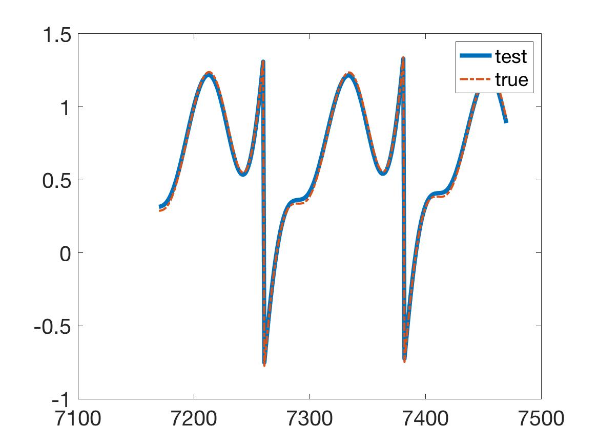
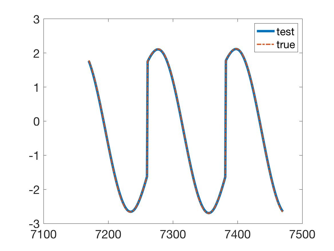
We now compare numerically the true function $v(\mathbf{x},k)$ with its approximation (2.8). and observe that their difference is small, see Figure 1 for the illustration.

(a) The real parts of the true and test functions

(b) The imaginary parts of the true and test functions

Figure 1: The comparison of the true function $v(\cdot,k=1.5)=\sum_{m=1}^{\infty}v_{m}(\mathbf{x})\Psi_{m}(k)$ and the test function $\sum_{m=1}^{10}v_{m}(\cdot)\Psi_{m}(k)$ in Test 5, see Section 4. In this test, we consider the case $n=2$ and $\Omega=(-2,2)^{2}$. On $\Omega,$ we arrange a uniform grid of $121\times 121$ points in $\Omega$. Those points are numbered from $1$ to $121^{2}$. In (a) and (b), we respectively show the real and imaginary parts of the two functions at 300 points numbered from 7170 to 7470. It is evident that reconstructing the first 10 terms of the Fourier coefficients of $v(\mathbf{x},k)$ is sufficient to solve our inverse source problems.

Plugging (2.8) and (2.9) in equation (2.5), we obtain

$$\sum_{r=1}^{N}\left(Lv_{r}\left(\mathbf{x}\right)\right)\Psi_{r}^{\prime}(k)+\sum_{r=1}^{N}\left(\mathbf{n}^{2}(\mathbf{x})v_{r}\left(\mathbf{x}\right)\right)\left(k^{2}\Psi_{r}^{\prime}(k)+2k\Psi_{r}(k)\right)=0,\text{ }\mathbf{x}\in\Omega.$$ (2.11)

For each $m=1,...,N$, we multiply both sides of (2.11) by the function $\Psi_{m}(k)$ and then integrate the resulting equation with respect to $k\in\left(\underline{k},\overline{k}\right).$ We obtain

$$\sum_{r=1}^{N}\left(Lv_{r}\left(\mathbf{x}\right)\right)\int_{\underline{k}}^{\overline{k}}\Psi_{r}^{\prime}(k)\Psi_{m}(k)dk$$

$$+\sum_{r=1}^{N}\left(\mathbf{n}^{2}(\mathbf{x})v_{r}\left(\mathbf{x}\right)\right)\int_{\underline{k}}^{\overline{k}}\left(k^{2}\Psi_{r}^{\prime}(k)+2k\Psi_{r}(k)\right)\Psi_{m}(k)dk=0$$ (2.12)

for all $\mathbf{x}\in\Omega$, $m=1,2,\dots,N.$ Denote

$$V(\mathbf{x})=(v_{1}(\mathbf{x}),v_{2}(\mathbf{x}),\cdots,v_{N}(\mathbf{x}))^{T}\quad\mathbf{x}\in\Omega,$$ (2.13)

$$S_{N}=\left(s_{mr}\right)_{m,r=1}^{N},\quad\mbox{with }s_{mr}=\int_{\underline{k}}^{\overline{k}}\left(k^{2}\Psi_{r}^{\prime}(k)+2k\Psi_{r}(k)\right)\Psi_{m}(k)dk.$$ (2.14)

Then, (2.2), (2.12)-(2.14) imply

$$D_{N}L\left(V\left(\mathbf{x}\right)\right)+S_{N}\mathbf{n}^{2}(\mathbf{x})V(\mathbf{x})=0,\text{ \ }\mathbf{x}\in\Omega,$$ (2.15)

Denote

$$\widetilde{F}(\mathbf{x}) =\left(\int_{\underline{k}}^{\overline{k}}\frac{F(\mathbf{x},k)}{g(k)}\Psi_{1}(k)dk,\dots,\int_{\underline{k}}^{\overline{k}}\frac{F(\mathbf{x},k)}{g(k)}\Psi_{N}(k)dk\right)^{T},\quad\mathbf{x}\in\partial\Omega,$$ (2.16)

$$\widetilde{G}(\mathbf{x}) =\left(\int_{\underline{k}}^{\overline{k}}\frac{G(\mathbf{x},k)}{g(k)}\Psi_{1}(k)dk,\dots,\int_{\underline{k}}^{\overline{k}}\frac{G(\mathbf{x},k)}{g(k)}\Psi_{N}(k)dk\right)^{T},\quad\mathbf{x}\in\Gamma_{+}.$$ (2.17)

It follows from (2.6) and (2.7) that in the case of 1.1 the vector function $V(\mathbf{x})$ satisfies the following two boundary conditions:

$$V\left(\mathbf{x}\right)=\widetilde{F}(\mathbf{x}),\text{ }\mathbf{x}\in\partial\Omega,$$ (2.18)

$$\partial_{\nu}V\left(\mathbf{x}\right)=\widetilde{G}(\mathbf{x}),\text{ }\mathbf{x}\in\Gamma_{+}.$$ (2.19)

And in the case of 1.2 only boundary condition (2.18) takes place.

These arguments lead to Algorithms 1 and 2 to solve Problems 1.1 and 1.2 respectively.

Algorithm 1 The procedure to solve Problem 1.1

1:  Choose a number $N$. Construct the functions $\Psi_{m}$, $1\leq m\leq N,$ in Section 2.1 and compute the matrix $D_{N}$ as in Proposition 2.1.

2:  Calculate the boundary data $\widetilde{F}$ and $\widetilde{G}$ for the vector valued function $V$ via (2.16) and (2.17) respectively.

3:  Find an approximate solution of the system (2.15), (2.18) and (2.19) via the quasi-reversibility method.

4:  Having $V=(v_{1},v_{2},\dots,v_{N})^{T}$ in hand, calculate $v_{\rm comp}({\bf x},k)$ via (2.10).

5:  Compute the reconstructed function $f$ by (2.4).

Algorithm 2 The procedure to solve Problem 1.2

1:  Choose a number $N$. Construct the functions $\Psi_{m}$, $1\leq m\leq N,$ in Section 2.1 and compute the matrix $D_{N}$ as in Proposition 2.1.

2:  Calculate the boundary data $\widetilde{F}$ for the vector valued function $V$ via (2.16).

3:  Solve the elliptic Dirichlet boundary value problem (2.15), (2.18).

4:  Having $V=(v_{1},v_{2},\dots,v_{N})^{T}$ in hand, calculate $v_{\rm comp}({\bf x},k)$ via (2.10).

5:  Compute the reconstructed function $f$ by (2.4).

In the next section, we briefly discuss the QRM used in Step 3 of Algorithm 1. We mention that the QRM is an efficient approach to solve partial differential equations with over-determined boundary data.

3 The quasi-reversibility method (QRM)

In this section, we present the QRM for the numerical solution of Problem 1.1. By saying below that a vector valued function belongs to a Hilbert space, we mean that each of its components belongs to this space. The norm of this vector valued function in that Hilbert space is naturally defined as the square root of the sum of squares of norms of components. Recall that by Proposition 2.1 the matrix $D_{N}$ is invertible. Therefore, by (2.15), (2.18) and (2.19) we need to find an approximate solution of the following over-determined boundary value problem with respect to the vector function $V(\mathbf{x})$

$$L\left(V\left(\mathbf{x}\right)\right)+D_{N}^{-1}S_{N}\mathbf{n}^{2}(\mathbf{x})V(\mathbf{x})=0, \mathbf{x}\in\Omega,$$ (3.1)

$$V\left(\mathbf{x}\right)=\widetilde{F}(\mathbf{x}), \mathbf{x}\in\partial\Omega,$$ (3.2)

$$\partial_{\nu}V\left(\mathbf{x}\right)=\widetilde{G}(\mathbf{x}), \mathbf{x}\in\Gamma_{+}.$$ (3.3)

To do this, we consider the following minimization problem:

Problem 3.1 (Minimization Problem).

Let $\epsilon\in\left(0,1\right)$ be the regularization parameter. Minimize the functional $J_{\epsilon}(V),$

$$J_{\epsilon}(V)=\int_{\Omega}\left|L\left(V\left(\mathbf{x}\right)\right)+D_{N}^{-1}S_{N}\mathbf{n}^{2}(\mathbf{x})V(\mathbf{x})\right|^{2}d\mathbf{x+}\epsilon\|V\|_{H^{2}\left(\Omega\right)}^{2},$$ (3.4)

on the set of $N-$D vector valued functions $V\in H^{2}\left(\Omega\right)$ satisfying boundary conditions (3.2) and (3.3).

We assume that the set of vector functions indicated in the formulation of this problem is non empty; i.e., we assume that there exists an $N-$D vector valued function $\Phi$ such that the set

$$\left\{\Phi\in H^{2}\left(\Omega\right),\Phi\mid_{\partial\Omega}=\widetilde{F}(\mathbf{x}),\partial_{\nu}\Phi\mid_{\Gamma_{+}}=\widetilde{G}(\mathbf{x})\right\}$$ (3.5)

is nonempty.

Theorem 3.1.

Assume that there exists an $N-$D vector valued function $\Phi$ belonging to the set defined in (3.5). Then for each $\epsilon>0,$ there exists a unique minimizer $V_{\min,\epsilon}\in H^{2}(\Omega)$ of the functional $J_{\epsilon}$ in (3.4) that satisfies boundary conditions (3.2) and (3.3).

Proof.

The proof of Theorem 3.1 is based on the variational principle and Riesz theorem. Let $\left(\cdot,\cdot\right)$ and $\left[\cdot,\cdot\right]$ denote scalar products in Hilbert spaces $L^{2}\left(\Omega\right)$ and $H^{2}\left(\Omega\right)$ respectively of $N-$D vector valued functions. For any vector valued function $V\in H^{2}\left(\Omega\right)$ satisfying boundary conditions (3.2) and (3.3), set

$$W(\mathbf{x})=V(\mathbf{x})-\Phi(\mathbf{x}),\quad\mbox{{\bf x}}\in\Omega.$$ (3.6)

By (3.5) $W\in H_{0,\#}^{2}\left(\Omega\right),$ where

$$H_{0,\#}^{2}\left(\Omega\right)=\left\{w\in H^{2}\left(\Omega\right):w\mid_{\partial\Omega}=0,\partial_{\nu}w\mid_{\Gamma_{+}}=0\right\}.$$ (3.7)

Clearly $H_{0,\#}^{2}\left(\Omega\right)$ is a closed subspace of the space $H^{2}\left(\Omega\right).$ Let $V_{\min,\epsilon}$ be any minimizer of the functional (3.4), if it exists. Denote

$$W_{\min,\epsilon}=V_{\min,\epsilon}-\Phi.$$ (3.8)

By the variational principle the following identity holds

$$\left(L\left(W_{\min,\epsilon}\left(\mathbf{x}\right)\right)+D_{N}^{-1}S_{N}\mathbf{n}^{2}(\mathbf{x})W_{\min,\epsilon}(\mathbf{x}),L\left(P\left(\mathbf{x}\right)\right)+D_{N}^{-1}S_{N}\mathbf{n}^{2}(\mathbf{x})P(\mathbf{x})\right)\\ +\epsilon\left[W_{\min,\epsilon},P\right]=\left(L\left(\Phi\left(\mathbf{x}\right)\right)+D_{N}^{-1}S_{N}\mathbf{n}^{2}(\mathbf{x})\Phi(\mathbf{x}),L\left(P\left(\mathbf{x}\right)\right)+D_{N}^{-1}S_{N}\mathbf{n}^{2}(\mathbf{x})P(\mathbf{x})\right)\\ +\epsilon\left[\Phi,P\right],$$ (3.9)

for all $P\in H_{0,\#}^{2}(\Omega).$ The left hand side of the identity (3.9) generates a new scalar product $\left\{\cdot,\cdot\right\}$ in the space $H_{0,\#}^{2}\left(\Omega\right).$ The corresponding norm $\left\{\cdot\right\}$ is equivalent to the standard norm $\left\|\cdot\right\|_{H^{2}\left(\Omega\right)}.$ Hence, (3.9) is equivalent with

$$\left\{W_{\min,\epsilon},P\right\}$$

$$=\left(L\left(\Phi\left(\mathbf{x}\right)\right)+D_{N}^{-1}S_{N}\mathbf{n}^{2}(\mathbf{x})\Phi(\mathbf{x}),L\left(P\left(\mathbf{x}\right)\right)+D_{N}^{-1}S_{N}\mathbf{n}^{2}(\mathbf{x})P(\mathbf{x})\right)+\epsilon\left[\Phi,P\right]$$ (3.10)

for all $P\in H_{0,\#}^{2}\left(\Omega\right).$ On the other hand, the right hand side of (3.10) can be estimated as

$$\left|\left(L\left(\Phi\left(\mathbf{x}\right)\right)+D_{N}^{-1}S_{N}\mathbf{n}^{2}(\mathbf{x})\Phi(\mathbf{x}),L\left(P\left(\mathbf{x}\right)\right)+D_{N}^{-1}S_{N}\mathbf{n}^{2}(\mathbf{x})P(\mathbf{x})\right)+\epsilon\left[\Phi,P\right]\right|\\ \leq C_{1}\left\{\Phi\right\}\left\{P\right\},$$

where the number $C_{1}=C_{1}\left(L,D_{N}^{-1}S_{N},\mathbf{n}^{2},\epsilon\right)>0$ depends only on listed parameters. Hence, the right hand side of (3.10) can be considered as a bounded linear functional $l_{\Phi}\left(P\right):H_{0}^{2}\left(\Omega\right)\rightarrow\mathbb{C}.$ By Riesz theorem there exists unique vector function $Q\in H_{0,\#}^{2}\left(\Omega\right)$ such that

$$\left\{W_{\min,\epsilon},P\right\}=\left\{Q,P\right\},\quad\mbox{for all }P\in H_{0,\#}^{2}\left(\Omega\right),$$

directly yielding the identity (3.10). As a consequence, $W_{\min,\epsilon}$ exists and; indeed, $W_{\min,\epsilon}=Q.$ Finally, by (3.8) $V_{\min,\epsilon}=W_{\min,\epsilon}+\Phi.$ ∎

The minimizer $V_{\min,\epsilon}$ of $J_{\epsilon},$ subject to the constraints (3.2) and (3.3) is called the regularized solution of the problem (3.1), (3.2) and (3.3). In the theory of Ill-Posed Problems, it is important to prove convergence of regularized solutions to the true one as the noise in the data tends to zero [41]. In the next section, we establish a Carleman estimate for general elliptic operators. This estimate is essential for the proof of that convergence result in our problem, see Section 3.

4 A Carleman estimate for general elliptic operators

For brevity, we assume that the function $u$ in Theorem 4.1 is a real valued one. Indeed, this theorem holds true for complex valued function $u$. This fact follows directly from the theorem itself. Hence, in this section, we redefine the space $H_{0,\#}^{2}\left(\Omega\right)$ in (3.7) as the set of all real valued functions satisfying the same constraints. Recall the operator the uniformly elliptic operator $L_{0}$ in (1.7).

Theorem 4.1 (Carleman estimate).

Let the number $b>R$. Let the coefficients $a_{ij}\left(\mathbf{x}\right)$ of the uniformly elliptic operator $L_{0}$ defined in (1.7) satisfy conditions (1.2), (1.3) and also $a_{ij}\in C^{1}(\overline{\Omega})$. Suppose that

$$a_{in}\left(\mathbf{x}\right)=0,\quad\mbox{ for }\mathbf{x}\in\partial\Omega\setminus\left\{z=\pm R\right\},i\neq n.$$ (4.1)

Then there exist numbers

$$p_{0}=p_{0}\left(\mu_{1},\mu_{2},b,n,R,\max_{ij}\left\|a_{ij}\right\|_{C^{1}\left(\overline{\Omega}\right)}\right)>1$$

and

$$\lambda_{0}=\lambda_{0}\left(\mu_{1},\mu_{2},b,n,R,\max_{ij}\left\|a_{ij}\right\|_{C^{1}\left(\overline{\Omega}\right)}\right)\geq 1,$$

both of which depend only on listed parameters, such that the following Carleman estimate holds:

$$\int_{\Omega}\left(L_{0}u\right)^{2}\exp\left[2\lambda\left(z+b\right)^{p}\right]d\mathbf{x}\mathbf{\geq}C_{2}\lambda\int_{\Omega}\left[\left(\nabla u\right)^{2}+\lambda^{2}u^{2}\right]\exp\left[2\lambda\left(z+b\right)^{p}\right]d\mathbf{x},$$ (4.2)

for all $\lambda\geq\lambda_{0},$ $p\geq p_{0}$ and $u\in H_{0,\#}^{2}\left(\Omega\right)$. Here, the constant

$$C_{2}=C_{2}\left(\mu_{1},\mu_{2},b,p,n,R,\max_{ij}\left\|a_{ij}\right\|_{C^{1}\left(\overline{\Omega}\right)}\right)>0$$

depends only on listed parameters.

Proof.

Below in this proof $u\in C^{2}\left(\overline{\Omega}\right)\cap H_{0,\#}^{2}\left(\Omega\right).$ The case $u\in H_{0,\#}^{2}\left(\Omega\right)$ can be obtained via the density argument. In this proof $C_{2}>0$ denotes different positive numbers depending only on above listed parameters. On the other hand, everywhere below $C_{3}=C_{3}\left(\mu_{1},\mu_{2},b,R,\max_{ij}\left\|a_{ij}\right\|_{C^{1}\left(\overline{\Omega}\right)}\right)>0$ also denotes different positive constants depending only on listed parameters but independent on $p$, unlike $C_{2}.$ Also, in this proof $O\left(1/\lambda\right)$ denotes different functions belonging to $C^{1}\left(\overline{\Omega}\right)$ and satisfying the estimate

$$\left\|O\left(1/\lambda\right)\right\|_{C^{1}\left(\overline{\Omega}\right)}\leq\frac{C_{2}}{\lambda}\quad\mbox{for all }\lambda,p\geq 1.$$ (4.3)

Below $n-$D vector functions $U_{k}$ are such that

$$\int_{\partial\Omega}U_{r}\cdot\nu d\sigma\geq 0\quad r\in\left\{1,...,14\right\},$$ (4.4)

where $U_{r}\cdot\nu$ means the scalar product of vectors $U_{r}$ and $\nu$ in $\mathbb{R}^{n}:$ recall that $\nu$ is the outward looking unit normal vector on $\partial\Omega.$ In fact it follows from the proof that, the integrals in (4.4) equal zero for $r=1,2.$ But they are non-negative starting from $r=3$.

Introduce the new function $v\left(\mathbf{x}\right)=u\left(\mathbf{x}\right)\exp\left[\lambda\left(z+b\right)^{p}\right].$ Then

$$u\left(\mathbf{x}\right)=v\left(\mathbf{x}\right)\exp\left[-\lambda\left(z+b\right)^{p}\right].$$

Using straightforward calculations, we obtain

$$u_{x_{i}x_{j}} =v_{x_{i}x_{j}}\exp\left[-\lambda\left(z+b\right)^{p}\right]\quad\mbox{for }i,j=1,\dots,n-1,$$

$$u_{x_{i}z} =\left(v_{x_{i}z}-\lambda p\left(z+b\right)^{p-1}v_{x_{i}}\right)\exp\left[-\lambda\left(z+b\right)^{p}\right],\text{ \ \ }\mbox{for }i,j=1,\dots,n-1,$$

and

$$u_{zz}=\left(v_{zz}-2\lambda p\left(z+b\right)^{p-1}v_{z}+\lambda^{2}p^{2}\left(z+b\right)^{2p-2}\left(1+O\left(1/\lambda\right)\right)v\right)\exp\left[-\lambda\left(z+b\right)^{p}\right].$$

Hence, (1.7) implies that

$$\left(L_{0}u\right)\exp\left[\lambda\left(z+b\right)^{p}\right]\\ =\left[\left(\sum_{i,j=1}^{n-1}a_{ij}v_{x_{i}x_{j}}+\sum_{i=1}^{n-1}a_{in}v_{x_{i}z}+a_{nn}v_{zz}\right)+\left(\lambda^{2}p^{2}\left(z+b\right)^{2p-2}a_{nn}v\right)\right]\\ -2\lambda p\left(z+b\right)^{p-1}a_{nn}v_{z}-\lambda p\left(z+b\right)^{p-1}\sum_{i=1}^{n-1}a_{in}v_{x_{i}}.$$ (4.5)

Denote terms in the right hand side of (4.5) as $y_{1},y_{2},y_{3},y_{4}$. More precisely,

$$y_{1} =\sum_{i,j=1}^{n-1}a_{ij}v_{x_{i}x_{j}}+\sum_{i=1}^{n-1}a_{in}v_{x_{i}z}+a_{nn}v_{zz},$$ (4.6)

$$y_{2} =\lambda^{2}p^{2}\left(z+b\right)^{2p-2}a_{nn}v,$$ (4.7)

$$y_{3} =-2\lambda p\left(z+b\right)^{p-1}a_{nn}v_{z},$$ (4.8)

$$y_{4} =-\lambda p\left(z+b\right)^{p-1}\sum_{i=1}^{n-1}a_{in}v_{x_{i}}.$$ (4.9)

It follows from (4.5) that

$$\left(L_{0}u\right)^{2}\exp\left[2\lambda\left(z+b\right)^{p}\right]\left(z+b\right)^{2-p} =\left(y_{1}+y_{2}+y_{3}+y_{4}\right)^{2}\left(z+b\right)^{2-p}$$

$$=\left(\left(y_{1}+y_{2}\right)+\left(y_{3}+y_{4}\right)\right)^{2}\left(z+b\right)^{2-p}.$$

Thus,

$$\left(L_{0}u\right)^{2}\exp\left[2\lambda\left(z+b\right)^{p}\right]\left(z+b\right)^{2-p}\geq 2y_{3}\left(y_{1}+y_{2}\right)\left(z+b\right)^{2-p}+2y_{4}\left(y_{1}+y_{2}\right)\left(z+b\right)^{2-p}.$$ (4.10)

We now estimate from the below each term in the right hand side of inequality (4.10) separately. We do this in several steps.

Step 1. Estimate from the below of the quantity $2y_{1}y_{3}\left(z+b\right)^{2-p}.$ By (4.6) and (4.7), we have

$$2y_{1}y_{3}\left(z+b\right)^{2-p}\\ =-4\lambda p\left(z+b\right)a_{nn}v_{z}\left(\frac{1}{2}\sum_{i,j=1}^{n-1}\left(a_{ij}v_{x_{i}x_{j}}+a_{ij}v_{x_{j}x_{i}}\right)+\sum_{i=1}^{n-1}a_{in}v_{x_{i}z}+a_{nn}v_{zz}\right).$$ (4.11)

By the standard rules of the differentiation,

$$-2 \lambda p(z+b)a_{nn}v_{z}\left(a_{ij}v_{x_{i}x_{j}}+a_{ij}v_{x_{j}x_{i}}\right)$$

$$=-2\lambda p\Big{[}\left(z+b\right)a_{nn}a_{ij}\left(v_{z}v_{x_{i}}\right)_{x_{j}}-\left(z+b\right)a_{nn}a_{ij}v_{zx_{j}}v_{x_{i}}$$

$$\hskip 213.39566pt-\left(z+b\right)\left(a_{nn}a_{ij}\right)_{x_{j}}v_{z}v_{x_{i}}\Big{]}$$

$$\quad-2\lambda p\Big{[}\left(z+b\right)a_{nn}a_{ij}\left(v_{z}v_{x_{j}}\right)_{x_{i}}-\left(z+b\right)a_{nn}a_{ij}v_{zx_{i}}v_{x_{j}}$$

$$\hskip 213.39566pt-\left(z+b\right)\left(a_{nn}a_{ij}\right)_{x_{i}}v_{z}v_{x_{j}}\Big{]}$$

$$=\left[2\lambda p\left(z+b\right)a_{nn}a_{ij}v_{x_{i}}v_{x_{j}}\right]_{z}-2\lambda p\left(\left(z+b\right)a_{nn}a_{ij}\right)_{z}v_{x_{i}}v_{x_{j}}$$

$$\quad+\left(-2\lambda p\left(z+b\right)a_{nn}a_{ij}v_{z}v_{x_{i}}\right)_{x_{j}}+4\lambda p\left(z+b\right)\left(a_{nn}a_{ij}\right)_{x_{j}}v_{z}v_{x_{i}}$$

$$\quad+\left(-2\lambda p\left(z+b\right)a_{nn}a_{ij}v_{z}v_{x_{j}}\right)_{x_{i}}+4\lambda p\left(z+b\right)\left(a_{nn}a_{ij}\right)_{x_{i}}v_{z}v_{x_{j}}.$$

Hence,

$$-2\lambda p\left(z+b\right)a_{nn}v_{z}\left(a_{ij}v_{x_{i}x_{j}}+a_{ij}v_{x_{j}x_{i}}\right)\geq-C_{3}\lambda p\left(\nabla v\right)^{2}+\mbox{div}U_{1},$$ (4.12)

see (4.4) for $U_{1}.$

Next, we estimate the term

$$-\sum_{i=1}^{n-1}4\lambda p\left(z+b\right)a_{nn}a_{in}v_{z}v_{x_{i}z}\\ =\sum_{i=1}^{n-1}\left(-2\lambda p\left(z+b\right)a_{nn}a_{in}v_{z}^{2}\right)_{x_{i}}+\sum_{i=1}^{n-1}\lambda p\left(z+b\right)\left(a_{nn}a_{in}\right)_{x_{i}}v_{z}^{2}.$$

Hence,

$$-\sum_{i=1}^{n-1}4\lambda p\left(z+b\right)a_{nn}a_{in}v_{z}v_{x_{i}z}\geq-C_{3}\lambda pv_{z}^{2}+\mbox{div}U_{2}.$$ (4.13)

Now, $U_{2}\cdot\nu=0$ for $\mathbf{x}\in\partial\Omega$ for two reasons: first, this is because $v_{z}\left(\mathbf{x}\right)=0$ for $x_{i}=\pm R$ and, second, due to condition (4.1). Hence, due to the first reason, we do not actually use here yet condition (4.1).

Next, we estimate the term $-4\lambda p\left(z+b\right)a_{nn}^{2}v_{z}v_{zz}$ in (4.11),

$$-4\lambda p\left(z+b\right)a_{nn}^{2}v_{z}v_{zz}=\left(-2\lambda p\left(z+b\right)a_{nn}^{2}v_{z}^{2}\right)_{z}+2\lambda p\left(\left(z+b\right)a_{nn}^{2}\right)_{z}v_{z}^{2}.$$ (4.14)

Combining this with (4.11)-(4.14), we conclude that

$$2y_{1}y_{3}\left(z+b\right)^{2-p}\geq-C_{3}\lambda p\left(\nabla v\right)^{2}+\mbox{div}U_{3},$$ (4.15)

see (4.4) for $U_{3}.$ Next,

$$-C_{3}\lambda pv_{z}^{2} =-C_{3}\lambda p\left(u_{z}^{2}+2\lambda p\left(z+b\right)^{p-1}u_{z}u+\lambda^{2}p^{2}\left(z+b\right)^{2p-2}u^{2}\right)\exp\left[2\lambda\left(z+b\right)^{p}\right]$$

$$=-C_{3}\lambda pu_{z}^{2}\exp\left[2\lambda\left(z+b\right)^{p}\right]-C_{3}\lambda^{3}p^{3}\left(z+b\right)^{2p-2}u^{2}\exp\left[2\lambda\left(z+b\right)^{p}\right]$$

$$\hskip 56.9055pt+\left(-C_{3}\lambda^{2}p^{2}\left(z+b\right)^{p-1}u^{2}\exp\left[2\lambda\left(z+b\right)^{p}\right]\right)_{z}$$ (4.16)

$$\hskip 56.9055pt+2C_{3}\lambda^{3}p^{3}\left(z+b\right)^{2p-2}\left(1+O\left(1/\lambda\right)\right)u^{2}\exp\left[2\lambda\left(z+b\right)^{p}\right]$$

$$\geq-C_{3}\lambda pu_{z}^{2}\exp\left[2\lambda\left(z+b\right)^{p}\right]+\mbox{div}U_{4},$$

see (4.4) for $U_{4}.$ It follows from (4.12)-(4.16) that

$$2y_{1}y_{3}\left(z+b\right)^{2-p}\geq-C_{3}\lambda p\left(\nabla u\right)^{2}\exp\left[2\lambda\left(z+b\right)^{p}\right]+\mbox{div}U_{5},$$ (4.17)

see (4.4) for $U_{5}.$

Step 2. Estimate from the below the quantity $2y_{2}y_{3}\left(z+b\right)^{2-p}.$ By (4.7) and (4.8)

$$2y_{2}y_{3}\left(z+b\right)^{2-p} =-4\lambda^{3}p^{3}\left(z+b\right)^{2p-1}a_{nn}^{2}v_{z}v$$

$$=\left(-2\lambda^{3}p^{3}\left(z+b\right)^{2p-1}a_{nn}^{2}v^{2}\right)_{z}+2\lambda^{3}p^{3}\left(2p-1\right)\left(z+b\right)^{2p-2}a_{nn}^{2}v^{2}$$

$$\hskip 142.26378pt+2\lambda^{3}p^{3}\left(z+b\right)^{2p-1}\left(a_{nn}^{2}\right)_{z}v^{2}$$

$$\geq 2\lambda^{3}p^{3}\left(2p-1\right)\left(z+b\right)^{2p-2}\mu_{1}^{2}\left(1+\frac{\left(z+b\right)\left(a_{nn}^{2}\right)_{z}}{\left(2p-1\right)\mu_{1}^{2}}\right)v^{2}$$

$$\hskip 142.26378pt+\left(-2\lambda^{3}p^{3}\left(z+b\right)^{2p-1}a_{nn}^{2}v^{2}\right)_{z}$$

$$\geq C_{3}\lambda^{3}p^{4}\left(z+b\right)^{2p-2}u^{2}\exp\left[2\lambda\left(z+b\right)^{p}\right]+\mbox{div}U_{6},$$ (4.18)

see (4.4) for $U_{6}.$ There exists a sufficiently large number $p_{0},$

$$p_{0}=p_{0}\left(\mu_{1},\mu_{2},b,n,R,\max_{ij}\left\|a_{ij}\right\|_{C^{1}\left(\overline{\Omega}\right)}\right)>1$$

such that

$$1+\frac{\left(z+b\right)\left(a_{nn}^{2}\right)_{z}}{\left(2p-1\right)\mu_{1}^{2}}\geq\frac{1}{2},\quad\mbox{for all }p\geq p_{0}.$$ (4.19)

Hence, (4.17)-(4.19) imply that for $p\geq p_{0}$

$$2\left(y_{1}+y_{2}\right)y_{3}\left(z+b\right)^{2-p}\geq-C_{3}\lambda p\left(\nabla u\right)^{2}\exp\left[2\lambda\left(z+b\right)^{p}\right]\\ +C_{3}\lambda^{3}p^{4}\left(z+b\right)^{2p-2}u^{2}\exp\left[2\lambda\left(z+b\right)^{p}\right]+\mbox{div}U_{7},$$ (4.20)

see (4.4) for $U_{7}.$

Step 3. Estimate $2y_{1}y_{4}\left(z+b\right)^{2-p},$ see (4.10); i.e., estimate

$$\left(-2\lambda p\left(z+b\right)\sum_{k=1}^{n-1}a_{kn}v_{x_{k}}\right)\left(\sum_{i,j=1}^{n-1}a_{ij}v_{x_{i}x_{j}}+\sum_{i=1}^{n-1}a_{in}v_{x_{i}z}+a_{nn}v_{zz}\right).$$ (4.21)

First,

$$-\lambda p\left(z+b\right)a_{kn}v_{x_{k}}\left(a_{ij}v_{x_{i}x_{j}}+a_{ji}v_{x_{j}x_{i}}\right)$$

$$=-\lambda p\left(z+b\right)a_{kn}a_{ij}\left(v_{x_{k}}v_{x_{i}x_{j}}+v_{x_{k}}v_{x_{j}x_{i}}\right)$$

$$=\left(-\lambda p\left(z+b\right)a_{kn}a_{ij}v_{x_{k}}v_{x_{j}}\right)_{x_{i}}+\lambda p\left(z+b\right)a_{kn}a_{ij}v_{x_{k}x_{i}}v_{x_{j}}$$

$$\quad+\lambda p\left(z+b\right)\left(a_{kn}a_{ij}\right)_{x_{i}}v_{x_{k}}v_{x_{j}}+\left(-\lambda p\left(z+b\right)a_{kn}a_{ij}v_{x_{k}}v_{x_{i}}\right)_{x_{j}}$$

$$\hskip 85.35826pt+\lambda p\left(z+b\right)a_{kn}a_{ij}v_{x_{k}x_{j}}v_{x_{i}}+\lambda p\left(z+b\right)\left(a_{kn}a_{ij}\right)_{x_{j}}v_{x_{k}}v_{xi}.$$ (4.22)

Next,

$$\lambda p\left(z+b\right)a_{kn}a_{ij}v_{x_{k}x_{i}}v_{x_{j}}+\lambda p\left(z+b\right)a_{kn}a_{ij}v_{x_{k}x_{j}}v_{x_{i}}\\ =\left(\lambda p\left(z+b\right)a_{kn}a_{ij}v_{x_{i}}v_{x_{j}}\right)_{x_{k}}-\lambda p\left(z+b\right)\left(a_{kn}a_{ij}\right)_{x_{k}}v_{x_{i}}v_{x_{j}}.$$ (4.23)

Hence, it follows from (4.22) and (4.23) that

$$\left(-2\lambda p\left(z+b\right)\sum_{k=1}^{n-1}a_{kn}v_{x_{k}}\right)\left(\sum_{i,j=1}^{n-1}a_{ij}v_{x_{i}x_{j}}\right)\geq-C_{3}\lambda p\left(\nabla v\right)^{2}+\mbox{div}U_{8}.$$ (4.24)

Considering in (4.22) and (4.23) explicit forms of coordinates of the vector function $U_{8}$ and using (4.1), we conclude that $U_{7}$ satisfies condition (4.4).

We now estimate the term

$$\left(-2\lambda p\left(z+b\right)\sum_{k=1}^{n-1}a_{kn}v_{x_{k}}\right)\left(\sum_{i=1}^{n-1}a_{in}v_{x_{i}z}\right).$$ (4.25)

We have

$$\left(-2\lambda p\left(z+b\right)\sum_{k=1}^{n-1}a_{kn}v_{x_{k}}\right)\left(\sum_{i=1}^{n-1}a_{in}v_{x_{i}z}\right)\\ =-\lambda p\left(z+b\right)\sum_{i,k=1}^{n-1}a_{kn}a_{in}\left(v_{x_{k}}v_{x_{i}z}+v_{x_{i}}v_{x_{k}z}\right).$$

We have:

$$-\lambda p\left(z+b\right)a_{kn}a_{in}\left(v_{x_{k}}v_{x_{i}z}+v_{x_{i}}v_{x_{k}z}\right)=\left(-\lambda p\left(z+b\right)a_{kn}a_{in}v_{x_{i}}v_{x_{k}}\right)_{z}+\lambda p\left(\left(z+b\right)a_{kn}a_{in}\right)_{z}v_{x_{i}}v_{x_{k}}.$$

Hence, the term (4.25) can be estimated from the below as

$$\left(-2\lambda p\left(z+b\right)\sum_{k=1}^{n-1}a_{kn}v_{x_{k}}\right)\left(\sum_{i=1}^{n-1}a_{in}v_{x_{i}z}\right)\geq-C_{3}\lambda p\left(\nabla v\right)^{2}+\mbox{div}U_{9},$$ (4.26)

where $U_{9}$ satisfies (4.4).

We now estimate

$$\left(-2\lambda p\left(z+b\right)\sum_{k=1}^{n-1}a_{kn}v_{x_{k}}\right)a_{nn}v_{zz}.$$ (4.27)

We have

$$-2\lambda p\left(z+b\right) a_{kn}a_{nn}v_{x_{k}}v_{zz}$$

$$=\left(-2\lambda p\left(z+b\right)a_{kn}a_{nn}v_{x_{k}}v_{z}\right)_{z}+2\lambda p\left(z+b\right)a_{kn}a_{nn}v_{x_{k}z}v_{z}$$

$$\hskip 28.45274pt+2\lambda p\left(\left(z+b\right)a_{kn}a_{nn}\right)_{z}v_{x_{k}}v_{z}$$

$$=\left(\lambda p\left(z+b\right)a_{kn}a_{nn}v_{z}^{2}\right)_{x_{k}}-\lambda p\left(\left(z+b\right)a_{kn}a_{nn}\right)_{x_{k}}v_{z}^{2}$$

$$\hskip 28.45274pt+2\lambda p\left(\left(z+b\right)a_{kn}a_{nn}\right)_{z}v_{x_{k}}v_{z}+\left(-2\lambda p\left(z+b\right)a_{kn}a_{nn}v_{x_{k}}v_{z}\right)_{z}.$$

Hence, the expression in (4.27) can be estimated as

$$\left(-2\lambda p\left(z+b\right)\sum_{k=1}^{n-1}a_{kn}v_{x_{k}}\right)a_{nn}v_{zz}\geq-C_{3}\lambda p\left(\nabla v\right)^{2}+\mbox{div}U_{10},$$ (4.28)

where (4.4) is valid for $U_{10}.$ Summing up (4.24), (4.26) and (4.28), we obtain

$$2y_{1}y_{4}\left(z+b\right)^{2-p}\geq-C_{3}\lambda p\left(\nabla v\right)^{2}+\mbox{div}U_{11},$$ (4.29)

where $U_{11}$ satisfies (4.4).

Step 4. Estimate $2y_{2}y_{4}\left(z+b\right)^{2-p},$

$$2y_{2}y_{4}\left(z+b\right)^{2-p}=-2\lambda^{3}p^{3}\left(z+b\right)^{2p-1}\sum_{i=1}^{n-1}a_{in}a_{nn}v_{x_{i}}v$$

$$=\left(\lambda^{3}p^{3}\left(z+b\right)^{2p-1}\sum_{i=1}^{n-1}a_{in}a_{nn}v^{2}\right)_{x_{i}}+\lambda^{3}p^{3}\left(z+b\right)^{2p-1}\left(\sum_{i=1}^{n-1}\left(a_{in}a_{nn}\right)_{x_{i}}\right)v^{2}.$$

Comparing this with (4.10), (4.16), (4.19), (4.20) and (4.29), we obtain

$$\left(L_{0}u\right)^{2}\exp\left[2\lambda\left(z+b\right)^{p}\right]\left(z+b\right)^{2-p}\geq-C_{3}\lambda p\left(\nabla u\right)^{2}\exp\left[2\lambda\left(z+b\right)^{p}\right]$$

$$+C_{3}\lambda^{3}p^{4}\left(z+b\right)^{2p-2}u^{2}\exp\left[2\lambda\left(z+b\right)^{p}\right]+\mbox{div}U_{12},\forall p\geq p_{0},$$ (4.30)

where $U_{12}$ satisfies (4.4).

In addition to the term $\mbox{div}U_{12},$ the right hand side of (4.30) has one negative and one positive term. But,except of divergence terms (div), one must have only positive terms in the right hand side of any Carleman estimate. Therefore, we perform now Step 5.

Step 5. Estimate from the below $-\left(L_{0}u\right)u\exp\left[2\lambda\left(z+b\right)^{p}\right].$ We have

$$-\left(L_{0}u\right) u\exp\left[2\lambda\left(z+b\right)^{p}\right]=-\sum_{i,j=1}^{n-1}a_{ij}u_{x_{i}x_{j}}u\exp\left[2\lambda\left(z+b\right)^{p}\right]$$

$$-\sum_{i=1}^{n-1}a_{in}u_{x_{i}z}u\exp\left[2\lambda\left(z+b\right)^{p}\right]-a_{nn}u_{zz}u\exp\left[2\lambda\left(z+b\right)^{p}\right]$$

$$=\sum_{i,j=1}^{n-1}\left(-a_{ij}u_{x_{j}}u\exp\left[2\lambda\left(z+b\right)^{p}\right]\right)_{x_{i}}+\sum_{i,j=1}^{n-1}a_{ij}u_{x_{i}}u_{x_{j}}\exp\left[2\lambda\left(z+b\right)^{p}\right]$$

$$\quad+\sum_{i,j=1}^{n-1}\left(a_{ij}\right)_{x_{i}}u_{x_{j}}u\exp\left[2\lambda\left(z+b\right)^{p}\right]+\sum_{i=1}^{n-1}\left(-a_{in}u_{z}u\exp\left[2\lambda\left(z+b\right)^{p}\right]\right)_{x_{i}}$$

$$\quad+\sum_{i=1}^{n-1}\left(a_{in}\right)_{x_{i}}u_{z}u\exp\left[2\lambda\left(z+b\right)^{p}\right]+\sum_{i=1}^{n-1}a_{in}u_{z}u_{x_{i}}\exp\left[2\lambda\left(z+b\right)^{p}\right]$$

$$\quad+\left(-a_{nn}u_{z}u\exp\left[2\lambda\left(z+b\right)^{p}\right]\right)_{z}+a_{nn}u_{z}^{2}\exp\left[2\lambda\left(z+b\right)^{p}\right]$$

$$\quad+2\lambda p\left(z+b\right)^{p-1}a_{nn}u_{z}u\exp\left[2\lambda\left(z+b\right)^{p}\right]+\left(a_{nn}\right)_{z}u_{z}u\exp\left[2\lambda\left(z+b\right)^{p}\right].$$ (4.31)

Next,

$$2\lambda p\left(z+b\right)^{p-1}a_{nn}u_{z}u\exp\left[2\lambda\left(z+b\right)^{p}\right]=\left(\lambda p\left(z+b\right)^{p-1}a_{nn}u^{2}\exp\left[2\lambda\left(z+b\right)^{p}\right]\right)_{z}\\ -2\lambda^{2}p^{2}\left(z+b\right)^{2p-2}a_{nn}u^{2}\left(1+O\left(1/\lambda\right)\right)\exp\left[2\lambda\left(z+b\right)^{p}\right].$$ (4.32)

Combining (4.31) with (4.32) and taking into account (1.3) as well as inequalities like $u_{x_{i}}u\geq-u_{x_{i}}^{2}/\left(2\lambda\right)-\lambda u^{2}/2$, we obtain for $\lambda\geq\lambda_{0}$

$$-\left(L_{0}u\right)u\exp\left[2\lambda\left(z+b\right)^{p}\right]\geq\frac{\mu_{1}}{2}\left(\nabla u\right)^{2}\exp\left[2\lambda\left(z+b\right)^{p}\right]\\ -3\lambda^{2}p^{2}\left(z+b\right)^{2p-2}a_{nn}u^{2}\exp\left[2\lambda\left(z+b\right)^{p}\right]+\mbox{div}U_{13},$$ (4.33)

see (4.4) for $U_{13}.$

Step 6. This is the final step. Multiply estimate (4.33) by $4C_{3}\lambda p/\mu_{1}$ and sum up with (4.30). We obtain

$$-4C_{3}\lambda p\mu_{1}^{-1}\left(L_{0}u\right)u\exp\left[2\lambda\left(z+b\right)^{p}\right]+\left(L_{0}u\right)^{2}\exp\left[2\lambda\left(z+b\right)^{p}\right]\left(z+b\right)^{2-p}$$

$$\geq C_{3}\lambda p\left(\nabla u\right)^{2}\exp\left[2\lambda\left(z+b\right)^{p}\right]$$ (4.34)

$$+C_{3}\lambda^{3}p^{4}\left(z+b\right)^{2p-2}\left(1-\frac{12a_{nn}}{p\mu_{1}}\right)u^{2}\exp\left[2\lambda\left(z+b\right)^{p}\right]+\mbox{div}U_{14},$$

see (4.4) for $U_{14}.$ We can choose $p_{0}$ so large that, in addition to (4.19),

$$1-\frac{12a_{nn}\left(\mathbf{x}\right)}{p\mu_{1}}\geq\frac{1}{2},\forall p\geq p_{0}.$$ (4.35)

We estimate the left hand side of (4.34) from the above as

$$-4C_{3}\lambda p\mu_{1}^{-1}\left(L_{0}u\right)u\exp\left[2\lambda\left(z+b\right)^{p}\right]+\left(L_{0}u\right)^{2}\exp\left[2\lambda\left(z+b\right)^{p}\right]\left(z+b\right)^{2-p}\\ \leq C_{2}\left(L_{0}u\right)^{2}\exp\left[2\lambda\left(z+b\right)^{p}\right]+C_{2}\lambda^{2}u^{2}\exp\left[2\lambda\left(z+b\right)^{p}\right].$$

Combining this with the right hand side of (4.34), integrating the obtained pointwise inequality over the domain $\Omega$ and taking into account (4.4), (4.35) and Gauss’ formula, we obtain the target estimate (4.2). ∎

Corollary 4.1.

Assume that conditions of Theorem 4.1 are satisfied. Since we should have in Theorem 4.1 $b>R$, we choose in (4.2) $b=3R$. Let $p_{0}>1$ and $\lambda_{0}>1$ be the numbers of Theorem 4.1. Consider the $N-$D complex valued vector functions $W\left(\mathbf{x}\right)\in H_{0,\#}^{2}\left(\Omega\right).$ Then there exists a sufficiently large number $\lambda_{1},$

$$\lambda_{1}=\lambda_{1}(\mu_{1},\mu_{2},n,R,\max_{ij}\left\|a_{ij}\right\|_{C^{1}\left(\overline{\Omega}\right)},\max_{j}\left\|b_{j}\right\|_{C\left(\overline{\Omega}\right)},\left\|c\right\|_{C\left(\overline{\Omega}\right)}\left\|\mathbf{n}\right\|_{C\left(\overline{\Omega}\right)},\underline{k},\overline{k},N)\geq\lambda_{0}$$ (4.36)

depending only on listed parameters such that the following Carleman estimate holds

$$\int_{\Omega}\left|L\left(W\left(\mathbf{x}\right)\right)+D_{N}^{-1}S_{N}\mathbf{n}^{2}(\mathbf{x})W(\mathbf{x})\right|^{2}\exp\left[2\lambda\left(z+3R\right)^{p_{0}}\right]d\mathbf{x}\\ \mathbf{\geq}C_{3}\lambda\int_{\Omega}\left(\left|\nabla W\right|^{2}+\lambda^{2}\left|W\right|^{2}\right)\exp\left[2\lambda\left(z+3R\right)^{p_{0}}\right]d\mathbf{x},$$

for all $\lambda\geq\lambda_{1},$ $W\in H_{0,\#}^{2}\left(\Omega\right).$

This Corollary follows immediately from Theorem 4.1 as well as from the well known fact (see, e.g. lemma 2.1 in [28]) that the Carleman estimate depends only on the principal part of a PDE operator while the lower order terms of this operator can be absorbed in this estimate.

5 Convergence analysis

While Theorem 3.1 ensures the existence and uniqueness of the solution of the Minimization Problem (Section 3), it does not claim convergence of minimizers, i.e. regularized solutions, to the exact solution as noise in the data tends to zero. At the same time such a convergence result is obviously important. However, this theorem is much harder to prove than Theorem 3.1. Indeed, while only the variational principle and Riesz theorem are used in the proof of Theorem 3.1, a different apparatus is required in the convergence analysis. This apparatus is based on the Carleman estimate of Theorem 4.1. In Section 5.1, we establish the convergence rate of minimizers.

5.1 Convergence rate

Following one of the main principles of the regularization theory [41], we assume now that vector functions $\widetilde{F}(\mathbf{x})$ and $\widetilde{G}(\mathbf{x})$ in (3.2) and (3.3) are given with a noise. More precisely, let $\Phi\left(\mathbf{x}\right)\in H^{2}\left(\Omega\right)$ be the function defined in (3.5). We assume that this is given with a noise of the level $\delta\in\left(0,1\right),$ i.e.

$$\left\|\Phi^{\ast}-\Phi\right\|_{H^{2}\left(\Omega\right)}\leq\delta,$$ (5.1)

where the vector function $\Phi^{\ast}\in H^{2}\left(\Omega\right)$ corresponds to the noiseless data. In the case of noiseless data, we assume the existence of the solution $V^{\ast}\in H^{2}\left(\Omega\right)$ of the following analog of the problem (3.1)-(3.3):

$$L\left(V^{\ast}\left(\mathbf{x}\right)\right)+D_{N}^{-1}S_{N}\mathbf{n}^{2}(\mathbf{x})V^{\ast}(\mathbf{x})=0,\text{ \ }\mathbf{x}\in\Omega,$$ (5.2)

$$V^{\ast}\left(\mathbf{x}\right)=\widetilde{F}^{\ast}(\mathbf{x}),\text{ }\mathbf{x}\in\partial\Omega,$$ (5.3)

$$\partial_{\nu}V^{\ast}\left(\mathbf{x}\right)=\widetilde{G}^{\ast}(\mathbf{x}),\text{ }\mathbf{x}\in\Gamma_{+}.$$ (5.4)

Similarly to (3.5), we assume the existence of the vector valued function function $\Phi^{\ast}$ such that

$$\Phi^{\ast}\in H^{2}\left(\Omega\right),\Phi^{\ast}\left(\mathbf{x}\right)\mid_{\partial\Omega}=\widetilde{F}^{\ast}(\mathbf{x}),\text{ }\partial_{\nu}\Phi^{\ast}\left(\mathbf{x}\right)\mid_{\Gamma_{+}}=\widetilde{G}^{\ast}(\mathbf{x}).$$ (5.5)

Similarly to (3.6), let

$$W^{\ast}=V^{\ast}-\Phi^{\ast}.$$ (5.6)

Then (3.7), (5.5) and (5.6) imply that $W^{\ast}\in H_{0}^{2}\left(\Omega\right).$ Also, using (5.2)-(5.5), we obtain

$$L\left(W^{\ast}\left(\mathbf{x}\right)\right)+D_{N}^{-1}S_{N}\mathbf{n}^{2}(\mathbf{x})\left(W^{\ast}\left(\mathbf{x}\right)\right)=-L\left(\Phi^{\ast}\left(\mathbf{x}\right)\right)-D_{N}^{-1}S_{N}\mathbf{n}^{2}(\mathbf{x})\left(\Phi^{\ast}\left(\mathbf{x}\right)\right),$$ (5.7)

for all $\mathbf{x}\in\Omega.$

Theorem 5.1 (The convergence rate).

Assume that conditions of Theorem 3.1 as well as conditions (5.1)-(5.6) hold. Let $\lambda_{1}$ be the number of Corollary 4.1. Define the number $\eta$ as

$$\eta=2\left(4R\right)^{p_{0}}.$$ (5.8)

Assume that the number $\delta_{0}\in\left(0,1\right)$ is so small that $\ln\delta_{0}^{-1/\eta}>\lambda_{1}$. Let $\delta\in\left(0,\delta_{0}\right).$ Set $\epsilon=\epsilon\left(\delta\right)=\delta^{2}.$ Let $V_{\min,\epsilon\left(\delta\right)}\in H^{2}\left(\Omega\right)$ be the unique minimizer of the functional (3.4) which is found in Theorem 3.1. Then the following convergence rate of regularized solutions holds

$$\left\|V_{\min,\epsilon\left(\delta\right)}-V^{\ast}\right\|_{H^{1}\left(\Omega\right)}\leq C_{4}\left(1+\left\|W^{\ast}\right\|_{H^{2}\left(\Omega\right)}\right)\sqrt{\delta},$$ (5.9)

where the $C_{4}>0$ depends on the same parameters as those listed in (4.36).

Proof. We use in this proof the Carleman estimate of Corollary 4.1. Similarly with (3.8) let $V_{\min,\epsilon\left(\delta\right)}-\Phi=W_{\min,\epsilon\left(\delta\right)}\in H_{0,\#}^{2}\left(\Omega\right)$. We now rewrite (3.9) as

$$\left(L\left(W_{\min,\epsilon\left(\delta\right)}\left(\mathbf{x}\right)\right)+D_{N}^{-1}S_{N}\mathbf{n}^{2}(\mathbf{x})W_{\min,\epsilon\left(\delta\right)}(\mathbf{x}),L\left(P\left(\mathbf{x}\right)\right)+D_{N}^{-1}S_{N}\mathbf{n}^{2}(\mathbf{x})P(\mathbf{x})\right)+\epsilon\left(\delta\right)\left[W_{\min,\epsilon\left(\delta\right)},P\right]\\ =\left(L\left(\Phi\left(\mathbf{x}\right)\right)+D_{N}^{-1}S_{N}\mathbf{n}^{2}(\mathbf{x})\Phi(\mathbf{x}),L\left(P\left(\mathbf{x}\right)\right)+D_{N}^{-1}S_{N}\mathbf{n}^{2}(\mathbf{x})P(\mathbf{x})\right)+\epsilon\left(\delta\right)\left[\Phi,P\right],$$ (5.10)

for all $P\in H_{0,\#}^{2}(\Omega).$ Also, we rewrite (5.7) in an equivalent form,

$$\left(L\left(W^{\ast}\left(\mathbf{x}\right)\right)+D_{N}^{-1}S_{N}\mathbf{n}^{2}(\mathbf{x})W^{\ast}(\mathbf{x}),L\left(P\left(\mathbf{x}\right)\right)+D_{N}^{-1}S_{N}\mathbf{n}^{2}(\mathbf{x})P(\mathbf{x})\right)+\epsilon\left(\delta\right)\left[W^{\ast},P\right]$$ (5.11)

$$=\left(L\left(\Phi^{\ast}\left(\mathbf{x}\right)\right)+D_{N}^{-1}S_{N}\mathbf{n}^{2}(\mathbf{x})\Phi^{\ast}(\mathbf{x}),L\left(P\left(\mathbf{x}\right)\right)+D_{N}^{-1}S_{N}\mathbf{n}^{2}(\mathbf{x})P(\mathbf{x})\right)+\epsilon\left(\delta\right)\left[W^{\ast},P\right],$$

for all $P\in H_{0,\#}^{2}(\Omega).$ Denote

$$\widetilde{W}=W_{\min,\epsilon\left(\delta\right)}-W^{\ast}\in H_{0,\#}^{2}\left(\Omega\right),\text{ }\widetilde{\Phi}=\Phi-\Phi^{\ast}.$$

Subtracting (5.11) from (5.10), we obtain

$$\left(\left(L\left(\widetilde{W}\left(\mathbf{x}\right)\right)+D_{N}^{-1}S_{N}\mathbf{n}^{2}(\mathbf{x})\widetilde{W}(\mathbf{x}),L\Big{(}P\left(\mathbf{x}\right)\right)+D_{N}^{-1}S_{N}\mathbf{n}^{2}(\mathbf{x})P(\mathbf{x})\right)+\epsilon\left(\delta\right)\left[\widetilde{W},P\right]\Big{)}\\ =\left(L\left(\widetilde{\Phi}\left(\mathbf{x}\right)\right)+D_{N}^{-1}S_{N}\mathbf{n}^{2}(\mathbf{x})\widetilde{\Phi}(\mathbf{x}),L\left(P\left(\mathbf{x}\right)\right)+D_{N}^{-1}S_{N}\mathbf{n}^{2}(\mathbf{x})P(\mathbf{x})\right)+\epsilon\left(\delta\right)\left[W^{\ast},P\right],$$

for all $P\in H_{0,\#}^{2}(\Omega).$ Setting here $P=\widetilde{W}$ and using Cauchy-Schwarz inequality and (5.1), we obtain

$$\int_{\Omega}\left|L\left(\widetilde{W}\left(\mathbf{x}\right)\right)+D_{N}^{-1}S_{N}\mathbf{n}^{2}(\mathbf{x})\widetilde{W}(\mathbf{x})\right|^{2}d\mathbf{x}\leq C_{4}\delta^{2}\left(1+\left\|W^{\ast}\right\|_{H^{2}\left(\Omega\right)}^{2}\right).$$ (5.12)

We now want to apply Corollary 4.1. We have

$$\int_{\Omega} \left|L\left(\widetilde{W}\left(\mathbf{x}\right)\right)+D_{N}^{-1}S_{N}\mathbf{n}^{2}(\mathbf{x})\widetilde{W}(\mathbf{x})\right|^{2}d\mathbf{x}$$

$$\mathbf{=}\int_{\Omega}\left|L\left(\widetilde{W}\left(\mathbf{x}\right)\right)+D_{N}^{-1}S_{N}\mathbf{n}^{2}(\mathbf{x})\widetilde{W}(\mathbf{x})\right|^{2}\exp\left(2\lambda\left(z+3R\right)^{p_{0}}\right)\exp\left(-2\lambda\left(z+3R\right)^{p_{0}}\right)d\mathbf{x}$$

$$\geq\exp\left(-2\lambda\left(4R\right)^{p_{0}}\right)\int_{\Omega}\left|L\left(\widetilde{W}\left(\mathbf{x}\right)\right)+D_{N}^{-1}S_{N}\mathbf{n}^{2}(\mathbf{x})\widetilde{W}(\mathbf{x})\right|^{2}\exp\left(2\lambda\left(z+3R\right)^{p_{0}}\right)d\mathbf{x.}$$

Substituting this into (5.12), we obtain

$$\int_{\Omega}\left|L\left(\widetilde{W}\left(\mathbf{x}\right)\right)+D_{N}^{-1}S_{N}\mathbf{n}^{2}(\mathbf{x})\widetilde{W}(\mathbf{x})\right|^{2}\exp\left(2\lambda\left(z+3R\right)^{p_{0}}\right)d\mathbf{x}\\ \mathbf{\leq}C_{4}\delta^{2}\left(1+\left\|W^{\ast}\right\|_{H^{2}\left(\Omega\right)}^{2}\right)\exp\left(2\lambda\left(4R\right)^{p_{0}}\right).$$ (5.13)

By Corollary 4.1 the left hand side of inequality (5.13) can be estimated for any $\lambda\geq\lambda_{1}$ as

$$\int_{\Omega}\big{|}L\left(\widetilde{W}\left(\mathbf{x}\right)\right) +D_{N}^{-1}S_{N}\mathbf{n}^{2}(\mathbf{x})\widetilde{W}(\mathbf{x})\big{|}^{2}\exp\left(2\lambda\left(z+3R\right)^{p_{0}}\right)d\mathbf{x}$$

$$\mathbf{\geq}C_{3}\lambda\int_{\Omega}\left(\left|\nabla\widetilde{W}\right|^{2}+\lambda^{2}\left|\widetilde{W}\right|^{2}\right)\exp\left[2\lambda\left(z+3R\right)^{p_{0}}\right]d\mathbf{x}$$

$$\geq C_{4}\exp\left[2\lambda\left(2R\right)^{p_{0}}\right]\left\|W\right\|_{H^{1}\left(\Omega\right)}^{2}.$$

Comparing this with (5.13), we obtain

$$\|\widetilde{W}\|_{H^{1}\left(\Omega\right)}^{2}\leq C_{4}\delta^{2}\left(1+\left\|W^{\ast}\right\|_{H^{2}\left(\Omega\right)}^{2}\right)\exp\left(2\lambda\left(4R\right)^{p_{0}}\right).$$ (5.14)

Set $\epsilon=\delta^{2}$. Next, choose $\lambda=\lambda\left(\delta\right)$ such that $\exp\left(2\lambda\left(4R\right)^{p_{0}}\right)=1/\delta.$ Hence,

$$\lambda=\lambda\left(\delta\right)=\ln\delta^{-1/\eta},$$ (5.15)

where the number $\eta$ is defined in (5.8). This choice is possible since $\delta\in\left(0,\delta_{0}\right)$ and $\ln\delta_{0}^{-1/\eta}>\lambda_{1},$ implying that $\lambda\left(\delta\right)>\lambda_{1}.$ Thus, (5.14) and (5.15) imply that

$$\|\widetilde{W}\|_{H^{1}\left(\Omega\right)}\leq C_{4}\left(1+\left\|W^{\ast}\right\|_{H^{2}\left(\Omega\right)}\right)\sqrt{\delta}.$$ (5.16)

Next, using triangle inequality, (5.16) and (5.1), we obtain

$$C_{4}\left(1+\|W^{\ast}\|_{H^{2}\left(\Omega\right)}\right)\sqrt{\delta}\geq\|\widetilde{W}\|_{H^{1}\left(\Omega\right)}=\left\|\left(V_{\min,\epsilon\left(\delta\right)}-V^{\ast}\right)-\left(\Phi-\Phi^{\ast}\right)\right\|_{H^{1}\left(\Omega\right)}$$

$$\geq\left\|V_{\min,\epsilon\left(\delta\right)}-V^{\ast}\right\|_{H^{1}\left(\Omega\right)}-\left\|\Phi-\Phi^{\ast}\right\|_{H^{1}\left(\Omega\right)}\geq\left\|V_{\min,\epsilon\left(\delta\right)}-V^{\ast}\right\|_{H^{1}\left(\Omega\right)}-\delta.$$

Hence,

$$\left\|V_{\min,\epsilon\left(\delta\right)}-V^{\ast}\right\|_{H^{1}\left(\Omega\right)}\leq\delta+C_{4}\left(1+\left\|W^{\ast}\right\|_{H^{2}\left(\Omega\right)}\right)\sqrt{\delta}\leq C_{4}\left(1+\left\|W^{\ast}\right\|_{H^{2}\left(\Omega\right)}\right)\sqrt{\delta}.$$ (5.17)

Numbers $C_{4}$ in middle and right inequalities (5.17) are different and depend only on parameters listed in (4.36). The target estimate (5.9) of this theorem follows from (5.17) immediately.  $\hfill\square$

6 Numerical implementation

In this section, we test our method in the 2-D case. The domain $\Omega$ is set to be the square

$$\Omega=(-R,R)^{2}$$

where $R=2.$ Let $M_{\mathbf{x}}=120$ and $h_{\mathbf{x}}=2R/M_{\mathbf{x}}$. We arrange a uniform grid of $(M_{\mathbf{x}}+1)\times(M_{\mathbf{x}}+1)$ points $\{\mathbf{x}_{ij}\}_{i,j=1}^{M_{\mathbf{x}}+1}\subset\overline{\Omega}$ where

$$\mathbf{x}_{ij}=(-R+(i-1)h_{\mathbf{x}},-R+(j-1)h_{\mathbf{x}}).$$ (6.1)

In this section, we set $\underline{k}=1.5$ and $\overline{k}=4.5.$ The interval $[\underline{k},\overline{k}]$ is uniformly divided into $M_{k}=150$ sub-intervals whose end points are given by

$$k_{1}=\underline{k}<k_{2}<k_{3}<\dots<k_{M_{k}+1}=\overline{k}$$ (6.2)

where $k_{i}=k_{1}+(i-1)h_{k}$ and $h_{k}=(\overline{k}-\underline{k})/M_{k}$.

In all numerical tests of this section we computationally simulate the data for the inverse problem via solving equation (1.8) in the square $\Omega$ and with the boundary condition at $\partial\Omega$ generated by (1.9), i.e.

$$\partial_{\nu}u\left(\mathbf{x},k\right)-iku\left(\mathbf{x},k\right)=0\text{ for }\mathbf{x}\in\partial\Omega.$$

Hence, we do not specify in this section the operator $L$ and the function $\mathbf{n}^{2}(\mathbf{x})$ outside of $\Omega.$ For brevity, we consider only the isotropic case, i.e. $L=\Delta$ for $\mathbf{x}\in\Omega$. To show that our method is applicable for the case of non homogeneous media, we choose the function $\mathbf{n}^{2}(\mathbf{x})$ in all numerical tests below as:

$$\mathbf{n}^{2}(\mathbf{x})=1+\frac{0.1\sin(3|\mathbf{x}|^{2})}{3|\mathbf{x}|^{2}+1}\quad\mbox{for all }\mathbf{x}\in\Omega.$$

We choose $N=10$ in (2.10) by a trial and error procedure. If, for example $N=5$, then our reconstructed functions $f\left(\mathbf{x}\right)$ are not satisfactory. Choosing $N>10$ does not help us to enhance the accuracy of computed functions. We also refer here to Figure 1.

Remark 6.1 (The choice for the interval of wave numbers).

The length of each side of the square $\Omega$ is $2R=4$ units. We choose the longest wavelength $\widetilde{\lambda}_{long}=2\pi/\underline{k}=2\pi/1.5=4.19$ which is about $4$ units. The upper bound of the wave number $\overline{k}=4.5$ is set so that the shortest wavelength $\widetilde{\lambda}_{short}=1.39$ is in the range that is compatible to the maximal $l_{\max}$ and minimal $l_{\min}$ sizes of the tested inclusions. More precisely, we choose $\widetilde{\lambda}_{short}\in(0.7l_{\max},1.45l_{\min})$ and $\widetilde{\lambda}_{long}/\widetilde{\lambda}_{short}\approx 3.$

6.1 The forward problem

To generate the computationally simulated data (1.11), (1.12), we need to solve numerically the forward problem (1.8), (1.9). To avoid solving this problem in the entire space $\mathbb{R}^{2},$ we solve the following boundary value problem:

$$\left\{\begin{array}[]{rcll}\Delta u(\mathbf{x},k)+k^{2}\mathbf{n}^{2}(\mathbf{x})u(\mathbf{x},k)&=&g(k)f(\mathbf{x})&\mathbf{x}\in\Omega,\\ \partial_{n}u(\mathbf{x},k)-\mathrm{i}ku(\mathbf{x},k)&=&0&\mathbf{x}\in\partial\Omega,\end{array}\right.$$ (6.3)

assuming that it has unique solution $u(\mathbf{x},k)\in C^{2}\left(\overline{\Omega}\right)$ for all $k\in[\underline{k},\overline{k}].$ We solve problem (6.3) by the finite difference method. Having computed the function $u(\mathbf{x},k)$, we extract the noisy data,

$$F(\mathbf{x},k)=u(\mathbf{x},k)(1+\delta(-1+2\mathrm{rand})+\mathrm{i}\delta(-1+2\mathrm{rand})),\text{ }\mathbf{x}\in\partial\Omega,$$ (6.4)

$$G(\mathbf{x},k)=\partial_{z}u(\mathbf{x},k)(1+\delta(-1+2\mathrm{rand})+\mathrm{i}\delta(-1+2\mathrm{rand})),\text{ }\mathbf{x}\in\Gamma_{+},$$ (6.5)

see (1.11), (1.12). Here $\delta\in\left(0,1\right)$ is the noise level and “$\mathrm{rand"}$ is the function built-in in MATLAB, taking uniformly distributed random numbers in $[0,1].$ The function $-1+2\mathrm{rand}$ of MATLAB represents a uniformly distributed random numbers in $[-1,1].$ In this paper, we test our method with the noise level $\delta=0.05,$ which means 5% noise.

Remark 6.2.

Recall that while in Problem 1.1 we use both functions $F(\mathbf{x},k)$ and $G(\mathbf{x},k)$ in (6.4), (6.5), in Problem 1.2 we use only the Dirichlet boundary condition $F(\mathbf{x},k),$ see (1.11)-(1.13). However, it follows from boundary condition (6.3) that the Neumann boundary condition is $\partial_{\nu}u(\mathbf{x},k)\mid_{\partial\Omega}=ikF(\mathbf{x},k)$. This explains why we computationally observe the uniqueness of our numerical solution of Problem 1.2.

6.2 The inverse problem

In this section we describe the numerical implementation of the minimization procedure for the functional $J_{\epsilon}$. We use the following form of the functionals $J_{\epsilon}$:

$$J_{\epsilon}(V)=\int_{\Omega}|D_{N}\Delta V+S_{N}\mathbf{n}^{2}\left(\mathbf{x}\right)V|^{2}d\mathbf{x}+\epsilon\|V\|_{L^{2}(\Omega)}^{2}.$$ (6.6)

This functional $J_{\epsilon}$ in (6.6) is slightly different from the one in (3.4). First, we do not use here the matrix $D_{N}^{-1}.$ Indeed, this matrix is convenient to use for the above theoretical results. However, it is inconvenient to use in computations since it contains large numbers at $N=10$. Second, we replace the term $\|V\|_{H^{2}(\Omega)}^{2}$ in (3.4) by the term $\|V\|_{L^{2}(\Omega)}^{2}.$ This is because the $L^{2}(\Omega)-$norm is easier to work with computationally than the $H^{2}(\Omega)-$norm. On the other hand, we have not observed any instabilities probably because the number $121\times 121$ of grid points we use is not too large and all norms in finite dimensional spaces are equivalent. The regularization parameter $\epsilon$ in our computations was found by a trial and error procedure, $\epsilon=10^{-5}.$

We write derivatives involved in (6.6) via finite differences. Next, we minimize the resulting functional with respect to values of the vector valued function

$$V\left(\mathbf{x}\right)=(v_{1}(\mathbf{x}),v_{2}(\mathbf{x}),\dots,v_{N}(\mathbf{x}))^{T}$$

at grid points. The finite difference approximation of the functional $J_{\epsilon}(V)$ is

$$\begin{array}[]{rl}J_{\epsilon}(V)&=\displaystyle h_{\mathbf{x}}^{2}\sum_{i,j=2}^{M_{\mathbf{x}}}\sum_{m=1}^{N}\Big{|}\sum_{r=1}^{N}\Big{\{}\frac{d_{mr}}{h_{\mathbf{x}}^{2}}\big{[}v_{r}(x_{i-1},y_{j})+v_{r}(x_{i+1},y_{j})+v_{r}(x_{i},y_{j-1})+v_{r}(x_{i},y_{j+1})-4v_{r}(x_{i},y_{j})\big{]}\\ &\hskip 8.53581pt+\mathbf{n}^{2}(x_{i},y_{j})s_{mr}v_{r}(x_{i},y_{j})\Big{\}}\Big{|}^{2}+\displaystyle\epsilon h_{\mathbf{x}}^{2}\sum_{i,j=1}^{M_{\mathbf{x}}+1}\sum_{m=1}^{N}|v_{m}(x_{i},y_{j})|^{2},\end{array}$$

where $d_{mn}$ and $s_{mn}$ are elements of matrices $D_{N}$ and $S_{N}$ in (2.1) and (2.14) respectively. Introduce the “line up” version of the set $\{v_{n}(x_{i},y_{j}):1\leq i,j\leq M_{\mathbf{x}}+1,1\leq n\leq N\}$ as the $(M_{\mathbf{x}}+1)^{2}N$ dimensional vector $\mathcal{V}$ with

$$\mathcal{V}_{\mathfrak{m}}=v_{m}(x_{i},y_{j})\quad 1\leq i,j\leq M_{\mathbf{x}}+1,1\leq m\leq N,$$ (6.7)

where

$$\mathfrak{m}=(i-1)(M_{\mathbf{x}}+1)N+(j-1)N+m.$$ (6.8)

It is not hard to check that the map

$$\{1,\dots,M_{\mathbf{x}}+1\}\times\{1,\dots,M_{\mathbf{x}}+1\}\times\{1,\dots,N\}\rightarrow\{1,\dots,(M_{\mathbf{x}}+1)^{2}N\}$$

that sends $(i,j,m)$ to $\mathfrak{m}$ as in (6.8) is onto and one-to-one. The functional $J_{\epsilon}(V)$ is rewritten in terms of the line up vector $\mathcal{V}$ as

$$\mathcal{J}_{\epsilon}(\mathcal{V})=h_{\mathbf{x}}^{2}|\mathcal{L}\mathcal{V}|^{2}+\epsilon h_{\mathbf{x}}^{2}|\mathcal{V}|^{2}$$

where $\mathcal{L}$ is the $(M_{\mathbf{x}}+1)^{2}N\times(M_{\mathbf{x}}+1)^{2}N$ matrix defined as follows. For each $\mathfrak{m}=(i-1)(M_{\mathbf{x}}+1)N+(j-1)N+m$, $2\leq i,j\leq M_{\mathbf{x}}$, $1\leq m\leq N$,

1. set $\mathcal{L}_{\mathfrak{m}\mathfrak{n}}=-\frac{4d_{mn}}{h_{\mathbf{x}}^{2}}+\mathbf{n}^{2}(x_{i},y_{j})b_{mn},$ if $\mathfrak{n}=(i-1)(M_{\mathbf{x}}+1)N+(j-1)N+n,1\leq n\leq N;$

2. set $\mathcal{L}_{\mathfrak{m}\mathfrak{n}}=\frac{1}{h_{\mathbf{x}}^{2}}$ if $\mathfrak{n}=(i\pm 1-1)(M_{\mathbf{x}}+1)N+(j-1)N+n$ or $\mathfrak{n}=(i-1)(M_{\mathbf{x}}+1)N+(j\pm 1-1)N+n$, $1\leq n\leq N.$

It is obvious that the minimizer of $\mathcal{J}_{\epsilon}$ satisfies the equation

$$(\mathcal{L}^{*}\mathcal{L}+\epsilon\mathrm{Id})\mathcal{V}=\vec{0}.$$ (6.9)

Here, $\vec{0}$ is the $(M_{\mathbf{x}}+1)^{2}N$ dimensional zero vector.

Next, we consider the “line up” version of the first condition in (2.18). The following information is available

$$\mathcal{V}_{\mathfrak{m}}=\tilde{F}_{N}(x_{i},y_{j},m),$$

where $\mathfrak{m}$ is as in (6.8). Hence, let $\mathcal{D}$ be the $(M_{\mathbf{x}}+1)^{2}N\times(M_{\mathbf{x}}+1)^{2}N$ diagonal matrix with such $\mathfrak{m}^{\mathrm{th}}$ diagonal entries taking value $1$ while the others are $0$. This Dirichlet boundary constraint of the vector $\mathcal{V}$ become

$$\mathcal{D}\mathcal{V}=\tilde{\mathcal{F}}.$$ (6.10)

Here, the vector $\tilde{\mathcal{F}}$ is the “line up” vector of the data $F_{N}$ in the same manner when we defined $\mathcal{V}$, see (6.8).

We implement the constraint of $V$ in (2.19). This constraint allows us to collect the following information

$$\frac{\mathcal{V}_{\mathfrak{m}}-\mathcal{V}_{\mathfrak{m^{\prime}}}}{h_{\mathbf{x}}}=\tilde{G}_{N}(x_{i},y_{j},m)$$ (6.11)

where $\mathfrak{m}$ is as in (6.8) and

$$\mathfrak{m^{\prime}}=(i-1)(M_{\mathbf{x}}+1)N+(j-2)N+m$$ (6.12)

for $1\leq i\leq M_{\mathbf{x}}+1$ and $j=M_{\mathbf{x}}+1.$ We rewrite (6.11) as

$$\mathcal{N}\mathcal{V}=\tilde{\mathcal{G}}$$ (6.13)

where $\tilde{\mathcal{G}}$ is the “line up” version of $\tilde{G}_{N}$ and the matrix $\mathcal{N}$ is defined as

1. $\mathcal{N}_{\mathfrak{m}\mathfrak{m}}=1/h_{\mathbf{x}}$ and $\mathcal{N}_{\mathfrak{m}\mathfrak{m^{\prime}}}=-1/h_{\mathbf{x}}$ for $\mathfrak{m}$ and $\mathfrak{m^{\prime}}$ given by (6.8) and (6.12) respectively, $1\leq i\leq M_{\mathbf{x}}+1,j=M_{\mathbf{x}}+1.$

2. Other entries of $\mathcal{N}$ are $0$.

In practice, we compute $\mathcal{V}$ by solving

$$\left(\left[\begin{array}[]{c}\mathcal{L}\\ \mathcal{D}\\ \mathcal{N}\end{array}\right]^{T}\left[\begin{array}[]{c}\mathcal{L}\\ \mathcal{D}\\ \mathcal{N}\end{array}\right]+\epsilon\mathrm{Id}\right)\mathcal{V}=\left[\begin{array}[]{c}\mathcal{L}\\ \mathcal{D}\\ \mathcal{N}\end{array}\right]^{T}\left[\begin{array}[]{c}\vec{0}\\ \tilde{\mathcal{F}}\\ \tilde{\mathcal{G}}\end{array}\right]$$ (6.14)

in the case of Problem 1.1 and we solve

$$\left(\left[\begin{array}[]{c}\mathcal{L}\\ \mathcal{D}\end{array}\right]^{T}\left[\begin{array}[]{c}\mathcal{L}\\ \mathcal{D}\end{array}\right]+\epsilon\mathrm{Id}\right)\mathcal{V}=\left[\begin{array}[]{c}\mathcal{L}\\ \mathcal{D}\end{array}\right]^{T}\left[\begin{array}[]{c}\vec{0}\\ \tilde{\mathcal{F}}\end{array}\right]$$ (6.15)

for Problem 1.2. Having the vector $\mathcal{V}$, we can compute the vector $V_{N}$ via (6.7). Then, we follow Steps 4 and 5 of Algorithms 1 and Algorithms 2 to compute the functions $v_{\mathrm{comp}}$ via (2.8) and then ${f}^{\mathrm{comp}}$ by taking the real part of (2.4) when $k=1.5$.

Remark 6.3 (Remark on Problem 1.2).

We use (6.15) only for the convenience, since we do not want to have a significant extra programming effort, given that we have the computer code for solving (6.14).

6.3 Tests

In the cases of Test 1 and Test 2, we apply below our method for Problem 1.1. And in the cases of Tests 3-5 we apply our method for Problem 1.2. Whenever we say below about the accuracy of values of positive and negative parts of inclusions, we compare maximal positive values and minimal negative values of computed ones with true ones. Postprocessing was not applied in all tests presented below.

1. Test 1. Problem 1.1. Two inclusions with different shapes. The function $f_{\mathrm{true}}$ is given by

   $$f_{\mathrm{true}}=\left\{\begin{array}[]{rl}2.5&\mbox{if }\max\{0.6|x-0.75|,|y|\}<1.1,\\ -2&\mbox{if }(x+0.75)^{2}+y^{2}<0.55^{2},\\ 0&\mbox{otherwise,}\end{array}\right.$$

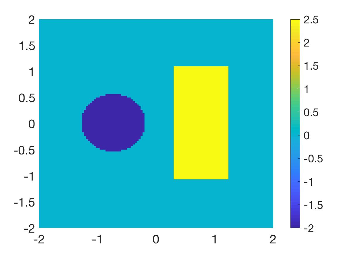
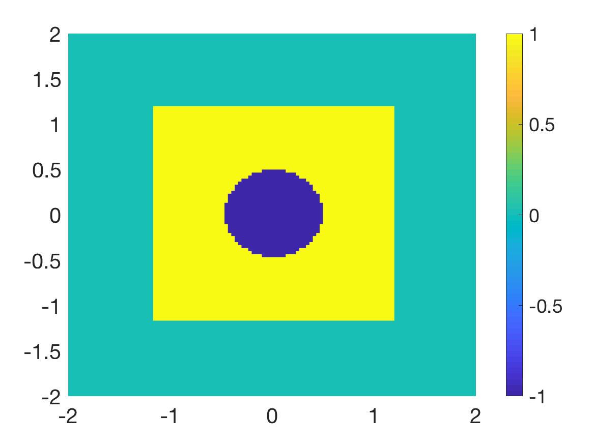
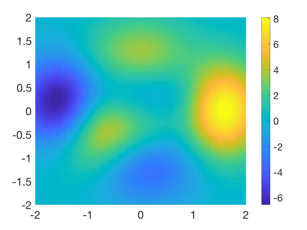
   and $g_{\mathrm{true}}(k)=\mathrm{i}k$ for $k\in[\underline{k},\overline{k}].$ We test the reconstructions of the locations, shapes and positive/negative values of the function $f$ for two different inclusions. One of them is a rectangle and the other one is a disk. In this case, the function $f_{\mathrm{true}}$ attains both positive and negative values. The numerical solution for this case is displayed on Figure 2.

   

   (a)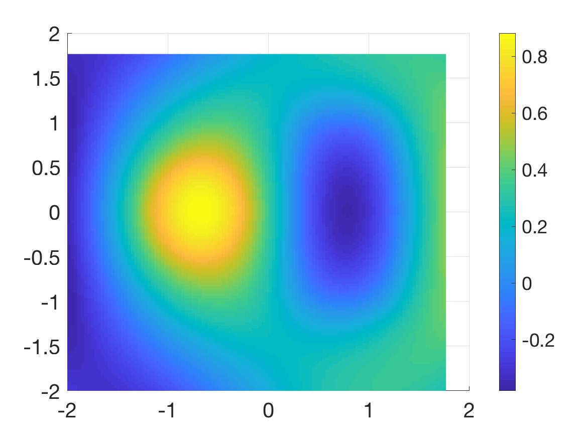

   

   (b)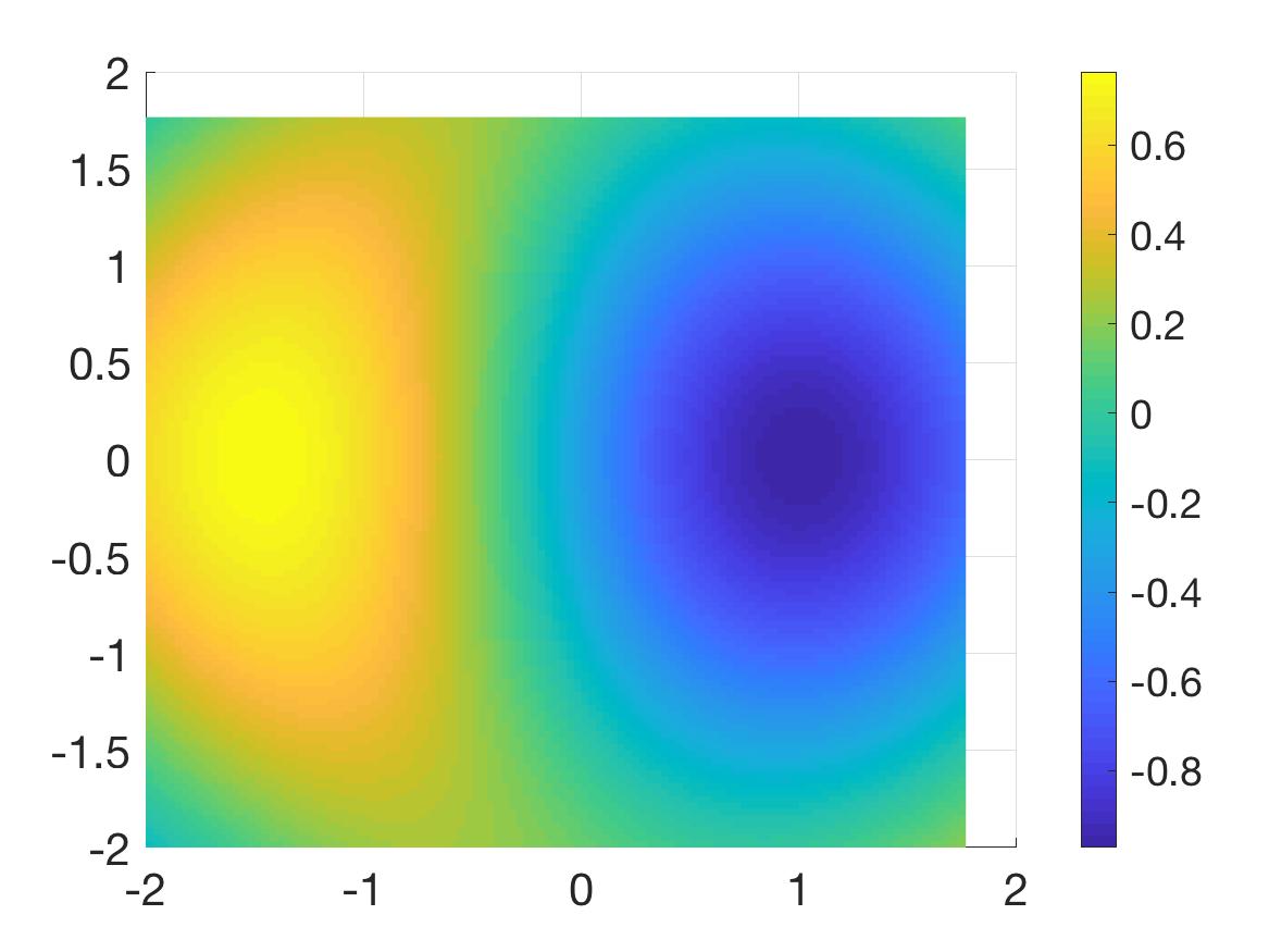

   

   (c)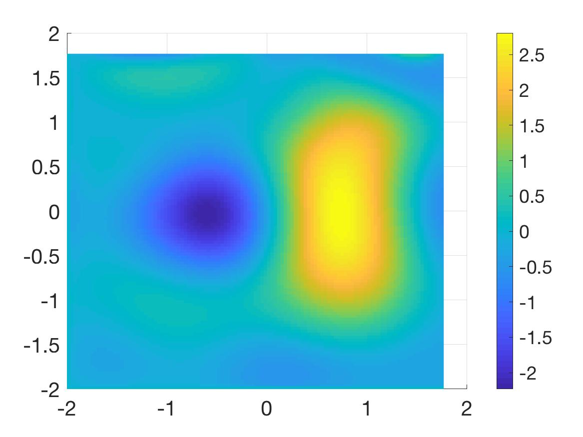

   

   (d)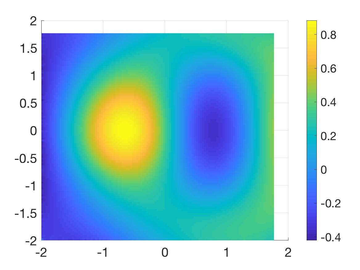

   

   (e)

   

   (f)

   Figure 2: Test 1. The true and reconstructed source functions and the true and reconstructed functions $v(\mathbf{x},k)=u(\mathbf{x},k)/g(k)$ when $k=1.5.$ The reconstructed positive value of the source function is 2.76 (relative error 10.5%). The reconstructed negative value of the source function is -2.17 (relative error 8.5%). (A) The function $f_{\rm true}$; (B) The real part of the function $v_{\rm true}(\cdot,k=1.5)$; (C) The imaginary part of the function $v_{\rm true}(\cdot,k=1.5)$; (D) The function $f_{\rm comp}$; (E) The real part of the function $v_{\rm comp}(\cdot,k=1.5)$; (F) The imaginary part of the function $v_{\rm comp}(\cdot,k=1.5)$.

   It is evident that, for this test, our method for 1.1 provides good numerical results. The reconstructed locations, shapes as well as the positive/negative values of the function  $f^{\mathrm{comp}}$ are of a good quality.

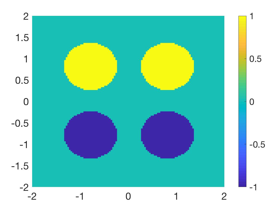
2. Test 2.Problem 1.1. Four circular inclusions. We consider the case when the function $f_{\mathrm{true}}$ is given by

   $$\begin{split}&f_{\mathrm{true}}=\left\{\begin{array}[]{rl}1,&\mbox{if}(x-0.8)^{2}+(y-0.8)^{2}<0.55^{2}\mbox{ or }(x+0.8)^{2}+(y-0.8)^{2}<0.55^{2},\\ -1,&\mbox{if}(x-0.8)^{2}+(y+0.8)^{2}<0.55^{2}\mbox{ or }(x+0.8)^{2}+(y+0.8)^{2}<0.55^{2},\\ 0,&\mbox{otherwise,}\end{array}\right.\end{split}$$

   and $g_{\mathrm{true}}(k)=1$ for all $k\in[\underline{k},\overline{k}].$ We test the model with four circular inclusions. The source function $f=1$ in the two “upper” inclusion and $f=-1$ in the two “lower” inclusions.

   The reconstruction is displayed in Figure 3. The source function is reconstructed well in the sense of locations, shapes and values.

   

   (a)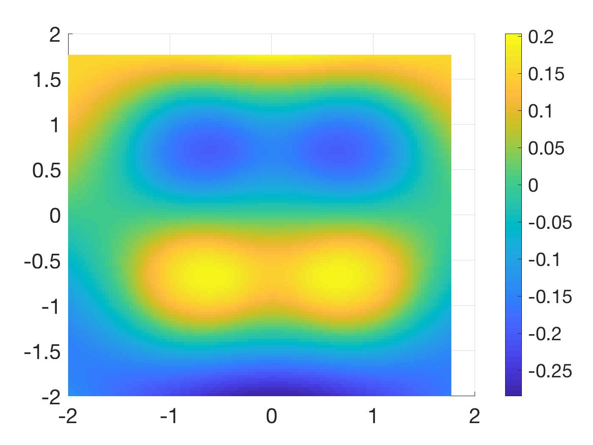

   

   (b)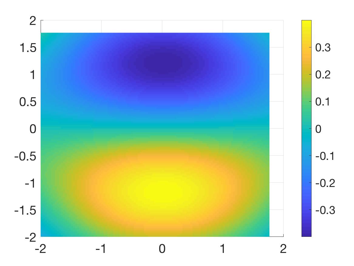

   

   (c)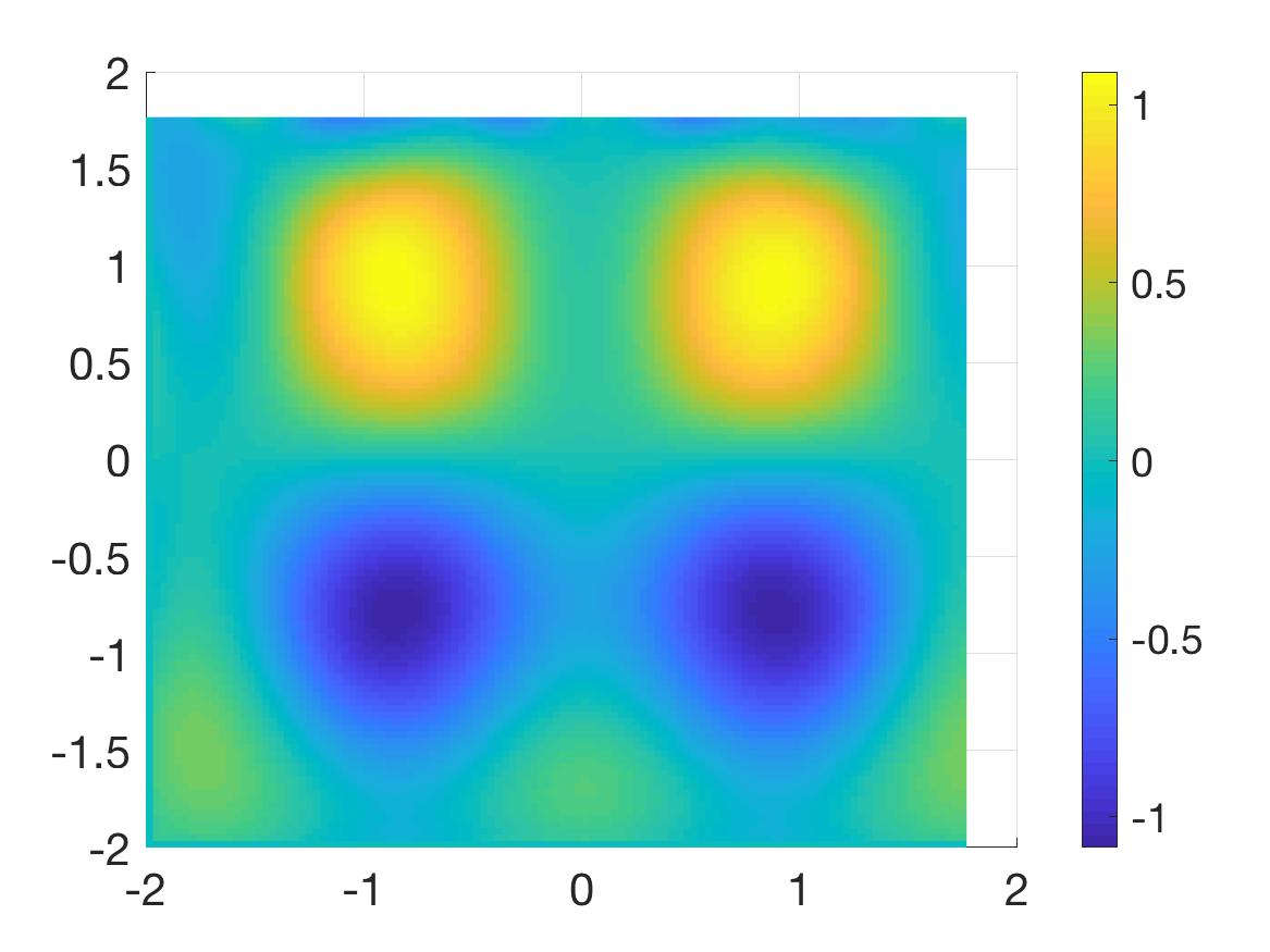

   

   (d)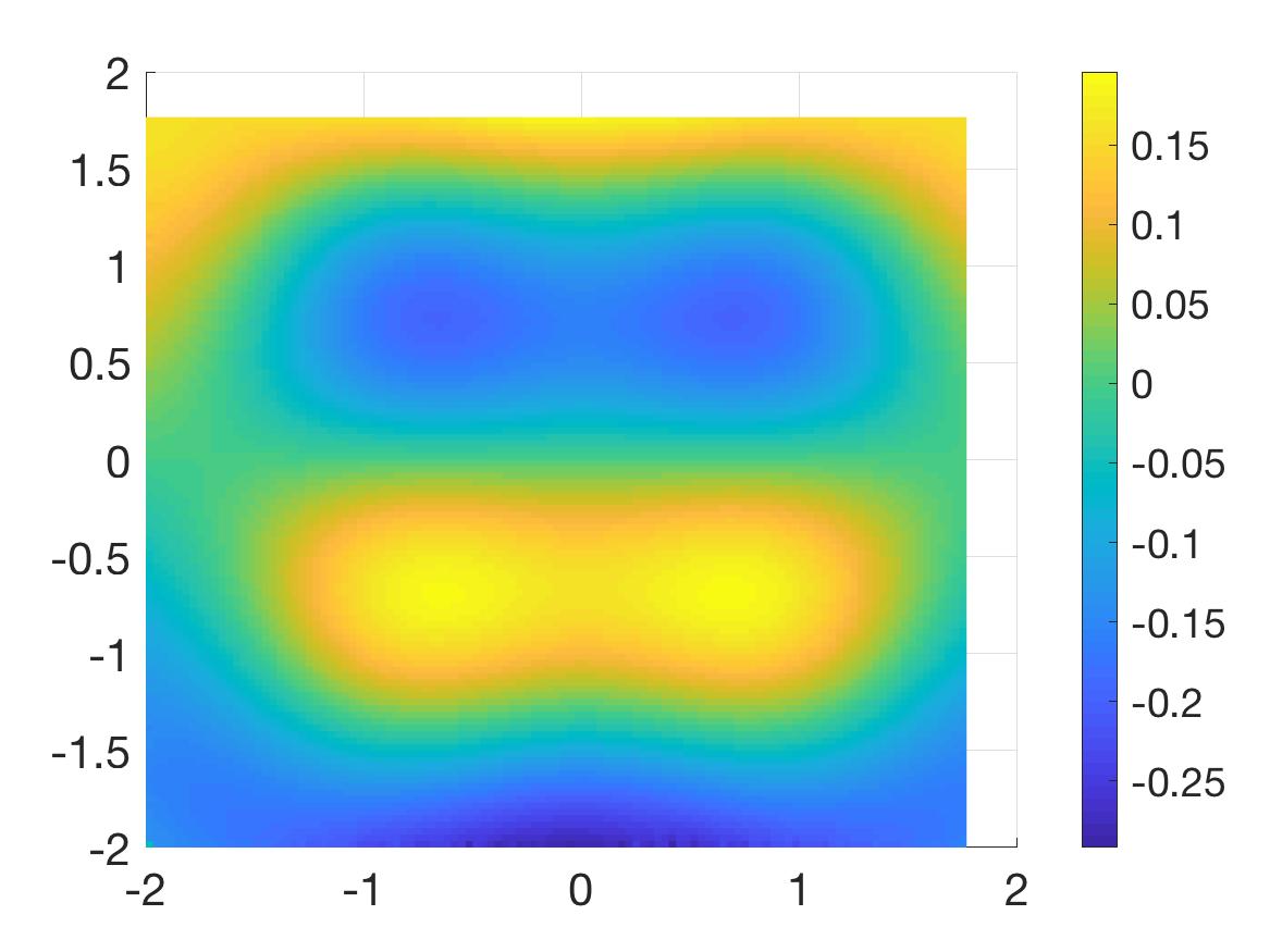

   

   (e)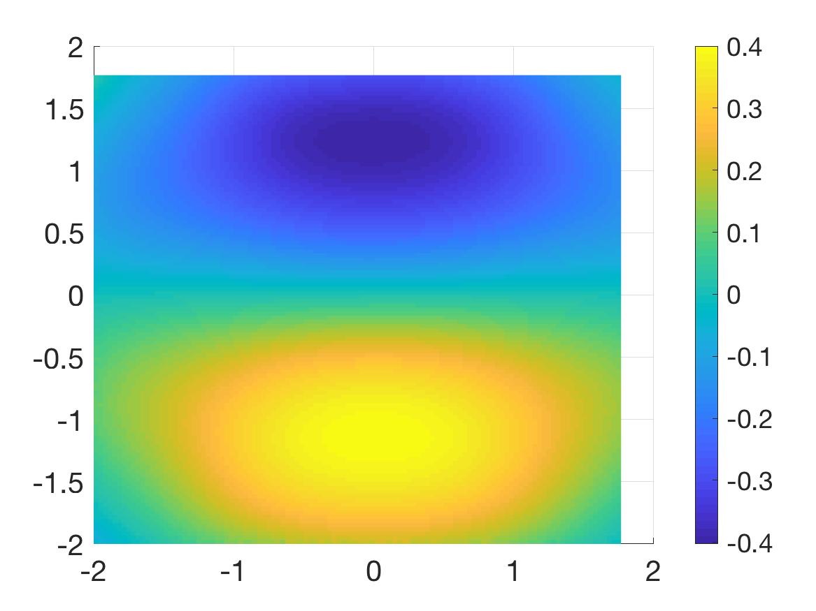

   

   (f)

   Figure 3: Test 2. The true and reconstructed source functions and the true and reconstructed functions $v(\mathbf{x},k)=u(\mathbf{x},k)/g(k)$ when $k=1.5.$ The reconstructed positive value of the source function is 1.11 (relative error 11.1%). The reconstructed negative value of the source function is -1.11 (relative error 11.1%). A) The function $f_{\rm true}$; (B) The real part of the function $v_{\rm true}(\cdot,k=1.5)$; (C) The imaginary part of the function $v_{\rm true}(\cdot,k=1.5)$; (D) The function $f_{\rm comp}$; (E) The real part of the function $v_{\rm comp}(\cdot,k=1.5)$; (F) The imaginary part of the function $v_{\rm comp}(\cdot,k=1.5)$.

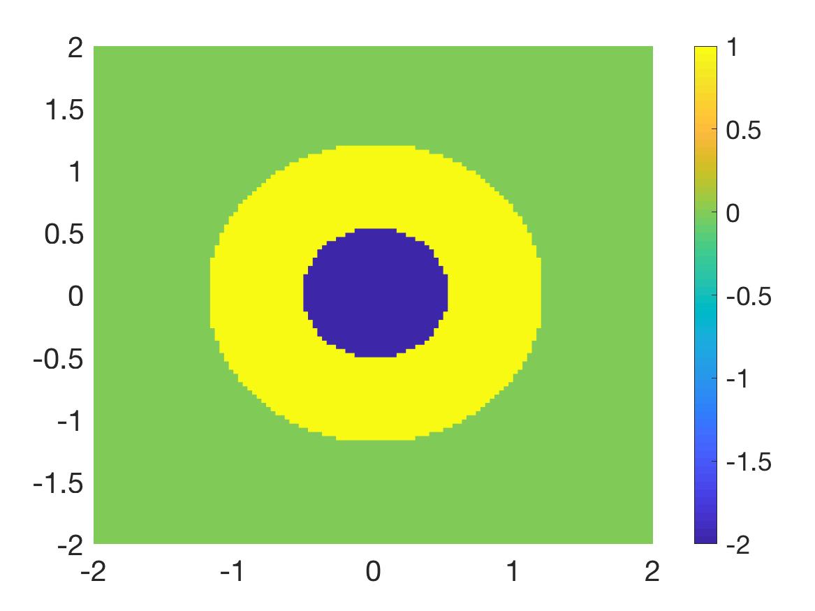
3. Test 3. Problem 1.2. A void in the square. We consider the case when the negative part of the true source function $f$ is surrounded by a square and $f$ is positive in this square. More precisely,

   $$f_{\mathrm{true}}=\left\{\begin{array}[]{rl}1&\mbox{if }\max\{|x|,|y|\}<1.2\mbox{ and }x^{2}+y^{2}\geq 0.48^{2},\\ -1&\mbox{if }x^{2}+y^{2}<0.48^{2},\\ 0&\mbox{otherwise,}\end{array}\right.$$

   and $g_{\mathrm{true}}(k)=k$ for all $k\in[\underline{k},\overline{k}].$

   

   (a)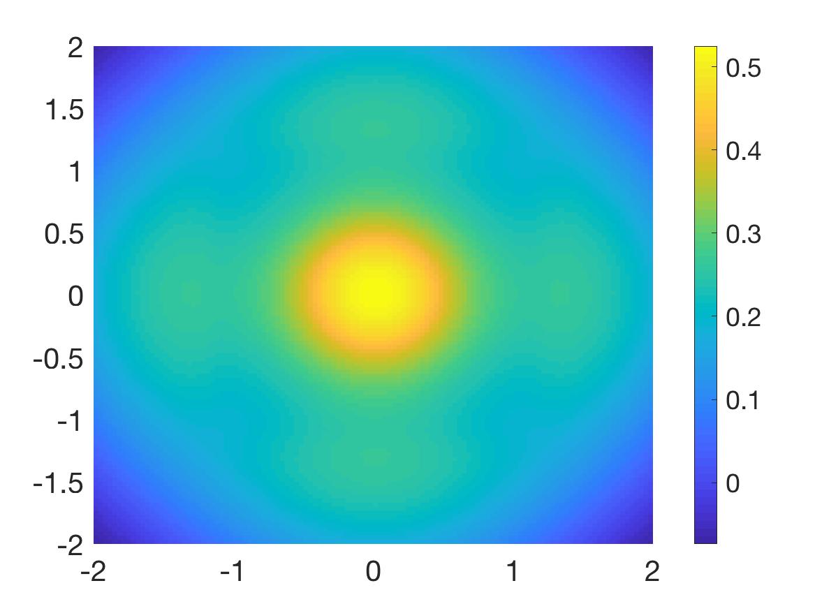

   

   (b)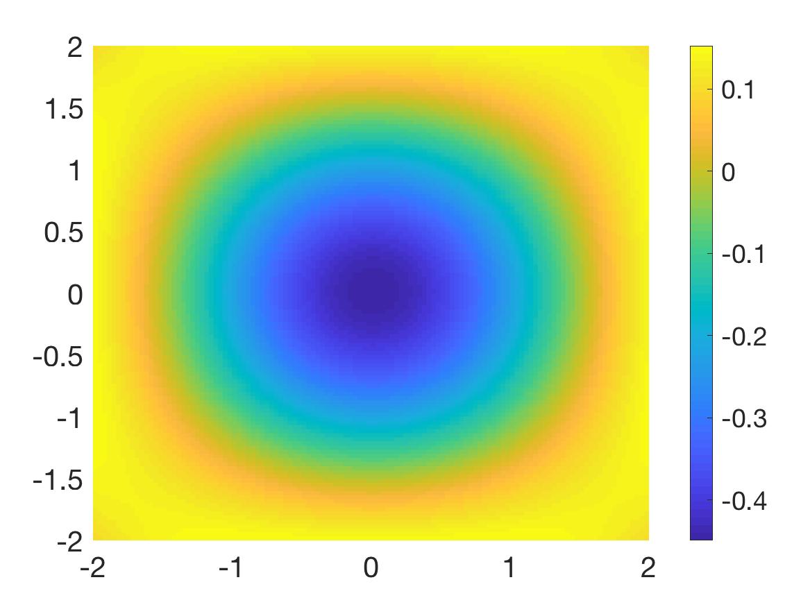

   

   (c)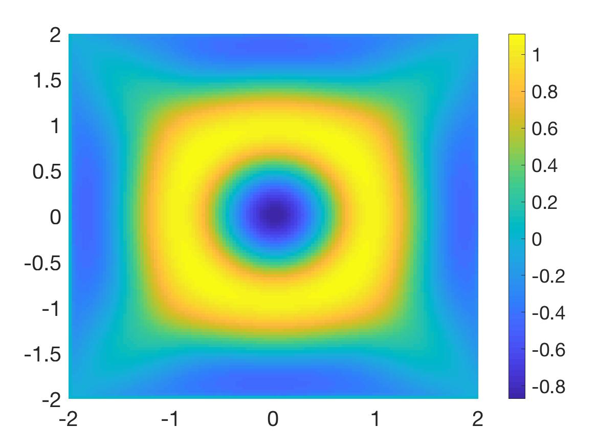

   

   (d)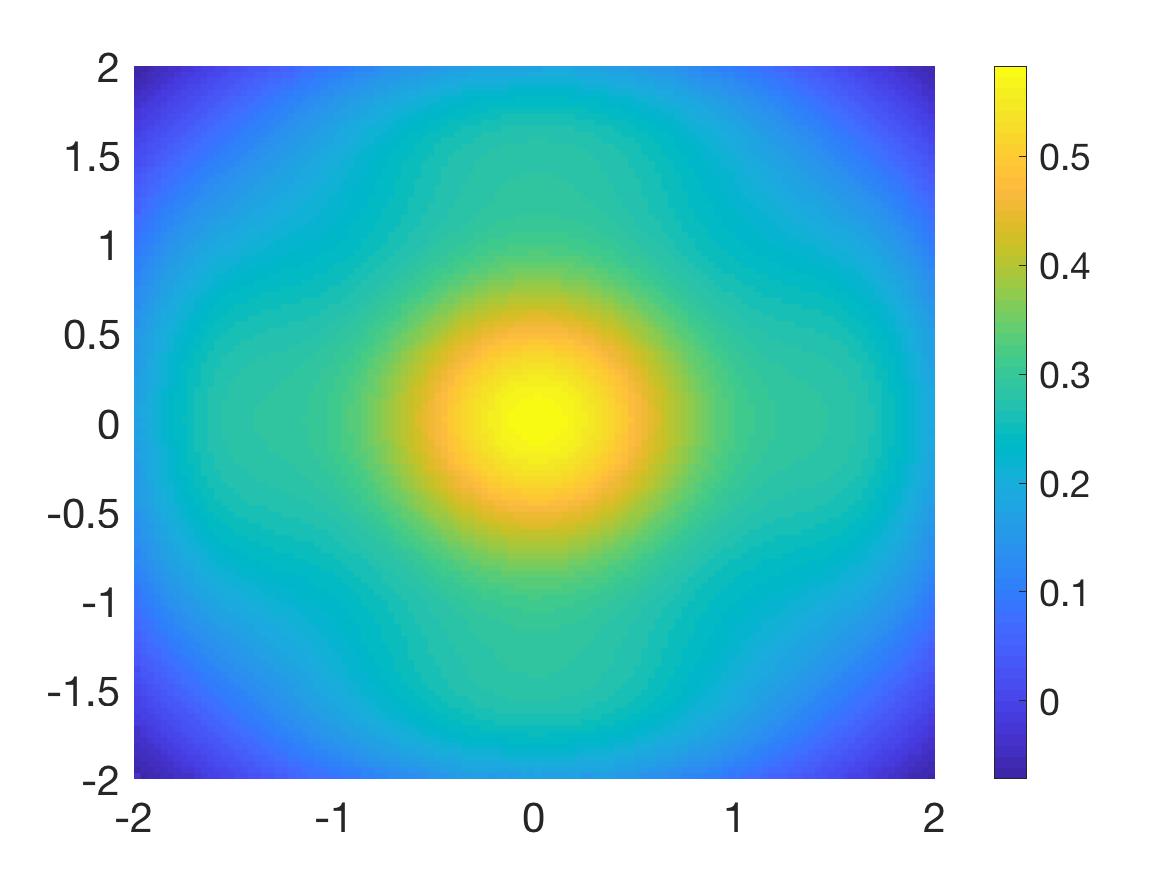

   

   (e)

   

   (f)

   Figure 4: Test 3. The true and reconstructed source functions and the true and reconstructed functions $v(\mathbf{x},k)=u(\mathbf{x},k)/g(k)$ when $k=1.5.$ The reconstructed positive value of the source function is 1.09 (relative error 9.0%). The reconstructed negative value of the source function is -0.89 (relative error 11.0%). A) The function $f_{\rm true}$; (B) The real part of the function $v_{\rm true}(\cdot,k=1.5)$; (C) The imaginary part of the function $v_{\rm true}(\cdot,k=1.5)$; (D) The function $f_{\rm comp}$; (E) The real part of the function $v_{\rm comp}(\cdot,k=1.5)$; (F) The imaginary part of the function $v_{\rm comp}(\cdot,k=1.5)$.

   The true $f_{\text{true}}$ and computed $f^{\text{comp}}$ source functions are displayed in Figure 4. We can see computed shapes of the “positive” square and the “negative” disk are quite acceptable. Given that the noise in the data is 5%, errors in values of the function $f^{\text{comp}}$ are also acceptable.

4. Test 4. Problem 1.2. Ring. We consider a model that is similar to that in the previous test. The main difference is the “outer positive” part of the true source function is a ring rather than a square. The function $f_{\mathrm{true}}$ is

   $$f_{\mathrm{true}}=\left\{\begin{array}[]{rl}1&\mbox{if }0.52^{2}<x^{2}+y^{2}<1.2^{2},\\ -2&\mbox{if }x^{2}+y^{2}\leq 0.52^{2},\\ 0&\mbox{otherwise,}\end{array}\right.$$ (6.16)

   and $g_{\mathrm{true}}(k)=k^{2}$ for all $k\in[\underline{k},\overline{k}].$

   

   (a)

   

   (b)

   

   (c)

   

   (d)

   

   (e)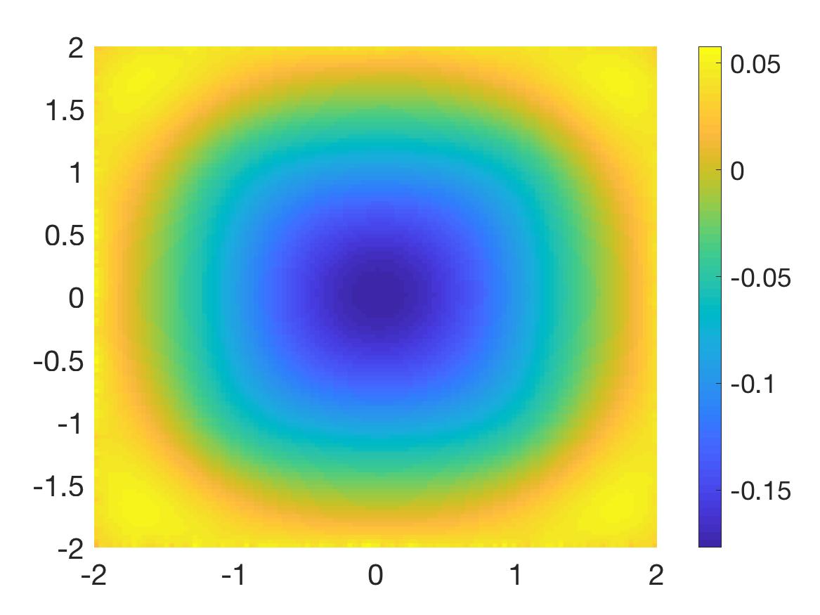

   

   (f)

   Figure 5: Test 4. The true and reconstructed source functions and the true and reconstructed functions $v(\mathbf{x},k)=u(\mathbf{x},k)/g(k)$ when $k=1.5.$ The reconstructed positive value of the source function is 1.12 (relative error 12.0%). The reconstructed negative value of the source function is -1.94 (relative error 3.0%). A) The function $f_{\rm true}$; (B) The real part of the function $v_{\rm true}(\cdot,k=1.5)$; (C) The imaginary part of the function $v_{\rm true}(\cdot,k=1.5)$; (D) The function $f_{\rm comp}$; (E) The real part of the function $v_{\rm comp}(\cdot,k=1.5)$; (F) The imaginary part of the function $v_{\rm comp}(\cdot,k=1.5)$.

   In Figure 5, one can see that the source function is computed rather accurately. The values of both “positive” and “negative” parts of the inclusion are computed with a good accuracy.

5. Test 5. 1.2. Continuous surface. We take for $\left(x,y\right)\in\Omega$

   $$f_{\mathrm{true}}=3(1-x)^{2}e^{-x^{2}}-(y+1)^{2}-10(x/5-x^{3}-y^{5})e^{-x^{2}-y^{2}}-1/3e^{-(x+1)^{2}-y^{2}},$$

   which is the function “peaks” built-in Matlab, restricted on $\Omega$. This function is interesting since its support is not compactly contained in $\Omega$ and its graph behaves as a surface rather than the “inclusion” from the previous tests. We set $g_{\mathrm{true}}(k)=\sin(k)+2$ for all $k\in[\underline{k},\overline{k}].$

   

   (a)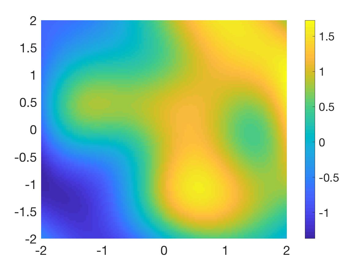

   

   (b)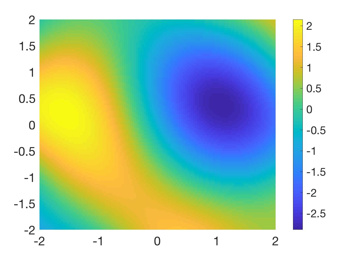

   

   (c)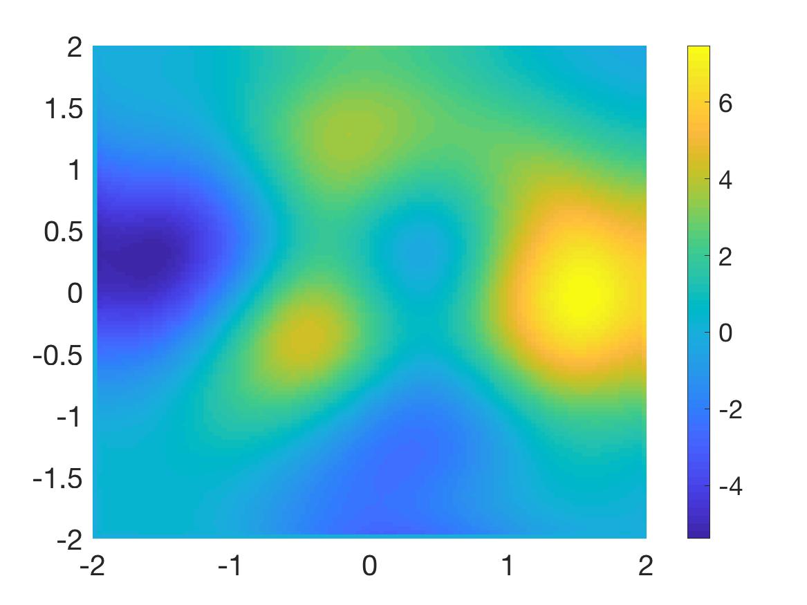

   

   (d)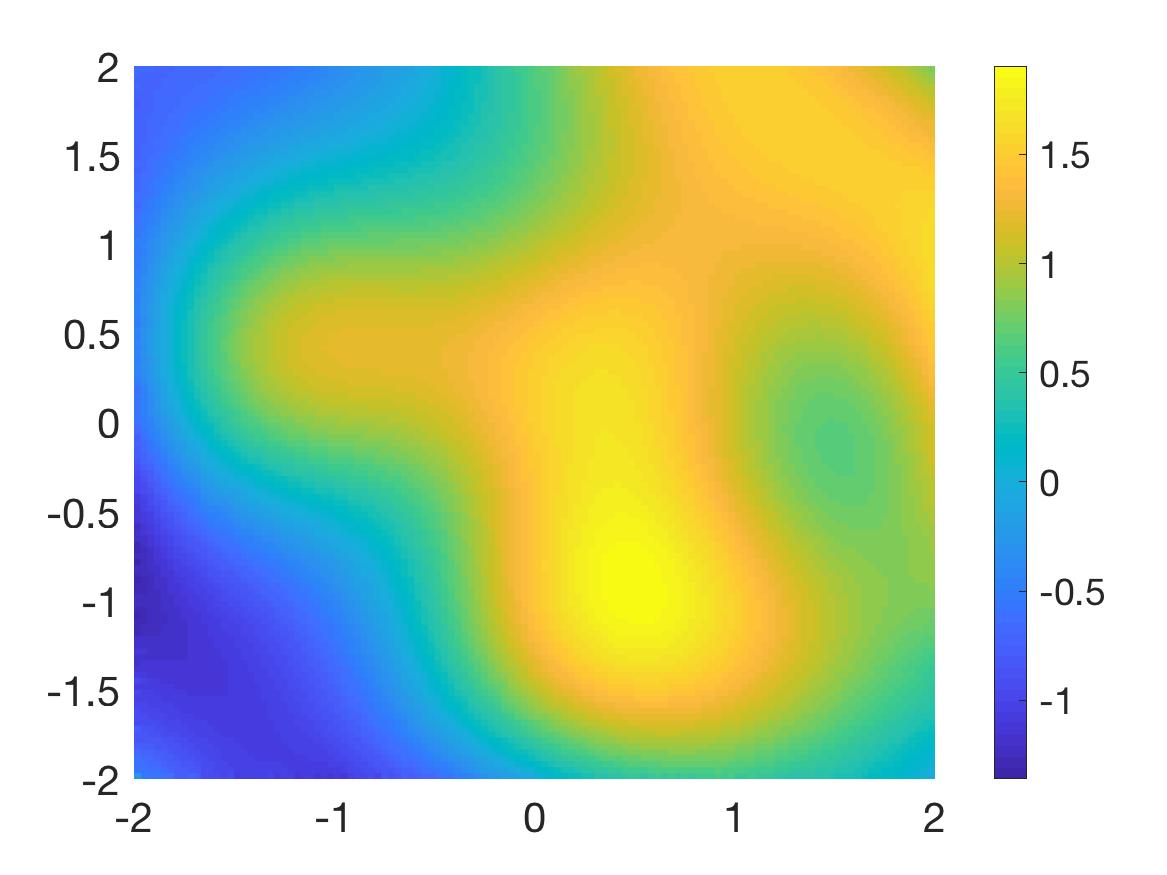

   

   (e)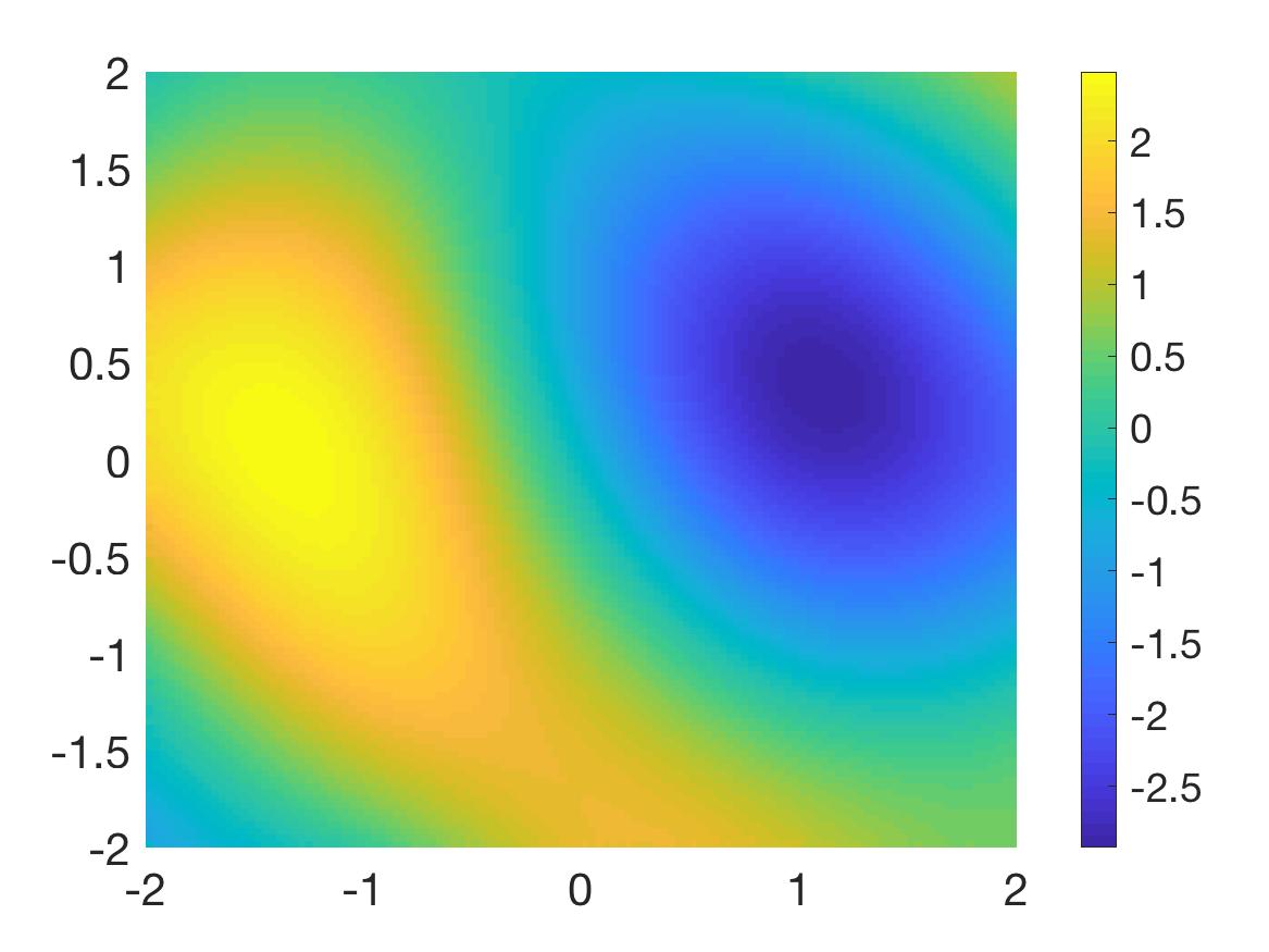

   

   (f)

   Figure 6: Test 5. The true and reconstructed source functions and the true and reconstructed functions $v(\mathbf{x},k)=u(\mathbf{x},k)/g(k)$ when $k=1.5.$ The true and reconstructed maximal positive value of the source function are 8.10 and 7.36 (relative error 9.1%) respectively. The true and reconstructed minimal negative value of the source function are -6.55 and -5.48 (relative error 16.0%) respectively. A) The function $f_{\rm true}$; (B) The real part of the function $v_{\rm true}(\cdot,k=1.5)$; (C) The imaginary part of the function $v_{\rm true}(\cdot,k=1.5)$; (D) The function $f_{\rm comp}$; (E) The real part of the function $v_{\rm comp}(\cdot,k=1.5)$; (F) The imaginary part of the function $v_{\rm comp}(\cdot,k=1.5)$.

The numerical results for this test are displayed in Figure 6. It is evident that our method works well for this interesting case.

References

- [1] R. Albanese and P. Monk, The inverse source problem for Maxwell’s equations, Inverse Problems, 22 (2006), 1023–1035.
- [2] H. Ammari, G. Bao and J. Flemming, An inverse source problem for Maxwell’s equations in magnetoencephalography, SIAM J. Appl. Math., 62 (2002), 1369–1382.
- [3] G. Bao, J. Lin and F. Triki, A multi-frequency inverse source problem, Journal of Differential Equations, 249 (2010), 3443–3465.
- [4] G. Bao, J. Lin and F. Triki, An inverse source problem with multiple frequency data, C. R. Math., 349 (2011), 855–9.
- [5] G. Bao, J. Lin and F. Triki, Numerical solution of the inverse source problem for the Helmholtz equation with multiple frequency data, Contemp. Math, 548 (2011), 45–60.
- [6] E. Bécache, L. Bourgeois, L. Franceschini and J. Dardé, Application of mixed formulations of quasi-reversibility to solve ill-posed problems for heat and wave equations: The 1d case, Inverse Problems & Imaging, 9 (2015), 971–1002.
- [7] L. Beilina and M. V. Klibanov, Approximate Global Convergence and Adaptivity for Coefficient Inverse Problems, Springer, New York, 2012.
- [8] M. Bellassoued and M. Yamamoto, Carleman Estimates and Applications to Inverse Problems for Hyperbolic Systems, Springer, Japan, 2017.
- [9] L. Bourgeois, Convergence rates for the quasi-reversibility method to solve the Cauchy problem for Laplace’s equation, Inverse Problems, 22 (2006), 413–430.
- [10] L. Bourgeois and J. Dardé, A duality-based method of quasi-reversibility to solve the Cauchy problem in the presence of noisy data, Inverse Problems, 26 (2010), 095016.
- [11] L. Bourgeois, D. Ponomarev and J. Dardé, An inverse obstacle problem for the wave equation in a finite time domain, Inverse Probl. Imaging, 13 (2019), 377–400.
- [12] A. L. Bukhgeim and M. V. Klibanov, Uniqueness in the large of a class of multidimensional inverse problems, Soviet Math. Doklady, 17 (1981), 244–247.
- [13] X. Cao and H. Liu, Determining a fractional Helmholtz system with unknown source and medium parameter determining a fractional Helmholtz system with unknown source and medium parameter, preprint, arXiv:1803.09538v1.
- [14] J. Cheng, V. Isakov and S. Lu, Increasing stability in the inverse source problem with many frequencies, Journal of Differential Equations, 260 (2016), 4786–4804.
- [15] C. Clason and M. V. Klibanov, The quasi-reversibility method for thermoacoustic tomography in a heterogeneous medium, SIAM J. Sci. Comput., 30 (2007), 1–23.
- [16] D. Colton and R. Kress, Inverse acoustic and electromagnetic scattering theory. Applied Mathematical Sciences, 3rd edition, Springer, New York, 2013.
- [17] J. Dardé, Iterated quasi-reversibility method applied to elliptic and parabolic data completion problems, Inverse Problems and Imaging, 10 (2016), 379–407.
- [18] G. Dassios and F. Kariotou, Magnetoencephalography in ellipsoidal geometry, J. Math. Physics, 44 (2003), 220–241.
- [19] A. El Badia and T. Ha-Duong, An inverse source problem in potential analysis, Inverse Problems, 16 (2000), 651–663.
- [20] M. N. Entekhabi and V. Isakov, On increasing stability in the two dimensional inverse source scattering problem with many frequencies, Inverse Problems, 34 (2018), 055005.
- [21] S. He and V. G. Romanov, Identification of dipole sources in a bounded domain for Maxwell’s equations, Wave Motion, 28 (1998), 25–44.
- [22] V. Isakov and S. Lu, Increasing stability in the inverse source problem with attenuation and many frequencies, SIAM J. Appl. Math., 78 (2018), 1–18.
- [23] V. Isakov and S. Lu, Inverse source problems without (pseudo) convexity assumptions, Inverse Probl. Imaging, 12 (2018), 955–970.
- [24] S. I. Kabanikhin, K. K. Sabelfeld, N. S. Novikov and M. A. Shishlenin, Numerical solution of the multidimensional Gelfand-Levitan equation, J. Inverse and Ill-Posed Problems, 23 (2015), 439–450.
- [25] S. I. Kabanikhin, A. D. Satybaev and M. A. Shishlenin, Direct Methods of Solving Inverse Hyperbolic Problems, VSP, Utrecht, 2005.
- [26] S. I. Kabanikhin and M. A. Shishlenin, Numerical algorithm for two-dimensional inverse acoustic problem based on Gel’fand–Levitan–Krein equation, Journal of Inverse and Ill-posed Problems, 18 (2011), 979–995.
- [27] B. Kaltenbacher and W. Rundell, Regularization of a backwards parabolic equation by fractional operators, Inverse Probl. Imaging, 13 (2019), 401–430.
- [28] M. V. Klibanov, Carleman estimates for global uniqueness, stability and numerical methods for coefficient inverse problems, J. Inverse and Ill-Posed Problems, 21 (2013), 477–560.
- [29] M. V. Klibanov, Carleman estimates for the regularization of ill-posed Cauchy problems, Applied Numerical Mathematics, 94 (2015), 46–74.
- [30] M. V. Klibanov, Convexification of restricted Dirichlet to Neumann map, J. Inverse and Ill-Posed Problems, 25 (2017), 669–685.
- [31] M. V. Klibanov, A. E. Kolesov, L. Nguyen and A. Sullivan, A new version of the convexification method for a 1-D coefficient inverse problem with experimental data, Inverse Problems, 34 (2018), 35005.
- [32] M. V. Klibanov, J. Li and W. Zhang, Convexification of electrical impedance tomography with restricted Dirichlet-to-Neumann map data, Inverse Problems, 35 (2019), 035005.
- [33] M. V. Klibanov and L. H. Nguyen, PDE-based numerical method for a limited angle X-ray tomography, Inverse Problems, 35 (2019), 045009.
- [34] M. V. Klibanov and F. Santosa, A computational quasi-reversibility method for Cauchy problems for Laplace’s equation, SIAM J. Appl. Math., 51 (1991), 1653–1675.
- [35] M. V. Klibanov and A. Timonov, Carleman Estimates for Coefficient Inverse Problems and Numerical Applications, Inverse and Ill-Posed Problems Series, VSP, Utrecht, 2004.
- [36] M. V. Klibanov and N. T. Thành, Recovering of dielectric constants of explosives via a globally strictly convex cost functional, SIAM J. Appl. Math., 75 (2015), 518–537.
- [37] R. Lattès and J. L. Lions, The Method of Quasireversibility: Applications to Partial Differential Equations, Elsevier, New York, 1969.
- [38] J. Li, H. Liu and H. Sun, On a gesture-computing technique using eletromagnetic waves, Inverse Probl. Imaging, 12 (2018), 677–696.
- [39] H. Liu and G. Uhlmann, Determining both sound speed and internal source in thermo- and photo-acoustic tomography, Inverse Problems, 31 (2015), 105005.
- [40] L. H. Nguyen, An inverse space-dependent source problem for hyperbolic equations and the Lipschitz-like convergence of the quasi-reversibility method, Inverse Problems, 35 (2019), 035007.
- [41] A. N. Tikhonov, A. Goncharsky, V. V. Stepanov and A. G. Yagola, Numerical Methods for the Solution of Ill-Posed Problems, Kluwer Academic Publishers Group, Dordrecht, 1995.
- [42] G. Wang, F. Ma, Y. Guo and J. Li, Solving the multi-frequency electromagnetic inverse source problem by the Fourier method, J. Differential Equations, 265 (2018), 417–443.
- [43] X. Wang, Y. Guo, J. Li and H. Liu, Mathematical design of a novel input/instruction device using a moving acoustic emitter, Inverse Problems, 33 (2017), 105009.
- [44] X. Wang, Y. Guo, D. Zhang and H. Liu, Fourier method for recovering acoustic sources from multi-frequency far-field data, Inverse Problems, 33 (2017), 035001.
- [45] X. Wang, S. M., Y. Guo, H. Li and H. Liu, Fourier method for identifying electromagnetic sources with multi-frequency far-field data, to appear on Journal of Computational and Applied Mathematics, DOI: 10.1016/j.cam.2019.03.013.
- [46] X. Xiang and H. Sun, Sparse reconstructions of acoustic source for inverse scattering problems in measure space, to appear on Inverse Problems.
- [47] D. Zhang and Y. Guo, Fourier method for solving the multi-frequency inverse source problem for the Helmholtz equation, Inverse Problems, 31 (2015), 035007.
- [48] D. Zhang, Y. Guo, J. Li and H. Liu, Retrieval of acoustic sources from multi-frequency phaseless data, Inverse Problems, 34 (2018), 094001.