Numerical Methods for Biomembranes:
conforming subdivision methods
versus non-conforming PL methods
Revised: March 11, 2020)
Abstract:
The Canham-Helfrich-Evans models of biomembranes consist of a family of geometric constrained variational problems. In this article, we compare two classes of numerical methods for these variational problems based on piecewise linear (PL) and subdivision surfaces (SS). Since SS methods are based on spline approximation and can be viewed as higher order versions of PL methods, one may expect that the only difference between the two methods is in the accuracy order. In this paper, we prove that a numerical method based on minimizing any one of the ‘PL Willmore energies’ proposed in the literature would fail to converge to a solution of the continuous problem, whereas a method based on minimization of the bona fide Willmore energy, well-defined for SS but not PL surfaces, succeeds. Motivated by this analysis, we propose also a regularization method for the PL method based on techniques from conformal geometry. We address a number of implementation issues crucial for the efficiency of our solver. A software package called Wmincon accompanies this article, provides parallel implementations of all the relevant geometric functionals. When combined with a standard constrained optimization solver, the geometric variational problems can then be solved numerically. To this end, we realize that some of the available optimization algorithms/solvers are capable of preserving symmetry, while others manage to break symmetry; we explore the consequences of this observation.
Acknowledgments. TY is indebted to Tom Duchamp and Aaron Yip for extensive discussions and many of their insightful remarks. We also thank Tim Mitchell, Michael Overton, Justin Smith, and Shawn Walker for help. TY was partially supported by NSF grants DMS 0915068 and DMS 1115915. RK was supported in part by the Aspen Center For Physics (funded by NSF-PHY 1607611), ICERM (funded by NSF-DMS 1439786), and MSRI (funded by NSF-DMS 1440140.)
Keywords: Lipid bilayer, Canham-Evans-Helfrich model, Willmore energy, Willmore surfaces, Conforming & non-conforming finite element methods, Subdivision surface, PL surface, Discrete differential geometry, Conformal parametrization, Nonlinear optimization, Symmetry preserving, Symmetry breaking.
1 Introduction
Lipid bilayers are arguably the most elementary and indispensable structural components of biological membranes which form the boundary of all cells. It is known since the seminal work of Canham [14], Helfrich [39] and Evans [30] in the 70’s that bending elasticity, induced by curvature, plays the key role in driving the geometric configurations of such membranes.
The so-called spontaneous curvature model of Helfrich suggests that a biomembrane surface configures itself to minimize subject to the area, volume and area difference (related to the bilayer characteristics) constraints, i.e. solves the variational Helfrich problem
| (1.1) |
Here is the mean curvature. In (ii), is the enclosed volume, expressed here as a surface integral of via the divergence theorem. The connection of (iii) to bilayer area difference comes from the relation , where and are the ‘-offset surfaces’,111We assume that the normal of any closed orientable surface points outward. In particular, it means for a sphere. and that the thickness of the lipid bilayer, , is negligible compared to the size of the vesicle; see Figure 1. The constraint values , and are determined by physical conditions (e.g. temperature, concentration). is called the Willmore energy of the surface . When the area-difference constraint (iii) is omitted, the variational problem is referred to as the Canham problem. When even the volume constraint (ii) is omitted, there is essential no constraint as is scale-invariant; in this case the area constraint (i) only fixes the scale, and we refer to the variational problem as the Willmore problem.
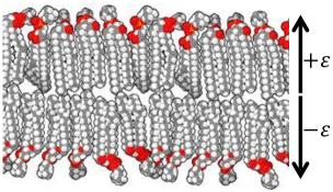
Due to the scale-invariance of the Willmore energy, the solution, up to homothety, of any of the Willmore, Canham or Helfrich problems depends only on the reduced volume and reduced total mean curvature defined by:
| (1.2) |
This terminology is used by a group of biophysicists who have done many computational and physical experiments exploring the shapes of phospholipid vesicles, and we shall follow it. Note that is essentially what a geometer would call the isoperimetric ratio. By the isoperimetric inequality, we have and is uniquely realized by a round sphere.
It is observed experimentally that no topological change occurs in any accessible time-scale, so we aim to solve any of the Helfrich, Canham or Willmore problems when is assumed to be an orientable closed surface with a fixed genus . Spherical () vesicles are the most common among naturally occurring biomembranes, although higher genus ones have been synthesized in the laboratory [56, 43, 66]. The Canham, Helfrich and related models explain the large variety of shapes observed in even a closed vesicle with a spherical topology [51, 66, 50, 75].
Several numerical treatments of these models have been proposed in the literature: [40, 10], [32, 15], [9, 19], [22, 21, 23], [63]. Among these, the methods in [40, 10] were used extensively by biophysicists to study real lipid bilayer membranes. While the key ingredients of these algorithms are implemented in Brakke’s well-known Surface Evolver software [10], the overall algorithms were not completely analyzed by the geometers who invented them [40, 10, 33] and even less so by the biophysicists who used them [43, 56, 66, 75]. As such, there are little understanding of these methods, and the computational results claimed in the extensive biophysics literature are difficult to reproduce. Moreover, there is no systematic comparison of this method with the later ones, at both a theoretical or computational level.
These numerical methods continue to be used extensively in the study of phenomena in biomembranes, see, e.g. [78, 4, 44, 45, 2] and references therein. Similar geometric variational problems show up in other scientific areas. A notable example is found in the quasi-local mass problem of general relativity, in which maximizers of the Hawking mass – defined similarly as the Willmore energy – are sought.
The goal of this paper is to clarify and refine some of these numerical methods, and establish some theoretical understandings of them. Before we proceed, we mention further related work on discrete minimal surfaces and discrete elasticae (the 1-D counterpart to Willmore surface), see, e.g., [25, 26, 64, 13, 62] and the references therein.
1.1 PL and SS
A standard approach to represent surfaces of arbitrary topology is to use the piecewise linear (PL) approach. A PL surface can be specified by a mesh where records the 3-D coordinates of the vertices of the control mesh, denotes the total number of vertices, and is a list of triplets of indices from which records the vertices of each of the triangle faces in the mesh . We assume that the PL surfaces realized by the mesh are closed and orientable. The orientation can be conveniently encoded in a consistent ordering of the vertices in the face list .
In a numerical method, is usually fixed and varies. This fits the framework of our variational problems well, as fixing also fixes the genus of the surface, and varying means we find the embedding of – viewed as an abstract simplicial complex – that optimizes the Willmore energy under the corresponding constraint(s).
A closed, oriented PL surface has a well-defined area and enclosed volume , but no classically defined normals or mean curvatures, hence it also does not have a classically defined total mean curvature or Willmore energy . As such, any numerical method for the Willmore, Canham, or Helfrich problems based on approximating the solution surfaces by PL surfaces may be classified as a nonconforming method in FEM parlance.
A subdivision surface (SS) is specified by the same data , except that the associated surface has enough regularity for a well-defined total mean curvature or Willmore energy . We shall primarily be using the Loop and C2g0 subdivision surfaces introduced in [52] and [15], respectively. See Figure 2(a) for a genus 0 control mesh, and Figure 2(b) for the corresponding Loop subdivision surface. For each face in , there is a corresponding surface patch; see Figure 2(b).
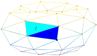
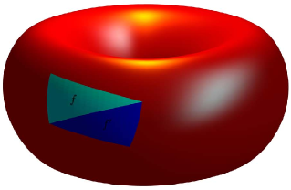
The C2g0 scheme handles only genus 0 and 1 surfaces using control meshes with only valence 3 and 6 vertices; the resulting SS are everywhere, so there is no question about the well-definedness of and . The Loop subdivision scheme handles surface of arbitrary genus and control meshes with arbitrary valences, but the resulting SS are not everywhere. They are however regular enough to have well-defined and . (The subdivision functions are in when expressed in characteristic coordinates; see Section 3.1.) Therefore, any numerical method for the Willmore, Canham, or Helfrich problems based on approximating the solution surfaces by SS may be classified as a conforming method.
1.2 Contributions of this paper
This paper contributes to the numerical study of biomembranes in the following ways:
-
(I)
In Section 2, we give an exposition of numerical methods based on both PL and SS. In the PL case, we connect and compare several different ideas developed in the applied geometry literature [40, 10, 7, 55, 20]. In the SS case, we explain how all the functionals and their gradients with respect to control vertex coordinates can be efficiently computed based on a precomputation of basis functions. In both cases, we develop parallel implementations and explore new examples. A Matlab based toolbox named Wmincon, with CUDA and C++ implementations of all key functionals, is available online, at
for reproducing the computational results. These algorithmic developments allow us to use the SS method to attack many instances of the Willmore, Canham and Helfrich problems that would otherwise be too slow, if not impossible, to solve on existing computers.
-
(II)
In Section 3, we present an argument explaining why a conforming method would work. This result relies on the existence theory of Willmore minimizers pioneered by Simon [67]. In contrast, we show that a naive minimization of several PL Willmore energies would fail to solve the Willmore problem. The analysis elucidates the difference between conforming and non-conforming methods.
-
(III)
In Section 4, based on a well-founded principle (Section 4.1) exploiting the uniformization theorem and the theory of harmonic maps, we propose a regularization of the PL methods based on penalization by harmonic energy. Unlike the unregularized PL methods which are doomed to fail, the regularized method appears to yield solutions converging to those of the continuous problems.
-
(IV)
In Section 5, we make the observation that certain optimization algorithms are capable of preserving symmetry, while others are capable of breaking symmetries. We carry out a number of experiments comparing different optimization algorithms in conjunction with our discretization methods. The experiments reveal subtle analytic properties of the optimization problems arising from the SS methods. We formulate a number of conjectures.
The kind of conforming and non-conforming methods we study in this article are those in the spirit of ‘minimizing a discretization’, i.e. the methods under study first discretize the variational problem, in either a conforming or non-conforming way, followed by solving the resulting finite-dimensional optimization problem. There are methods, such as those in [9, 63], that are in the spirit of ‘discretizing a minimization’. These methods first consider a minimization process in the continuous setting, akin to a gradient flow, followed by strategies to discretize the flow. This last step can also be done in a conforming or non-conforming way. These methods are all based on explicit representations of surfaces; there are also methods based on implicit representations, such as the phase field methods of Du et al [22, 21, 23].
2 Numerical Methods Based on PL and SS Functionals
Recall that either a PL or SS is specified by a control mesh . In our numerical method, we assume that is fixed and varies. For most , an immersed surface, denoted by , is defined. The numerical methods considered here approximate the Helfrich problem (1.1) by a finite-dimensional analog:
| (2.1) |
The numerical methods for the Canham and Willmore problems are similar: simply drop the corresponding constraints. Already mentioned in Section 1.1, the PL and SS methods have the following features and relative pros and cons:
-
•
For SS (based on any regular enough scheme, such as Loop and C2g0), all four functionals are the exact, well-defined, values of the , , and of the corresponding subdivision surface. Their computations, however, have to be performed based on numerical integration.
-
•
For PL, and are not well-defined for the corresponding PL surface. We will therefore replace and in (2.1) by a certain consistent discretization, to be reviewed below. These PL Willmore and total mean curvature energies are relatively simple to implement and no numerical integration is required.
The materials in this section are mostly not new, some of them are actually quite old. The intention is to unify them at one place in order to prepare us for the later sections.
At first glance, one may expect that the PL method is simply less accurate than the SS methods, i.e. a PL method would converge but at a lower rate compared to a SS method. Our analysis in Section 3 falsifies this speculation. A bulk of this section discusses the definition, properties and computation of these functionals and their gradients. Efficient computation of these functionals and their gradients are necessary for the numerical solution of the Helfrich, Canham and Willmore problems using a standard nonlinear optimization solver; see Section 2.3.
2.1 , , , for PL surfaces
The area and enclosed volume are of course part of the biomembrane problems. Their gradients are not only needed for our optimization solver but also are connected to the way and are defined and computed. For these reasons, we derive them for the convenience of the readers.
We aim to clarify some not so well-documented details in the literature, such as the sign issue of discrete mean curvature, which is irrelevant for but crucial for , and the choice of local areas, which is irrelevant for but impact the behavior for . Another goal is to elucidate the connections of a number of different discrete mean curvature operators and Willmore and total mean curvature energies.
2.1.1 and
The area and enclosing volume of a closed oriented PL surface can be computed as:
| (2.2) | ||||
For any smooth functional , we denote by () its gradient with respect to the coordinates of the vertex indexed by . The volume gradient can be expressed as
| (2.3) |
where is a counterclockwise enumeration (viewed from the outside) of the vertices connected to (a.k.a. the ‘1-ring’ of ).
Note that the gradient formula can be used to show that the formula for is invariant under rigid motions when the PL surface is closed and consistently oriented. (Observe that for any constant vector ; the proof relies on both assumptions.) The volume gradient itself is invariant under translation and equivariant with respect to rotation. The latter is obvious from the formula; the former is obvious also as is translation-invariant, but it helps to see it directly from the formula: Note that the two sums in the middle cancel only because form a closed-loop.
Remark 2.1.
The vector , in turn, has another geometric interpretation: if the “base of the pyramid around ” is coplanar, i.e. the vertices indexed by lie on the same plane and form a polygon, then is a vector orthogonal to the plane and its length is one-third the area of the polygon. (By translation-invariant, we can assume that the polygon is centered at the origin.) Clearly, it is independent of the coordinates of vertex . In general, can be used to define a notion of the “area of a non-planar polygon.” This so-called ‘effective area’ is used to define one of the discrete mean curvatures.
Next, we have the following derivation for the area gradient:
| (2.4) | ||||
where and are the angles opposite the edge in the two incident triangles. In above, the second equality can be seen from the chain rule, in which an intermediate map is of the form , which can be simplified to and hence has a constant derivative expressible by a cross product. The third equality follows from the vector triple product formula . The fifth equality follows from .
Equation 2.4 is connected to the well-known cotangent formula for the Laplace-Beltrami operator; see Remark 2.3.
The following comment will be found useful when computing discrete mean curvature.
Remark 2.2.
t is clear that , and hence also , has nothing do with the global orientation of the PL surface; in particular, they are well-defined even for a non-orientable PL surface. The direction of tells ‘which way the PL surface is poking’ at the vertex . However, the enclosing volume requires the surface to be both closed and orientable, and in this case the formula for in (2.2) would only give the enclosing volume if all the faces are oriented in a counter-clockwise fashion when viewed from the outside. In particular, reversing the orientation of all the faces would flip the sign of and reverse the direction of each .
2.1.2 and
We review 5 discrete Willmore and two discrete total mean curvature energy functionals for PL surfaces which we learn from [40, 70, 55, 6, 11]. We label them as
in this paper and in the Wmincon package.
Recall that for any smooth orientable surface with continuous unit normals denoted by , , we have
| (2.5) |
where , and is the mean curvature defined relative to the choice of the normals . The above functionals, except /, can be derived based on defining
at the vertices of a PL surface, indexed by , that satisfy a discrete analog of (2.5), namely,
| (2.6) |
The left-hand side is the directional derivative of at in the direction , which equals
In order for it to equal the right-hand side of (2.6) for all scalar field , it is necessary and sufficient, by setting , for , and to satisfy
Once is assigned, then and can be chosen so that the mean curvature vector is
| (2.7) |
This only defines and up to a sign; the appropriate sign must be determined from the global orientation of the PL surface; a natural way is to choose so that
recall Remark 2.2 and Footnote 1. The sign of can then be determined accordingly.
The local areas used in the various schemes are summarized in the following table.
Scheme local area Centroid [40] Voronoi [55] EffAreaCur [70],[11, Page 223] NormalCur [11, Page 223]
Recall Remark 2.1 for the effective area. The local area used in ‘normal curvature’ is the length of the projection of onto the direction of . The rationale for the use of these local areas are discussed in [12, 11]; see also Section 3.2.2.
The discrete Willmore energy is then defined as
| (2.8) |
where the four choices of in the table above correspond to the four discrete -energies. Note that the sign of is irrelevant to the definition of .
Similarly, a discrete total mean curvature functionals can be defined222The label ‘Cotan’ may not be ideal, but it reflects the fact that it is based on the cotangent formula (2.4) for . as
| (2.9) |
Unlike , the sign of , dependent on orientation, is crucial, but the choice of local area is irrelevant.
An alternative discrete total mean curvature, based on Steiner’s polynomial, is defined by
| (2.10) |
where is the signed angle between the normals to the adjacent faces at ; see [70, Section 4.4], [6, Figure 6], [11, Page 227].
Remark 2.3.
Besides the area-variation characterization (2.5), we also have the characterization of mean curvature based on the Laplace-Beltrami operator:
| (2.11) |
where is the position function of the surface . It is just a matter of taste to derive a discrete mean curvature based on a discrete Laplace operator or a discrete area variation. For our purpose here, we choose the latter simply because we need the area variation anyway for our solver. In fact, by combining (2.4), (2.7) and (2.11) one can retrieve the cotangent formula for the discrete Laplace-Beltrami operator. For yet another connection of the cotangent formula with area and Dirichlet energy, see Section 4.2. Also, see [71] for the convergence properties of the cotangent formula.
Bobenko’s Willmore energy is based on a rather different philosophy: it is designed to satisfy an exact Möbius invariant property and measures a ‘degree of sphericity’ [6, Proposition 2]. It is defined as
where and is an angle formed by the circumscribed circles of the two triangles sharing the edge [6, Definition 1].333Since , like all other discrete Willmore energies here, intends to approximate , whereas Bobenko’s definition of in [6] intends to be a discrete analog of , the two differ by according to the Gauss-Bonnet theorem. Of course, there is no difference in the genus case.
A discrete Willmore energy or total mean curvature should have a consistency property in the sense that and for any sequence of PL surfaces converging to a smooth surface in an appropriate sense. is known to be consistent with the continuous Willmore energy only in a very restrictive sense [7]. From our preliminary analysis, the other PL Willmore energies are better behaved in terms of consistency. We shall report on these in a separate report. Although such a result is not directly needed in this article, we believe that it will be necessary for the analysis of the PL method proposed in Section 4.
2.2 , , , for subdivision surfaces
The two specific subdivision schemes used in our solver are the Loop and C2g0 schemes. Here, we present the details of Loop’s scheme [52]; the paper [15] contains similar details for the C2g0 scheme. Our presentation will be brief, but contains the necessary implementation details when read in conjunction with the paper [69] by Stam.
2.2.1 Subdivision surfaces
Following the subdivision surface literature, a vertex is called ordinary if it has valence 6, otherwise it is called an extraordinary vertex. We assume that extraordinary vertices in are isolated, i.e. no two extraordinary vertices can be neighbor of each other. If lacks this property, one can simply apply a mid-point subdivision to to resurrect that.
For each triangle face in , we call a regular face if all its three bounding vertices are ordinary, otherwise, under our assumption, exactly one of the three vertices is extraordinary and we call an irregular face. The corresponding surface patches will be simply referred to as regular and irregular patches. See again Figure 2.
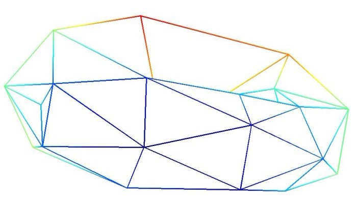
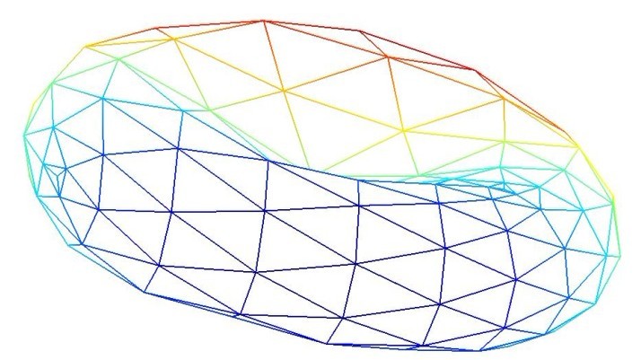
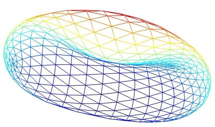
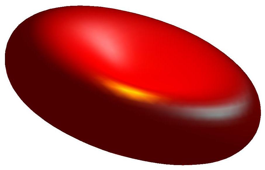
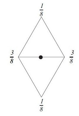
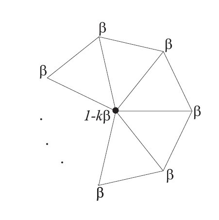
Although the parametric description is more important for us, it is useful to recall the popular algorithmic description of a Loop surface as the limit of an iteration of subdivision steps, see Figure 3; the subdivision step can be succinctly described by the diagrams in Figure 4.
 (a)
(a) 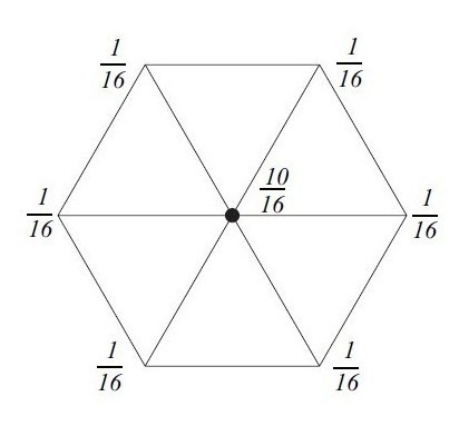 (b)
(b)
 (c)
(c)
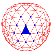
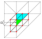
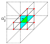
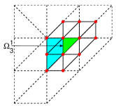
Parametrization of a regular patch. The surface patch associated with a regular face can be parameterized by a linear combination of polynomials with coefficients being the coordinates of the vertices in and their immediate neighbors ordered as in Figure 5(b).444When is close to an extraordinary vertex, it is possible that some of these 12 control vertices coalesce. In such a degenerate situation, one simply repeats the coalescing vertices when using the formula (2.12).(see Figure 5)
| (2.12) |
where , and are the twelve degree 4 polynomials as shown in [69, Page 10-11]. (We do not copy these polynomials from Stam’s paper, but mention that they come from the so-called box-spline.)

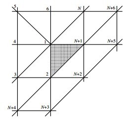
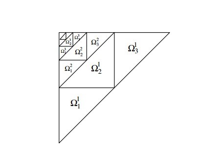 (a)
(b)
(c)
(d)
(e)
For notational convenience, we organize each as a row vector of length , write , and define as a column vector of functions of length 12. Then (2.12) simplifies to
| (2.13) |
Parametrization of an irregular patch. The surface patch associated with an irregular face admits a parametrization which is controlled by control vertices around the face , where is the valence of the extraordinary vertex of . Following Stam’s convention, these vertices are ordered as in Figure 5(d). Like the regular case, is linearly related to the control vertices, so
| (2.14) |
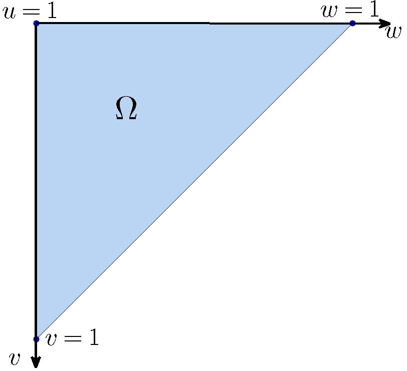
for some basis functions , , implicitly defined by the subdivision process. Unlike the regular () case, none of these basis functions is a single polynomial anymore. Instead, it is an infinite piecewise polynomial, with pieces being the (recursively defined) sub-triangles , , , as shown in Figure 5(e). Note that in this figure the origin corresponds to the extraordinary vertex of .
The parametrization (2.14) is tricky to compute; and this is where Stam’s idea [69, 68] comes in. As in the regular case, write , and . In a nutshell, Stam’s method transforms the control data into ‘eigen- control data’ , so
| (2.15) |
Here is the matrix of (generalized) eigenvectors of the matrix (same notation as in Stam’s paper) that maps the control vertices around to control points in the next subdivision level as shown in Figure 6(b), so where is in a Jordan canonical form. For the Loop scheme, is diagonal when the valence is greater than 3, but has a Jordan block of size 2 when . Since the subdivision process is linear and stationary, i.e. the same linear subdivision rules are used across different scales, recall Figure 3, we have
Putting these together, we have
| (2.16) |
The key point is that these eigenbasis functions are easier to evaluate compared to the original basis functions : When , is diagonal, and we have , apply this recursively we have
| (2.17) |
(Recall Figure 5(e).) As a result, each is specified by three – not infinitely many – polynomials. Also, in virtue of (2.17), and its derivatives can be easily evaluated at arbitrary parameter values after the three polynomials are specified.
These three polynomials can be evaluated based on the same polynomial basis from the regular case (2.12). We write as the (generalized) eigen-vector associated to the eigen-basis function . For , there are suitable linear maps (expressed as in Stam’s paper) so that contains the data at the control vertices that determine the polynomial ; see Figure 6(c)-(e). With an appropriate affine reparametrization of by , denoted as by Stam, this polynomial can be expressed as
| (2.18) |
See [69] for details, e.g. on how to exploit the circulant structure in the matrix in order to facilitate the computation of the related matrices , , .
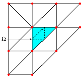
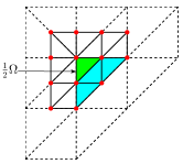
 (a)
(b)
(c)
(d)
(e)
2.2.2 Computation of , , , and their gradients
To summarize the previous section, a regular patch of a Loop subdivision surface is parameterized by a single degree 4 polynomial on the reference triangle for each of the three spatial components, whereas an irregular patch admits a more complicated parametrization over . In either case, an efficient algorithm exists for evaluating the parametrization and its derivatives at arbitrary parameter values . Armed with such evaluation algorithms, we now see how the various functionals and their gradient vectors in (2.1) can be computed.
Formulas for and . We first discuss how to compute the area of a Loop surface and the gradient of with respect to . For each regular face in a control mesh, we write as the area of the surface patch associated to ; and we view as a (real-valued) function of the variables in the array . Similarly, we write as the area of the surface patch associated to an irregular face with an extraordinary vertex of valence ; in this case, we also write . So
| (2.19) |
Recall from (2.13) and (2.15), the parametrization can be written as
| (2.20) |
Note that is linearly related to , whereas the basis functions are independent of . These features allow for an accurate and efficient computation of and , as we shall now see.
We define the map by
| (2.21) |
which picks out the local control data around the face from the global control data .
For convenience, drop the subscript and write instead of . Also, we write , , for the components of and , for their partial derivatives.
Note that
| (2.22) | ||||
Again, we drop the subscript and write , , to refer to the columns of .
When is a regular face, , so
| (2.23) |
The gradient of with respect to , organized as a array (i.e. same dimension as ), can be expressed as:555Here and below, we have to deal with a number of scalar quantities that vary with both the local control data and parameter values (e.g. , , , , , , , , etc..) In order to avoid confusion, we use the notation ‘’ to denote the gradient vector of viewed as a function of ; the gradient ‘vector’ is structured as an array of the same size as . Likewise, the gradient ‘vectors’ , , , are structured as arrays, i.e. the same dimensions as .
| (2.24) |
Similarly,
| (2.25) | ||||
Next, we have
| (2.26) | ||||
Therefore, the local area functional and its gradient
| (2.27) |
can be computed based on the control data and the basis function via (2.23)-(2.26). Together with (2.21) and the chain rule, we can compute the total area and its gradient with respect to by
| (2.28) |
Formulas for , , , and their gradients. Similar to , we aim to express the other three functionals in the C-H model in terms of and the basis functions and . For and , we need an expression for the mean curvature. Recall that
represent the first fundamental form of the surface , whereas
represent the second fundamental form. The mean curvature can be expressed as
| (2.29) |
Therefore
| (2.30) |
where , , . Similarly,
| (2.31) |
Remark 2.4.
When is an irregular face, the mean curvature can potentially blows up when approaching the extraordinary vertex, however it is proved in [61] that the corresponding integrals (called and below) are always finite.
By the divergence theorem, with the choice of the vector field , the volume enclosed by a surface can be expressed as a surface integral:
| (2.32) |
By (2.20), we can express the rightmost integral in (2.30)-(2.32) in terms of and when where ranges over all faces and ranges over all valences existing in the control mesh; we denote the integral by , and , respectively.
We explain how to compute the gradients of , and .
The gradients of , , , , , can be computed as follows
| (2.33) |
By (2.30),
| (2.34) |
Thanks to (2.33), the integrand can be computed by the product and quotient rules. After is computed, can then be computed by
| (2.35) | |||||
Note that every term in the integrand of (2.35) was computed previously.
Finally, for we have
| (2.36) |
With all the local functionals and their gradients with respect to the local control data computed, the global functionals and their gradients with respect to the global control data can be computed exactly as in (2.28):
| (2.37) |
and similarly for , , , .
2.3 Implementation details
In the actual numerical computation of and based on (2.28), we use a symmetric 7-point Gauss quadrature rule on a triangle, with accuracy order 5 (see for example [16]), to approximate the integrals in , , , , and their gradients (recall (2.27), (2.34)-(2.36)). The approximation is done using a composite quadrature on using a uniform grid of size . Typically we use or at coarse subdivision levels, and or at fine levels. We choose to be a dyadic integer in order to take advantage of the subdivision structure of when .
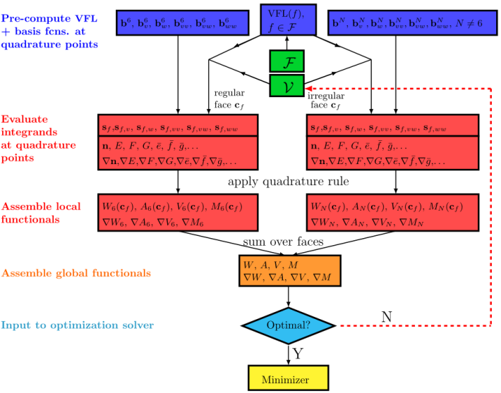
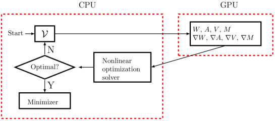
A key implementation detail is that quantities independent of are precomputed before entering the optimization loop. These quantities include and (for only those extraordinary valences that show up in ) and their derivatives at the quadrature points, evaluated using Stam’s algorithm (Sections 2.2.1.) A separate pre-processing step computes the maps for each face in , as depends only on the connectivity information in . Of course, one should not store as a (dense) matrix as suggested by (2.21). Instead, it suffices to store the information in by a list of integer indices in which keeps track of the indices of in the global vertex list ; we denote this list of vertex indices by These preprocessing steps speed up our solver significantly already in a sequential implementation. See Figure 7(left) for the basic organization of our SS solver.
|
|
We note that both the PL and SS functionals are quite easily parallelized; we provide in Wmincon parallel CUDA implementations of all the functionals considered in this article. Together with the aforementioned precomputation trick, we are able to solve a lot of instances of Willmore, Canham and Helfrich problems not addressed in [32]. Figure 7(right) illustrates the basic architecture of our GPU enchanced solver for both the PL and SS methods.
For our implementation of the solver, we primarily use SNOPT [34] and the ‘SQP’ option of fmincon
in the Matlab optimization toolbox.
These solvers are
designed for smooth objectives and constraints,
which is the case for the SS method and most of the PL methods.
An interesting exception is the case of , which is non-smooth
whenever the PL surface has two adjacent triangles of which the four vertices lie on a common circle.
In this case, our use of the non-smooth
optimization algorithm GRANSO [18] was instrumental to the
discovery of Proposition 3.9 below.
3 Analysis
In this section, we give a theoretical justification for why the SS methods succeed in solving the Willmore problem (Section 3.1), but that the PL methods presented in Section 2 are bound to fail (Section 3.2). For computational experiments illustrating the results in this section, see the companion conference paper [12].
3.1 Convergence of SS method
In this section, we establish Theorem 3.8. The argument is based on the existence result for Willmore surfaces established using the direct method in the calculus of variations (Theorem 3.2) [67, 48, 3, 47], and an observation (Proposition 3.1) connecting the existence result to our conforming subdivision methods; the connection requires a density result (Theorem 3.5) from the theory of subdivision surfaces.
A sequence in a space is called a minimizing sequence for a functional if
Proposition 3.1.
Let be a continuous functional on a topological space . Assume that we have a nested sequence of subspaces of such that is dense in . Assume that a minimizer exists. Then any sequence of ‘approximate -minimizers’ , i.e.
is a minimizing sequence for .
Proof: By the denseness assumption, there exists a sequence converging to in . By continuity, . But we also have
so . Thus, is a minimizing sequence for .
Note how this result relies on the conforming and dense nature of the spaces . Notice also that the use of approximate minimizers frees us from the assumption that a minimizer of over each exists.
We now state the key existence result established in [67, 3, 48]. Since we are analyzing a parameteric method, it is more convenient to state the result in terms of parametrizations. For this purpose, we assume is any (reference) genus surface with a smooth enough differentiable structure. A differentiable structure would suffice for our purpose, as it is enough to support the definition of not only and , , but also the whole range of Sobolev spaces , . (See [1] and [31, Section 4.2.3].) We shall work with the Banach space
(normed by ) and the nonlinear, open subspace
| (3.1) | ||||
on which the Willmore energy
is well-defined and continuous.
The following is a reformulation of the well-known existence result pioneered by L. Simon [67] and completed in [3, 48]:
Theorem 3.2 (Existence of -minimizer of genus , via the direct method).
Let be a closed orientable surface of genus with a differential structure. For any minimizing sequence for , there exists a subsequence , and a sequence of Möbius transformations in , such that the sequence of immersed surfaces converges in Hausdorff distance to an immersed surface , . As such, .
Remark 3.3.
The Willmore minimizers are known to be embedded surfaces. We choose to work with general immersed surfaces because in our numerical method we do not have any mechanism built in to avoid self-intersections; another reason is that the solutions of the Helfrich problem for some values of and do have self-intersections.
Remark 3.4.
While [67, 3, 48] prove the existence of a -minimizer over all infinitely smooth genus immersed surfaces, our minimization space is taken to be the bigger (3.1). This causes no problem as is dense in and is continuous. (If is a continuous functional on a topological space , and is a dense subspace of , then any minimizer of must also be a minimizer of .) Here, the definition of , with endowed with a differentiable structure, requires the fact that a maximal -atlas contains a -atlas. In fact there is a real analytic sub-atlas,666The result that every manifold admits compatible and analytic () structures is due to Whitney [73]. with respect to which the minimizer in Theorem 3.2 is real-analytic [67].
The Loop subdivision scheme defines:
-
•
a -compatible atlas, via its characteristic maps, on any base complex , and
-
•
a linear space of scalar-valued subdivision functions at each subdivision level.
The atlas given by the characteristic maps of Loop’s scheme turns into a -manifold. For details, see [1]. The subdivision functions are well-known to be in [60, 80, 79]. By a trivial extension of [1, Theorem 42], we also have
where is given by (3.2) below.
When we extend these subdivision functions componentwise to map into , we denote the corresponding linear space by .
Arden’s thesis [1] essentially establishes the following result. While he focuses on the case, the proof can be extended to a range of values of that is strictly bigger than the interval .
Theorem 3.5.
There exists a such that for any , the space of Loop subdivision functions at all levels is dense in .
Remark 3.6.
The value of above depends on the set of valences present in the underlying simplicial complex, denoted by , and the values of the sub- and sub-sub-dominant eigenvalues, and , of the subdivision matrix corresponding to the different valences . (For the definition of , recall the comments after (2.15) in Section 2.2.1.) We have
| (3.2) | ||||
It is easy to check that approaches 2 from above as . For details, see [76].
In particular, Theorem 3.5 implies, by Morrey’s inequality, that is dense in .
For notational simplicity, we write
Corollary 3.7.
is dense in .777In fact, is dense in for each , so, together with the consequence of Arden’s result, we conclude that is dense in . This stronger result requires extra arguments based on known results in the theory of subdivision surface and an application of Sard’s theorem.
Proof: Since is dense in , and is open in ,
is dense in .
Combining Corollary 3.7 and Proposition 3.1 above, we have the conclusion that if is an approximate -minimizer over in the sense of Proposition 3.1, then the sequence is a minimizing sequence in the setting of Theorem 3.2. So by Theorem 3.2, we have:
Theorem 3.8.
Let be the space of immersed Loop subdivision surfaces on the -times subdivided complex of a genus complex (as above). If is an approximate -minimizer over in the sense of Proposition 3.1, then there is a subsequence so that the surfaces , with suitable Möbius transformations applied, converge in Hausdorff distance to a surface with . This is a genus Willmore minimizer.
This result should explain the empirical success of the SS method; see Section 6 for a possible improvement of this result. In contrast, we next illustrate why the PL -minimizers typically have nothing to do with a continuous Willmore minimizer.
3.2 Failure of Naive PL methods
We begin by establishing a negative result for Bobenko’s Willmore energy, which may sound like an unworthy result given its restrictive consistency property. But here we work in the setting most favorable for in terms of consistency, namely the setting for a regularly triangulated torus. We know from [7] that by successively finer regular sampling and triangulation of a torodial Dupin cylcide at its curvature lines one obtains PL tori with -energy converging to the Willmore energy of the Dupin cylcide. This applies in particular to the Clifford tori (i.e. Duplin cyclides gotten from all possible Möbius transformations of the torus of revolution with radii ration ), which are the only minimizers of the genus 1 Willmore problem [54]. However, we show below that we will never get an approximation of a Clifford torus by minimizing .
The construction used in this proof happens to be applicable, after a twist, to proving a similar negative result for other PL -energies.
3.2.1
For every grid size and , we define a family of triangulated tori, denoted by , , with the following properties:
-
1.
It has vertices, triangles and all vertices have valence 6.
-
2.
All vertices lie on a sphere.
-
3.
The diameter of the ‘tunnel’ of the torus goes to 0 as .
-
4.
The ‘tunnel’ of the torus is triangulated by (long and skinny) triangles.
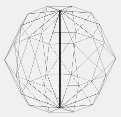
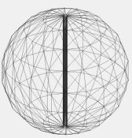
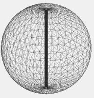
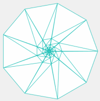
See the first four panels of Figure 8. In details, it is defined as follows. Let , . For , , let
| (3.3) |
Note that maps to . These points on the unit sphere are the vertices of . For the triangulation, each is connected to the six neighbors , , , , , , forming also six triangular faces incident on the vertex. In above, the / in the first and second indices are modulo and modulo , respectively.

 (a)
(b)
(c)
(d)
(e)
(f)
Note that the vertices and , are the vertices closest to the north and south pole, respectively. While these two group of vertices are the furthest apart geometrically, they are connected and form a vertical tunnel of the torus with long skinny triangles.
Denote by the set of all PL surfaces with connectivity of a -regularly triangulated torus and, following [6], for any discrete Willmore energy for PL surfaces, write
Proposition 3.9.
For any grid size , decreases monotonically to as . Hence regardless of , .
Proof: We divide the proof into three steps.
For any triangulated torus defined above,
| (3.4) |
and is an angle formed by the circumscribed circles of the two triangles sharing the edge connecting to [6, Definition 1]. We then notice that
since the six vertices around form a convex neighborhood lying on a common sphere [6, Proposition 1]. By symmetry, and share the same value for all . So we have
It remains to show that decreases monotonicity to as .
To simplify computation, we take advantage of the Möbius invariance of by applying a sphere inversion that maps the unit sphere to the plane. Specifically, we invert about the sphere with radius and centered at the north pole of the unit sphere. This maps the south pole of the unit sphere to the origin, and the north pole to infinity; and it turns our spherical torus to a flattened torus. See Figure 8.
Among the 7 vertices , , , , , , contributing to , , , are close to the north pole, they are sphere inverted to points far away from the origin; , are close to the south pole, they are mapped to points close to the origin. The last two neighbors , are at an approximately constant distance from the north pole: their common polar angle is uniformly larger than, and approaches, as . Therefore, these 7 vertices are mapped to , (in the same cyclic order) with the form
where , as . By scale invariance, depends on through
| (3.5) |
Clearly, (resp. ) increases (resp. decreases) as decreases. So is monotonic increasing for .
Below, we only need the facts that , is monotone in and as .
![[Uncaptioned image]](/html/1901.09990/assets/x18.png) Figure 9: Computation of based on , , ,
, , , .
Among the six circumcircles, two pairs coincide due to the isosceles quadrilaterals
and , thus only 4 circles are seen; they are also
divided into two groups of three (or two rather), displayed in solid and dashed line styles, which are oriented differently when viewed from the outside of the plane.
This is caused by the ‘folding’ of the neighborhood of , and is also why does not vanish despite all the vertices are co-planar.
In this figure, , i.e. ,
and it does not
come from an via (3.5).
Steps and of the proof also do not rely explicitly on (3.5).
Figure 9: Computation of based on , , ,
, , , .
Among the six circumcircles, two pairs coincide due to the isosceles quadrilaterals
and , thus only 4 circles are seen; they are also
divided into two groups of three (or two rather), displayed in solid and dashed line styles, which are oriented differently when viewed from the outside of the plane.
This is caused by the ‘folding’ of the neighborhood of , and is also why does not vanish despite all the vertices are co-planar.
In this figure, , i.e. ,
and it does not
come from an via (3.5).
Steps and of the proof also do not rely explicitly on (3.5).
To calculate we analyze each angle between the circumcircles of the two triangles sharing the edge , now thought of as functions of .
We first notice that the two triangles , sharing are co-cyclic because form an isosceles quadrilateral. Therefore is either or . A closer inspection based on orientation (or simply applying the formula below) tells us that . Similarly, . Next, we show that
| (3.6) |
These limits are not hard to see geometrically based on Figure 9; but to get the finer monotonicity result we resort to algebra and use the formula
where , , , . (Here the and are modulo 6 addition and subtraction operated on the indices .) By computation, we get , , . The limits (3.6) then follow immediately and we have proved that . To see that the convergence is monotone in the original , write
By either a geometric argument or explicitly checking that when , is independent of and . Then again by either a geometric argument or explicitly checking that , is monotone in . Combined with the monotonicity of , the proof is completed.
In the genus case, as long as the connectivity is generic in some sense (see [6, Proposition 9]), the simplicial sphere is inscribable in a sphere and hence has a minimum -energy (0 in Bobenko’s definition of = our definition of ). This is of course the same energy level as what one expects from the smooth setting.
Proposition 3.9 shows that in the genus 1 case, the infimum is never what one expects from the smooth setting, even with the perfectly regular connectivity and regardless of the grid size. Moreover, Proposition 3.9 and computational experiments suggest the following:
Conjecture 3.10.
For any , . Moreover, the infimum is realized by degenerate spheres (, ) and not by any embedded genus 1 PL surface.
This conjecture suggests that a genus 1 -minimizer does not exist, again in contrast to the smooth setting; cf. [67]. It also seems possible to formulate and prove a generalization of Proposition 3.9 to genus , as suggested by the computational result in Figure 10.
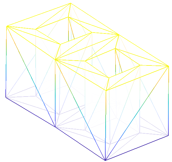
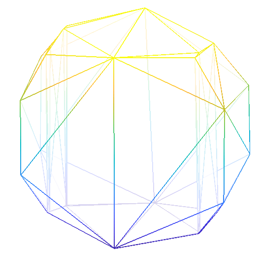
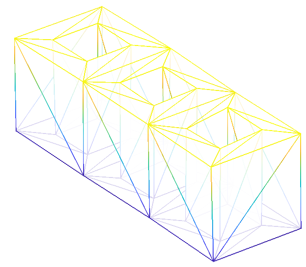
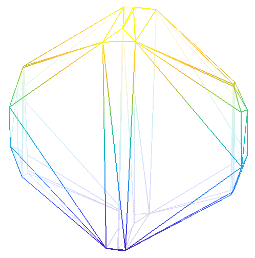 (a)
(b)
(c)
(d)
Back to the genus 1 setting, the proof of Proposition 3.9 suggests the following generalization. Consider the family of planar tori, denoted by
with the same connectivity as before and vertices
We have the following corollary of the proof.
Corollary 3.11.
For any grid size , and fixed ,
and the convergence is monotone.
Proof: All vertices in the intermediate layers () have zero energy. By the calculation in the previous proof, every vertex in the outermost () layer has the same energy , . The fact that this energy is independent of , together with the Möbius invariance of each , actually imply that every vertex in the innermost layer () also has the same energy (independent of ); this can be seen by turning inside out based on inverting about the sphere with radius centered at the origin. Therefore and the result follows by taking .
3.2.2 and
For any mesh with normalized to 1, , we have the following by direct calculation:
| (3.7) | ||||
where . Since the mesh is flat, it does not have an ‘inside’ or ‘outside’, we arbitrarily choose a consistent orientation in order to determine the direction of . (Recall Remark 2.2.)
Next, we show:
Proposition 3.12.
Let the grid sizes be fixed.
-
(i)
For any fixed ,
(3.8) Hence regardless of , .
-
(ii)
For any fixed ,
(3.9) Hence regardless of , .
Proof: All vertices in the intermediate layers () have zero energy. By symmetry, every vertex in the outermost () and innermost () layer has the same energy. So . By scale invariance of , we can assume . By (3.7),
And the proof of (i) is completed.
In contrast to Conjecture 3.10 pertaining to , we observe from computation and preliminary calculations that Proposition 3.12 is not sharp in the sense that the infimum values and are strictly smaller than and , respectively. It is observed that minimizers of both energies are some subtly ‘folded up’ planar meshes.
Although we do not pursue it here, a similar negative result holds for .
The situation for , however, is less well-understood. Note that the outer- and inner-most vertices of satisfy
recall (3.7). This means the corresponding local areas in vanish and . Therefore the planar meshes we considered cannot make small. This is, by design, a key difference between and . However, this does not mean is rid of the type of negative results in Propsoition 3.9 and 3.12. We observe from computations that minimizers of exhibit a similar behavior as those of : they are highly ‘folded up’, but non-planar, meshes, with energies less than ; see Figure 11(a)-(b).
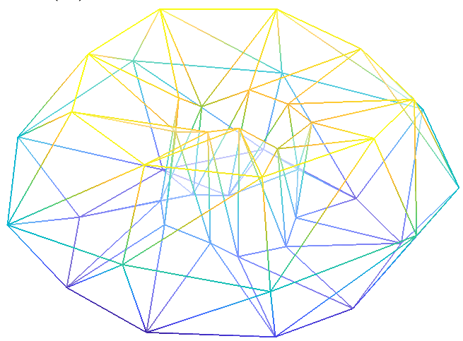
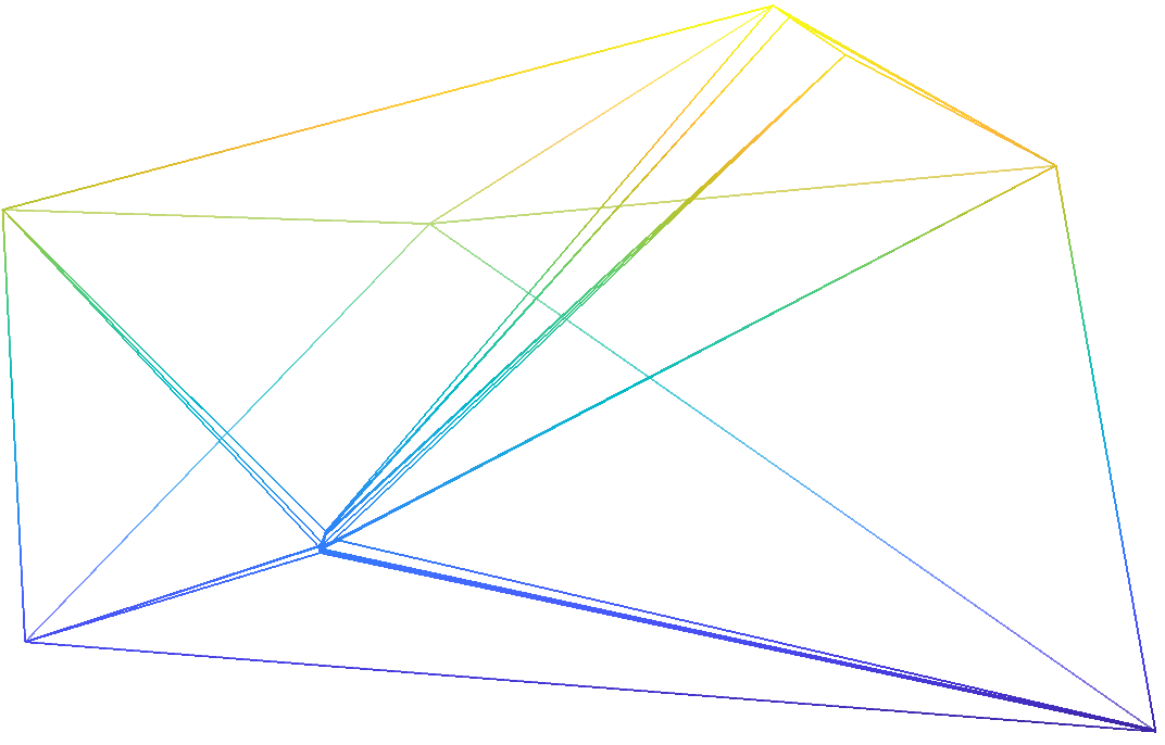
 (a)
(b)
(c)
(d)
3.2.3 Genus 0 case
In the genus 0 case, computational experiments suggest that , and fail in a way similar to the genus 1 case; we believe that a genus 0 version of Proposition 3.12 can be established.
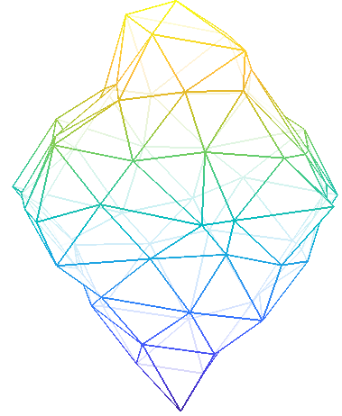
However, the situation for and are different. Recall that the Willmore energy of any closed surface should always be greater than or equal to , with equality attained only by the round sphere [74]. is designed to satisfy this ‘ground-state’ property: , with equality holds when and only when the PL surface is a convex polyhedron inscribed in a sphere [6, Theorem 5]. So there cannot be a genus 0 version of the negative result in Proposition 3.9. An empirical finding is that actually works well for the genus 0 Willmore problem. See Figure 11(c)-(d), which shows one of the many trials of the experiment with a randomized initial mesh; all trials of -minimization applied to a genus 0 mesh result in a near round sphere with slightly larger than .
4 A Regularized PL Method
All failures we observed have one thing in common: triangles with bad aspect ratios develop. This is of course a familiar issue in FEM and mesh generation, but in the moving surface context here the issue seems different and understudied. In previous work by Hsu-Kusner-Sullivan [40], procedures such as ‘vertex averaging’, ‘edge notching’ and ‘equiangulation’, implemented in the Surface Evolver [10, 11], are used to fix up triangles with bad aspect ratios along the way of the optimization process. While such ‘mesh smoothing’ procedures are probably well studied in the mesh generation community, when applied to the geometric variational problems here the approach seems ad-hoc and difficult to analyze mathematically.
Our numerical methods, based on either PL or SS, are parametric in nature. Yet, the variational problems are geometric and their solutions are independent of parametrization. This creates another problem instead of solving the existing one! Our observation is that it is possible to design a method in such a way that the two problems cancel each other.
Since the solution is independent of parametrization, we may request the parametrization to be (approximately) conformal,888Not to be confused with the conformality in finite-element methods. i.e. angle preserving, with respect to an appropriate conformal structure in the reference manifold . If such a property can be built into a -minimizing process, the method would only search over PL surfaces without long skinny triangles.
The approach adopted here is inspired by the classical uniformization theorem and results in harmonic maps [29, 27, 28], as well as the relatively recent developments in computational conformal geometry, see [35, 17, 36, 24, 53, 38, 37] and the references therein.
In a finite-dimensional approximation of the solution surface, we cannot expect to have exactly conformal parametrization. To fix the idea, let us first consider the problem of finding a conformally parameterized Willmore surface in the smooth setting.
4.1 Ideas in the smooth setting
We use the theory of harmonic maps. From now on we assume is a Riemann surface. For any map , we can define its Dirichlet energy by
| (4.1) |
where is the Hilbert-Schmidt norm first defined based on some Riemannian metric on and the standard Riemannian metric in , followed by the observation that is invariant under any conformal change of Riemannian metric in the domain; see [29, Pg. 126]. This invariance is specific to , and it means that the Dirichlet energy depends only on the conformal structure of . Next, we have the following well-known result:
Theorem 4.1 ([29]).
For any immersion , . Equality holds when and only when is conformal.
It is already evident from the theorem that the difference measures the deviation of being conformal. In fact, the difference can be explicitly expressed by a conformal energy expressing the deviation of from satisfying the Cauchy-Riemann equations.
Proposition 4.2.
Let be a Riemann surface and for a fixed . Assume that:
-
(i)
a minimizer exists for all small enough ,
-
(ii)
exists. (Here convergence is in the topology of .)
Then
-
(I)
is a Willmore minimizer, i.e. it is a solution of the Willmore problem . Moreover, any other Willmore minimizer satisfies .
-
(II)
If the conformal structure on is such that there exists a conformal parametrization of the surface , then , and in fact for any , is a conformal parametrization of a Willmore minimizer, i.e. and for any .
Proof: We first argue that must be a Willmore minimizer. If not, there exists an such that . But then for small enough , we must have . (If , this holds for any , otherwise choose .) By (ii) and the continuity of and , we have
This contradicts assumption (i), and we have proved the first claim in (I). We now argue the second claim again by contradiction. Let be any other Willmore minimizer, so . Assume the contrary that . Then for any . Again by (ii) and the continuity of and ,
This contradicts (i), so . By Theorem 4.1, we also have .
By Theorem 4.1 and the assumption of the conformal structure on , the minimum values of and over , namely and , are attained simultaneously by some . But any , being a minimizer of , must also be such a joint minimizer. Then, by continuity, is such a joint minimizer as well.
Remark 4.3.
In the most ubiquitous spherical topology, there is only one conformal structure up to conformal equivalence. Together with the genus 0 case of the uniformization theorem, the assumption in (II) above is satisfied automatically when is the Riemann sphere. In this case, solving the -penalized Willmore problem with any penalization parameter – not necessarily small – would deliver a conformally parameterized Willmore surface. In the higher genus cases, there is a 1 (when ) and (when ) complex-dimensional space of conformal structures [42], and typically we do not know a priori the ideal conformal structure for the Willmore surface. With the correct conformal structure, a conformally parametrized solution is impossible, but Proposition 4.2 says (in (I)) that the solution of the -penalized Willmore problem with a small penalization parameter would still deliver a Willmore surface parameterized as conformally as possible in the non-ideal conformal structure.
We shall use this result to guide us to develop an algorithm for fixing the naive PL method. Before we proceed, we present a version of Theorem 4.1 for PL surfaces.
4.2 A PL version of Theorem 4.1
Theorem 4.5 below is well-known to experts in computational conformal geometry; see, for example, [17, 35] and references therein. We provide a proof for it not only for the sake of self-containedness but also to help us to understand its subtle relationship with the smooth counterpart Theorem 4.1.
Definition 4.4.
Let be a simplicial surface.
-
1.
A angle assignment on is an assignment of angles to every triangle in .
-
2.
A PL immersion is called angle preserving if every triangle in is similar to , i.e. they share the same angles.
The notion of angle assignment in 1. above actually defines a conformal (or complex analytic) atlas in the traditional sense via a construction by L. Bers. The construction essentially exploits the fact that the map
maps the interior – but not the boundary – of a cone in with apex angle bihorlomorphically to the interior of a cone with apex angle (assume ). For details, see [24, Section 2] or [5, Lecture 2]. In these references, the conformal structure is supposed to be induced by a PL embedding . However, it is obvious that the conformal atlas defined there depends only on the angle assignment induced by the embedding. We note that, however, many different angle assignments may give rise to equivalent conformal structures on . For example, in the genus 0 case, any two conformal structures are conformally equivalent.
Once such a conformal structure is defined, and noting also that piecewise linear maps have square integrable derivatives, the Dirichlet energy of a PL immersion is well-defined according to (4.1). Of course, the area is also well-defined in the standard sense. As such, the first half of Theorem 4.1, which requires only to be in , holds verbatim, i.e. . However, the second half of Theorem 4.1 is less obvious, as the standard definition of conformality for smooth maps does not seem to apply directly to PL maps. Fortunately, if one simply defines conformality for PL immersions as in Definition 4.4, we get the following result:
Theorem 4.5 (PL version of Theorem 4.1).
Let be a simplicial surface with an angle assignment. For any PL immersion , . Equality holds when and only when is angle preserving.
Proof: Bers’ conformal structure and the fact that depends solely on the conformal structure guarantee that in the interior of every triangle of , the Dirichlet energy (4.1) can be computed as
| (4.2) |
where “” is the area element in the coordinates of after we identify with a triangle on the plane with the angles assigned to . For details, consult [24, Section 2]. For any , is a linear map and we may represent it by a rank 2 matrix , so
| (4.3) |
Since
where and , both positive, are the eigenvalues of , . Moreover, equality holds above if and only if for all triangles , which is exactly the case when is angle preserving.
In the PL setting above, the Dirichlet energy can also be expressed by the cotangent formula
| (4.4) |
where is the edge of opposite the angle , and and are the angles opposite the edge in the two incident triangles. This follows immediately from a simple formula: if is a linear function on a triangle , then
where are the vertices of and is the angle at vertex .
Remark 4.6.
A subtle point here is that if we simply define the Dirichlet energy of a PL immersion by either (4.3) or (4.4), then both the formulation and the proof of Theorem 4.5 completely bypass Bers’ construction. We may then view the ‘Bers-free version’ of Theorem 4.5 as a discrete analog of Theorem 4.1. This would be in line with the spirit of ‘discrete differential geometry’ [8]. We find it instructive to know that Theorem 4.5 and Theorem 4.1 are not only analogous, but that one may view (at least the first part of) the former theorem as a special case of the latter classical result.
Finally, we note that when the angles assigned to are exactly those of the triangles in , then it is a tautology to say that is angle preserving. In this case, is given by the cotangent formula (4.4). This, in turn, can be used to give an alternative proof for the cotangent formula of in (2.4), explaining also why the two seemingly unrelated cotangent formulas look so alike.
4.3 A penalized PL method
Inspired by Proposition 4.2, we propose a numerical solution to the Willmore, Canham or Helfrich problem based on solving:
| (4.5) |
Here represents any of the PL Willmore energy discussed earlier, and is the Dirichlet energy of the piecewise linear immersion (determined by ) of the domain simplicial complex (determined by the face list ) endowed with a suitable angle assignment.
Proposition 4.2 suggests that, while it is not necessary, it would be best if we use a conformal structure for which a conformal parametrization is possible, as it would free us from the need of making the penalization arbitrarily small, thus giving us a more efficient numerical method. In the genus 0 case, there is only one conformal structure up to conformal equivalence. So we may simply assume every triangle in to be equilateral. Under this angle assignment, the Dirichlet energy is, by (4.4),
| (4.6) |
As mentioned, we can still use (4.6) in the higher genus cases, as long as we use a small enough ; see the genus 1 results in the next section.
4.4 Computational results
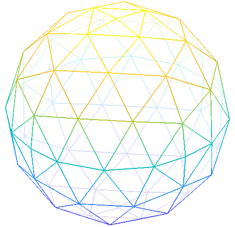
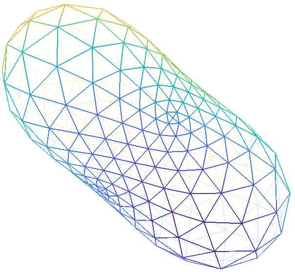
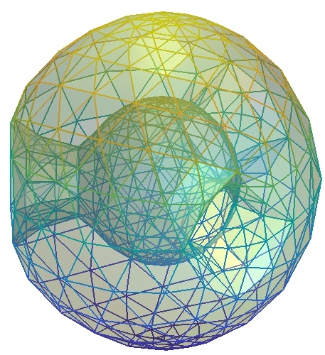
Figure 12 shows how the -penalized method (4.5) performs on the genus 0 Canham problem with reduced volume/isoperimetric ratio in three different intervals known to give the shapes of a stomatocyte, discocyte (red-blood cell) and prolate. The results are consistent with those reported in the biophysics literature, and those produced by SS methods. See Section 5 for a more thorough comparison of different methods applied to these problems.
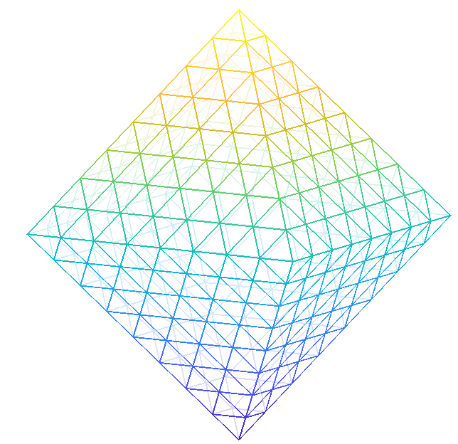
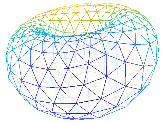
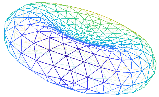
 (a) initial mesh
(b) , stomatocyte
(c) , oblate
(d) , prolate
In each case, we found that the numerical solution changes little with the choice of , which is consistent to the conclusion of Proposition 4.2. Also from the fact that is pretty close to the area , we conclude from Theorem 4.5 that the PL embeddings are close to being angle preserving.
In the higher genus case not all conformal structures are conformally equivalent. In the genus 1 case, the uniformization theorem implies that our solution surface can be mapped conformally to a flat torus. However, there is a one-complex dimensional family of non-equivalent conformal structures on a flat torus.
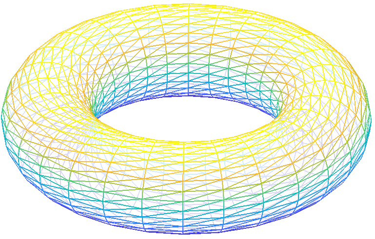
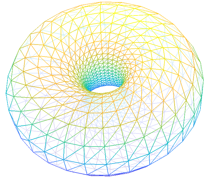
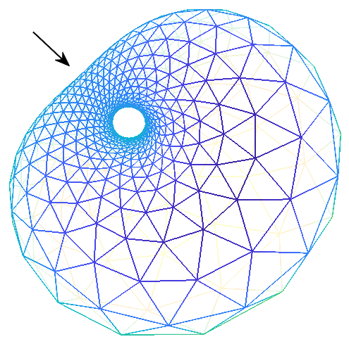
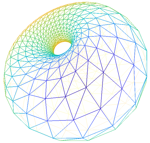
Here, we use to solve the genus 1 Willmore problem problem. And we choose the domain Riemann surface to be a regularly triangulated parallelogram with sides and on the complex plane. We denote by – easily computable according to (4.4) – the corresponding Dirichlet energy. In this case we know that the solution is the Clifford torus, with Willmore energy , and the ideal conformal structure is that of a square, i.e. . We compare the result with what we get by using the conformal structure, i.e. . See the results in Figure 13 (b) & (c). We see that by using the ideal conformal structure the PL Willmore energy is closer to the expected , and is closer to zero. (With the incorrect conformal structure, we cannot expect to have a conformal parametrization, and hence we cannot expect as the grid sizes grow.) Also with the incorrect conformal structure the axis-symmetry is broken, the surface looks like a Möbius transformation of the surface of revolution Clifford torus (a Dupin cyclide), but with an indentation, indicated by the arrow in Figure 13 (c). The indentation suggests that the method is not capturing the shape accurately. However, by reducing from to , the indentation disappears and the resulted surface becomes a more accurate approximation to a Clifford torus. This is completely in line with what Proposition 4.2 says.
In Figure 13(d), we show a numerical solution of the genus 1 Canham problem with reduced volume , it is believed that the solution is a unique Möbius transformation of the surface of revolution Clifford torus; see [77]. And we also know that the ideal conformal structure to use is the square one. The solution is accurate even with a relatively big penalization factor. Again, it is in agreement with Proposition 4.2.
 (a) initial mesh,
(b)
(c)
(d)
triangles
,
,
,
5 Further Computational Results and Symmetry Preservation
A group of biophysicists obtained a plethora of computational results for the Canham and Helfrich problems for low genus and various constraint parameters [56, 57, 51, 43, 75, 41]. Many interesting observations are made about the uniqueness, non-uniqueness, symmetry and phase transition properties for these problems. So far few of these observations have been justified mathematically. In fact, the mere existence of a solution of the Canham problem, i.e. existence of a Willmore minimizer with a prescribed isoperimetric ratio and genus, is an unsolved problem in geometric analysis when the genus is larger than 0 [46]; for the genus 0 case, see [65]. The existence of solution of the Helfrich problem has not been addressed so far. Moreover, in the biophysics literature, the numerical behavior of the optimization method is never addressed; the only information we have is that Brakke’s Surface Evolver was used, as in the experiments done in [40].
In this final technical section, we give a few comparisons of the different implementations of the PL and SS methods presented earlier. We must begin with a confession:
The algorithms developed in Section 2 and 4 only address how to discretize the variational problem into a standard finite-dimensional constrained optimization problem of the form
and the theory in Section 3 sheds some light on what it means to the variational problem if
we manage to solve the optimization problem. Needless to say, solving the latter problem itself
— a high-dimensional, nonlinear, nonconvex, constrained optimization problem — is a major
challenge and there are many algorithms and solvers available. In our experiments,
we use the following three solvers:
(i) fmincon in the Matlab optimization toolbox, (ii) SNOPT [34] and
(iii) GRANSO [18].
Given the complexity of these solvers, there are countless issues to explore and compare in conjunction with our problems. We shall focus mainly on the approximation and symmetry properties of the optimization problems arising from the PL and SS methods, and will briefly touch upon the existence issue of these optimization problems. With regrets, we will not address the important question of the efficiency of solving these problems by various optimization alogirithms/solvers.
5.1 Comparison I: PL vs SS
The original expectation is that a PL method is less accurate than the higher order SS counterparts, only that we found in Section 3.2 and 4 that the non-conforming nature of PL methods require us to introduce regularization. We are finally in a position to compare the accuracy of our PL and SS methods.
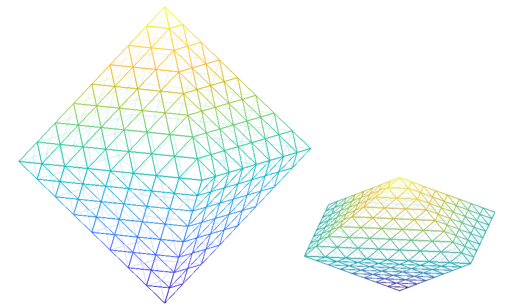
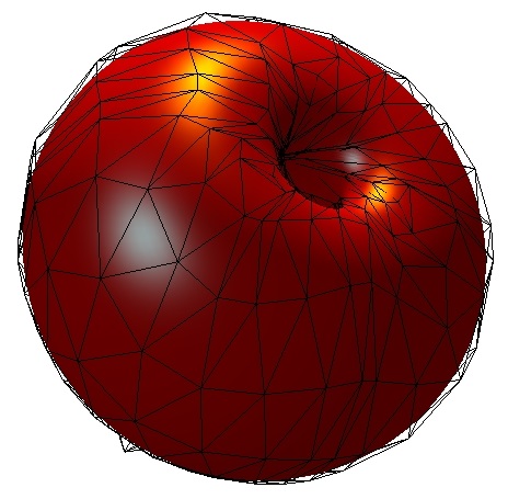
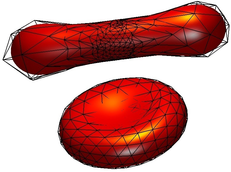
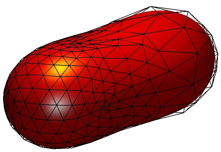
It is known from Schygulla [65] that -minimizer of genus 0 with any prescribed isoperimetric ratio exists, and that the minimum Willmore energy is strictly less than . In Figure 12, we solve for these minimizers using a regularized PL method for , and . The case is arguably the most difficult one as an ‘invagination’ develops in the vesicle; in this case the PL Willmore energy computed is bigger than , see the caption of Figure 12(b). We now solve the same three problems but using our Loop SS method.
 (a) initial meshes
(b)
(c)
(d)
(top),
(bottom)
Without an explicit representation of the solution, we cannot directly compare the accuracy of the PL and SS methods. However, we see from our computation that in each case, the (true) Willmore energy of the SS approximation is lower than the (PL) Willmore energy of the PL approximation. In the case, the Willmore energy of the SS approximation is less than , as it should according to Schygulla’s result. These observations are consistent with the higher accuracy order of SS compared to PL approximations.
5.2 Comparison II: Symmetry preservation vs symmetry breaking
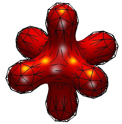
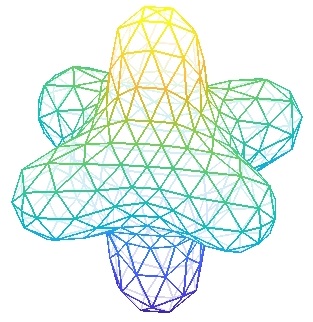
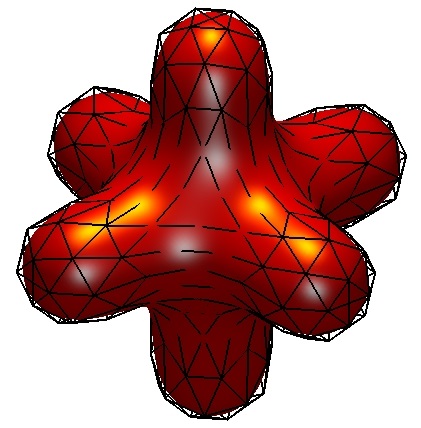
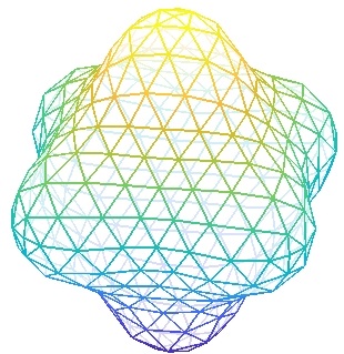
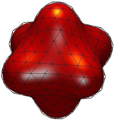
The results in Figure 12 and 14 are based on the fmincon and SNOPT solvers.
With our third solver, GRANSO, and the same octahedral initial mesh in Figure 12(a),
we got totally different, non-global local minimizers which inherit the octahedral symmetry from the initial mesh;
see Figure 15.

 (a)
(b)
(c)
(d)
(e)
(f)
Apparently, the underlying constrained optimization algorithm employed in the GRANO solver has a symmetry preserving
property. To the best of the authors’ knowledge, this kind of
symmetry preservation and breaking
properties is not well-addressed in the optimization literature. Here, we
observe a fundamental difference among the three solvers: GRANSO is capable of preserving
symmetry in the sense below,999The authors of GRANSO designed the solver with the intention that it can handle non-smooth problems, but without the intention for symmetry preservation.
Our original use of it is due to the non-smoothness of ; recall Section 3.2.
The problems in this section are smooth and we are only exploiting its symmetry preserving property.
while fmincon and SNOPT are capable of breaking symmetry.
Symmetry preservation of gradient and Newton descent. To define ‘symmetry preservation’ precisely, we begin with the following fact about gradient flow which is well-known to geometers: Let be a Riemannian manifold, and be a group of isometries acting on . If we have a smooth -invariant functional , i.e. for all and , then the gradient flow map is also -invariant: . In particular, if is a symmetric point (i.e. for all ), then so is for any .
Here we prove a version of this fact tailored for our setting; the proof easily extends to methods beyond gradient descent.
Any one of our geometric functionals , , or is a -invariant functional, i.e.
| (5.1) |
There is yet another invariance, namely invariance under simplicial isomorphisms. For a face list in a triangle mesh that specifies the simplicial complex structure of the mesh, there is a subgroup, denoted by , of the permutation group of that corresponds to the group of simplicial isomorphisms. In other words, re-labelling the vertex indices according to the permutations in gives the same triangulation (i.e. the geometric realization of the simplicial complex.) Our geometric functionals must satisfy
| (5.2) |
Definition 5.1.
Let be a finite subgroup of .101010The Schoenflies notation can be used to refer to any one of the possibilities of such a . A simplicial complex, specified by a face list of a mesh, is said to support (the symmetry group) if is isomorphic to some subgroup of . In this case, we denote the correspondence by
A mesh in is called -symmetric if for every , . Equivalently, if we define the group action of on the manifold by
then (with fixed) is -symmetric if and only for all .
In this setting, the set of symmetric points is a linear submanifold of . Note that whenever the underlying simplicial complex supports the symmetry group , then by (5.1) and (5.2) is -invariant in the sense that
| (5.3) |
A gradient flow of satisfies and the corresponding gradient descent algorithm satisfies
By the chain rule applied to (5.3), . Then, by orthogonality, . We can see that a gradient descent, which we formally denote by , satisfies the transformation property:
In particular, gradient descent preserves the symmetry of the previous iterate. It is also easy to check that the quasi-Newton BFGS method is symmetry preserving.
In our application, can be chosen to be the penalty function of a Helfrich problem:
Since inherits the -invariance from its constituent objective and constraint functions, any one of the gradient descent, Newton or BGFS methods applied to would furnish a symmetry preserving algorithm for approximately solving the constrained optimization problem. Note that the symmetry preservation property holds regardless of the penalization parameter or the line search parameters , which vary from iteration to iteration. However, the penalization parameter has be big enough in order for the constraints to be approximately satisfied.
Sophisticated BFGS-SQP based
solvers such as SNOPT, GRANSO and fmincon are not simply based on applying the BFGS method
to the penalty function,
and those who engineer these solvers do not have the symmetry preserving property
in mind.
It is therefore interesting to see from the experiments that the BFGS-SQP method used in GRANSO preserves symmetry almost perfectly, even in the presence
of roundoff errors.
We shall present a formal justification of this observation in a separate report.
In principle, we can optimize in a symmetry preserving way by optimizing only over the degrees of freedom that determine the control mesh up to the desired symmetry, as is done in Brakke’s Surface Evolver or [78]. This has the added advantage of reducing the dimensionality of the problem, but requires an extra effort in coding and algorithmic development. GRANSO, or any solver with the same symmetry preserving property, frees us from the latter.
5.3 Comparison III: Symmetric vs ‘Best’ Minimizers
The example in the previous section says the obvious: applying a symmetry preserving optimization algorithm to an initial guess with the wrong symmetry is not going to solve the problem. What if we have the correct symmetry? Our next experiment, based on comparing different solvers, shall reveal a rather subtle feature not of the optimization algorithms, but of the optimization problems themselves.
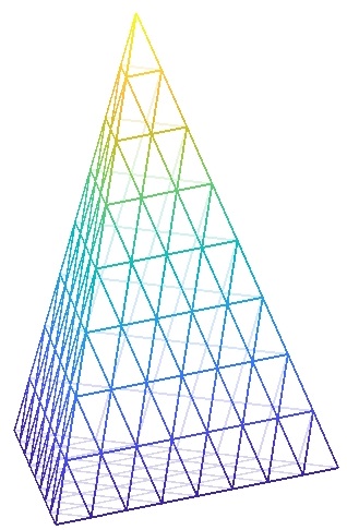
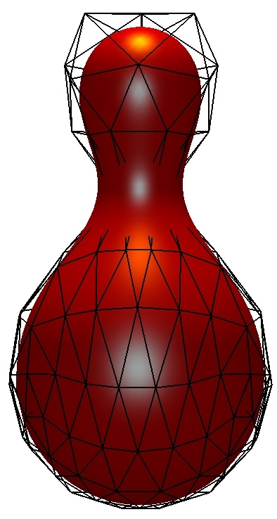
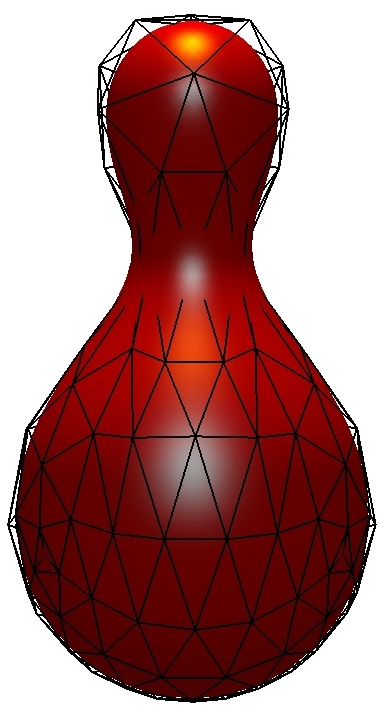
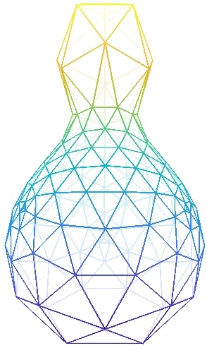
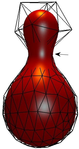
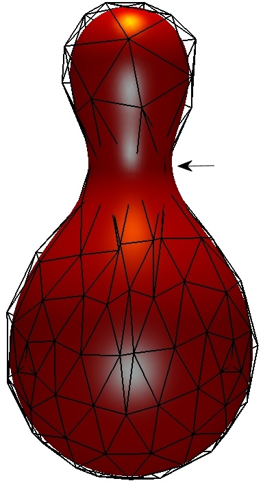
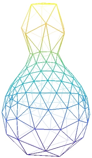
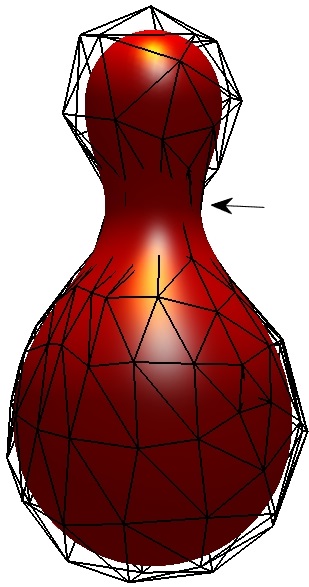
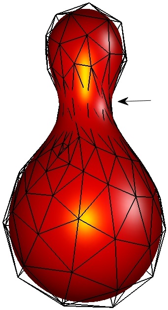
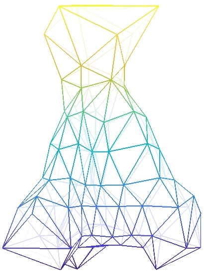
We consider the genus 0 Helfrich problem with . It is believed that the minimizer is a surface of revolution with a pear shape. The two initial meshes in Figure 14(a) have extra symmetries (octahedral and symmetry) not possessed by a general surface of revolution. Applying the GRANSO solver, which presumably preserves symmetry, would fail to yield the correct solution; it is indeed what we observe from computation. If we use instead GRANSO with a -symmetric initial mesh with no extra symmetry, we expect to approach the correct minimizer with a -symmetric approximation, and it is again what we observe from computation; see Figure 16(i). In the case of the C2g0 and Loop SS methods, SNOPT and fmincon break the symmetry, as shown in Figure 16(ii) and (iii). If one zooms into the control meshes, one sees that the symmetry is clearly broken around the neck area (indicated by the arrows in the relevant panels). Note that the neck area is also where the absolute Gauss curvature of the pear surface is the highest.
 initial mesh
C2g0
Loop
PL
 20.432
20.48
21.89
C2g0
Loop
PL
 20.427
20.47
21.87
C2g0
Loop
PL
 20.426
20.44
infeasible
(i) GRANSO
(ii) SNOPT
(iii) fmincon
The asymmetric approximations to the (presumably symmetric) solution, produced by SNOPT and fmincon, have slightly smaller Willmore energies than those of the symmetric approximations produced by GRANSO. We believe that this is not caused by roundoff errors or truncation errors from numerical integration.
In (i), GRANSO terminates gracefully with a stationarity condition satisfied up to a tolerance. This suggests that GRANSO produces a -symmetric critical point of the problem that is a local minimizer of the Helfrich problem with the added -symmetry constraint. By the principle of symmetric criticality [59], this critical point must also be a critical point of the full Helfrich problem (without any symmetry constraint.) Since (ii) and (iii) strongly indicate that this critical point is neither a local nor global minimizer, we are led to believe that it is a saddle point of the Helfrich problem.
5.4 -minimizers of genus and Lawson’s surfaces
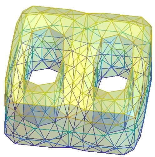
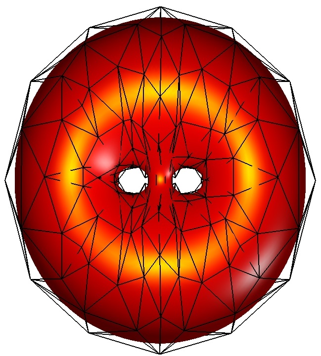
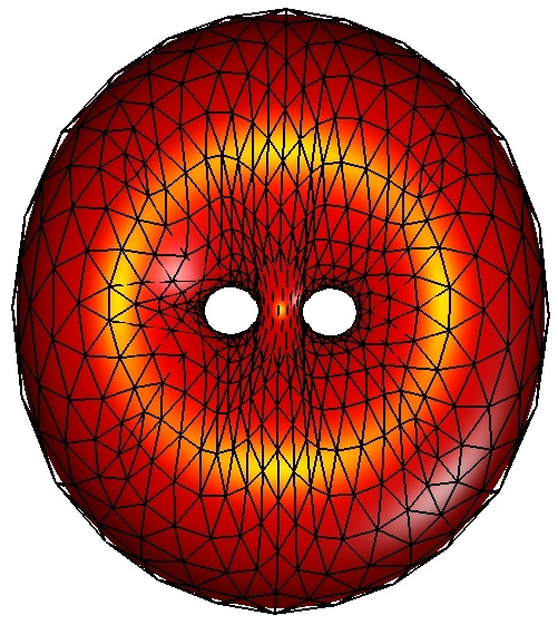
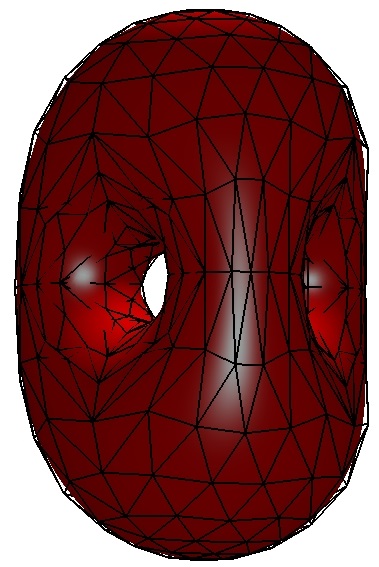
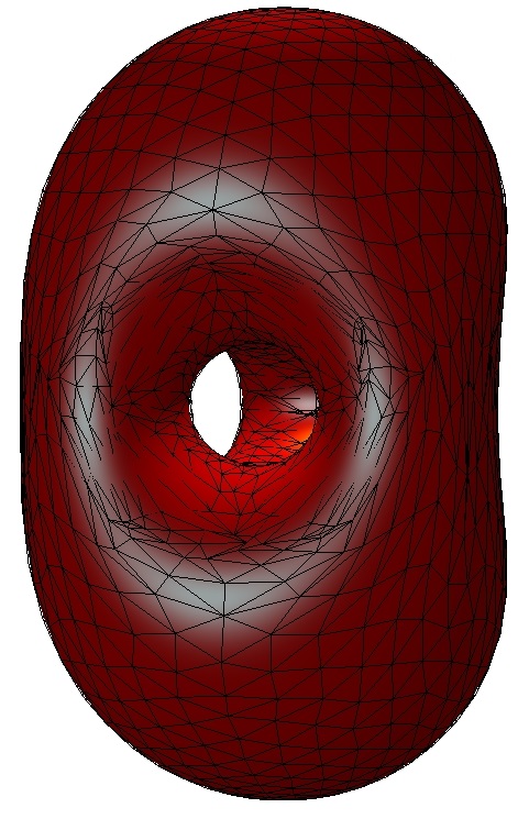
It is conjectured that the stereographic images of Lawson’s minimial surface in [49] are the only -minimizer of genus in . The term ‘Willmore conjecture’ – now the celebrated Marques-Neves theorem [54] – refers to the case of this more general conjecture. Here, we use our SS method to illustrate this conjecture for . There are two stereographic projections of from to that give the resulting surfaces a or symmetry. We create initial control meshes with these two symmetries and solve the Willmore problem using our Loop SS method and the symmetry-preserving GRANSO solver. We also apply an iterative refinement, exploiting the underlying subdivision structure, to improve the accuracy of the solutions. The resulting surfaces are visually the same as the corresponding stereographic projections of Lawson’s , and have the same Willmore energy of approximately 21.9. (The two surfaces are meant to be Möbius transformations of each other.) See Figure 17.
 (a) initial mesh
(b)
(c)
(d) initial mesh
(e)
(f)
vertices
d.o.f.
d.o.f.
vertices
d.o.f.
d.o.f.
The same code for generating Figure 17, available in the Wmincon package, works for any genus . We have used it to empirically verify the generalized Willmore conjecture for up to genus .
6 Conclusion and Future Work
Admittedly, our analyses in Section 3 only address one fundamental aspect of what we may expect from the PL and SS methods. Even so, both the positive and negative results there have much room for improvements.
The positive result Theorem 3.8 asserts that some subsequence of a sequence of discrete minimizers converges to a minimizer of the continuous problem; the result does not say anything about the rest of the sequence. Does it mean that some elements of our hard-earned sequence may have nothing whatsoever to do with any minimizer of the continuous Willmore problem, even for arbitrarily large ? We do not believe so, as we may use Theorem 3.8 repeatedly in the following way:
-
•
Apply the theorem to extract a convergent subsequence (convergent in the sense stated in the theorem) from
-
•
Remove this subsequence from the original sequence, the remaining sequence is still a minimizing subsequence.
-
•
Apply the theorem again to extract a convergent subsequence from the remaining sequence.
-
•
…
Loosely speaking, this process should exhaust the whole sequence, and hence it seems plausible we can partition the original sequence into subsequences each of which converges to some Willmore minimizer. We therefore expect the following to hold true:
Conjecture 6.1.
Let be any minimizing sequence in the setting of Theorem 3.2. (In particular, can be an approximate -minimizer over , as in Theorem 3.8.)
-
(I)
There is a sequence of Möbius transformations in such that the sequence of surfaces can be partitioned into subsequences each of which converges in Hausdorff distance to some Möbius representative of a genus Willmore minimizer.
-
(II)
If we further assume that the Willmore minimizer of genus is unique up to Möbius transformations, as would be implied by the generalized Willmore conjecture (see Section 5.4), then the whole sequence of surfaces in (I) converges in Hausdorff distance to some Möbius representative of a genus Willmore minimizer.
The situation for the Canham and Helfrich problems is more challenging. On the geometric analysis side, even the existence problem for the Canham problem is not resolved for every positive genus and all isoperimetric ratios; see [65] and [46]. (In the genus zero case, Schygulla [65] solves the existence problem for all isoperimetric ratios.) On the numerical analysis side, a key difficulty is to prove the corresponding density result Corollary 3.7 with a fixed isoperimetric ratio constraint, i.e.
Conjecture 6.2.
For any is dense in , where is the space of all immersed Loop subdivision surfaces over a closed oriented with isoperimetric ratio and is the space of elements in with isoperimetric ratio .
If this difficulty can be overcome, we expect that a result similar to Theorem 3.8 can be obtained for the Canham problem based on the existence results for the Canham problem established in [65] and [46]. The Helfrich problem is out of reach for now.
The negative results Proposition 3.9 and 3.12 are established on a case by case basis. Perhaps there is a universal negative result asserting that any consistent PL Willmore energy would fail in a similar manner. Besides the very special genus 0 cases for and (recall Figure 11), it appears that the space of PL surfaces (of a fixed combinatorial type) is ‘too big’ that minimizing any PL -energy over it would always take us to some PL surface inconsistent with any smooth surface. It is an open question to formulate and prove this speculation.
A deeper mathematical study of these issues and the proposed regularization in Section 4 may lead to understandings of other non-conforming methods, such as the ones proposed in [9, 63]. However, as mentioned in the introduction, the methods in [9, 63] are in the spirit of ‘discretizing a minimization,’ whereas the methods studied in this article are in the spirit of ‘minimizing a discretization.’ It is an open question to see if these different methods can be analyzed in a coherent way.
It will be interesting to address rate of convergence issues in the future. Arden’s result [1, Theorem 2] establishes a rate of convergence of Loop subdivision functions in , but we believe that the rates established there are suboptimal. Also, the approximation rates of other schemes (e.g. [15]) are yet to be explored. Regardless, further techniques are needed for transferring any approximation rate result in the pure approximation setting to an approximation rate result for the geometric variational problems. To this end, we expect knowledge on the second variation of the Willmore energy, such as the results by Weiner [72], will be helpful.
References
- [1] G. Arden. Approximation properties of subdivision surfaces. PhD thesis, University of Washington, Department of Mathematics, 2001. Available at https://sites.math.washington.edu/~duchamp/preprints/arden-thesis.pdf.
- [2] J. W. Barrett, H. Garcke, and R. Nürnberg. Finite element approximation for the dynamics of asymmetric fluidic biomembranes. Math. Comp., 86(305):1037–1069, 2017.
- [3] M. Bauer and E. Kuwert. Existence of minimizing Willmore surfaces of prescribed genus. International Mathematics Research Notices, 2003(10):553–576, 2003.
- [4] T. Baumgart, S. T. Hess, and W. W. Webb. Imaging coexisting fluid domains in biomembrane models coupling curvature and line tension. Nature, 425:821–824, Oct 2003.
- [5] L. Bers. Riemann Surfaces. Courant Institute of Mathematical Sciences, New York University, New York, 1958.
- [6] A. I. Bobenko. A conformal energy for simplicial surfaces. In Combinatorial and computational geometry, volume 52 of Math. Sci. Res. Inst. Publ., pages 135–145. Cambridge Univ. Press, Cambridge, 2005.
- [7] A. I. Bobenko and P. Schröder. Discrete Willmore flow. In In Eurographics Symposium on Geometry Processing, pages 101–110, 2005.
- [8] A. I. Bobenko and Y. B. Suris. Discrete differential geometry, volume 98 of Graduate Studies in Mathematics. American Mathematical Society, Providence, RI, 2008.
- [9] A. Bonito, R. H. Nochetto, and M. S. Pauletti. Parametric FEM for geometric biomembranes. J. Comput. Phys., 229(9):3171–3188, 2010.
- [10] K. A. Brakke. The Surface Evolver. Experimental Mathematics, 1(2):141–165, 1992.
- [11] K. A. Brakke. Surface Evolver manual version 2.70. Available at http://facstaff.susqu.edu/brakke/evolver/downloads/manual270.pdf (2018/04/20), August 2013.
- [12] J. P. Brogan, Y. Yang, and T. P.-Y. Yu. Numerical methods for biomembranes based on piecewise linear surfaces. In F. A. Radu, K. Kumar, I. Berre, J. M. Nordbotten, and I. S. Pop, editors, Numerical Mathematics and Advanced Applications: ENUMATH 2017, volume 126 of Lecture Notes in Computational Science and Engineering. Springer Nature Switzerland AG, 2018.
- [13] A. M. Bruckstein and A. N. Netravali T. J. Richardson. Epi-convergence of discrete elastica. Applicable Analysis, 79:137–171, 2001.
- [14] P. B. Canham. The minimum energy of bending as a possible explanation of the biconcave shape of the human red blood cell. Journal of Theoretical Biology, 26(1):61–76, 1970.
- [15] J. Chen, S. Grundel, and T. P.-Y. Yu. A flexible subdivision scheme on the sphere: with application to biomembrane modelling. SIAM Journal on Applied Algebra and Geometry, 1(1):459–483, 2017.
- [16] G. R. Cowper. Gaussian quadrature formulas for triangles. International Journal for Numerical Methods in Engineering, 7(3):405–408, 1973.
- [17] K. Crane. Discrete Conformal Geometry. In Proceedings of Symposia in Applied Mathematics. American Mathematical Society, 2020.
- [18] F. E. Curtis, T. Mitchell, and M. L. Overton. A BFGS-SQP method for nonsmooth, nonconvex, constrained optimization and its evaluation using relative minimization profiles. Optimization Methods and Software, 32(1):148–181, 2017.
- [19] K. Deckelnick, G. Dziuk, and C. M. Elliott. Computation of geometric partial differential equations and mean curvature flow. Acta Numer., 14:139–232, 2005.
- [20] M. Desbrun, M. Meyer, P. Schröder, and A. H. Barr. Implicit fairing of irregular meshes using diffusion and curvature flow. In Proceedings of the 26th Annual Conference on Computer Graphics and Interactive Techniques, SIGGRAPH ’99, pages 317–324, New York, NY, USA, 1999. ACM Press/Addison-Wesley Publishing Co.
- [21] Q. Du, C. Liu, R. Ryham, and X. Wang. A phase field formulation of the Willmore problem. Nonlinearity, 18(3):1249, 2005.
- [22] Q. Du, C. Liu, and X. Wang. A phase field approach in the numerical study of the elastic bending energy for vesicle membranes. Journal of Computational Physics, 198, 2004.
- [23] Q. Du, C. Liu, and X. Wang. Simulating the deformation of vesicle membranes under elastic bending energy in three dimensions. Journal of Computational Physics, 212, 2006.
- [24] T. Duchamp, A. Certain, A. DeRose, and W. Stuetzle. Hierarchical computation of PL harmonic embeddings. Preprint, July 1997.
- [25] G. Dziuk and J. E. Hutchinson. The discrete plateau problem: Algorithm and numerics. Mathematics of Computation, 68:1–23, 1999.
- [26] G. Dziuk and J. E. Hutchinson. The discrete plateau problem: Convergence results. Mathematics of Computation, 68:519–546, 1999.
- [27] J. Eells and L. Lemaire. A report on harmonic maps. Bull. London Math. Soc., 10(1):1–68, 1978.
- [28] J. Eells and L. Lemaire. Another report on harmonic maps [Bull. London Math. Soc. 20 (1988), no. 5, 385–524; MR0956352 (89i:58027)]. In Two reports on harmonic maps, pages 69–208. World Sci. Publ., River Edge, NJ, 1995.
- [29] J. Eells, Jr. and J. H. Sampson. Harmonic mappings of Riemannian manifolds. Amer. J. Math., 86:109–160, 1964.
- [30] E. A. Evans. Bending resistance and chemically induced moments in membrane bilayers. Biophysical Journal, 14(12):923 – 931, 1974.
- [31] L. C. Evans and R. F. Gariepy. Measure Theory and fine properties of functions, revised edition. CRC Press, Boca Raton, Florida, 2015.
- [32] F. Feng and W. S. Klug. Finite element modeling of lipid bilayer membranes. Journal of Computational Physics, 220(1):394 – 408, 2006.
- [33] G. Francis, J. M. Sullivan, R. B. Kusner, K. A. Brakke, C. Hartman, and G. Chappell. The minimax sphere eversion. In Visualization and mathematics (Berlin-Dahlem, 1995), pages 3–20. Springer, Berlin, 1997.
- [34] P. Gill, W. Murray, and M. Saunders. SNOPT: An SQP algorithm for large-scale constrained optimization. SIAM Review, 47(1):99–131, 2005.
- [35] X. Gu, F. Luo, and S.T. Yau. Recent advances in computational conformal geometry. Commun. Inf. Syst., 9(2):163–195, 2009.
- [36] X. Gu, Y. Wang, T. Chan, P.M. Thompson, and S.-T. Yau. Genus zero surface conformal mapping and its application to brain surface mapping. In C.J. Taylor and J.A. Noble, editors, 18th International Conference on Information Processing in Medical Imaging, LNCS 2732, pages 172–184, Ambleside, UK, Jul. 2003. Springer-Verlag.
- [37] X. D. Gu, R. Guo, F. Luo, J. Sun, and T. Wu. A discrete uniformization theorem for polyhedral surfaces II. Journal Of Differential Geometry, 109:431–466, 2018.
- [38] X. D. Gu, F. Luo, J. Sun, and T. Wu. A discrete uniformization theorem for polyhedral surfaces. Journal Of Differential Geometry, 109:223–256, 2018.
- [39] W. Helfrich. Elastic properties of lipid bilayers: Theory and possible experiments. Z. Naturforsch C, 28(11):693–703, 1973.
- [40] L. Hsu, R. Kusner, and J. Sullivan. Minimizing the squared mean curvature integral for surfaces in space forms. Experimental Mathematics, 1(3):191–207, 1992.
- [41] M. Jarić, U. Seifert, W. Wintz, and M. Wortis. Vesicular instabilities: The prolate-to-oblate transition and other shape instabilities of fluid bilayer membranes. Phys. Rev. E, 52:6623–6634, Dec 1995.
- [42] J. Jost. Compact Riemann surfaces. Universitext. Springer-Verlag, Berlin, third edition, 2006.
- [43] F. Jülicher, U. Seifert, and R. Lipowsky. Conformal degeneracy and conformal diffusion of vesicles. Physical review letters, 71(3):452–455, 1993.
- [44] O. Kahraman, N. Stoop, and M. M. Müller. Fluid membrane vesicles in confinement. New Journal of Physics, 14(9):095021, 2012.
- [45] O. Kahraman, N. Stoop, and M. M. Müller. Morphogenesis of membrane invaginations in spherical confinement. Europhysics Letters, 97(6):68008, 2012.
- [46] L. G. A. Keller, A. Mondino, and T. Rivière. Embedded surfaces of arbitrary genus minimizing the willmore energy under isoperimetric constraint. Archive for Rational Mechanics and Analysis, 212(2):645–682, May 2014.
- [47] R. Kusner. Comparison surfaces for the Willmore problem. Pacific J. Math., 138(2):317–345, 1989.
- [48] R. Kusner. Estimates for the biharmonic energy on unbounded planar domains, and the existence of surfaces of every genus that minimize the squared-mean-curvature integral. In Elliptic and parabolic methods in geometry (Minneapolis, MN, 1994), pages 67–72. A K Peters, Wellesley, MA, 1996.
- [49] H. B. Lawson, Jr. Complete minimal surfaces in . Ann. of Math. (2), 92:335–374, 1970.
- [50] G. H. W. Lim, M. Wortis, and R. Mukhopadhyay. Stomatocyte-–discocyte–-echinocyte sequence of the human red blood cell: Evidence for the bilayer–-couple hypothesis from membrane mechanics. PNAS, 99(26):16766–16769, 2002.
- [51] R. Lipowsky. The conformation of membranes. Nature, 349:475–481, 1991.
- [52] C. T. Loop. Smooth subdivision surfaces based on triangles. Master’s thesis, Department of Mathematics, University of Utah, 1987.
- [53] L. M. Lui, T. W. Wong, W. Zeng, X. Gu, P. M. Thompson, T. F. Chan, and S.-T. Yau. Optimization of surface registrations using Beltrami holomorphic flow. Journal of Scientific Computing, 50(3):557–585, 2012.
- [54] F. C. Marques and A. Neves. Min-max theory and the Willmore conjecture. Annals of Mathematics, 179(2):683–782, 2013.
- [55] M. Meyer, M. Desbrun, P. Schröder, and A. H. Barr. Discrete differential-geometry operators for triangulated 2-manifolds. In Visualization and mathematics III, Math. Vis., pages 35–57. Springer, Berlin, 2003.
- [56] X. Michalet and D. Bensimon. Observation of stable shapes and conformal diffusion in genus 2 vesicles. Science, 269(5224):666–8, 1995.
- [57] X. Michalet, D. Bensimon, and B. Fourcade. Fluctuating vesicles of nonspherical topology. Phys. Rev. Lett., 72:168–171, Jan 1994.
- [58] J. Nocedal and S. J. Wright. Numerical Optimization. Springer, New York, NY, USA, second edition, 2006.
- [59] R. S. Palais. The principle of symmetric criticality. Comm. Math. Phys., 69(1):19–30, 1979.
- [60] U. Reif. A degree estimate for subdivision surfaces of higher regularity. Proceedings of the American Mathematical Society, 124(7):153–174, 1996.
- [61] U. Reif and P. Schröder. Curvature integrability of subdivision surfaces. Advances in Computational Mathematics, 14(2):157–174, 2001.
- [62] S. Scholtes, H. Schumacher, and M. Wardetzky. Variational convergence of discrete elasticae.
- [63] H. Schumacher. On -gradient flows for the Willmore Energy. ArXiv e-prints, March 2017.
- [64] H. Schumacher and M. Wardetzky. Variational convergence of discrete minimal surfaces. Numerische Mathematik, 141(1):173––213, 2019.
- [65] J. Schygulla. Willmore minimizers with prescribed isoperimetric ratio. Archive for Rational Mechanics and Analysis, 203(3):901–941, 2012.
- [66] U. Seifert. Configurations of fluid membranes and vesicles. Advances in Physics, 46(1):13–137, 1997.
- [67] L. Simon. Existence of surfaces minimizing the Willmore functional. Communications in Analysis and Geometry, 1(2):281–326, 1993.
- [68] J. Stam. Exact evaluation of Catmull-Clark subdivision surfaces at arbitrary parameter values. In Proceedings of the 25th annual conference on Computer graphics and interactive techniques, SIGGRAPH ’98, pages 395–404, New York, NY, USA, 1998. ACM.
- [69] J. Stam. Evaluation of Loop subdivision surfaces. In SIGGRAPH’99 Course Notes, 1999.
- [70] J. M. Sullivan. Curvatures of smooth and discrete surfaces. In Alexander I. Bobenko, John M. Sullivan, Peter Schröder, and Günter M. Ziegler, editors, Discrete Differential Geometry, pages 175–188. Birkhäuser Basel, Basel, 2008.
- [71] M. Wardetzky. Convergence of the cotangent formula: An overview. In Alexander I. Bobenko, John M. Sullivan, Peter Schröder, and Günter M. Ziegler, editors, Discrete Differential Geometry, pages 275–286. Birkhäuser Basel, Basel, 2008.
- [72] J. L. Weiner. On a problem of Chen, Willmore, et al. Indiana Univ. Math. J., 27(1):19–35, 1978.
- [73] H. Whitney. Differentiable manifolds. Annals of Mathematics, 37(3):645–680, 1936.
- [74] T. J. Willmore. Note on embedded surfaces. An. Şti. Univ. “Al. I. Cuza” Iaşi Secţ. I a Mat. (N.S.), 11B:493–496, 1965.
- [75] W. Wintz, H.-G. Döbereiner, and U. Seifert. Starfish vesicles. EPL (Europhysics Letters), 33(5):403, 1996.
- [76] G. Xie and T. P.-Y. Yu. On approximation properties of subdivision surfaces. In Preparation, 2019.
- [77] T. P.-Y. Yu and J. Chen. Uniqueness of Clifford torus with prescribed isoperimetric ratio. Preprint, March 2020.
- [78] S. Zhao, T. Healey, and Q. Li. Direct computation of two-phase icosahedral equilibria of lipid bilayer vesicles. Computer Methods in Applied Mechanics and Engineering, 314(Supplement C):164 – 179, 2017. Special Issue on Biological Systems Dedicated to William S. Klug.
- [79] D. Zorin. A method for analysis of -continuity of subdivision surfaces. SIAM Journal on Numerical Analysis, 37(5):1677–1708, 2000.
- [80] D. Zorin. Smoothness of subdivision on irregular meshes. Constructive Approximation, 16(3):359–397, 2000.