Hierarchical network models for structured exchangeable interaction processes

Abstract.

Network data often arises via a series of structured interactions among a population of constituent elements. E-mail exchanges, for example, have a single sender followed by potentially multiple receivers. Scientific articles, on the other hand, may have multiple subject areas and multiple authors. We introduce hierarchical edge exchangeable models for the study of these structured interaction networks. In particular, we introduce the hierarchical vertex components model as a canonical example, which partially pools information via a latent, shared population-level distribution. Theoretical analysis and supporting simulations provide clear model interpretation, and establish global sparsity and power-law degree distribution. A computationally tractable Gibbs algorithm is derived. We demonstrate the model on both the Enron e-mail dataset and an ArXiv dataset, showing goodness of fit of the model via posterior predictive validation.

1. Introduction

Modern statistical network analysis focuses on the study of large, complex networks that can emerge in diverse fields, including social, biological, and physical systems [1, 2, 3, 4, 5]. The expanding scope of network analysis has led to an increase in the need for statistical models and inferential tools that can handle the increasing complexity of network data structures. In this paper, we focus on network data arising from sequences of interactions. Network data arising in this manner would benefit from a framework built upon the interaction as the statistical unit [6] rather than upon the constituent elements within each interaction as the statistical units. Edge-exchangeable models [7, 8] are built specifically to analyze datasets containing these complex interactions.

While Crane and Dempsey (2017) [7] provide a framework for statistical analysis of interaction data, the proposed Hollywood model only captures basic global features. Specifically, the Hollywood model’s asymptotic behavior reflects the empirical properties of sparsity and power law degree distributions observed in real-world network data, which are not as well reflected in classic statistical network models such as the ERGMs [9], graphon models [10], and stochastic blockmodels (SBMs) [11]. While edge exchangeability is attractive as a theoretical framework, the set of current edge exchangeable models is inadequate to handle the structural complexity of modern network data.

The edge exchangeable model proposed in this paper is motivated by an important fact: most common complex networks constructed from interaction data are structured. A phone-call interaction, for example, takes the form of a sender and receiver pair. E-mail correspondence generalizes this type of interaction to one sender but potentially multiple receivers with different attributes like “To,” “Cc,” and “Bcc”. This paper makes a substantial push forward by constructing hierarchical models that reflect this common structure of interaction data, hereafter referred to as structured interaction data. The model overlays local behavior (e.g., per sender) with global information by partial pooling through a shared global, latent distribution. Simulation and theoretical analysis confirm that the proposed hierarchical model can achieve simultaneously varying local power-law degree per sender and global power-law degree distribution.

1.1. Relevant prior work on interaction data

Interaction data often arises in settings where communications amongst a set of constituent elements over a specific time period are recorded [12, 13]. Examples are numerous and include: authorship and co-sponsoring of legislation [14, 15], sending and receiving e-mails [12, 16], posting and responding on a community forum [17], and traceroute [18]. In each case, the interaction (edge) is the statistical unit to be modeled, as contrasted with the subjects (nodes) of the interactions considered in other work [19]. See [8, 7] for further discussion of the advantages of defining interactions as the statistical units.

The literature contains several papers focused on statistical modeling of interaction data. Perry and Wolfe (2013) [20] construct a Cox proportional intensity model [21]. Butts (2008) [22] considered likelihood-based inference using a variant of the proportional intensity model to capture interaction behavior in social settings. Crane and Dempsey (2017) [7] consider non-hierarchical models for interaction data. They introduce the notion of edge exchangeable network models and explore its basic statistical properties. In particular, they show that edge exchangeable models allow for sparse structure and power law degree distributions, widely observed empirical behaviors that cannot be handled by conventional approaches.

An alternative approach emerges out of the recent work of Caron and Fox (2017) [23], who construct random graphs from point processes on $\mathbb{R}_{+}^{2}=[0,\infty)\times[0,\infty)$. The random graph is characterized by an object called a graphex [24]. Random graph models generated by this procedure can incorporate sparse, power law behavior into a well-defined population model. Finite random graphs can be obtained via a thresholding operation, termed p-sampling [25]. Such random graphs are vertex exchangeable in that they are built from exchangeable point processes. In this setting, exchangeability is a consequence of projectivity rather than the simple structured interaction data sampling scheme proposed in this paper. See the contributed discussion to the paper by Caron and Fox (2017) [23], in particular contributions by Bharath [26] and Crane [27], for further discussion.

1.2. Outline and main contributions

The main contributions of this paper are as follows:

1. We start by formally defining structured interaction data in Definition 2.1. We then define exchangeable structured interaction processes in Definition 3.1.

2. We prove a representation theorem for these exchangeable processes in Theorem 3.2; we then define, in section 3.1, hierarchical vertex components models (HVCM) – a subfamily of exchangeable processes that capture important interaction dynamics.

3. A particular computationally tractable HVCM is introduced in section 4 and an efficient Gibbs sampling inferential algorithm is derived in section 6.

4. We establish basic statistical properties in section 5. In particular, we provide theoretical guarantees of sparsity and power law for the chosen HVCM – two important empirical properties of network data.

5. We demonstrate this HVCM on both the Enron e-mail dataset and ArXiv dataset in section 7. In particular, we show how the HVCM can be used to perform goodness of fit checks for models of network data via posterior predictive checks, an often under-emphasized aspect of statistical network modeling.

Overall, this paper presents a statistically rigorous, principled hierarchical modeling framework for handling complex structured interaction data.

2. Structured interaction data

We start by defining structured interaction data, illustrating with a sequence of concrete examples of increasing complexity.

Definition 2.1 (Structured interaction data).

Let $\mathcal{P}$ denote a set of constituent elements. Then for a set $\mathcal{P}$, we write $\mathop{\text{fin}}\nolimits(\mathcal{P})$ to denote the set of all finite multisets of $\mathcal{P}$. A structured interaction process for an ordered sequence of sets $(\mathcal{P}_{1},\ldots,\mathcal{P}_{k})$ is a correspondence $\mathcal{I}:I\to\mathop{\text{fin}}\nolimits(\mathcal{P}_{1})\times\ldots\times\mathop{\text{fin}}\nolimits(\mathcal{P}_{k})$ between a set $I$ indexing interactions and the ordered sequence of finite multisets of $(\mathcal{P}_{1},\ldots,\mathcal{P}_{k})$.

Remark 2.2 (Difference from interaction data).

In [7], an interaction process is defined as a correspondence $\mathcal{I}:I\to\mathop{\text{fin}}\nolimits(\mathcal{P})$ where $\mathcal{P}$ is a single population. Structured interaction data, instead, consists of a series of finite multisets, and does not require each set of constituent elements to be equivalent. That is, each population $\mathcal{P}_{k}$ may contain different types of elements. This flexibility will allow us to introduce hierarchical structure into the exchangeable model.

Finally, let $\mathop{\text{fin}}\nolimits_{k}(\mathcal{P})$ denote the multisets of size $k$, so that $\mathop{\text{fin}}\nolimits(\mathcal{P})$ is the disjoint union $\cup_{k=1}^{\infty}\mathop{\text{fin}}\nolimits_{k}(\mathcal{P})$.

Example 2.3 (Phone-calls).

Assume $\mathcal{P}_{k}$ are all equivalent and let $\mathcal{P}_{k}=:\mathbb{N}$ be a countably infinite population. A phone-call can be represented as an ordered pair of “sender” and “receiver” drawn from $\mathbb{N}$. Therefore, a phone-call interaction process is a correspondence $\mathcal{I}:I\to\mathop{\text{fin}}\nolimits_{1}(\mathbb{N})\times\mathop{\text{fin}}\nolimits_{1}(\mathbb{N})$. For instance, $I(1)=(\{a\},\{b\})$ is a phone-call from sender $a$ to receiver $b$, both in population $\mathbb{N}$. This is distinct from $(\{b\},\{a\})$ where sender and receiver roles are reversed.

Example 2.4 (E-mails).

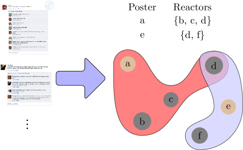
Assume $\mathcal{P}_{k}$ are all equivalent and let $\mathcal{P}_{k}=\mathbb{N}$ be a countably infinite population. An e-mail can be represented as the ordered sequence of sets: sender, receivers. Then an e-mail interaction process is a correspondence $\mathcal{I}:I\to\mathop{\text{fin}}\nolimits_{1}(\mathbb{N})\times\mathop{\text{fin}}\nolimits(\mathbb{N})$. For instance, $I(1)=(\{a\},\{b,c\})$ is an e-mail from sender $a$ to receivers $b$ and $c$. This is distinct from $(\{b\},\{a,c\})$ and $(\{c\},\{a,b\})$. Figure 1 is a visualization of a similar structured interaction dataset formed from Facebook posts (i.e., poster followed by finite multiset of responders).

Figure 1. Example of network data from Facebook posts. The post process is a correspondence $\mathcal{I}:I\to\mathop{\text{fin}}\nolimits_{1}(\mathop{\mathbb{N}}\nolimits)\times\mathop{\text{fin}}\nolimits(\mathop{\mathbb{N}}\nolimits)$. Here $I=\mathop{\mathbb{N}}\nolimits$, and the first post $\mathcal{I}(1)=\{\{a\},\{b,c,d\}\}$ represents user $a$ posting to the forum and $b,c,d$ reacting to the post. The second post $\mathcal{I}(2)=\{\{e\},\{d,f\}\}$ represents user $e$ posting to the forum and $d,f$ reacting. User $d$ reacts to both posts.

Example 2.5 (Scientific articles).

Consider summarizing a scientific article by its (1) list of subject areas and (2) list of authors. Then the scientific article process is a correspondence $\mathcal{I}:I\to\mathop{\text{fin}}\nolimits(\mathcal{P}_{1})\times\mathop{\text{fin}}\nolimits(\mathcal{P}_{2})$. For instance, $I(1)=(\{a,b\},\{c,d\})$ is an article with subject areas $a$ and $b$ and authors $c$ and $d$. Here, $\mathcal{P}_{1}$ and $\mathcal{P}_{2}$ are distinct populations.

Example 2.6 (Movies).

Consider summarizing a movie by its (1) genre, (2) list of producers, (3) director, and (4) list of actors. Of course, there is overlap in certain populations, as producers can be directors, directors can be actors, but none are a genre (unless Scorsese, Spielberg, or Tarantino are considered genres unto themselves). Then the movie process is a correspondence $\mathcal{I}:I\to\mathop{\text{fin}}\nolimits_{1}(\mathbb{N})\times\mathop{\text{fin}}\nolimits(\mathbb{N})\times\mathop{\text{fin}}\nolimits_{1}(\mathbb{N})\times\mathop{\text{fin}}\nolimits(\mathbb{N})$. For instance, $I(1)=(\{a\},\{b,c\},\{d\},\{d,e,f\})$ is a movie with genre $a$, producers $b$ and $c$, director $d$, and actors $d$, $e$, and $f$. Note, in this example, the director is also one of the actors.

The above shows Definition 2.1 covers a wide variety of examples from network science. Next, we construct interaction-labeled networks and define exchangeable structured interaction processes.

Remark 2.7 (Covariates).

In this paper, we focus on the study of structured interaction processes in Definition 2.1 with no additional information, such as covariates. Incorporating such covariate information is quite difficult; see [28, 29, 30, 31, 32, 33] for examples of incorpating covariates into network analysis. Covariate information can come in two forms: (1) covariate information on the interaction; and (2) covariate information on constituent elements. Examples of (1) include subject line or body text in an e-mail, or genre and gross movie sales for a movie. Examples of (2) include gender, age, job title, or university affiliation of authors of a scientific article. Certain interaction covariates can be incorporated into the models considered in this paper. For example, in the ArXiV dataset, the article’s subject can be viewed as covariate information on the interaction. We show how this can be incorporated as part of the structured interaction data structure, and therefore accounted for in the statistical models.

2.1. Interaction-labeled networks

For the remainder of this paper, we focus on structured interaction processes of the form $\mathcal{I}:I\to\mathop{\text{fin}}\nolimits(\mathcal{P}_{1})\times\mathop{\text{fin}}\nolimits(\mathcal{P}_{2})$. This type of a structured interaction process captures the phone-call, e-mail, and scientific article examples. The arguments presented naturally extend to more general structured interaction processes as given in Definition 2.1. When two populations of constituent elements are equivalent, we write $\mathcal{P}_{1}\equiv\mathcal{P}_{2}$. The interaction-labeled network is an equivalence clase constructed from the structured interaction process by quotienting out the labeling of the constituent elements. Let $\rho_{j}:\mathcal{P}_{j}\to\mathcal{P}_{j}^{\prime}$ be a bijection for $j=1,2$. We write $\rho:\mathcal{P}_{1}\times\mathcal{P}_{2}\to\mathcal{P}_{1}^{\prime}\times\mathcal{P}_{2}^{\prime}$ to be the composite bijection obtained by applying $\{\rho_{j}\}_{j=1,2}$ componentwise. If $\mathcal{P}_{1}\equiv\mathcal{P}_{2}$, then $\rho_{1}\equiv\rho_{2}$; that is, bijections among equivalent populations, e.g., the senders and receivers in an email network, denoted by $\bar{s}$ and $\bar{r}$, respectively, must agree. Then $\rho$ induces an action on the product space $\mathop{\text{fin}}\nolimits(\mathcal{P}_{1})\times\mathop{\text{fin}}\nolimits(\mathcal{P}_{2})$ by the composite map

$$(\bar{s},\bar{r}) =(\{s_{1},\ldots,s_{k_{1}}\},\{r_{1},\ldots,r_{k_{2}}\})\in\mathop{\text{fin}}\nolimits(\mathcal{P}_{1})\times\mathop{\text{fin}}\nolimits(\mathcal{P}_{2})$$

$$\to\rho\,(\bar{s},\bar{r}) =(\{\rho_{1}s_{1},\ldots,\rho_{1}s_{k_{1}}\},\{\rho_{2}r_{1},\ldots,\rho_{2}r_{k_{2}}\})\in\mathop{\text{fin}}\nolimits(\mathcal{P}^{\prime}_{1})\times\mathop{\text{fin}}\nolimits(\mathcal{P}^{\prime}_{2})$$

Therefore, the bijection $\rho$ acts on the structured interaction process via composition $(\rho\mathcal{I})(i)=\rho(\mathcal{I}(i)),i\in\mathbb{N}$. The structured interaction-labeled network is then the equivalence class constructed from the structured interaction network by quotienting out over bijections $\rho$:

(1) $${\bf y}_{\mathcal{I}}=\bigcup_{\begin{subarray}{c}\#\mathcal{P}_{j}^{\prime}=\#\mathcal{P}_{j}\\ j=1,2\end{subarray}}\left\{\mathcal{I}^{\prime}:I\to\mathop{\text{fin}}\nolimits(\mathcal{P}^{\prime}_{1})\times\mathop{\text{fin}}\nolimits(P^{\prime}_{2}):\rho\mathcal{I}=\mathcal{I}^{\prime}\text{ for some bijection }\rho:\mathcal{P}_{1}\times\mathcal{P}_{2}\to\mathcal{P}^{\prime}_{1}\times\mathcal{P}_{2}^{\prime}\right\},$$

where $\#\mathcal{P}_{j}$ is the cardinality of the population. Note we have only quotiented out labels for constituent elements, so the object ${\bf y}_{\mathcal{I}}$ still has uniquely labeled interactions. For simplicity, we write ${\bf y}$ and leave the subscript $\mathcal{I}$ implicit.

In the remainder of the paper, we assume the index set $I$ is countably infinite and replace it by $\mathbb{N}$. For any $S\subset\mathbb{N}$, we define the restriction of $\mathcal{I}:\mathbb{N}\to\mathop{\text{fin}}\nolimits(\mathcal{P}_{1})\times\mathop{\text{fin}}\nolimits(\mathcal{P}_{2})$ to the subset $S\subset\mathbb{N}$ by $\mathcal{I}|_{S}$. This restricted interaction process induces a restriction to $S$ of the interaction-labeled network. We write ${\bf y}_{S}$ to denote the interaction-labeled network associated with the restricted process $\mathcal{I}|_{S}$. For $S=[n]:=\{1,\ldots,n\}$, we simply write $\mathcal{I}_{n}$ to denote the restricted structured interaction process and ${\bf y}_{n}$ to denote the corresponding structured interaction network.

3. Structured interaction exchangeable models

Let ${\bf y}$ denote the interaction-labeled network constructed from the structured interaction process $\mathcal{I}:\mathbb{N}\to\mathop{\text{fin}}\nolimits(\mathcal{P}_{1})\times\mathop{\text{fin}}\nolimits(\mathcal{P}_{2})$. Then for any finite permutation $\sigma:\mathbb{N}\to\mathbb{N}$, let $\mathcal{I}^{\sigma}$ denote the relabeled structured interaction process defined by  $\mathcal{I}^{\sigma}(i)=\mathcal{I}(\sigma^{-1}(i)),i\in\mathbb{N}$. Then ${\bf y}^{\sigma}$ denotes the corresponding interaction labeled network constructed from $\mathcal{I}^{\sigma}$. Note that the choice of representative from the equivalence class does not matter. The above relabeling by permutation $\sigma$ is not to be confused with the relabeling in the previous section by the bijection $\rho$. The bijection $\rho$ relabels the constituent elements, and is used to construct the equivalence class defining the interaction-labeled network (i.e., the equivalence class). The permutation $\sigma$ reorders the interaction process, and therefore relabels the interaction-labeled network.

In the remainder of this paper, we write ${\bf Y}$ to denote a random interaction-labeled network. We assume the interactions are labeled in the countably infinite set $\mathop{\mathbb{N}}\nolimits$. Interaction exchangeability is characterized by the property that the labeling of the interactions (not the constituent elements) is arbitrary. We now define exchangeable structured interaction networks.

Definition 3.1 (Exchangeable structured interaction network process).

The structured interaction-labeled network ${\bf Y}$ is exchangeable if ${\bf Y}^{\sigma}=_{\mathcal{D}}{\bf Y}$ for all permutations $\sigma:\mathop{\mathbb{N}}\nolimits\to\mathop{\mathbb{N}}\nolimits$, where $=_{\mathcal{D}}$ denotes equality in distribution.

Next, we provide a representation theorem for structured interaction processes. We focus on the setting where each interaction $(\bar{s},\bar{r})$ is either never observed or observed infinitely often. This is commonly referred to as the “blip-free” setting [34], where blips refer to interactions $(\bar{s},\bar{r})$ that are observed once. We first define the $\mathop{\text{fin}}\nolimits(\mathcal{P}_{1})\times\mathop{\text{fin}}\nolimits(\mathcal{P}_{2})$-simplex

$$\mathcal{F}=\left\{(f_{(\bar{s},\bar{r})})_{(\bar{s},\bar{r})\in\mathop{\text{fin}}\nolimits(\mathcal{P}_{1})\times\mathop{\text{fin}}\nolimits(\mathcal{P}_{2})}\quad\text{and}\quad\sum_{(\bar{s},\bar{r})\in\mathop{\text{fin}}\nolimits(\mathcal{P}_{1})\times\mathop{\text{fin}}\nolimits(\mathcal{P}_{2})}f_{(\bar{s},\bar{r})}=1\right\}$$

where $(\bar{s},\bar{r}):=(\{s_{1},\ldots,s_{k_{1}}\},\{r_{1},\ldots,r_{k_{2}}\})$ for $s_{1},\ldots,s_{k_{1}}\in\mathcal{P}_{1}$ and $r_{1},\ldots,r_{k_{2}}\in\mathcal{P}_{2}$. Let $\phi$ be a probability measure on the simplex and define $f\sim\phi$ to be a random variable drawn from this measure. Then, given $f\in\mathcal{F}$, let the sequence of interactions $\mathcal{I}(1),\mathcal{I}(2),\ldots$ be generated according to

(2) $$\mathop{\text{pr}}\nolimits\left(\mathcal{I}(i)=\left(\{s_{1},\ldots,s_{k_{1}}\},\{r_{1},\ldots,r_{k_{2}}\}\right)\,|\,f\right)=f_{(\bar{s},\bar{r})}.$$

Then, given $\mathcal{I}$, set ${\bf Y}={\bf y}_{\mathcal{I}}$. Theorem 3.2 states that all blip-free structured interaction exchangeable networks can be generated in this manner. The proof can be found in Section LABEL:section:rep of the supplementary materials.

Theorem 3.2 (Blip-free representation theorem).

Let ${\bf Y}$ be a structured interaction exchangeable network that is blip-free with probability 1. Then there exists a probability measure $\phi$ on $\mathcal{F}$ such that ${\bf Y}\sim\epsilon_{\phi}$, where

$$\epsilon_{\phi}(\cdot)=\int_{\mathcal{F}}\epsilon_{f}(\cdot)\phi(df).$$

3.1. Hierarchical vertex components model

Via Theorem 3.2, we can construct a particular family of interaction exchangeable random networks as follows. First, choose a distribution of senders, $f^{\prime}=(f_{s})_{s\in\mathcal{P}_{1}}$, in the simplex

$$\mathcal{F}_{1}:=\left\{(f_{s})_{s\in\mathcal{P}_{1}}:f_{s}\geq 0\quad\text{and}\quad\sum_{s\in\mathcal{P}_{1}}f_{s}=1\right\}.$$

Next, choose a second element of $\mathcal{F}_{1}$, which we denote $w$. Finally, for each $s\in\mathcal{P}_{1}$, construct a conditional distribution over the receivers, i.e., the second component $\mathop{\text{fin}}\nolimits(\mathcal{P}_{2})$. That is, for every $s\in\mathcal{P}_{1}$, we choose $f^{\prime\prime}_{s}=(f_{r\,|\,s})_{r\in\mathcal{P}_{2}}$ in the simplex

$$\mathcal{F}_{2}=\left\{(f_{r})_{r\in\mathcal{P}_{2}}:f_{r}\geq 0\quad\text{and}\quad\sum_{r\in\mathcal{P}_{2}}f_{r}=1\right\}.$$

We combine these distributions to form $f\in\mathcal{F}_{1}\times\mathcal{F}_{1}\times(\otimes_{s\in\mathcal{P}_{1}}\mathcal{F}_{2})$, which determines a distribution on the space $\mathop{\text{fin}}\nolimits_{1}(\mathcal{P}_{1})\times\mathop{\text{fin}}\nolimits(\mathcal{P}_{2})$ by

(3) $$\mathop{\text{pr}}\nolimits\left(E=(\bar{s},\bar{r})\mid f\right)=\nu_{k_{1}}\left[\prod_{i=1}^{k_{1}}f_{s_{i}}\right]\cdot\frac{\sum_{i=1}^{k_{1}}w_{s_{i}}\cdot\nu^{(s_{i})}_{k_{2}}\left[\prod_{j=1}^{k_{2}}f_{r_{j}\,|\,s_{i}}\right]}{\sum_{i=1}^{k_{1}}w_{s_{i}}},$$

where $\nu_{l}\geq 0$, $\nu^{(s)}_{l}\geq 0$, $\sum_{l=1}^{\infty}\nu_{l}=1$, and $\sum_{l=1}^{\infty}\nu_{l}^{(s)}=1$ for each $s\in\mathcal{P}_{1}$. This determines an interaction exchangeable network, which we call the hierarchical vertex components model (HVCM). Given $f$, $\mathcal{I}(1),\mathcal{I}(2),\ldots$ are independent, identically distributed (i.i.d.) random structured interactions drawn from (3). The associated random interaction exchangeable network ${\bf Y}:={\bf y}_{\mathcal{I}}$ is obtained through (1), whose distribution we denote by $\epsilon_{f}$.

In non-HVCMs [35], each constituent element had a single frequency of occurrence. By contrast, HVCMs allow the frequency of occurrence for elements in the second term of (3) (i.e., $r\in\mathcal{P}_{2}$) to depend on first component (i.e., $\bar{s}\in\mathop{\text{fin}}\nolimits\mathcal{P}_{1}$) through $f_{r|s}$. This dependence is two-fold: (1) $w\in\mathcal{F}_{1}$ controls which $f^{\prime\prime}_{s}$ is chosen across $s\in\bar{s}$; and (2) the local distributions can vary, leading to the size-biased ordering of $r\in\mathcal{P}_{2}$ varying as a function of $s$.

Remark 3.3 (Vertex exchangeability versus interaction exchangeability).

While HVCMs are expressed as a function of the vertices, they are interaction exchangeable and not vertex exchangeable. To see this, consider Theorem 3.2. A direct corollary is that vertices are sampled in size-biased order according to their relative frequency of occurrence. In hierarchical models, the size-biased sampling of the second component depends on the first component. Regardless, this implies the observed constituent elements are not exchangeable with the unobserved constituent elements. On the other hand, vertex exchangeability implicitly assumes the observed vertices and unobserved vertices are exchangeable.

4. Sequential description for particular subfamily of HVCMs

Here we provide a sequential description of a particular subfamily of HVCMs. For ease of comprehension, we start with the setting of a single sender where the size of the first component is one (i.e., $\nu_{k_{1}}=1[k_{1}=1]$). In this setting, the sequential description is presented in the context of e-mails. Let $(\tilde{\alpha},\tilde{\theta})$ satisfy either (1) $0\leq\tilde{\alpha}<1$ and $\tilde{\theta}>0$, or (2) $\tilde{\alpha}<0$ and $\theta=-K\tilde{\alpha}$ for some $K\in\mathbb{N}$. In setting (1), the population $\mathcal{P}_{1}$ is infinite, while in setting (2) the population is finite and equal to $K$. In Section 4.3, we show how to extend this model to the general setting of multiple senders. For ease of comprehension, we let $\mathcal{S}=\mathcal{P}_{1}$ (senders) and $\mathcal{R}=\mathcal{P}_{2}$ (receivers) denote the two sets of constituent elements.

We introduce some additional notation. For each $n=1,2,\ldots$, the $n$th email $E_{n}$ is given by the structured interaction $(\bar{S}_{n},\bar{R}_{n})=(\{S_{n,1}\},\{R_{n,1},\ldots,R_{n,k_{n,2}}\})$ where $S_{n,1}\in\mathcal{S}$ is the sender, and $R_{n,j}\in\mathcal{R}$ is the $j$th receiver of the $n$th article. Suppose $n$ articles have been observed and define $\mathcal{H}_{n}=\left\{E_{1},\ldots,E_{n}\right\}$ to be the observed history of the first $n$ e-mails. For the $(n+1)$st e-mail, choose the sender according to

(4) $$\mathop{\text{pr}}\nolimits\left(S_{n+1,1}=s\,|\,\mathcal{H}_{n}\right)\propto\left\{\begin{array}[]{c c}D^{out}_{n}(s)-\tilde{\alpha}&s\in\mathcal{S}_{n}\\ \tilde{\theta}+\tilde{\alpha}|\mathcal{S}_{n}|&s\not\in\mathcal{S}_{n}.\end{array}\right.$$

where $D_{n}^{out}(s)$ is the outdegree of the subject $s$, and $\mathcal{S}_{n}$ are the set of unique senders in $(\bar{S}_{1},\ldots,\bar{S}_{n})$ and $|\mathcal{S}_{n}|$ is the set’s cardinality.

Given $S_{n+1,1}=s\in\mathcal{S}$, we choose the number of recipients according to the discrete probability distribution function $\{\nu_{k}^{(s)}\}_{k=1}^{\infty}$. Finally, let $D_{n,j}(s,r)$ denote the indegree of receiver $r$ when restricted to e-mails from sender $s$ after the first $n$ e-mails and the $j-1$ recipients of the $n$th e-mail; that is,

$$D_{n,j}(s,r)=\#\,\{(m,l)\,|\,R_{m,l}=r\text{ and }S_{m,1}=s\text{ for }m<n\;\text{and}\;l\leq k_{m}\text{, or }m=n\;\text{and}\;l<j\}.$$

Finally, we define $m_{n,j}(s)=\sum_{r\in\mathcal{R}}D_{n,j}(s,r)$ to be the number of receivers (accounting for multiplicity) of e-mails from sender $s$. Each of these statistics is a measurable function of $\mathcal{H}_{n}$. Note, these statistics are local (i.e., specific to the particular subject). Here, we describe a procedure for sharing information across senders. To do this, we define a partially observable global set of information. First, define the observable variable $R_{n,j}$ to be the complete set of receivers; that is,

$$R_{n,j}=\{r\in\mathcal{R}\,|\,\exists\,R_{m,l}=r\text{ for }m<n\,\text{and}\,l\leq k_{m}\text{, or }m=n\,\text{and}\,l<j\}.$$

Additionally, let $K_{n,j}=|R_{n,j}|$ be the cardinality of this set. For each $r\in R_{n,j}$ we posit existence of a latent degree per sender $s\in\mathcal{S}_{n}$ and receiver $r$ denoted by $V_{n,j}(s,r)$. We then define $V_{n,j}(\cdot,r)=\sum_{s\in\mathcal{S}_{n}}V_{n,j}(s,r)$ and $m_{n,j}=\sum_{r\in\mathcal{R}_{n,j}}V_{n,j}(\cdot,r)$. Next, define $R_{n,j}(s)$ to be the complete set of receivers when restricting to e-mails from sender $s\in\mathcal{S}_{n}$, and $\mathcal{H}_{n,j}$ to be the observable history $\mathcal{H}_{n-1}$ union $\{S_{n,1},R_{n,1},\ldots,R_{n,j}\}$. That is, $\mathcal{H}_{n,j}$ is the observed history up to the $j-1$th receiver on the $n$th e-mail, where $\mathcal{H}_{n,0}$ implies only sender information for the $n$th e-mail. Finally, for each $s\in\mathcal{S}$, let $(\alpha_{s},\theta_{s})$ satisfy either (1) $0\leq\alpha_{s}<1$ and $\theta>0$, or (2) $\alpha_{s}<0$ and $\theta_{s}=-K^{\prime}\alpha_{s}$ for some $K^{\prime}\in\mathbb{N}$. In setting (1), the receiver population $\mathcal{P}_{2}$ is infinite, while in setting (2) the population is finite and equal to $K^{\prime}$. For the remainder of this paper, we assume setting (1).

Given the indegree distribution $\{D_{n,j}(s^{\prime},r^{\prime})\}_{r^{\prime}\in R_{n,j},s^{\prime}\in\mathcal{S}_{n}}$, the latent degree distribution  $\{V_{n,j}(s^{\prime},r^{\prime})\}_{r^{\prime}\in R_{n,j},s^{\prime}\in\mathcal{S}_{n}}$, the current sender $s$, along with the observable history $\mathcal{H}_{n,j}$, the probability of choosing receiver $r$ is proportional to

(5) $$\frac{D_{n,j}(s,r)-\alpha_{s}V_{n,j}(s,r)+(\theta_{s}+\alpha_{s}V_{n,j}(s,r))\left(\frac{V_{n,j}(\cdot,r)-\alpha}{m_{n,j}+\theta}\right)}{m_{n,j}(s)+\theta_{s}},r\in R_{n,j}(s)$$

and

(6) $$\frac{\theta_{s}+\alpha_{s}V_{n,j}(s,r)}{m_{n,j}(s)+\theta_{s}}\cdot\frac{\theta+\alpha V_{n,j}(\cdot,r)}{m_{n,j}+\theta},r\not\in R_{n,j}(s).$$

Note the difference in the discount of indegree in (5) and outdegree in (4). For the sender distribution (4), the outdegree discount is $\tilde{\alpha}$; on the other hand, for (5), the indegree discount is $\alpha_{s}V_{n,j}(s,r)$. This reflects that in (4), sender $s$ is chosen from a single distribution; however, in (5), receiver $r$ can be chosen either locally or globally.

The remaining question is how to update the degree distributions. In (5) and (6), we can either observe $r$ “locally”, or we escape the local model and observe $r$ due to the latent global information. Given $R_{n,j}=r$ we update both local and global degrees. If $r\not\in R_{n,j}(s)$ then the global degree $V_{n,j}(s,r)$ increases from zero to one. If $r\in R_{n,j}(s)$ then the local degree $D_{n,j}(s,r)$ increases by one and the latent degree is increased by one with probability $\tau_{n,j}(s)=\frac{\theta_{s}+\alpha_{s}V_{n,j}(s,r)}{m_{n,j}(s)+\theta_{s}}$. The exact procedure for incrementing $V_{n,j}$ is discussed in section 6.

4.1. Partial pooling

The importance of the latent global degree distribution is that it allows information to be shared across the conditional receiver distributions. The above model formalizes the partial pooling of information. The degree of pooling is controlled by the escape probability $\tau_{n,j}(s)$, which in general decreases as the number of e-mails from sender $s$ increases. Note that over time as more e-mails by sender $s$ are seen, the escape probability $\tau_{n,j}(s)$ tends to zero whenever $\alpha_{s}<1$. Therefore, the local impact of the latent global degree information becomes negligible once we have sufficient local information. However, the first time a sender-receiver pair is observed, it must occur via the shared global set of information. The global latent degrees $\{V_{n,j}(s,r)\}_{r\in R_{n,j},s\in S_{n}}$ therefore contribute to the behavior of new and/or rarely seen senders.

4.2. Connection between sequential description and hierarchical vertex components models

The sequential description in section 6 is equivalent to a particular HVCM. When $\alpha_{s}=0,~{}\forall s\in\mathcal{P}_{1}$, an analytic stick-breaking representation can be derived. This connects the sequential process directly to (3). To do so, we start by constructing the sender distribution. Here, we assume $\mathcal{P}_{1}\equiv\mathcal{P}_{2}\equiv\mathop{\mathbb{N}}\nolimits$. For $s\in\mathbb{N}$, define independent random variables $\beta_{s}\sim\text{Beta}(1-\tilde{\alpha},\tilde{\theta}+s\tilde{\alpha})$. Then, conditional on $\{\beta_{s}\}_{s=1}^{\infty}$, the probability of choosing sender $s\in\mathbb{N}$ is given by

$$f_{s}\,|\,\{\beta_{s^{\prime}}\}_{s^{\prime}=1}^{\infty}=\beta_{s}\prod_{i=1}^{s-1}(1-\beta_{i}),$$

where the product is set equal to one for $s=1$, and $f^{\prime}=\{f_{s}\}_{s=1}^{\infty}$. In our current setting, $\nu_{k_{1}}=1[k_{1}=1]$ so the weights $w=\{w_{s}\}_{s=1}^{\infty}$ can be ignored for now. See Section 4.3 for a description of how these can be constructed in a similar manner.

We now construct, for each $s\in\mathbb{N}$ the probabilities $\{f_{r\,|\,s}\}_{r=1}^{\infty}$ via a hierarchical model given $\alpha>0$ and $\theta>-\alpha$, and we set $f^{\prime\prime}=\{\{f_{r|s}\}_{r=1}^{\infty}\}_{s=1}^{\infty}$ . To do this, we first define global independent random variables $\tilde{\beta}_{r}\sim\text{Beta}(1-\alpha,\theta+r\alpha)$ for $r\in\mathbb{N}$. Then, conditional on $\{\tilde{\beta}_{r}\}_{r=1}^{\infty}$, for $r\in\mathbb{N}$, we define associated stick-breaking probabilities $\tilde{\pi}_{r}=\tilde{\beta}_{r}\prod_{i=1}^{r-1}(1-\tilde{\beta}_{i})$. These are probabilities of choosing receiver $r$ based on the global random variables $\{\tilde{\beta}\}_{r=1}^{\infty}$. The local stick-breaking distributions are then defined via a perturbation of these global probabilities. That is, for $\theta_{s}>0$, define independent random variable

$$\tilde{\beta}^{\prime}_{r\,|\,s} \sim\text{Beta}\left(\theta_{s}\tilde{\pi}_{r},\theta_{s}\left(1-\sum_{l=1}^{r}\tilde{\pi}_{l}\right)\right)$$

$$f_{r\,|\,s}\,|\,\{\tilde{\beta}^{\prime}_{j\,|\,s}\}_{j=1}^{\infty} =\tilde{\beta}^{\prime}_{r\,|\,s}\prod_{i=1}^{r-1}\left(1-\tilde{\beta}_{i\,|\,s}^{\prime}\right)$$

where the product is defined equal to one when $r=1$. This yields a stick breaking representation for $f=\{f^{\prime},f^{\prime\prime}\}$ for a particular hierarchical vertex components model. Partial pooling occurs via the shared global probabilities $\tilde{\pi}_{r}$. The local distributions satisfy $\mathbb{E}\left[f_{r\,|\,s}\,|\,\{\tilde{\pi}_{r^{\prime}}\}_{r^{\prime}=1}^{\infty}\right]=\pi_{r}$. Therefore, the distribution $\{f_{r\,|\,s}\}_{r=1}^{\infty}$ can be thought of as perturbation of the global distribution $\{\pi_{r}\}_{r=1}^{\infty}$ where $\theta_{s}$ controls the amount of perturbation. In particular, $f_{r\,|\,s}\to\pi_{r}$ with probability one as $\theta_{s}\to\infty$.

By construction, $f=(\{f_{s}\}_{s=1}^{\infty},\{f_{r\,|\,s}\}_{s,r=1}^{\infty})$ is a random variable over the space $\mathcal{F}_{1}\times\otimes_{s=1}^{\infty}\mathcal{F}_{2}$. Lemma 4.1 establishes the connection between these random variables and the canonical model for $\alpha_{s}=0$. Although this model for $\alpha_{s}>0$ does not admit a known stick breaking representation, Theorem 3.2 discussed in Section 3 ensures these asymptotic frequencies exist. Section LABEL:appendix:technical of the supplementary materials describes a specific probabilistic construction of these frequencies.

Lemma 4.1.

The sequential HVCM model for $\alpha_{s}=0$ for $s\in\mathbb{N}$ is equivalent in distribution to (3), where $f$ is distributed according to the stick-breaking construction described above.

Proof can be found in section LABEL:appendix:technical of the supplementary materials; see [36, 37] for further details on the stick-breaking representation.

Remark 4.2 (Connections to CRFP).

Note that the HVCM described above is closely related to the Chinese Restaurant Franchise Process, a well-known process in the machine learning literature [36, 38] that is almost exclusively used to model latent clusters in data. Here, we use these ideas in the construction of the interaction process. Thus, the objectives are quite different; for instance, there is almost no focus on the inference of the model parameters in the ML community; in our setting, these parameters are crucial to understanding the overall interaction process behavior. This model is most similar to [39], where it is used for language modeling. Similar to the CFRP, the above construction is related to the Pitman-Yor process and the GEM distributions [36]. More details can be found in Section6 and the supplementary materials.

4.3. Accounting for multiple elements in first component

In the general setting, the first component, $\bar{S}_{n}$, is a random element of $\mathop{\text{fin}}\nolimits(\mathcal{P}_{1})$ (i.e., a random finite multiset of elements from $\mathcal{P}_{1}$). In the sequential description, we assumed the size of this multiset was one. We now consider $\bar{S}_{n}=\{S_{n,1},\ldots,S_{n,k_{n,1}}\}$ for general $k_{n,1}\geq 1$. First, let $\mathcal{H}^{(s)}_{n,j}=\mathcal{H}_{n}\cup\{S_{n+1,1},\ldots,S_{n+1,j}\}$ denote the history of the first $n$ e-mails and the first $j$ senders of the $n+1$st e-mail. Extension of 4 to handle multiple senders is straightforward by replacing $\mathcal{H}_{n}$ by $\mathcal{H}_{n,j}^{(s)}$ and defining all other terms similarly.

In the sequential description, the sender $S_{n,1}$ is used to specify which local statistics (i.e., $V_{n,j}(r,s)$, $D_{n,j}(r,s)$ and $m_{n,j}(s)$) to consider. However, when there are multiple senders, this choice is no longer straightforward. To address this, we introduce a random variable $Z_{n}$ with domain $\bar{S}_{n}$. This variable indicates which local statistics will be used in receiver distributions (i.e., equations (5) and (6)). Define $\mathcal{S}^{(z)}_{n}$ to be the unique elements in $\mathcal{H}^{(z)}_{n}:=(Z_{1},\ldots,Z_{n})$. Then

(7) $$\mathop{\text{pr}}\nolimits\left(Z_{n}=s\,|\,\mathcal{H}^{(z)}_{n},\bar{S}_{n}\right)\propto{\bf 1}\left\{\begin{array}[]{c c}D^{(z)}_{n}(s)-\tilde{\alpha}_{z}&s\in\mathcal{S}_{n}^{(z)}\cap\bar{S}_{n}\\ \tilde{\theta}_{z}+\tilde{\alpha}_{z}|\mathcal{S}^{(z)}_{n}|&s\not\in\mathcal{S}^{(z)}_{n}\cap\bar{S}_{n}\\ 0&s\not\in\bar{S}_{n}\end{array}\right.$$

where (1) $0<\tilde{\alpha}_{z}<1$ and $\tilde{\theta}_{z}>0$ if the population $\mathcal{S}$ is considered infinite, and (2) $\tilde{\alpha}_{s}<0$ and $\tilde{\theta}_{z}=-K\tilde{\alpha}_{z}$ if population is finite and $|\mathcal{S}|=K$. This is equivalent to restricting (4) to be non-zero only on the domain $\bar{S}_{n}$. Moreover, it is conditional on the history $\mathcal{H}^{(z)}_{n}$ instead of $\mathcal{H}_{n}$. If $Z_{n}=s$ for $s\in\mathcal{S}^{(z)}_{n}$, then increase $D_{n}^{(z)}(s)$ by one. If $s\not\in\mathcal{S}_{n}$, then set $D_{n}^{(z)}(s)=1$.

5. Statistical properties

We now state several theoretical results for the proposed HVCM built from the sequential description in section 4. For ease of comprehension, we refer to this model as the “canonical HVCM model”.

Theorem 5.1.

The canonical HVCM with parameters $\Psi=(\tilde{\alpha},\tilde{\theta},\alpha,\theta,\{\alpha_{s},\theta_{s}\}_{s\in\mathcal{P}_{1}})$ determines a structured exchangeable interaction probability distribution for all $\Psi$ in the parameter space.

Theorem 5.1 is not immediate from the sequential construction in section 4, but is clear from the reparameterization of the model presented in section 6, and its connection to the model previously discussed (this is formalized in section LABEL:appendix:technical) of the supplementary materials.

The remainder of this section focuses on the setting where the size of the first component is one (i.e., $\nu_{k_{1}}=1[k_{1}=1]$). Moreover, we will make certain alternative assumptions concerning the sender distributions. These constraints allow sufficient complexity to be interesting, but assume sufficient regularity to push through the theoretical analysis. First, we turn to the growth rates in the expected number of unique receivers. Unlike the Hollywood model, this rate depends on both the distribution over senders, the global parameter $\alpha$, and the local parameters $\{\alpha_{s}\}_{s\in\mathcal{P}_{1}}$. Before stating the theorem, we require a formal definition of sparsity. For clarity, we define quantities in terms of receivers to distinguish vertices observed as senders and those observed as receivers (i.e., in $\mathcal{P}_{1}$ and $\mathcal{P}_{2}$ respectively).

For a structured interaction-labeled network ${\bf Y}$, let $v({\bf Y})$ denote the number of non-isolated receivers; $e({\bf Y})$ is the number of interactions; $M_{k}({\bf Y})$ is the number of interactions with $k$ receivers; $N_{k}({\bf Y})$ is the number of receivers that appear exactly $k$ times; and $d({\bf Y})=(d_{k}({\bf Y}))_{k\geq 1}$ is the indegree distribution, where $d_{k}({\bf Y})=N_{k}({\bf Y})/v({\bf Y})$. Note that these are global statistics that do not depend on the interaction labels. We define local versions by superscripting each statistic by $s\in\mathcal{P}_{1}$. For instance, $v^{(s)}({\bf Y})$ is the number of non-isolated receivers when restricting ${\bf Y}$ to only those interactions involving sender $s$. The statistics $e^{(s)}({\bf Y}),M^{(s)}_{k}({\bf Y}),N^{(s)}_{k}({\bf Y}),d^{(s)}({\bf Y})$ and $d_{k}^{(s)}({\bf Y})$ are defined similarly.

Definition 5.2 (Global and local sparsity).

Let $({\bf Y}_{n})_{n\geq 1}$ be a sequence of interaction-labeled networks for which $e({\bf Y}_{n})\to\infty$ as $n\to\infty$. The sequence $({\bf Y}_{n})_{n\geq 1}$ is sparse if

$$\limsup_{n\to\infty}\frac{e({\bf Y}_{n})}{v({\bf Y}_{n})^{m_{\bullet}({\bf Y}_{n})}}=0,$$

where $m_{\bullet}({\bf Y}_{n})=e({\bf Y}_{n})^{-1}\sum_{k\geq 1}kM_{k}({\bf Y}_{n})$ is the average arity (i.e., number of receivers) of the interactions in $\mathcal{E}_{n}$. A non-sparse network is  dense. We say the sequence is $(\mathcal{E}_{n})_{n\geq 1}$ is $s$-locally sparse if

$$\limsup_{n\to\infty}\frac{e^{(s)}({\bf Y}_{n})}{v^{(s)}({\bf Y}_{n})^{m^{(s)}_{\bullet}({\bf Y}_{n})}}=0,$$

where $m^{(s)}_{\bullet}({\bf Y}_{n})=e^{(s)}({\bf Y}_{n})^{-1}\sum_{k\geq 1}kM^{(s)}_{k}({\bf Y}_{n})$ is the average arity (i.e., number of receivers) of the interactions in ${\bf Y}_{n}$ from sender $s\in\mathcal{P}_{1}$. A network that is not $s$-locally sparse is $s$-locally dense.

For $(X_{n})_{n\geq 1}$ a sequence of positive random variables and $(y_{n})_{n\geq 1}$ a sequence of positive non-random variables, let $X_{n}\simeq y_{n}$ indicate $\lim_{n\to\infty}X_{n}/y_{n}$ exists almost surely and equals a finite and positive random variable. Theorem 5.3 shows the canonical model may be either globally sparse and/or dense. The theorem assumes a finite population of senders with number of e-mails per sender drawn from a multinomial distribution.

Theorem 5.3.

Suppose the sender population $\mathcal{P}_{1}$ is finite, consisting of $d$ senders, i.e., $\mathcal{P}_{1}=[d]:=\{1,\ldots,d\}$. Assume, out of the $n$ e-mails, the number of e-mails per sender $s$, denoted $n_{s}$, is drawn from a multinomial distribution with probabilities $(p_{1},\ldots,p_{d})$ such that $\sum_{s=1}^{d}p_{s}=1$ and $p_{s}>0$ for all $s\in[d]$. Let $\mu_{s}$ be the average size of emails for sender $s$ and $\mu:=\sum_{s=1}^{d}p_{s}\mu_{s}$ the average size of emails across all senders. Then $v({\bf Y}_{n})\simeq(\mu^{1/\alpha_{\star}}\mu_{\star}p_{\star}n)^{\alpha_{0}\alpha_{*}}$ where $s^{\star}=\arg\max_{s\in[d]}\alpha_{s}$, $\mu_{\star}=\mu_{s^{\star}}$, and $\alpha_{\star}=\alpha_{s^{\star}}$. In particular, if $\mu^{-1}<\alpha\cdot\alpha_{\star}<1$, then $({\bf Y}_{n})_{n\geq 1}$ is almost surely sparse.

Theorem 5.3 establishes that the canonical HVCM for a special case of the sender distribution can capture degrees of sparsity. If $\mu_{s}=\mu$ for all $s\in\mathcal{P}_{1}$ and $\alpha\alpha_{\star}<\mu^{-1}$ then it must be the case that $\alpha\alpha_{s}<\mu^{-1}$ for all $s\in\mathcal{P}_{1}$. Therefore, a dense network must be $s$-locally dense for all $s\in\mathcal{P}_{1}$. However, a sparse network can be $s$-locally dense for some, but not all, $s\in\mathcal{S}$. We turn now to considerations of power-law degree distribution for interaction-labeled networks. We start with a definition.

Definition 5.4 (Global power-law degree distributions).

A sequence $({\bf Y}_{n})_{n\geq 1}$ exhibits power-law degree distribution [7, 23, 24] if for some $\gamma>1$ the degree distributions $(d({\bf Y}_{n}))_{n\geq 1}$ satisfy $d_{k}({\bf Y}_{n})\sim l(k)k^{\gamma}$ as $n\to\infty$ for all large $k$ for some slowly varying function $l(x)$; that is, $\lim_{x\to\infty}l(tx)/l(x)=1$ for all $t>0$, where $a_{n}\sim b_{n}$ indicates that $a_{n}/b_{n}\to 1$ as $n\to\infty$. More precisely, $({\bf Y}_{n})_{n\geq 1}$ has power law degree distribution with index $\gamma$ if

(8) $$\lim_{k\to\infty}\lim_{n\to\infty}\frac{d_{k}({\bf Y}_{n})}{l(k)k^{-\gamma}}=1.$$

Theorem 5.5 establishes the power-law degree distribution for the canonical HVCM for the case of $\alpha_{s}=1,\forall s\in\mathcal{S}$.

Theorem 5.5.

Let $({\bf Y}_{n})_{n\in\mathbb{N}}$ obey the sequential description in section 4 with parameters $(\tilde{\alpha},\tilde{\theta})$ and let $\alpha_{s}=1$ for all $s\in\mathcal{P}_{1}$. For each $n\geq 1$, let $p_{n}(k)=N_{k}(\mathcal{Y}_{n})/v(\mathcal{E}_{n})$ for $k\geq 1$ be the empirical receiver degree distribution where $N_{k}(\mathcal{E}_{n})$ is the number of receivers of degree $k\geq 1$ and $v(\mathcal{E}_{n})$ is the number of unique receivers in $\mathcal{E}_{n}$. Then, for every $k\geq 1$,

(9) $$p_{n}(k)\sim\alpha k^{-(\alpha+1)}/\Gamma(1-\alpha)$$

where $\Gamma(t)=\int_{0}^{\infty}x^{t-1}e^{-x}dx$ is the gamma function. That is, $(\mathcal{Y}_{n})_{n\geq 1}$ has a power law degree distribution with exponent $\gamma=1+\alpha\in(1,2)$.

6. Posterior inference

We now consider performing posterior inference for the canonical HVCM given an observed interaction network ${\bf Y}_{n}$. As in Section 4, we start with the setting where the size of the first component is one (i.e., $\nu_{k_{1}}=1[k_{1}=0]$). The parameters $(v^{(s)}_{k_{2}})_{~{}k_{2}\in\mathbb{N}},$ for all $s\in\mathcal{S}$ are estimated non-parametrically, and are not important for the remainder of the paper; therefore, the details are omitted for these parameters.

We start by reparameterizing the HVCM in a more useful form for inference, and which gives an explicit structure for updating the latent degree $V_{n,j}$ - we call this the extended canonical HVCM, or extended model for short. In this representation, every “escape” from the local distribution and choice of receiver $r$ leads to an auxiliary vertex $v$ being introduced locally for a sender $s$ - auxiliary vertices are not shared between senders. The label $l_{s}(v)$ of the auxiliary vertex is $r$; the auxiliary vertex accounts for the fact that the global distribution can select receiver $r$ multiple times. Finally, the observed reciever is assigned to the auxiliary vertex, and we write that assignment $\phi_{n,j}=v.$ The number of auxiliary vertices with label $r$ and sender $s$ is equal to the number of times the local distribution for sender $s$ escapes and choose the global set of information (i.e., $V_{n,j}(r,s)$). The sum of the degrees across auxiliary vertices with label $r$ and sender $s$ is equal to the indegree for receiver $r$ (i.e., $D_{n,j}(r,s)$). Finally, we write $d_{srv}$ to denote the degree of auxiliary vertex $v$ in sender $s$ that also has label $r$. Note that for $r^{\prime}\neq l_{s}(v),~{}d_{srv}=0$.

Given $\mathcal{H}_{n}$ and $S_{n+1,1}=s$, the probability that $R_{n+1,j}$ is assigned to auxiliary vertex $\phi_{n+1,j}=v$ is:

$$\mathop{\text{pr}}\nolimits(\phi_{n+1,j}=v\,|\,\mathcal{H}_{n},S_{n+1,1}=s)\propto\begin{cases}d_{s\cdot v}-\alpha_{s},&v\leq V_{n+1,j}(s,\cdot)\\ \alpha_{s}V_{n+1,j}(s,\cdot)+\theta_{s},&v=V_{n+1,j}(s,\cdot)+1,\end{cases}$$

Further, if $\phi_{n+1,j}=V_{n+1,j}(s,\cdot)+1$, then we add an auxiliary vertex $V_{n+1,j}(s,\cdot)+1$ with its label chosen with probability:

$$\mathop{\text{pr}}\nolimits(l_{s}(V_{n+1,j}+1)\,|\,\phi_{n+1,j}=V_{n+1,j}(s,\cdot)+1,\mathcal{H}_{n,j},S_{n+1}=s)\propto\begin{cases}V_{n,j}(\cdot,r)-\alpha,&r\in\mathcal{R}_{n+1,j}\\ \alpha V_{n+1,j}(\cdot,r)+\theta,&r\notin\mathcal{R}_{n+1,j}.\end{cases}$$

The likelihood of observing ${\bf Y}_{N}=\{\{S_{n,1},k_{n},\{R_{n,j},\phi_{n,j}\}_{j=1}^{k_{n}}\},\{l_{s}(\cdot)\}_{s\in\mathcal{S}_{N}}\}_{n=1}^{N}$ given the parameters $\Psi=(\tilde{\alpha},\tilde{\theta},\alpha,\theta,\{\alpha_{s},\theta_{s}\}_{s\in\mathcal{P}_{1}})$ is given by

(10) $$\mathop{\text{pr}}\nolimits({\bf Y}_{N})=\mathop{\text{pr}}\nolimits(\{\{R_{n,j}\}_{j=1}^{k_{n}}\}_{n=1}^{N},{l_{s}(\cdot)}_{s\in\mathcal{S}_{N}}|\{S_{n,1}\}_{n=1}^{N},\{k_{n}\}_{n=1}^{N})\mathop{\text{pr}}\nolimits(\{S_{n,1}\}_{n=1}^{N})\mathop{\text{pr}}\nolimits(\{k_{n}\}_{n=1}^{N}),$$

where

$$\mathop{\text{pr}}\nolimits \left(\{\{R_{n,j}\}_{j=1}^{k_{n}}\}_{n=1}^{N},{l_{s}(\cdot)}_{s\in\mathcal{S}_{N}}\,|\,\{S_{n,1}\}_{n=1}^{N},\{k_{n}\}_{n=1}^{N}\right)$$

$$=\frac{[\theta+\alpha]_{\alpha}^{K_{N}-1}}{[\theta+1]_{1}^{m_{N}-1}}\prod_{r}[1-\alpha]_{1}^{V_{N}(\cdot,r)-1}\prod_{s}\frac{[\theta_{s}+\alpha_{s}]_{\alpha_{s}}^{V_{N}(s,\cdot)-1}}{[\theta_{s}+1]_{1}^{m_{N}(s)-1}}\prod_{v=1}^{V_{N}(s,\cdot)}[1-\alpha_{s}]_{1}^{d_{srv}-1},$$

and

$$\mathop{\text{pr}}\nolimits(\{S_{n,1}\}_{n=1}^{N})=\frac{[\tilde{\theta}+\tilde{\alpha}]_{\alpha}^{\mathcal{S}_{N}}}{[\tilde{\theta}+1]_{1}^{N}}\prod_{s}[1-\tilde{\alpha}]_{1}^{D_{N}^{out}(s)-1},$$

$$\mathop{\text{pr}}\nolimits(\{k_{n}\}_{n=1}^{N})=\prod_{n=1}^{N}v_{k}^{(s)},$$

where $[a]_{b}^{c}=a(a+b)\dots(a+(c-1)b)$ for $c\in\mathbb{N}$ and $a,b\in\mathbb{R}_{+}$. The joint density as written in (10) is exchangeable with respect to re-ordering of the interactions.

Lemma 6.1 proves that the proposed canonical HVCM is recovered by marginalizing over configurations of auxiliary vertex labels and assignments, which leaves only the observed degrees $D_{n,j}$ and latent degrees $V_{n,j}$. The complete likelihood for the canonical model is given in section LABEL:appendix:technical of the supplementary materials, and the likelihood is exchangeable, proving Theorem 5.1. Proof of Lemma 6.1 is also left to section LABEL:appendix:technical of the supplementary materials.

Lemma 6.1.

Marginalizing the extended model over configurations of auxiliary vertex assignments and labels recovers the canonical model.

6.1. Choice of priors

Here, we define two approaches to defining priors for the global parameters $\theta,\alpha$ and local parameters $\theta_{s},\alpha_{s},s\in\mathcal{S}$.

6.1.1. Conjugate Bayesian Parameters

The first approach is to set the priors for $\theta$ parameters to a high-variance Gamma distribution, and the priors for the $\alpha$ parameters to the Beta distribution. In general, the global $\theta$ will be much larger than the local parameters, and the appropriate values will depend on the sparsity of the overall network - for instance, the global $\theta$ for the arXiv data is an order of magnitude greater than the global $\theta$ for the Enron dataset. An appropriate prior is a prior distribution such that the posterior predictive checks on sparsity match the observed degree of sparsity in the interaction data. See section 7.3 for details on posterior predictive checks and model comparison.

For datasets of reasonable size, we have found that the prior for the global parameters does not significantly affect the resulting posterior density. In the subsequent examples, the size of the datasets was more than sufficient to not be strongly affected by the choice of global priors. For the $\alpha$ parameter, this suggests using $\text{Beta}(1,1)$ distribution, i.e., the Uniform distribution. With $\theta$, different datasets can have a difference in posterior means that are 2 or 3 orders of magnitude. Although the posterior density is mostly unchanged, attempting inference with a mismatched $\theta$ prior will require more Gibbs samples before mixing occurs. We have found that $\theta\sim\text{Gamma}(1,10000)$ is an appropriate diffuse prior that allows for fast mixing. The lower-level parameter $\theta_{s}$ is generally much less than the global $\theta$, so $\theta\sim\text{Gamma}(1,1000)$ is an appropriate prior that allows for variety in distribution but also has a prior mean that is lower than the global $\theta$. For the local $\alpha_{s}$, we again use the Uniform distribution.

6.1.2. Priors based on Hollywood model fits

The second approach, which is used in Section 8 for the arXiv dataset, is to fit the Hollywood model [35] to each of the local datasets, and then use a $\text{Gamma}(\hat{\theta}/100,100)$ prior for the $\theta$s, where $\hat{\theta}$ is the estimate of $\theta$ for the Hollywood model. The priors for the $\alpha$’s are again set to $\text{Beta}(1,1)$.

6.2. Gibbs sampling algorithm

Here we introduce a Gibbs sampling algorithm for sampling from the posterior distribution of $\Psi$ given an observed interaction-labeled network ${\bf Y}_{n}$. To do this, we use auxiliary variable methods [40] to perform conjugate updates for all parameters. First, define the binary auxiliary variables $z_{r,j}$ for $r\in\mathcal{R},j=1,\ldots,v_{\bullet r}-1$ and $z_{s,r,k,u}$ for $s\in\mathcal{S},r\in\mathcal{R},v=1,\ldots,V_{N}(s,\cdot)-1,u=1,\ldots,d_{srv}-1$. Next define auxiliary variables $y_{i}$ for $i=1,\ldots,v({\bf Y}_{n})-1$ and $y_{si}$ for $s\in\mathcal{S}$ and $i=1,\ldots,d_{s\bullet\bullet}-1$. Finally, define auxiliary variables $x,\{x_{s}\}_{s\in\mathcal{S}}\in[0,1]$. We formally derive these updates in section LABEL:app:gibbs of the supplementary materials; this algorithm is similar to the one described in [39], except for the modifications required for our model. While sampling each auxiliary vertex for the receivers, we also update the set of auxiliary vertices $[V_{N}(s,r)]$ and their degrees $d_{srv}$.

(11) $$x \sim\text{Beta}(\theta+1,m_{N}-1)$$

(12) $$y_{i} \sim\text{Bernoulli}\left(\frac{\theta}{\theta+\alpha\cdot i}\right),i=1,\ldots K_{N}-1$$

(13) $$z_{rj} \sim\textrm{Bernoulli}\left(\frac{j-1}{j-\alpha}\right),r\in\mathcal{R}_{n},j=1,\ldots,V_{N}(\cdot,r)-1$$

(14) $$\theta \sim\textrm{Gamma}\left(\sum_{i=1}^{K_{N}-1}y_{i}+a,b-\log x\right)$$

(15) $$\alpha \sim\textrm{Beta}\left(c+\sum_{i=1}^{K_{N}-1}(1-y_{i}),d+\sum_{r}\sum_{j=1}^{V_{N}(\cdot,r)-1}(1-z_{r,j})\right)$$

(16) $$x_{s} \sim\text{Beta}\left(\theta_{s}+1,V_{N}(s,\cdot)-1\right),s\in\mathcal{S}_{N}$$

(17) $$y_{si} \sim\text{Bernoulli}\left(\frac{\theta}{\theta+\alpha\cdot i}\right),s\in\mathcal{S}_{N},i=1,\ldots d_{s\bullet\bullet}-1$$

(18) $$z_{srvu} \sim\textrm{Bernoulli}\left(\frac{j-1}{j-\alpha}\right),s\in\mathcal{S}_{N},r\in\mathcal{R}_{N},v=1,\ldots,V_{N}(s,\cdot)-1,u=1,\ldots,d_{srv}-1$$

(19) $$\theta_{s} \sim\textrm{Gamma}\left(\sum_{i=1}^{d_{s\bullet\bullet}-1}y_{si}+a_{s},b_{s}-\log x_{s}\right),s\in\mathcal{S}_{N}$$

(20) $$\alpha_{s} \sim\textrm{Beta}\left(\phi\alpha+\sum_{i=1}^{d_{s\bullet\bullet}-1}(1-y_{si}),\phi(1-\alpha)+\sum_{r}\sum_{v=1}^{V_{N}(s,\cdot)-1}\sum_{u}^{d_{srv}-1}(1-z_{srvu})\right),s\in\mathcal{S}_{n}$$

There are two important differences between this algorithm and  [39]. First, in the case of multiple elements in the first component, we perform an approximate sampling procedure found in Section 6.3 to find the latent $Z_{i}$. Second,the language model in [39] has multiple levels of hierarchical parameters, where we have only two levels of components. Convergence can be checked via traceplots and, in our experiments, occurs within the first hundred or so iterations; see Figure 3 for traceplots in the email network example.

6.3. Approximate sampling in the case of multiple elements in the first component

In the case $\bar{S}_{n}$ may contain multiple elements, one can sample from the posterior

$$\mathop{\text{pr}}\nolimits(Z_{i}=s|\mathcal{H}^{(z)}_{n},\bar{S}_{i})\propto\mathop{\text{pr}}\nolimits(Z_{i}=s|\bar{S}_{i})\mathop{\text{pr}}\nolimits(\bar{R}_{i}=\bar{r}_{i}|Z_{i}=s).$$

Note that, in general, the joint likelihood $\mathop{\text{pr}}\nolimits(\bar{R}_{i}=\bar{r}_{i}|Z_{i}=s)$ is difficult to calculate due to the marginalization over all possible vertex label configurations for $\bar{R}_{i}$. Instead, we propose a sampling procedure to approximate this quantity, by sequentially sampling the vertex labels $\bar{V}_{i}$ using the given counts, where $\bar{V}_{i}$ denotes the multiset $V_{i,1},\ldots,V_{i,k_{i,2}}$:

$$\mathop{\text{pr}}\nolimits(\bar{R}_{i}=\{R_{i,1},\ldots,R_{i,k_{i,2}}\},\bar{V}_{i}|\mathcal{H}^{(z)}_{n},Z_{i})=\prod_{j=1}^{k_{i,2}}\mathop{\text{pr}}\nolimits(R_{i,j}=r_{i,j},V_{i,j}=v_{i,j}|\mathcal{H}^{(z)}_{n},R_{i,j-1}=r_{i,j-1},R_{i,j-1}=r_{i,j-1},\ldots,Z_{i}=s).$$

After sampling $\bar{V}_{i}$ for a number of runs, we average the likelihoods to get an estimate of $\mathop{\text{pr}}\nolimits(\bar{R}_{i}=\bar{r}_{i}|Z_{i})$.

7. Application to Enron email network

In this section the proposed HVCM model and inference procedure is applied to the Enron email dataset. Further, techniques to demonstrate the goodness of fit of the model are discussed, and are applied in comparison with with the previously published “Hollywood” model [7] and the generalized gamma process (GGP) model [23]; in particular, the HVCM model is shown to have better model fit at the local level compared to others.

7.1. Dataset overview

The Enron email dataset consists of approximately 500,000 emails collected from 1998 to 2002 and was originally collected by the Federal Energy Regulation Commission during its investigation into the company [16]. The dataset originates from an email dump of 150 users. In total, there are 19,752 unique senders, 70,572 unique receivers, for a total of 79,735 unique entities. The dataset has been used as a testbed for classification [41], topic modeling [42], and graph-based anomaly detection [43, 44], among other tasks.

Figure 2. Global receiver distribution (left) and some examples of local degree distributions (right). There is variation in the shape of these distributions; the HVCM accounts for and parameterizes this difference in behavior when compared with the global degree distribution.

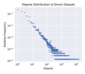
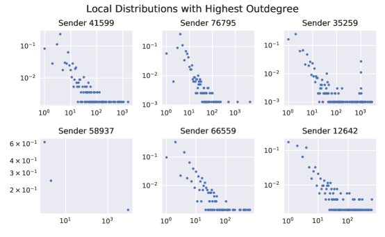
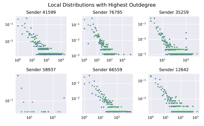
Figure 2 shows the global receiver degree distribution, as well as the local receiver distributions for the six senders with the largest number of emails. There is significant variation in behavior of the local degree distributions, both in comparison to themselves and to the behavior of the global degree distribution. This suggests that a modeling approach that allows for these differences is critical to accurately capturing the behavior of the entities, and thereby allowing for superior data summarization, sound inferences and strong prediction performance. While the Hollywood and GGP model would be unable to account for this variation, the proposed HVCM is equipped to capture this behavior.

7.2. Fit to the data

Figure 3. Trace plots and histograms for global parameters of the Enron data. Mixing occurs after 50 iterations or less. For the posterior predictive checks, the last 500 posterior samples were used.

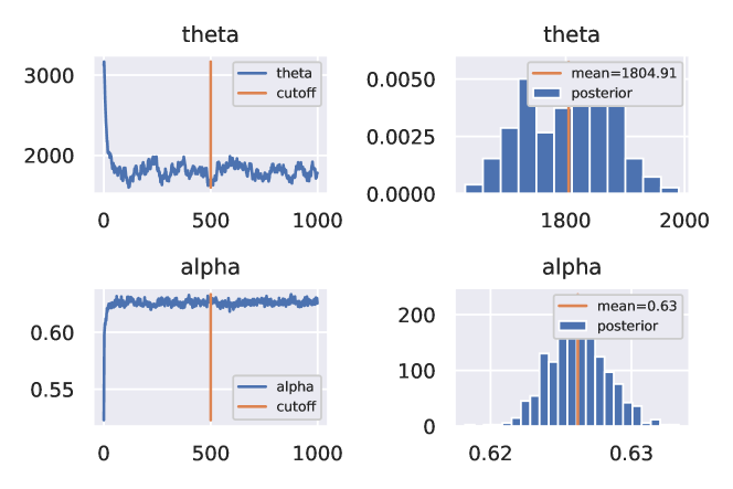
The Gibbs sampling algorithm introduced Section 6 is applied to the dataset for 1000 iterations, discarding the first 500 as burn-in. For this dataset, the following priors were used:

$$\mathop{\text{pr}}\nolimits(\theta)\sim\text{Gamma}(2,1000), \mathop{\text{pr}}\nolimits(\alpha)\sim\text{Beta}(1,1)$$

$$\mathop{\text{pr}}\nolimits(\theta_{s})\sim\text{Gamma}(1,20), \mathop{\text{pr}}\nolimits(\alpha_{s})\sim\text{Beta}(1,0.9)$$

Trace plots and histograms of the posterior samples of the global parameters $\alpha$ and $\theta$ are displayed in Figure 3. Note that discarding 500 posterior samples as burn-in is rather conservative, as the Gibbs sampler sampled chain mixes in less than 100 iterations.

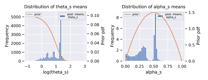
We show the histogram of posterior means of the local parameters $\theta_{s}$ and $\alpha_{s}$ in Figure 4, along with their priors. The $\theta_{s}$ parameters are shown on a log scale. These local histograms show significant diversity among the posterior parameter estimates, as we are fitting local variations in behavior. For $\alpha_{s}$, the choice of prior has very little effect on the posterior samples, except in the case of a small amount of local data for that particular sender $s$. The choice of prior for $\theta_{s}$ has more influence on the posterior distribution; our prior of $\text{Gamma}(1,20)$ is set to bias the local $\theta_{s}$ towards 0; this will allow for a better fit on the local data than a prior with larger variance or mean; this result is borne out when posterior predictive checks are applied to the local sender distributions, i.e., Figures 5 and 7.

Figure 4. Histograms of local $\alpha_{s}$ and $\theta_{s}$. Prior pdfs are shown in orange. The $\theta_{s}$ prior is set to fit the local distributions; the $\alpha_{s}$ posterior means are robust to the prior distribution chosen.

7.3. Posterior Predictive Checks (PPC) and Model Comparison

In this section, examples of posterior predictive model checks are shown in order to demonstrate the goodness of fit of the proposed HVCM. Posterior predictive checks are often used in order to verify that the proposed fitted model generates reasonable values on statistics of interest; these checks can also be used to diagnose where the model fails to perform well [45].

Multiple synthetic datasets are generated according to the posterior predictive distribution as prescribed in [45], and statistics of interest are calculated and compared with the statistics of the real data. The synthetic data is generated from the model with the parameters set to a posterior sample generated from the inference procedure. Since we are interested in the ability of the model to account for variation in local behavior, we take the sender sequence and number of receivers for each email as given, in order to directly compare the local receiver distributions of the posterior predictive data with the real data.

In addition to generating posterior predictive checks for the fitted HVCM, they are also generated for the Hollywood [7] and GGP [23] models for comparison. In the following subsections, a variety of posterior predictive statistics are described, both for the global dataset and for the local data per sender. These checks show that the proposed HVCM both provides a good global fit of the data, in addition to significantly improving the fit to local distributions compared to the Hollywood model. Table 1 details the 95% posterior predictive intervals for the global statistics, and Table 2 summarizes the posterior predictive coverage rate for local distributions for the proposed model and the Hollywood model. The statistics compared are number of unique receivers in the dataset and number of receivers with degree 1, 10, and 100.

7.3.1. Number of unique receivers

The first statistic we consider is the number of unique receivers, both in the global dataset as well as each local sender datasets. The number of unique receivers can be thought of as a surrogate for sparsity, and thus an important statistic for a candidate model to replicate. Figure 5 displays the results.

Figure 5. PPC Statistics for number of unique receivers, global (left) and examples of local (right).

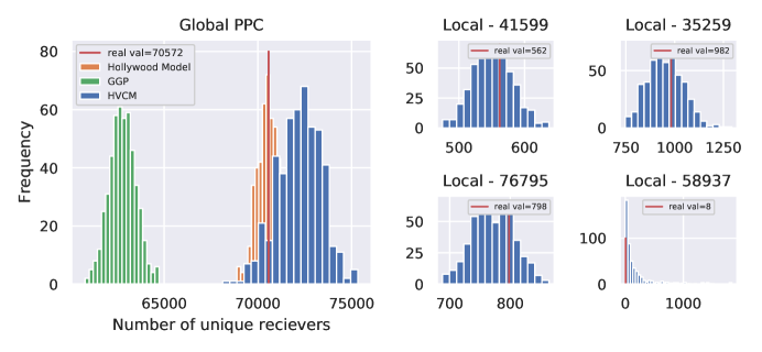
On the left plot, the PPC statistics are shown for the number of unique receivers in the global dataset. Both the Hollywood model and the proposed HVCM perform well on the global statistic. On the left plots are four examples of the PPC statistics for the number of unique receivers on the local sender datasets with the most emails. Only the results from the proposed HVCM is shown, because neither the GGP model nor the Hollywood model is able to take into account variation among the local distributions; if the sender labels are attached post-hoc to the synthetic data generated from the GGP or Hollywood model, they are completely unable to replicate any local behavior statistics. The HVCM clearly accounts for the varying local behavior, even when that local behavior is unusual (in the case of sender 58937). The superiority of the model compared to the Hollywood model is clearly shown in Table 2, as the proposed model’s local posterior predictive intervals in the local distributions covers the real values 99% of the time, as opposed to the Hollywood model’s coverage rate of 39%.

7.3.2. Degree distribution

Figure 6. Comparison of degree distribution between a posterior predictive sample from the proposed model and the real data (left) and PPC of the number of receivers with degree 10.

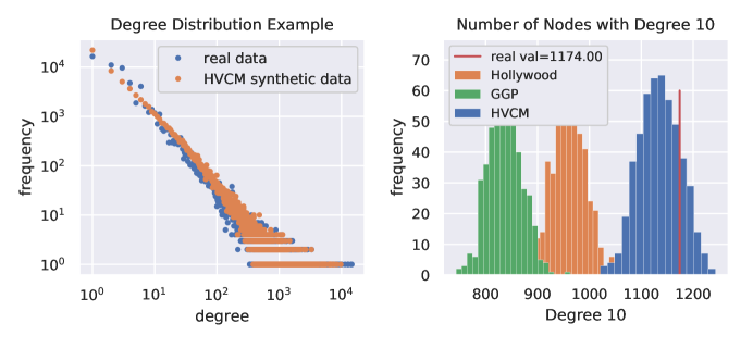
An important global behavior to capture is the global degree distribution. In order to evaluate this fit, posterior predictive intervals of the number of nodes with degree 1, 10, and 100 are shown in Table 1. Note that the HVCM performs the best, where the real number of receivers with degree 10 are within the PP interval. Figure 6 shows this result. When comparing the degree distributions, it is also clear that the Enron data does not perfectly align with the posterior predictive example, as the synthetic data overestimates the number of receivers with degree 1 and underestimates the number of receivers with degree 100. However, it is also clear that this model fit is still superior to both comparators, via Table 1. Further, Table 2 demonstrates that the coverage for the posterior predictive intervals is much more robust in the proposed model for each of the degree statistics. Figure 7 also compares local degree distributions between the HVCM and the real data. In the both the global and local case, the HVCM is able to better replicate the degree distribution.

Figure 7. Comparison of HVCM and Hollywood model for local distributions.

	Unique Receivers	Receivers with degree 1	Receivers with degree 10	Receivers with degree 100
HVCM	(69881, 74299)	(21504, 23022)	(1057, 1207)	(30, 56)
Hollywood Model	(69382, 71671)	(23031, 23997)	(893, 1022)	(31, 59)
GGP Model	(61309, 64175 )	(20653, 22006)	(778, 898)	(26, 51)
Actual Value	70572	16495	1174	15

Table 1. Posterior predictive confidence intervals (95%) for global statistics

	Unique Receivers	Receivers with degree 1	Receivers with degree 10	Receivers with degree 100
HVCM	19725 / 19752	18233 / 19752	808 / 960	14 / 22
Hollywood Model	7652 / 19752	7652 / 19752	48 / 960	1 / 22

Table 2. Posterior predictive coverage rates of the local distributions when using the 95% posterior predictive interval.

7.3.3. Node sharing across local distributions

In order to visualize how effectively the proposed HVCM is capturing the varying dependencies between the local and global distributions, we count the number of receivers that are seen in a particular number of local sender distributions. This allows for direct comparison of the effectiveness of the models to capture the interdependency and interaction among the local datasets. Figure 8 shows the results.

Figure 8. Distribution of nodes that have been in $x$ number of local sender distributions.

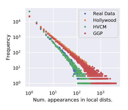
It is quite clear that the proposed HVCM replicates the observed behavior in the real data, while both the GGP and Hollywood models fail to capture the degree of pooling across the local datasets. Specifically, the other models seem to overestimate the rate at which receivers are shared across the local distributions.

7.3.4. L1 distance from degree distribution

Figure 9. Histograms of L1 distance between degree distributions of synthetic PPC datasets and Enron global degree distribution. The proposed model better captures the distribution than the Hollywood model and GGP model.

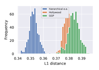
With our posterior predictive samples, we can also directly examine the difference in distribution between synthetic data and the real data. Figure 9 shows histograms of the TV distance between the global degree distributions of the synthetic data generated from the posterior predictive distribution and the real dataset. Again, the proposed HVCM leads to an improvement over the Hollywood model and GGP model.

8. ArXiv dataset

In this section, a larger and more complex dataset is used to demonstrate the flexibility of the proposed HVCM. The hierarchical exchangeable model is applied to the arXiv dataset https://archive.org/details/arxiv-bulk-metadata, which contains nearly all arXiv articles from 1986 to 2017. Like the Enron dataset, the arXiv data has a hierarchical structure — each article is required to have at least one associated subject. However, unlike the email dataset, which had only one sender per email, each article may have more than one subject. Our proposed model is well suited to this case of multiple entities and the data can still be appropriately represented by Equation 3. Further, our model allows for the direct study of interdisciplinarity among authors and overlap among the subject classes on arXiv.

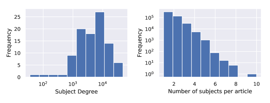
The arXiv subjects have been divided into 11 main classes; the full list can be found on https://arxiv.org/help/prep. In order to reduce the effect of author name ambiguity, we restricted ourselves to articles which have at least one subject from the math, cs, stat, and physics subject classes. A full description of the subjects of interest is found in section LABEL:appendix:arxiv of the supplementary materials. Figure 10 shows a degree distribution for the subjects, along with a histogram of the number of subjects per article. In total, there are 510812 scientific articles with 413029 unique authors and 130 unique subjects, There is also a broad range of subject frequencies, with the most popular subject being math-ph (mathematical physics) with 47942 articles, and the least popular subject cs.GL (general literature) with 130 articles.

Figure 10. Degree distribution of subjects, log scale. This degree distribution does not exhibit a power-law. The proposed HVCM accounts for this extra complexity. ($\alpha_{s}$ are not constrained to be equal to 1.)

We apply our posterior sampling methods found in Section 6, and in particular use the approximate method of calculating the posteriors of the indicator variables $Z_{i}$ using the methods described in Section 6.3. Trace plots of posterior estimates of certain parameters, posterior predictive checks for the data and other details of the inference can be found in section LABEL:appendix:arxiv of the supplementary materials.

8.1. Subject Overlap

The fitted model allows us to explore the amount of overlap between arXiv subjects. Two subjects are considered overlapping if the model has difficulty distinguishing between them when they are used as labels for the same article. This difficulty can be measured using the Shannon entropy, which is defined over discrete probability distributions $p=[p_{1},p_{2},\ldots,p_{k}]$ as:

$$H(p_{1},p_{2},\ldots,p_{k})=-\sum_{k}p_{k}\log_{2}p_{k}.$$

Entropy is at its maximum when the distribution $p$ is the uniform distribution, i.e., when all outcomes are equally likely. In order to estimate subject overlap for subjects $s_{1}$ and $s_{2}$, every article which lists $s_{1}$ and $s_{2}$ among its subjects is found, and the entropy of the posterior mean of the $Z_{i}$ distribution given that the subject is either $s_{1}$ or $s_{2}$ is calculated, and the entropy is averaged over the articles. This score, $\text{SO}(s_{1},s_{2})$ is computed as:

(21) $$\text{SO}(s_{1},s_{2})=\frac{1}{|\{\bar{S}_{i}:s_{1},s_{2}\in\bar{S}_{i}\}|}\sum_{i:s_{1},s_{2}\in\bar{S}_{i}}H(\mathop{\text{pr}}\nolimits(Z_{i}=s|\{\bar{S}_{i},\bar{R}_{i}\},Z_{i}\in\{s_{1},s_{2}\}))$$

Figure 11 shows a heatmap of the subject overlap scores for subjects that are seen in the same article at least 100 times. The subjects are ordered according to a normalized spectral clustering [46], using the subject overlap matrix SO as the affinity matrix, and setting the number of clusters to 6.

Figure 11. Heatmap of two-way entropy per article. For each pair of subjects $s_{1},s_{2}$, and every article that contains both $s_{1}$ and $s_{2}$, the entropy of $\mathop{\text{pr}}\nolimits(Z_{i}=z|Z_{i}\in\{s_{1},s_{2}\})$ is calculated and summed. Finally, each entry is normalized by the total number of occurences of $s_{1}$ and $s_{2}$ appearing together in the same article.

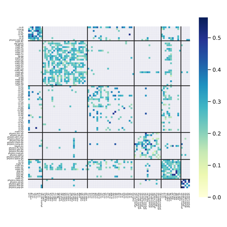
From this analysis, we conclude the following. Cluster 1, which includes cs.AI (Artificial Intelligence) and cs.IR (Information Retrieval), is a group of subjects that pertain to algorithmic approaches to artificial intelligence. Note that this cluster is differentiated from cluster 5, which tends to represent more theoretical papers that use statistics; this cluster includes math.ST (Statistical Theory), stat.ML (Machine Learning), and stat.ME (Methods). Cluster 2 can be considered the core math cluster, which encapsulates many pure and applied math subjects. Similarly, cluster 3 is the core computer science cluster, which are the computer science subjects that generally don’t use statistics such as cs.SE (Software Engineering) and cs.CE (Computer Engineering). Cluster 4 is the core physics cluster, with the subjects of physics that tend not to be interdisciplinary outside of physics as other physics subjects. Finally, cluster 6 consists of subjects that involve the philosophy, teaching or history of physics. Perhaps unsurprisingly, as AI is a fast moving field, two clusters are found (clusters 1 and 4) within AI that do not have a designated arXiv category. Table 3 lists the pairs of subjects with the most overlap according to the entropy score 21. Note that these pairs correspond with the general intuition of subjects that would have a large degree of interdisciplinarity.

Table 3. Pairs of subjects with highest subject overlap score.

$s_{1}$	$s_{2}$	$\text{SO}(s_{1},s_{2})$
stat.ME (Methods)	stat.CO (Computation)	0.509
cs.SE (Software Engineering)	cs.HC (High Perf. Comp.)	0.507
physics.class-ph (Classical Physics)	physics.ed-ph (Education)	0.504

We compare these results with results of a direct application of a spectral clustering algorithm to the co-authorship network in section LABEL:appendix:arxiv of the supplementary materials. This direct application of spectral clustering to the data is unable to recover the meaningful groupings that the proposed HVCM produces.

9. Concluding remarks

This paper has presented the class of exchangeable structured interaction models. By exploiting the common hierarchical nature of structured network data, complex models with both appropriate invariance and empirical properties are introduced. The canonical HVCM captures partial pooling of information, and can model complex local-behavior with global power-law degree behavior. A Gibbs sampling algorithm is proposed and applied to the Enron e-mail and arXiv datasets. The focus of this paper has been on e-mail and similarly structured interaction datasets. Extensions to more complex examples will be in considered future work. This paper lays the foundation for how the interaction exchangeability framework can account for complex behavior. Of course, many interaction networks occur with time-stamps; therefore, extensions to account for temporal dependence is required and will be an important next step .

References

- [1] A.-L. Barabási. Network Science. Cambridge University Press, 2016.
- [2] M. Newman. Networks: an introduction. Oxford University Press, 2010.
- [3] E. Estrada. The structure of complex networks: theory and applications. Oxford University Press, 2012.
- [4] V. Latora, V. Nicosia, and G. Russo. Complex networks: principles, methods and applications. Cambridge University Press, 2017.
- [5] Anna Goldenberg, Alice X. Zheng, Stephen E. Fienberg, and Edoardo M. Airoldi. A survey of statistical network models. Foundations and Trends in Machine Learning, 2(2):1–117, 2009.
- [6] Peter McCullagh. What is a statistical model? Ann. Statist., 30(5):1225–1310, 2002. With comments and a rejoinder by the author.
- [7] H. Crane and W. Dempsey. Edge exchangeable models for interaction networks. Journal of the American Statistical Association, 2017.
- [8] H. Crane and W. Dempsey. A framework for statistical network modeling. Statistical Science, 2018+.
- [9] S. Wasserman and P. Pattison. Logit models and logistic regressions for social networks: I. an introduction to markov graphs and p. Psychometrika, 61(3):401–425, 1996.
- [10] Edo M Airoldi, Thiago B Costa, and Stanley H Chan. Stochastic blockmodel approximation of a graphon: Theory and consistent estimation. In C. J. C. Burges, L. Bottou, M. Welling, Z. Ghahramani, and K. Q. Weinberger, editors, Advances in Neural Information Processing Systems 26, pages 692–700. Curran Associates, Inc., 2013.
- [11] P.W. Holland, K. Laskey, and S. Leinhardt. Stochastic blockmodels: First steps. Social Networks, 5(2):109–137, 1983.
- [12] J. R. Tyler, D.M. Wilkinson, and B.A. Huberman. E-mail as spectroscopy: Automated discovery of community structure within organizations. Inform. Soc., 21:143–153, 2005.
- [13] N. Eagle and A.S. Pentland. Reality mining: Sensing complex social systems. Pers. Ubiquit. Comput., 10:255–268, 2006.
- [14] J. H. Fowler. Connecting the congress: A study of cosponsorship networks. Polit. Anal., 14:456–487, 2006.
- [15] M. Signorelli and E.C. Wit. A penalized inference approach to stochastic block modelling of community structure in the italian parliament. Journal of the Royal Statistical Society: Series C, 67:355–369, 2018.
- [16] W. W. Cohen. Enron email dataset, August 2009.
- [17] Lorenzo A. Rossi and Omprakash Gnawali. Language Independent Analysis and Classification of Discussion Threads in Coursera MOOC Forums. In Proceedings of the IEEE International Conference on Information Reuse and Integration (IRI 2014), August 2014.
- [18] M. Luckie, Y. Hyun, and B. Huffaker. Traceroute probe method and forward ip path inference. In Proc. Internet Measurement Conference (IMC), pages 311–324, Oct. 2008.
- [19] Anna Goldenberg, Alice X Zheng, Stephen E Fienberg, Edoardo M Airoldi, et al. A survey of statistical network models. Foundations and Trends® in Machine Learning, 2(2):129–233, 2010.
- [20] P.O. Perry and P.J. Wolfe. Point process modelling for directed interaction networks. Journal of the Royal Statistical Society, Series B, 75:821–849, 2013.
- [21] D. R. Cox. Regression models and life-tables (with discussion). J. R. Statist. Soc. B, 34:187–220, 1972.
- [22] C.T. Butts. A relational event framework for social action. Sociol. Methodol., 38:155–200, 2008.
- [23] F. Caron and E.B. Fox. Bayesian nonparametric models of sparse and exchangeable random graphs. Journal of the Royal Statistical Society, Series B, 79(5):1295–1366, 2017.
- [24] Victor Veitch and Daniel M. Roy. The class of random graphs arising form exchangeable random. Accessed at arXiv:1512.03099, 2015.
- [25] V. Veitch and D. Roy. The class of random graphs arising from exchangeable random measures. arXiv:1512.03099 accessed at http://arxiv.org/pdf/1512.03099v1.pdf, 2015.
- [26] K. Bharath. Discussion of ”bayesian nonparametric models of sparse and exchangeable random graphs”. Journal of the Royal Statistical Society, Series B, 2017.
- [27] H. Crane. Discussion of ”bayesian nonparametric models of sparse and exchangeable random graphs”. Journal of the Royal Statistical Society, Series B, 2017.
- [28] E.M. Airoldi, D.S. Choi, and P.J. Wolfe. Confidence sets for network structure. Statistical Analysis and Data Mining, 4(5):461–469, 2011.
- [29] P. Latouche, S. Robin, and S. Ouadah. Goodness of fit of logistic models for random graphs. Available at arXiv:1508.00286, 2015.
- [30] M. Mariadassou, S. Robin, and C. Vacher. Uncovering latent structure in valued graphs: a variational approach. Annals of Applied Statistics, 4(2):715–742, 2010.
- [31] T.M. Sweet. Incorporating covariates into stochastic blockmodels. Journal of Educational and Behavioral Statistics, 40(6):634–664, 2015.
- [32] C. Tallberg. A bayesian approach to modeling stochastic block- structures with covariates. Journal of Mathematical Sociology, 29(1):1–23, 2004.
- [33] Y. Zhang, E. Levina, and J. Zhu. Community detection in networks with node features. Electronic journal of statistics, 10(2), 2016.
- [34] Harry Crane and Walter Dempsey. Relational exchangeability. arXiv preprint arXiv:1607.06762, 2016.
- [35] H. Crane and W. Dempsey. Edge exchangeable models for network data. arXiv:1603.04571, previously cited under original title Edge exchangeable network models and the power law, 2015, 2016.
- [36] J. Pitman. Combinatorial stochastic processes, volume 1875 of Lecture Notes in Mathematics. Springer-Verlag, Berlin, 2006.
- [37] H. Ishwaran and L. James. Gibbs sampling methods for stick-breaking priors. Journal of the American Statistical Association, 96(453):161–173, 2001.
- [38] David M Blei, Andrew Y Ng, and Michael I Jordan. Latent dirichlet allocation. Journal of machine Learning research, 3(Jan):993–1022, 2003.
- [39] Yee Whye Teh. A bayesian interpretation of interpolated kneserney. Technical report, National University of Singapore, 2006.
- [40] M. Escobar and M. West. Bayesian density estimation and inference using mixtures. Journal of the American Statistical Association, 90:577–588, 1995.
- [41] Bryan Klimt and Yiming Yang. The enron corpus: A new dataset for email classification research. In European Conference on Machine Learning, pages 217–226. Springer, 2004.
- [42] Andrew McCallum, Xuerui Wang, and Andrés Corrada-Emmanuel. Topic and role discovery in social networks with experiments on enron and academic email. Journal of Artificial Intelligence Research, 30:249–272, 2007.
- [43] Carey E Priebe, John M Conroy, David J Marchette, and Youngser Park. Scan statistics on enron graphs. Computational & Mathematical Organization Theory, 11(3):229–247, 2005.
- [44] Jorge Silva and Rebecca Willett. Hypergraph-based anomaly detection of high-dimensional co-occurrences. IEEE transactions on pattern analysis and machine intelligence, 31(3):563–569, 2009.
- [45] A. Gelman, X-L Meng, and H. Stern. Posterior predictive assessment of model fitness via realized discrepancies. Statistica Sinica, 6:733–807, 1996.
- [46] Andrew Y Ng, Michael I Jordan, and Yair Weiss. On spectral clustering: Analysis and an algorithm. In Advances in neural information processing systems, pages 849–856, 2002.