Lie Group Auto-Encoder

Abstract

In this paper, we propose an auto-encoder based generative neural network model whose encoder compresses the inputs into vectors in the tangent space of a special Lie group manifold: upper triangular positive definite affine transform matrices (UTDATs). UTDATs are representations of Gaussian distributions and can straightforwardly generate Gaussian distributed samples. Therefore, the encoder is trained together with a decoder (generator) which takes Gaussian distributed latent vectors as input. Compared with related generative models such as variational auto-encoder, the proposed model incorporates the information on geometric properties of Gaussian distributions. As a special case, we derive an exponential mapping layer for diagonal Gaussian UTDATs which eliminates matrix exponential operator compared with general exponential mapping in Lie group theory. Moreover, we derive an intrinsic loss for UTDAT Lie group which can be calculated as l-2 loss in the tangent space. Furthermore, inspired by the Lie group theory, we propose to use the Lie algebra vectors rather than the raw parameters (e.g. mean) of Gaussian distributions as compressed representations of original inputs. Experimental results verity the effectiveness of the proposed new generative model and the benefits gained from the Lie group structural information of UTDATs.

Figure 1: Overview of the proposed LGAE model. An input example $\vectorsym{x}$ is encoded into a vector in the tangent Lie algebra of the Lie group manifold formed by Gaussian distributions. Then, the vectors is mapped to a UTDAT representation of a Gaussian distribution. A latent vector is then sampled from this Gaussian distribution and fed to a decoder. The whole process is differentiable and optimized using stochastic gradient descent.

1 Introduction

Unsupervised deep learning is an active research area which shows considerable progresses recently. Many deep neural network models are invented to address various problems. For example, auto-encoders (AEs) (Hinton & Salakhutdinov, 2006) are used to learn efficient data codings, i.e. latent representations. Generative adversarial networks (GANs) (Goodfellow et al., 2014) are powerful on generating photo-realistic images from latent variables. While having achieved numerous successes, both AEs and GANs are not without their disadvantages. On one hand, AEs are good at obtaining a compressed latent representation of a given input, but hard to generate realistic samples randomly. On the other hand, GANs are good at randomly generating realistic samples, but hard to map a given input to its latent space representation. As a variant of AE, variational auto-encoders (VAEs) (Kingma & Welling, 2013) are another kind of generative models which can also obtain the latent representation of a given input. The architectures of VAEs are similar to AEs except that the encoders encode inputs into Gaussian distributions instead of deterministic vectors. Trained with a Bayesian framework, the decoder of a VAE is able to generate random samples from latent vectors which are Gaussian distributed random noises. As a result, many applications that require manipulating the latent space representations are also feasible with VAE.

One major problem of VAEs is that the geometric structure of Gaussian distributions is not considered. Traditional machine learning models including neural networks as the encoders of VAEs are designed for vector outputs. However, Gaussian distributions do not form a vector space. This can be easily shown because the parameter vectors are not closed under regular vector operators such as vector subtraction. The variance-covariance matrix must be positive definite but simple vector subtraction will break this requirement. Naively treating Gaussians as parameter vectors ignores the geometric structure information of the space formed by them. To exploit the geometric structural property, we need to identify what kind of space it is. Gong et al. (Gong et al., 2009) reveals that Gaussians can be represented as a special kind of affine transformations which are identified as a Lie group.

In this paper, we view Gaussian distributions from a geometrical perspective using Lie group theory, and propose a novel generative model using the encoder-decoder architecture. The overview of our model is presented in Figure 1. As illustrated therein, the central part of our model is a special Lie group: upper triangular positive definite affine transform matrices (UTDATs). On the one hand, UTDATs are matrix representations of Gaussian distributions. That’s to say, there is a one-to-one map between UTDATs and Gaussian distributions. Therefore, we can analyze the geometric properties of Gaussian distributions by analyzing the space of UTDAT. Also, we can sample from Gaussian distributions by matrix-vector multiplying UTDAT with a standard Gaussian noise vector. On the other hand, UTDATs form a Lie group. Therefore, one can work on the tangent spaces (which are Lie algebras) first, then project back to Lie group by exponential mapping. Since Lie algebras are vector spaces, they are suitable for most neural network architectures. As a result, the encoder in our model outputs vectors in the Lie algebra space. Those vectors are then projected to UTDATs by a proposed exponential mapping layer. Latent vectors are then generated by UTDATs and fed to a decoder. Specifically, for Gaussian distributions with diagonal variance-covariance matrices, we derive a closed form solution of exponential mapping which is fast and differentiable. Therefore, our model can be trained by stochastic gradient descents.

2 Related works

GANs (Goodfellow et al., 2014) (Zhang et al., 2018) (Miyato et al., 2018) (Mao et al., 2017) are proven effective in generating photo-realistic images in recent developments of neural networks. Because of the adversarial training approach, it is difficult for GANs to map inputs to latent vectors. Although some approaches (Donahue et al., 2016) (Schlegl et al., 2017) are proposed to address this problem, it still remains open and requires further investigation. Compared to GANs, VAEs (Kingma & Welling, 2013) (Doersch, 2016) are generative models which can easily map an input to its corresponding latent vector. This advantage enables VAEs to be either used as data compressors or employed in application scenarios where manipulation of the latent space is required (Yeh et al., 2016) (Deshpande et al., 2017). Compared with AEs (Hinton & Salakhutdinov, 2006), VAEs encode inputs to Gaussian distributions instead of deterministic latent vectors, and thus enable them to generate examples. On one hand, Gaussian distributions do not form a vector space. Naively treating them as vectors will ignore its geometric properties. On the other hand, most machine learning models including neural networks are designed to work with vector outputs. To incorporate the geometric properties of Gaussian distributions, the type of space of Gaussian distributions needs to be identified first; then corresponding techniques from geometric theories will be adopted to design the neural networks.

Geometric theories have been applied to analyze image feature space. In (Tuzel et al., 2008), covariance matrices are used as image feature representations for object detection. Because covariance matrices are symmetric positive definite (SPD) matrices, which form a Riemannian manifold, a corresponding boosting algorithm is designed for SPD inputs. In (Gong et al., 2009), Gaussian distributions are used to model image features and the input space is analyzed using Lie group theory.

In this paper, we propose a Lie group based generative model using the encoder-decoder architecture. The core of the model is Gaussian distributions, but we incorporate the geometric properties by working on the tangent space of Gaussian distributions rather than naively treating them as vectors.

3 Gaussians as Lie group

Let $\vectorsym{v}$ be a standard $n$-dimensional Gaussian random vector $\vectorsym{v}_{0}\sim{}\mathcal{N}(\vectorsym{0},\matrixsym{I})$, then any new vector $\vectorsym{v}=\matrixsym{A}\vectorsym{v}_{0}+\vectorsym{\mu}$ which is affine transformed from $\vectorsym{v}_{0}$ is also Gaussian distributed $\vectorsym{v}\sim{}\mathcal{N}(\vectorsym{\mu},\matrixsym{\Sigma})$, where $\matrixsym{\Sigma}=\matrixsym{A}\matrixsym{A}^{T}$. That is, any affine transformation can produce a Gaussian distributed random vector from the standard Gaussian. Furthermore, if we restrict the affine transformation to be $\vectorsym{v}=\matrixsym{U}\vectorsym{v}_{0}+\vectorsym{\mu}$ where $\matrixsym{U}$ is upper triangular and invertible (i.e. it has positive eigen values only), then conversely we can find a unique $U$ for any non-degenerate $\matrixsym{\Sigma}$ such that $\matrixsym{U}\matrixsym{U}^{T}=\matrixsym{\Sigma}$. In other words, non-degenerate Gaussian distributions are isomorphic to UTDATs. Let $G$ denote the matrix form of the following UTDAT:

$$\matrixsym{G}=\begin{bmatrix}\matrixsym{U}&\vectorsym{\mu}\\ 0&1\end{bmatrix},$$ (1)

then we can identify the type of spaces of Gaussian distributions by identifying the type of spaces of $G$.

According to Lie theory (Knapp, 2002), invertible affine transformations form a Lie group with matrix multiplication and inversion as its group operator. It can be easily verified that UTDATs are closed under matrix multiplication and inversion. So UTDATs form a subgroup of the general affine group. Since any subgroup of a Lie group is still a Lie group, UTDATs form a Lie group. In consequence, Gaussian distributions are elements of a Lie group.

A Lie group is also a differentiable manifold, with the property that the group operators are compatible with the smooth structure. An abstract Lie group has many isomorphic instances. Each of them is called a representation. In Lie theory, matrix representation is a useful tool for structure analysis. In our case, UTDAT is the matrix representation of the abstract Lie group formed by Gaussian distributions.

To exploit the geometric property of Lie group manifolds, the most important tools are logarithmic mapping, exponential mapping and geodesic distance. At a specific point of the group manifold, we can obtain a tangent space which is called Lie algebra in Lie theory. The Lie group manifold and Lie algebra are analogue to a curve and its tangent lines in a Euclidean space. Tangent spaces (i.e. Lie algebras) of a Lie group manifold are vector spaces. In our case, for $n$-dimensional Gaussians, the corresponding Lie group is $\frac{1}{2}n(n+3)$ dimensional. Accordingly, its tangent spaces are $\mathcal{R}^{\frac{1}{2}n(n+3)}$. Note that, at each point of the group manifold, we have a Lie algebra. We can project a point $\matrixsym{G}$ of the UTDAT group manifold to the tangent space at a specific point $\matrixsym{G}_{0}$ by the logarithmic mapping defined as

$$g=\log(\matrixsym{G}_{0}^{-1}\matrixsym{G}),$$ (2)

where the $\log$ operator at the right hand side is matrix logarithm operator. Note that the points are projected to a vector space even though the form of the results are still matrices, which means that we will flatten them to vectors wherever vectors are required. Specifically, the point $\matrixsym{G}_{0}$ will be projected to $\matrixsym{0}$ at its own tangent Lie algebra.

Conversely, the exponential mapping projects points in a tangent space back to the Lie group manifold. Let $\vectorsym{g}$ be a point in the tangent space of $\matrixsym{G}_{0}$, then the exponential mapping is defined as

$$G=\matrixsym{G}_{0}\exp(\vectorsym{g}),$$ (3)

where the $\exp$ operator at the right hand side is matrix exponential operator. For two points $\matrixsym{G}_{1}$ and $\matrixsym{G}_{2}$ of a Lie group manifold, the geodesic distance is the length of the shortest path connecting them along the manifold, which is defined as

$$d_{LG}(\matrixsym{G}_{1},\matrixsym{G}_{2})=\lVert\log(\matrixsym{G}_{1}^{-1}\matrixsym{G}_{2})\rVert_{F},$$ (4)

where $\lVert\cdot\rVert_{F}$ is the Frobenius norm.

4 Lie group auto-encoder

4.1 Overall architecture

Suppose we want to generate samples from a complex distribution $P(\vectorsym{X})$ where $\vectorsym{X}\in\mathcal{R}^{D}$. One way to accomplish this task is to generate samples from a joint distribution $P(\vectorsym{Z},\vectorsym{X})$ first, then discard the part belonging to $\vectorsym{Z}$ and keep the part belonging to $\vectorsym{X}$ only. This seems giving us no benefit at first sight because it is usually difficult to sample from $P(\vectorsym{Z},\vectorsym{X})$ if sampling from $P(\vectorsym{X})$ is hard. However, if we decompose the joint distribution with a Bayesian formula

$$P(\vectorsym{Z},\vectorsym{X})=P(\vectorsym{X}|\vectorsym{Z})P(\vectorsym{Z}),$$ (5)

then the joint distribution can be sampled by a two step process: Firstly sample from $P(\vectorsym{Z})$, then sample from $P(\vectorsym{X}|\vectorsym{Z})$. The benefits come from the fact that both $P(\vectorsym{Z})$ and $P(\vectorsym{X|Z})$ may be much easier to sample from.

Estimating parameters in $P(\vectorsym{Z},\vectorsym{X})$ as modeled in Eq. 5 is not easy because samples from the joint distribution are required; however, in most scenarios, we only have samples $\{\vectorsym{x}_{i}:i=1,2,\cdots,n\}$ from the marginal distribution $P(\vectorsym{X})$. To overcome this problem, we augment each example $\vectorsym{x}_{i}$ from the marginal distribution to several examples $\{(\vectorsym{z}_{ij},\vectorsym{x}_{i}):j=1,2,\cdots,m\}$ in the joint distribution by sampling $\vectorsym{z}_{ij}$ from the conditional distribution $P(\vectorsym{Z}|\vectorsym{X})$.

Note that $Z$ is an auxiliary random vector helping us perform sampling from the marginal distribution $P(\vectorsym{X})$, so it can be any kind of distribution but should be easy to sample from. In this paper, we let $P(\vectorsym{Z})\sim\mathcal{N}(\vectorsym{0},\matrixsym{I})$.

In practice, $P(\vectorsym{Z}|\vectorsym{X})$ should be chosen according to the type of data space of $\vectorsym{X}$. For example, if $X$ is continuous, we can model $P(\vectorsym{X}|\vectorsym{Z})$ as a Gaussian distribution with a fixed isotropic variance-covariance matrix. For binary and categorical typed $\vectorsym{X}$, Bernoulli and multinomial distributions can be used, respectively.

Given $P(\vectorsym{Z})$ and $P(\vectorsym{X}|\vectorsym{Z})$, $P(\vectorsym{Z}|\vectorsym{X})$ is usually complex and thus difficult to sample from. So we sample $\vectorsym{z}_{ij}$ from another distribution $Q(\vectorsym{Z}|\vectorsym{X})$ instead. In this paper, we model $Q(\vectorsym{Z}|\vectorsym{X})$ as Gaussian distributions with diagonal variance-covariance matrices. $Q(\vectorsym{Z}|\vectorsym{X})$ should satisfy the following objectives as much as possible:

• $Q(\vectorsym{Z}|\vectorsym{X})$ should approximate $P(\vectorsym{Z}|\vectorsym{X})$. Therefore, given $\vectorsym{z}_{ij}$ sampled from $Q(\vectorsym{Z}|\vectorsym{x}_{i})$, $\hat{\vectorsym{x}}_{i}$ sampled from $P(\vectorsym{X}|\vectorsym{Z})$ should reconstruct $\vectorsym{x}_{i}$.

• $\{\vectorsym{z}_{ij}:i=1,2,\cdots,n;j=1,2,\cdots,m\}$ should fit the marginal $P(\vectorsym{Z})$ well.

To optimize the first objective, we minimize the reconstruction loss $L_{rec}$, which is the mean squared error (MSE) for continuous $\vectorsym{X}$ and cross-entropy for binary and categorical $\vectorsym{X}$.

For the second objective, directly optimizing it using $\vectorsym{z}_{ij}$ is not practical because we need a large sample size $m$ for $P(\matrixsym{Z}|\matrixsym{X})$ to accurately estimate model parameters. The total sample size of $\vectorsym{z}_{ij}$, which is $mn$, is too big for computation. To overcome this problem, we consider Gaussian distributions as points in the corresponding Lie group as we discussed in section 3. Note that the set $\{\vectorsym{z}_{ij},i=1,2,\cdots,n;j=1,2,\cdots,m\}$ is sampled from a set of Gaussian distributions $Q(\vectorsym{Z}|\vectorsym{x}_{i})$. The second objective implies the average distribution of those Gaussians should be $P(\vectorsym{Z})$, which is a standard Gaussian. However, Gaussian distributions, which are equivalently represented as UTDATs, do not conform to the commonly used Euclidean geometry. Instead, we need to find the intrinsic mean of those Gaussians through Lie group geometry because Gaussian distributions have a Lie group structure. We derive a Lie group intrinsic loss $L_{LG}$ to optimize the second objective. The details of $L_{LG}$ will be present in subsection 4.3.

In our proposed Lie group auto-encoder (LGAE), $P(\vectorsym{X}|\vectorsym{Z})$ is called a decoder or generator, and is implemented with neural networks. $Q(\vectorsym{Z}|\vectorsym{X})$ is also implemented with neural networks. Note that $Q(\vectorsym{Z}|\vectorsym{X})$ is a Gaussian distribution, so the corresponding neural network is a function whose output is a Gaussian distribution. Neural networks as well as many other machine learning models are typically designed for vector outputs. Being intrinsically a Lie group as discussed in section 3, Gaussian distributions do not form a vector space. To best exploit the geometric structure of the Gaussians, we first estimate corresponding points $\matrixsym{g}_{i}$ in the tangent Lie algebra at the position of the intrinsic mean of $\{\matrixsym{G}_{i},i=1,2,\cdots,n\}$ using neural networks. As $L_{LG}$ requires the intrinsic mean to be the standard Gaussian $P(\vectorsym{Z})=\mathcal{N}(\vectorsym{0},\matrixsym{I})$, whose UTDAT representation is the identity matrix $\matrixsym{I}$, the corresponding point $\matrixsym{g}_{i}$ in the tangent space of $\matrixsym{G}_{i}$ is

$$\matrixsym{g}_{i}=\log(\matrixsym{G}_{i}).$$ (6)

Since $\{\matrixsym{g}_{i},i=1,2,\cdots,n\}$ are in a vector space, they can be well estimated by neural networks. $\matrixsym{g}_{i}$s are then projected to the Lie group by an exponential mapping layer

$$\matrixsym{G}_{i}=\exp(\matrixsym{g}_{i}).$$ (7)

For diagonal Gaussians, we derive a closed-form solution of the exponential mapping which eliminates the requirement of matrix exponential operator. The details will be presented in subsection 4.2.

The whole architecture of LGAE is summarized in Figure 1. A typical forward procedure works as follows: Firstly, the encoder encodes an input $\vectorsym{x}_{i}$ into a point $\matrixsym{g}_{i}$ in the tangent Lie algebra. The exponential mapping layer then projects $\matrixsym{g}_{i}$ to the UTDAT matrix $\matrixsym{G}_{i}$ of the Lie group manifold. A latent vector $\vectorsym{z}$ is then sampled from the Gaussian distribution represented by $\matrixsym{G}_{i}$ by multiplying $\matrixsym{G}_{i}$ with a standard Gaussian noise vector. The details of the sampling operation will be described in section 4.4. The decoder (or generator) network then generates $\hat{\vectorsym{x}}_{i}$ which is the reconstructed version of $\vectorsym{x}_{i}$. The whole network is optimized by minimizing the following loss

$$L=\lambda{}L_{LG}+L_{rec},$$ (8)

where $L_{LG}$ and $L_{rec}$ are the Lie group intrinsic loss and reconstruction loss, respectively. Because the whole forward process and the loss are differentiable, the optimization can be achieved by stochastic gradient descent method.

4.2 Exponential mapping layer

We derive the exponential mapping $\matrixsym{g}_{i}=\exp({\matrixsym{G}_{i}})$ for diagonal Gaussians. When $\matrixsym{G}_{i}\sim\mathcal{N}(\vectorsym{\mu}_{i},\matrixsym{\Sigma}_{i})$ is diagonal, we have

$$\matrixsym{\Sigma}_{i}=\begin{bmatrix}\sigma_{i1}^{2}&&\\ &\sigma_{i2}^{2}&\\ &&\ddots&\\ &&&\sigma_{iK}^{2}.\end{bmatrix}.$$ (9)

The following theorem gives the forms of $\matrixsym{G}_{i}$ and $\matrixsym{g}_{i}$, as well as their relationship.

Theorem 1.

Let $\matrixsym{G}_{i}$ be the UTDAT and $\matrixsym{g}_{i}$ be the corresponding vector in its tangent Lie algebra at the standard Gaussian. Then

$$\matrixsym{G}_{i} =\begin{bmatrix}\sigma_{i1}&&&\mu_{i1}\\ &\sigma_{i2}&&\mu_{i2}\\ &&\ddots&\vdots\\ 0&0&\ldots&1\end{bmatrix}$$ (10)

$$\matrixsym{g}_{i} =\begin{bmatrix}\phi_{i1}&&&\theta_{i1}\\ &\phi_{i2}&&\theta_{i2}\\ &&\ddots&\vdots\\ 0&0&\ldots&1\end{bmatrix},$$ (11)

where

$$\phi_{ik} =\log(\sigma_{ik})$$ (12)

$$\theta_{ik} =\frac{\mu_{ik}\log(\sigma_{ik})}{\sigma_{ik}-1}.$$ (13)

Proof.

By the definition of UTDAT, we can straightforwardly get Eq. 10. Let $\matrixsym{H}=\matrixsym{G}_{i}-\matrixsym{I}$. Using the series form of matrix logarithm, we have

$$\matrixsym{g}_{i} =\log(\matrixsym{G}_{i})$$

$$=\log(\matrixsym{I}+\matrixsym{H})$$

$$=\sum_{t=1}^{\infty}(-1)^{t-1}\frac{\matrixsym{H}^{t}}{t}.$$ (14)

By substituting $\matrixsym{H}$ into 14, we get Eq. 11 and the following:

$$\phi_{ik} =\sum\limits_{t=1}^{\infty}(-1)^{t-1}\frac{(\sigma_{ik}-1)^{t}}{t}$$

$$=\log(\sigma_{ik})$$

and

$$\theta_{ik} =\sum\limits_{t=1}^{\infty}(-1)^{t-1}\frac{\mu_{ik}(\sigma_{ik}-1)^{t-1}}{t}$$

$$=\frac{\mu_{ik}\log(\sigma_{ik})}{\sigma_{ik}-1}.$$

Alternatively, after we identify $\matrixsym{g}_{i}$ has the form as in Eq. 11, we can derive the exponential mapping by the definition of matrix exponential

$$\matrixsym{G}_{i} =\exp(\matrixsym{g}_{i})=\sum_{t=0}^{\infty}\frac{\matrixsym{g}_{i}^{t}}{t!}$$

$$=\begin{bmatrix}\sum_{t=0}^{\infty}\frac{\phi_{i1}^{t}}{t!}&&\theta_{i1}\sum_{t=1}^{\infty}\frac{\phi_{i1}^{t-1}}{t!}\\ &\ddots&\vdots\\ 0&\ldots&1\end{bmatrix}$$

$$=\begin{bmatrix}e^{\phi_{i1}}&&\frac{\theta_{i1}}{\phi_{i1}}\left(\sum_{t=0}^{\infty}\frac{\phi_{i1}^{t}}{t!}-1\right)\\ &\ddots&\vdots\\ 0&\ldots&1\end{bmatrix}$$

$$=\begin{bmatrix}e^{\phi_{i1}}&&\frac{\theta_{ik}(e^{\phi_{i1}}-1)}{\phi_{i1}}\\ &\ddots&\vdots\\ 0&\ldots&1\end{bmatrix}.$$

∎

The exponential mapping layer is expressed as

$$\sigma_{ik} =e^{\phi_{ik}}$$ (15)

$$\mu_{ik} =\frac{\theta_{ik}(e^{\phi_{ik}}-1)}{\phi_{ik}}$$ (16)

Note that if $\sigma_{ik}=1$ (i.e. $\phi_{ik}=0$), then $\mu_{ik}=\theta_{ik}$ due to the fact that $\lim_{x\to{}0}\frac{\log(x+1)}{x}=1$ or $\lim_{x\to{}0}\frac{e^{x}-1}{x}=1$.

4.3 Lie group intrinsic loss

Let $\matrixsym{G}_{i}$ be the UTDAT representation of $P(\vectorsym{Z}|\vectorsym{x}_{i})$. The intrinsic mean $\matrixsym{G}^{*}$ of those $\matrixsym{G}_{i}$s is defined as

$$\matrixsym{G}^{*}=\underset{\matrixsym{G}}{\arg\min}\sum_{i=1}^{n}d_{LG}^{2}(\matrixsym{G},\matrixsym{G}_{i}).$$ (17)

The second objective in the previous subsection requires that $\matrixsym{G}^{*}=\matrixsym{I}$, which is equivalent to minimizing the loss

$$L_{LG} =\sum_{i=1}^{n}d_{LG}^{2}(\matrixsym{I},\matrixsym{G}_{i})$$ (18)

$$=\sum_{i=1}^{n}\lVert\log(\matrixsym{G}_{i})\rVert_{F}^{2}$$

$$=\sum_{i=1}^{n}\lVert\matrixsym{g}_{i}\rVert_{F}^{2}.$$ (19)

So the intrinsic loss plays a role of regularization during the training. Since the tangent Lie algebra is a vector space, the Frobenius norm is equivalent to the $l^{2}$-norm if we flatten matrix $\matrixsym{g}_{i}$ to a vector. Eq. 18 plays a role of regularization which requires all the Gaussians $\matrixsym{G}_{i}$ to be grouped together around the standard Gaussian. Eq. 19 shows that we can regularize on the tangent Lie algebra instead, which avoids the matrix logarithm operation. Specifically, for diagonal Gaussians, we have

$$L_{LG} =\sum_{i=1}^{n}\lVert\matrixsym{g}_{i}\rVert_{F}^{2}$$ (20)

$$=\sum_{i=1}^{n}\sum_{k=1}^{K}(\phi_{ik}^{2}+\theta_{ik}^{2})$$ (21)

4.4 Sampling from Gaussians

According to the properties of Gaussian distributions discussed in section 3, sampling from an arbitrary Gaussian distribution can be achieved by transforming a standard Gaussian distribution with the corresponding, i.e.

$$\begin{bmatrix}\vectorsym{z}_{ij}\\ 1\end{bmatrix}=\matrixsym{G}_{i}\begin{bmatrix}\vectorsym{v}_{ij}\\ 1\end{bmatrix},$$ (22)

where $\vectorsym{v}_{ij}$ is sample from $\vectorsym{V}\sim\mathcal{N}(\vectorsym{0},\matrixsym{I})$. Note that, this sampling operator is differentiable, which means that gradients can be back-propagated through the sampling layer to the previous layers. When $\matrixsym{G}_{i}$ is a diagonal Gaussian, we have

$$\vectorsym{z}_{ij}=\vectorsym{\sigma}\odot\vectorsym{v}_{ij}+\vectorsym{\mu},$$ (23)

where $\vectorsym{\sigma}=[\sigma_{i1},\cdots,\sigma_{iK}]^{T}$, $\vectorsym{\mu}=[\mu_{i1},\cdots,\mu_{iK}]^{T}$ and $\odot$ is the element-wise multiplication. Therefore, the re-parameterization trick in (Kingma & Welling, 2013) is a special case of sampling of UTDAT represented Gaussian distributions.

MNIST (K=2)	MNIST (K=5)	MNIST (K=10)	MNIST (K=20)
	SVHN (K=2)	SVHN (K=5)	SVHN (K=10)

Figure 2: Loss values (i.e. negative lower bound of marginal likelihood as described in (Kingma & Welling, 2013)) versus training progresses. The horizontal and vertical axes are the number of epochs trained and the loss values, respectively. Note that loss values on the SVHN dataset are plotted with two different vertical axes to avoid the scaling problem caused by the gap between training and testing loss values. The left and right axes are for traing and testing sets, respectively.

5 Discussion

Although our proposed LGAE and VAE both (Kingma & Welling, 2013) have an encoder-decoder based architecture, they are essentially different. The loss function of VAE, which is

$$L=\operatorname{KL}(Q(\vectorsym{Z}|\vectorsym{X})\rVert\mathcal{N}(\vectorsym{0},\matrixsym{I}))+L_{rec},$$ (24)

is derived from the Bayesian lower bound of the marginal likelihood of the data. In contrast, the loss function of LGAE is derived from a geometrical perspective. Further, the Lie group intrinsic loss $L_{LG}$ in Eq. (8) is a real metric, but the KL-divergence in Eq. (24) is not. For examples, the KL-divergence is not symmetric, nor does it satisfy the triangle inequality.

Further, while both LGAE and VAE estimate Gaussian distributions using neural networks, VAE does not address the non-vector output problem. As a contrast, we systematically address this problem and design an exponential mapping layer to solve it. One requirement arising from the non-vector property of Gaussian distributions is that the variance parameters be positive. To satisfy this requirement, (Kingma & Welling, 2013) estimate the logarithm of variance instead. This technique is equivalent to performing the exponential mapping for the variance part. Without a theoretical foundation, it was trial-and-error to choose exp over other activations such as relu and softplus. Our theoretical results confirms that exp makes more sense than others. Moreover, our theoretical results further show that a better way is to consider a Gaussian distribution as a whole rather than treat its variance part only and address the problem in an empirical way.

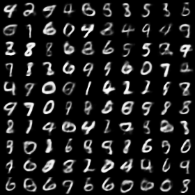
Because the points of the tangent Lie algebra are already vectors, we propose to use them as compressed representations of the input data examples. These vectors contain information of the Gaussian distributions and already incorporate the Lie group structural information of the Gaussian distributions; therefore, they are more informative than either a single mean vector or concatenating the mean vector and variance vector naively together.

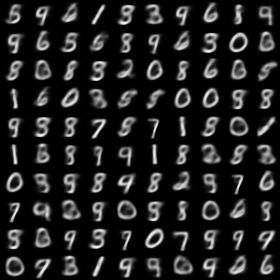
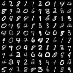
VAE (K=2)	VAE (K=5)	VAE (K=10)	VAE (K=20)
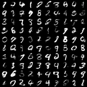
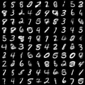
LGAE (K=2)	LGAE (K=5)	LGAE (K=10)	LGAE (K=20)

Figure 3: Generated images from randomly sampled latent vectors for the MNIST dataset. The upper and lower rows are generated by the VAE and LGAE models, respectively.

6 Experiments

6.1 Datasets

The proposed LGAE model is evaluated on two benchmark datasets:

• MNIST: The MNIST dataset (Lecun et al., 1998) consists of a training set of $60,000$ examples of handwritten digits, and a test set of $10,000$ examples. The digits have been size-normalized and centered into fixed-size $28\times{}28$ images.

• SVHN: The SVHN dataset (Netzer et al., 2011) is also a collection of images of digits. But the background of image is more clutter than MNIST, so it is significantly harder to classify. It includes a training set of $73,257$ examples, a test set of $26,032$ examples, and an extra training set of $531,131$ examples. In our experiments, we use the training and test sets only, and the extra training set is not used throughout the experiments.

6.2 Settings

Since VAE (Kingma & Welling, 2013) is the most related model of LGAE, we use VAE as a baseline for comparisons. We follow the exact experimental settings of (Kingma & Welling, 2013). That is, MLP with $500$ hidden units are used as encoder and decoder. In each hidden layer, non-linear activation tanh are applied. The parameters of neurons are initialized by random sampling from $\mathcal{N}(0,0.01)$ and are optimized by Adagrad (Duchi et al., 2011) with learning rate $0.01$. Mini-batches of size $100$ are used. For the LGAE model, we use $\lambda=0.5$ as the weight for the Lie group intrinsic loss.

For both the MNIST and SVHN datasets, we normalize the pixel values of the images to be in the range $[0,1]$. Cross entropies between those true pixel values and predicted values are used as reconstruction errors in Eq. (8). Both the VAE and LGAE are implemented with PyTorch (Paszke et al., 2017). Note that there is no matrix operation in the LGAE implementation thanks to the element-wise closed-form solution presented in Section 4.2 and 4.3. Therefore, the run-time is almost the same as VAE. On a Nvidia GeForce GTX 1080 graphic card, it takes about $12.5$ and $25$ seconds to train on the training set and test on both the training and test sets for one epoch with mini-batches of size $100$.

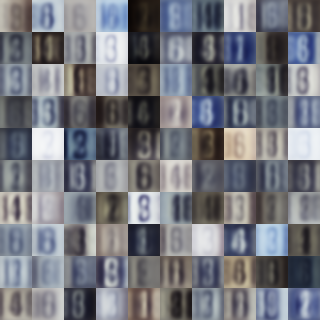VAE (K=2)	VAE (K=5)	VAE (K=10)
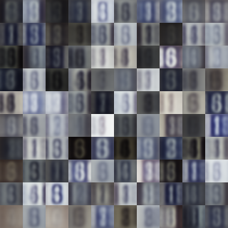
LGAE (K=2)	LGAE (K=5)	LGAE (K=10)

Figure 4: Generated images from randomly sampled latent vectors for the MNIST dataset. The upper and lower rows are generated by the VAE and LGAE models, respectively.

6.3 Results

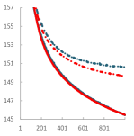
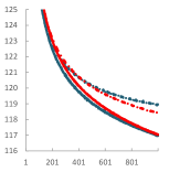
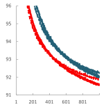
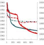
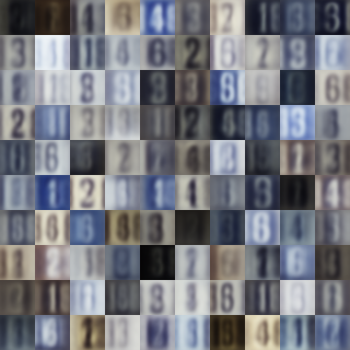
In the first experiment, we investigate the effectiveness of the proposed exponential mapping layer. We design a variant of LGAE which uses the same loss as VAE; i.e., we replace the Lie group intrinsic loss with KL divergence but keep the exponential mapping layer in the model. We call this variant LGAE-KL. Because it has the same loss formula as VAE, it is fair to compare their values during training. We train VAE and LGAE-KL on the training sets of MNIST and SVHN for $1,000$ epochs. It is shown in (Kingma & Welling, 2013) that the negative value of this loss is the lower bound of the marginal likelihood in a Bayesian perspective. After each epoch, we evaluate the loss both on the training and test sets. The values are plotted in Figure 2. The curves show that our LGAE-KL obtains smaller values of the loss both on training and test sets, which indicates that learning on the tangent Lie algebra is more effective than ignoring the Lie group structure of the Gaussian distributions. Note that LGAE also obtains smaller lower bounds consistently with different values of $K$. On the SVHN dataset, there is a large gap between training and testing loss values, which is possibly caused by the different sizes of the two sets, as well as the cluttered backgrounds in images of the dataset. A simple multi-layer perceptrons (MLP) network with two layers may not be able to sufficiently fit the data; therefore, the lower bound value on the training set decreases too slowly to close the gap. In the future, designing a deep convolutional network architecture for the encoder and decoder is a promising direction to extend LGAE model to handle natural images.

In the second experiment, we compare the encoding capability of LGAE with VAE. We train LGAE, LGAE-KL and VAE on the training sets. Then we obtain the encoded representations of examples from both the training and test sets. A nearest centroid classifier is then trained on the representations of the training set and tested on the test set. Since the nearest centroid is a very simple classifier which has no hyper-parameters, the classification accuracy on the test set indicates the representation power of encoded inputs. For VAE we test two different representations: mean vector and a concatenation of mean vector and covariance matrix (i.e. concatenate parameters of Gaussian distributions). For LGAE-KL and LGAE we test those two kinds of representations as well as the Lie algebra vector. Table 1 summarizes the results on the MNIST dataset.

Table 1: Classification accuracies ($\%$) on the MNIST dataset.

Method	$K=2$	$K=5$	$K=10$
VAE ($\vectorsym{\mu}$)	$56.22$	$78.53$	$85.68$
VAE ($\vectorsym{\mu}\|\matrixsym{\Sigma}$)	$56.22$	$78.53$	$85.68$
LGAE-KL ($\vectorsym{\mu}$)	$58.88$	$80.77$	$85.86$
LGAE-KL ($\vectorsym{\mu}\|\matrixsym{\Sigma}$)	$58.88$	$80.77$	$85.90$
LGAE-KL ($\matrixsym{g}$)	$60.82$	$80.54$	$86.20$
LGAE ($\vectorsym{\mu}$)	$59.37$	$79.81$	$85.45$
LGAE ($\vectorsym{\mu}\|\matrixsym{\Sigma}$)	$54.80$	$79.26$	$85.47$
LGAE ($\matrixsym{g}$)	$\bm{68.70}$	$\bm{83.27}$	$\bm{86.88}$

From Table 1, we can see that LGAE-KL gets better performance than VAE, which reconfirms the effectiveness of the proposed exponential mapping layer. LGAE performs the best, which indicates the superiority of the Lie group intrinsic loss over KL divergence. Moreover, the results also show that naively concatenating covariance with mean does not contribute much to the performances, and sometimes even hurts it. This phenomenon indicates that treating Gaussians as vectors cannot fully extract important geometric structural information from the manifold they formed.

To illustrate the generative capability of LGAE, we randomly generate images using the model and plot them along with images generated from VAE. Figures 3 and 4 show the generated images from both models trained on the MNIST and SVHN datasets, respectively.

7 Conclusions

We propose Lie group auto-encoder (LGAE), which is a encoder-decoder type of neural network model. Similar to VAE, the proposed LGAE model has the advantages of generating examples from the training data distribution, as well as mapping inputs to latent representations. The Lie group structure of Gaussian distributions is systematically exploited to help design the network. Specifically, we design an exponential mapping layer, derive a Lie group intrinsic loss, and propose to use Lie algebra vectors as latent representations. Experimental results on the MNIST and SVHN datasets testify to the effectiveness of the proposed method.

References

- Deshpande et al. (2017) Deshpande, A., Lu, J., Yeh, M., Chong, M. J., and Forsyth, D. Learning Diverse Image Colorization. In 2017 IEEE Conference on Computer Vision and Pattern Recognition (CVPR), pp. 2877–2885, July 2017.
- Doersch (2016) Doersch, C. Tutorial on Variational Autoencoders. arXiv:1606.05908 [cs, stat], June 2016.
- Donahue et al. (2016) Donahue, J., Krähenbühl, P., and Darrell, T. Adversarial Feature Learning. arXiv:1605.09782 [cs, stat], May 2016.
- Duchi et al. (2011) Duchi, J., Hazan, E., and Singer, Y. Adaptive Subgradient Methods for Online Learning and Stochastic Optimization. Journal of Machine Learning Research, 12(Jul):2121–2159, 2011.
- Gong et al. (2009) Gong, L., Wang, T., and Liu, F. Shape of Gaussians as feature descriptors. In IEEE Conference on Computer Vision and Pattern Recognition, pp. 2366–2371, June 2009.
- Goodfellow et al. (2014) Goodfellow, I., Pouget-Abadie, J., Mirza, M., Xu, B., Warde-Farley, D., Ozair, S., Courville, A., and Bengio, Y. Generative Adversarial Nets. In Advances in Neural Information Processing Systems, pp. 9, 2014.
- Hinton & Salakhutdinov (2006) Hinton, G. E. and Salakhutdinov, R. R. Reducing the Dimensionality of Data with Neural Networks. Science, 313(5786):504–507, July 2006.
- Kingma & Welling (2013) Kingma, D. P. and Welling, M. Auto-Encoding Variational Bayes. arXiv:1312.6114 [cs, stat], December 2013.
- Knapp (2002) Knapp, A. W. Lie Groups Beyond an Introduction. Progress in Mathematics. Birkhäuser Basel, 2 edition, 2002. ISBN 978-0-8176-4259-4.
- Lecun et al. (1998) Lecun, Y., Bottou, L., Bengio, Y., and Haffner, P. Gradient-based learning applied to document recognition. Proceedings of the IEEE, 86(11):2278–2324, November 1998.
- Mao et al. (2017) Mao, X., Li, Q., Xie, H., Lau, R. Y. K., Wang, Z., and Smolley, S. P. Least Squares Generative Adversarial Networks. In International Conference on Computer Vision, pp. 9, 2017.
- Miyato et al. (2018) Miyato, T., Kataoka, T., Koyama, M., and Yoshida, Y. Spectral Normalization for Generative Adversarial Networks. In International Conference on Learning Representations, February 2018.
- Netzer et al. (2011) Netzer, Y., Wang, T., Coates, A., Bissacco, A., Wu, B., and Ng, A. Y. Reading Digits in Natural Images with Unsupervised Feature Learning. In NIPS Workshop on Deep Learning and Unsupervised Feature Learning, pp. 9, 2011.
- Paszke et al. (2017) Paszke, A., Gross, S., Chintala, S., Chanan, G., Yang, E., DeVito, Z., Lin, Z., Desmaison, A., Antiga, L., and Lerer, A. Automatic differentiation in PyTorch. In NIPS Workshop Autodiff, October 2017.
- Schlegl et al. (2017) Schlegl, T., Seeböck, P., Waldstein, S. M., Schmidt-Erfurth, U., and Langs, G. Unsupervised Anomaly Detection with Generative Adversarial Networks to Guide Marker Discovery. In Niethammer, M., Styner, M., Aylward, S., Zhu, H., Oguz, I., Yap, P.-T., and Shen, D. (eds.), Information Processing in Medical Imaging, Lecture Notes in Computer Science, pp. 146–157. Springer International Publishing, 2017. ISBN 978-3-319-59050-9.
- Tuzel et al. (2008) Tuzel, O., Porikli, F., and Meer, P. Pedestrian Detection via Classification on Riemannian Manifolds. IEEE Transactions on Pattern Analysis and Machine Intelligence, 30(10):1713–1727, October 2008.
- Yeh et al. (2016) Yeh, R., Liu, Z., Goldman, D. B., and Agarwala, A. Semantic Facial Expression Editing using Autoencoded Flow. arXiv:1611.09961 [cs], November 2016.
- Zhang et al. (2018) Zhang, H., Goodfellow, I., Metaxas, D., and Odena, A. Self-Attention Generative Adversarial Networks. arXiv:1805.08318 [cs, stat], May 2018.